WARM: A Weakly (+Semi) Supervised Math Word Problem Solver

Abstract

Solving math word problems (MWPs) is an important and challenging problem in natural language processing. Existing approaches to solve MWPs require full supervision in the form of intermediate equations. However, labeling every MWP with its corresponding equations is a time-consuming and expensive task. In order to address this challenge of equation annotation, we propose a weakly supervised model for solving MWPs by requiring only the final answer as supervision. We approach this problem by first learning to generate the equation using the problem description and the final answer, which we subsequently use to train a supervised MWP solver. We propose and compare various weakly supervised techniques to learn to generate equations directly from the problem description and answer. Through extensive experiments, we demonstrate that without using equations for supervision, our approach achieves accuracy gains of 4.5% and 32% over the state-of-the-art weakly supervised approach (Hong et al., 2021), on the standard Math23K (Wang et al., 2017) and AllArith (Roy and Roth, 2017) datasets respectively. Additionally, we curate and release new datasets of roughly 10k MWPs each in English and in Hindi (a low resource language). These datasets are suitable for training weakly supervised models. We also present an extension of Warm to semi-supervised learning and present further improvements on results, along with insights.

1 Introduction

A Math Word Problem (MWP) is a numerical problem expressed in natural language (problem description), that can be transformed into an equation (solution expression), which can be solved to obtain the final answer. In Table 1, we present an example MWP. Automatically solving MWPs has recently gained lot of research interest in natural language processing (NLP). The task of automatically solving MWPs is challenging owing to two primary reasons: i) The unavailability of large training datasets with problem descriptions, equations as well as corresponding answers – as depicted in Table 1, equations can provide full supervision, since equations can be solved to obtain the answer, and the answer itself amounts to weak supervision only; ii) Challenges in parsing the problem description and representing it suitably for effective decoding of the equations. Paucity of completely supervised training data can pose a severe challenge in training MWP solvers. Most existing approaches assume the availability of full supervision in the form of both intermediate equations and answers for training. However, annotating MWPs with equations is an expensive and time consuming task. There exists only two sufficiently large datasets  (Wang et al., 2017) in Chinese and (Amini et al., 2019) in English consisting of MWPs with annotated intermediate equations for supervised training.

We propose a novel two-step weakly supervised technique to solve MWPs by making use only of the weak supervision, in the form of answers. In the first step, using only the answer as supervision, we learn to generate equations for questions in the training set. In the second step, we use the generated equations along with answers to train any state-of-the-art supervised model. We illustrate the effectiveness of our weakly supervised approach on our newly curated reasonably large dataset in English and a similarly curated dataset in Hindi - a low resource language. We also perform experiments with semi-supervision and demonstrate how our model can benefit from a small amount of completely labelled data. Our main contributions are as follows:
1) An approach, Warm, (c.f., Section 4) for generating equations from MWPs, given (weak) supervision only in the form of the final answer.

2) An extended semi-supervised training method to leverage a small amount of annotated equations as strong/complete supervision.

3) A new and relatively large dataset, EW10K, in English (with more than 10k instances), for training weakly supervised models for solving MWPs (c.f., Section 3). Given that weak supervision makes it possible to train MWP solvers even in the absence of extensive equation labels, we also present results on a similarly crawled dataset, HW10K(with around 10k instances), in a low resource language, viz. Hindi, where we can avoid the additional effort required to generate equation annotations.

4) We empirically show that Warm outperforms state-of-the-art models on most of the datasets. Further, we empirically demonstrate the benefits of the semi-supervised extension to Warm.

2 Related Work

Automatic math word problem solving has recently drawn significant interests in the natural language processing (NLP) community. Existing MWP solving methods can be broadly classified into four categories: (a) rule-based methods, (b) statistics-based methods, (c) tree-based methods, and (d) neural-network-based methods.

Rule-based systems (Fletcher, 1985; Bakman, 2007; Yuhui et al., 2010) were amongst the earliest approaches to solve MWPs. They rely heavily on hand-engineered rules that might cover a limited domain of problems. Statistics-based methods (Hosseini et al., 2014; Kushman et al., 2014; Sundaram and Khemani, 2015; Mitra and Baral, 2016; Liang et al., 2016a, b) use predefined logic templates and employ traditional machine learning models to identify entities, quantities, and operators from the problem text and subsequently employ simple logical inference to yield the numeric answer. (Upadhyay et al., 2016) employ a semi-supervised approach by learning to predict templates and corresponding alignments using both explicit and implicit supervision. Tree-based methods (Roy and Roth, 2015; Koncel-Kedziorski et al., 2015; Roy et al., 2016; Roy and Roth, 2017, 2018) replaced the process of deriving an equation by constructing an equivalent tree structure, step by step, in a bottom-up manner.

More recently, neural network-based MWP solving methods have been proposed (Wang et al., 2017, 2018a, 2018b; Huang et al., 2018; Chiang and Chen, 2019; Wang et al., 2019; Liu et al., 2019; Xie and Sun, 2019; Wu et al., 2021; Shen et al., 2021). These employ an encoder-decoder architecture and train in an end-to-end manner without the need for hand-crafted rules or templates. (Wang et al., 2017) were the first to propose a sequence-to-sequence (Seq2Seq) model, viz., Deep Neural Solver, for solving MWPs. They employ an RNN-based encoder-decoder architecture to directly translate the problem text into equation templates and also release a high-quality large-scale dataset, Math23K, consisting of 23,161 MWPs in Chinese.

(Liu et al., 2019) and (Xie and Sun, 2019) propose tree-structured decoding that generates the syntax tree of the equation in a top-down manner. In addition to applying tree-structured decoding, (Zhang et al., 2020) propose a graph-based encoder to capture relationships and order information among the quantities. For a more comprehensive review on automatic MWP solvers, readers can refer to a recent survey paper (Zhang et al., 2018).

Unlike all the previous works that require equations for supervision, (Hong et al., 2021) propose a weakly supervised method for solving MWPs, where the answer alone is required for training. Their approach attempts to generate the equation tree in a rule based manner so that the correct answer is reached. They then train their model using the fixed trees. With the same motivation. we also propose a novel weakly supervised model, Warm, (c.f., Section 4) for solving MWPs using only the final answer for supervision. We show how Warm can be extended to semi-supervised joint learning in the presence of weak answer-level supervision in conjunction with some equation-level supervision. Further, we empirically demonstrate that Warm outperforms (Hong et al., 2021) on all the datasets.

We also took insights from  (Kumar et al., 2018), (Thakoor et al., 2018), (Akula et al., 2021), (Kumar et al., 2015), (Singh et al., 2016), (Kumar et al., 2019) and (Tarunesh et al., 2021) for handling mathematical data in two different languages.

This paper is organized as follows. In Section 3, we set the premise for our approach by describing the new datasets (EW10K and HW10K) for weak supervision that we release. In Section 4, we describe our weakly supervised approach Warm and its semi-supervised extension Warm-S. In Section 5, we present the experimental setup whereas in Section 6 we delve into the results and its analysis before concluding in Section 7.

3 Dataset

Currently, there does not exist any sufficiently large English dataset for single and simple equation MWPs. While there exists an English dataset (Amini et al., 2019) with sufficiently large MWPs, the questions in the dataset are meant to be evaluated in a multiple choice question (MCQ) manner. Also, the equation associated with each word problem in this dataset is significantly more complex and requires several binary and unary operators. On the other hand, Math23K (Wang et al., 2017) is in Chinese and Dolphin18k (Huang et al., 2016) contains mostly multi-variable word problems. To address these gaps, we curate a new English MWP dataset, viz., EW10K consisting of 10227 word problem instances (each associated with a single equation) that can be used for training MWP solver models in a weakly supervised manner.

We crawled IXL to obtain MWPs for grades VI until X. These word problems involve a wide variety of mathematical computations ranging from simple addition-subtraction to much harder mensuration and probability problems. The dataset consists of 10 different types of problems, spanning 3 tiers of difficulty. We also annotate the dataset with the target unit. The exact distributions are presented in Figure 1.

We similarly created a MWP dataset in Hindi - a low resource language. It consists of 9,896 question answer pairs. To the best of our knowledge, this is the first MWP dataset of such size in Hindi.

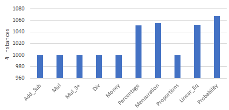
Figure 1: Distribution on different types of questions

4 Our Approach: Warm

We propose a weakly supervised model, Warm, for solving the MWP using only the answer for supervision. It is a two-step cascaded approach for weakly supervised MWP solving. For the first step, we propose a model that predicts the equation, given a problem text and answer. This model uses reinforcement learning to search the space of possible equations, given the question and the correct answer only. The answer acts as the goal of the agent and the search is terminated either when the answer is reached or when the equation length exceeds a pre-defined length (this is required, else the search space would be infinitely large). The model is designed to be a two layer bidirectional GRU (Cho et al., 2014) encoder and a decoder network with fully connected units (described in Section 4.3). We refer to this model as Warm. Note that this model requires an answer to determine when to stop exploring. Since we ultimately want a model which should only take the problem statement as input and generate the answer (by generating the correct equation), this model alone is insufficient for evaluation. Using this model, we create a noisy equation-annotated dataset from the weakly annotated training dataset (the training dataset has answers since it is weakly supervised). We use only those instances to create the dataset for which the equation generated by the model yields the correct answer. Note that the equations are noisy, since there is no guarantee that the generated equation will be the shortest or even correct. In the second step, we use this noisy data for supervised training of a state-of-the-art model. The trained supervised model is finally used for evaluation. For simplicity, we provide a summary of notations in Section 1 in supplementary.

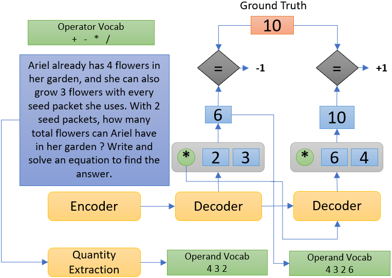
Figure 2: Inference Illustration

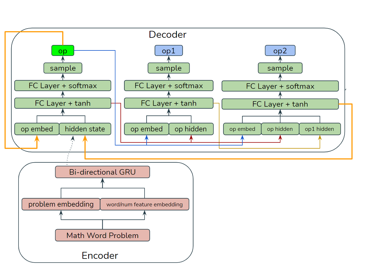
Figure 3: Architecture for generating equation tree in Warm.

4.1 Equation Generation

The first step of our approach is to generate equation given a problem text $P$ and answer $A$. This is done by using our Warm model. The problem text is passed through the encoder of the Warm model to get its encoded representation which is then fed to the decoder. At each time step, the decoder generates an operator and its two operands from the operator and operand vocabulary list. The operation is then executed to obtain a new quantity. This quantity is checked against the ground truth and if it matches the ground truth, the decoding is terminated and a reward of +1 is assigned. Else we assign a reward of -1 and the generated quantity is added to the operand vocabulary list and the decoding continues. The working of the Warm model and architecture are illustrated in Figure 2 and Figure 3 respectively. In the following few subsections, we describe the architecture as well as the training in details.

4.2 Encoder

The encoder takes as input, the MWP represented as a sequence of tokens $P=x_{1}x_{2}x_{3}...x_{n}$. We replace each number in the question with a special token $<num\_j>$ to obtain this sequence where $j$ denotes the index of number in the operand vocab for that question. Each word token $x_{i}$ is first transformed into the corresponding word embedding $\boldsymbol{x}_{i}$ by looking up an embedding matrix $\boldsymbol{M}_{w}$. Next, a binary feature is appended to the embedding to indicate whether the token is a word or a number. As depicted in the lower half of Figure 3, this appended embedding vector is then passed through a 2 layer bidirectional GRU (Cho et al., 2014) and the outputs from both directions of the final layer are summed to get the encoded representation of the text. This representation is then passed on to the decoder.

4.3 Decoder

The decoder consists of 3 fully connected networks for generating operator, left operand and the right operand. As illustrated in the upper half of Figure 3, the decoder takes as input the previous decoded operand and the last decoder hidden state and outputs the operator, left operand, right operand and hidden state at the current time step. We initialize the decoder hidden state with the last state of the encoder:

$o^{p}_{t},o^{l}_{t},o^{r}_{t},h^{d}_{t}=DecoderFCN(o^{p}_{t-1},h^{d}_{t-1})$

Here, $h^{d}_{t}$ is the decoder hidden state at the $t^{th}$ time step. $o^{p}_{t}$, $o^{l}_{t}$ and $o^{r}_{t}$ are probability distributions over operators, left and right operands respectively.

4.3.1 Operator generation

Inside our decoder, we learn an operator embedding matrix $Em_{op}(op_{t-1})$, where $op_{t-1}$ is the operator sampled in the last time step. We generate the operator hidden state $h^{op}_{t}$ using a gating mechanism.

$$g^{op}_{t}=\sigma(W^{1}_{op}[Em_{op}(op_{t-1});h^{d}_{t-1}]+b^{1}_{op})$$

$$h^{op}_{t}=g^{op}_{t}*tanh(W^{2}_{op}[Em_{op}(op_{t-1});h^{d}_{t-1}]+b^{2}_{op})$$

$$o^{p}_{t}=softmax(W^{3}_{op}h^{op}_{t}+b^{3}_{op})$$

Here $\sigma()$ denotes the sigmoid function and $*$ denotes elementwise multiplication. We sample operator $op_{t}$ from the probability distribution $o^{p}_{t}$.

4.3.2 Left Operand Generation

We use the embedding of the current operator $Em(op_{t})$ and the operator hidden state $h^{op}_{t}$ to obtain a probability distribution over the operands. We employ a similar gating mechanism as used for generating operator.

$$g^{ol}_{t}=\sigma(W^{1}_{ol}[Em_{op}(op_{t});h^{op}_{t}]+b^{1}_{ol})$$

$$h^{ol}_{t}=g^{ol}_{t}*tanh(W^{2}_{ol}[Em_{op}(op_{t});h^{op}_{t}]+b^{2}_{ol})$$

$$o^{l}_{t}=softmax(W^{3}_{ol}h^{ol}_{t}+b^{3}_{ol})$$

We sample the left operand $ol_{t}$ from the probability distribution $o^{l}_{t}$.

4.3.3 Right Operand Generation

For generating the right operand, we use the additional context information that is already available from the generated left operand. Thus, in addition to the operator embedding $Em_{op}(op_{t})$ and operator hidden state $h^{op}_{t}$ we also use the left operand hidden state to get the right operand hidden state $h^{or}_{t}$.

$$g^{or}_{t}=\sigma(W^{1}_{or}[Em_{op}(op_{t});h^{op}_{t};h^{ol}_{t}]+b^{1}_{or})$$

$$h^{or}_{t}=g^{or}_{t}*tanh(W^{2}_{or}[Em_{op}(op_{t});h^{op}_{t};h^{ol}_{t}]+b^{2}_{or})$$

$$o^{r}_{t}=softmax(W^{3}_{or}h^{or}_{t}+b^{3}_{or})$$

We sample the right operand $or_{t}$ from the probability distribution $o^{l}_{t}$. The hidden state $h^{or}_{t}$ is returned as the current decoder state $h^{d}_{t}$.

4.3.4 Bottom-up Equation Construction

For each training instance, we maintain a dictionary of possible operands $OpDict$. Initially, this dictionary contains the numeric values from the instance, i.e., the number tokens we have replaced with $<num\_j>$ during encoding. At the $t^{th}$ decoding step, we sample an operator $op_{t}$, left operand $ol_{t}$ and right operand $or_{t}$. We get an intermediate result by using the operator corresponding to $op_{t}$ on the operands $ol_{t}$ and $or_{t}$. This intermediate result is added to $OpDict$ which enables us to reuse the results of previous computations in future decoding steps. Thus, $OpDict$ acts as a dynamic dictionary of operands and we use it to progress towards the final answer in a bottom-up manner.

4.4 Rewards and Loss

We use the REINFORCE (Williams, 1992) algorithm for training the model using just the final answer as the ground truth. We model the reward as $+1$ if the predicted answer matches the ground truth and $-1$ if the predicted answer does not equal the ground truth.

Let $R_{t}$ be defined as the reward obtained after generating $y_{t}=(op_{t},o_{l},o_{r})$. The probability $P_{t}$ of generating the tuple $y_{t}$ is specified by $p_{\theta}(y_{t})=\prod\limits_{i=1}^{t}o^{p}_{i}\times o^{l}_{i}\times o^{r}_{i}$. The loss is specified as $L=-\sum\limits_{i}\mathbb{E}_{p_{\theta}(y_{i})}[R_{i}]$ and the corresponding gradient is $\nabla_{\theta}L=\sum\limits_{i}\sum\limits_{y_{i}}p_{\theta}(y_{i})R_{i}\nabla_{\theta}\log p_{\theta}(y_{i})$.

Since the space of $y_{i}$ makes it infeasible to compute the exact gradient, we use the standardized technique of sampling $y_{i}$ from $p_{\theta}(y_{i})$ to obtain an estimate of the gradient.

4.5 Beam Exploration in Training

Since the reward space for our problem is very sparse, we observe that during model training, the gradients go to zero. Our model converges too quickly to some local optima and consequently, the training accuracy saturates to some fixed value despite performing training for a large number of epochs. In order to counter this problem, we employ beam exploration in the training procedure. Instead of sampling operator $op_{t}$, left operand $ol_{t}$ and right operand $or_{t}$ only once in each decoding step, we sample $w$ triplets $(op_{t},ol_{t},or_{t})$ without replacement from the joint probability space in each decoding step. Here $w$ is the beam width. This helps in exploring $w$ different paths each epoch, thus increasing the exploration capabilities and reduce the problem of cold start. In order to select beams from all possible candidates, we have tried multiple heuristics by inspecting the probability and reward values. We have observed empirically that selecting the beam that gives a positive reward at the earliest decoding step yields the best performance. This enables our model to explore more and mitigates the above problem significantly.

4.6 Warm-S: Adding Semi-supervision

While it is expensive to completely label large MWP datasets with equations, it is relatively easier to annotate a small percentage of that data. We argue that addition of this small amount of semi-supervision can improve the model training significantly.

We, therefore, consider a model that benefits from a relatively small amount of strong supervision in the form of equation annotated data: $D_{s}$, in addition to a potentially larger sized math problem datasets with only weak supervision $D_{w}$. For a data instance $d$: $d.p$, $d.e$, and $d.a$ represent its problem statement, equation, and answer respectively. $D_{s}$ consists of instances of the form $(d.p,d.e,d.a)$ while $D_{w}$ contains instances of the form $(d.p,d.a)$. We extend the Warm model to include a Cross-Entropy loss component for instances belonging to $D_{s}$. The net loss is the sum of the REINFORCE ($RL_{\mbox{{Warm}}}$) and Cross-Entropy losses shown below:-

Loss 1:$\sum\limits_{d\in D_{w}}RL_{\mbox{{Warm}}}(d.p,d.a)$

Loss 2: $\sum\limits_{d\in D_{s}}Cross\_Entropy(d.e,$

$\mbox{{Warm}}(d.p,d.a))$

Thus, we facilitate semi-supervision through Loss 2. That is, we jointly use the equations predicted (by Warm) for datapoints belonging to $D_{w}$ and the ground truth equations for instances belonging to $D_{s}$, for training any state-of-the-art supervised MWP solver.

5 Experimental Setup

In this section, we report details of the experiments on four datasets to examine the performance of the proposed weakly supervised model Warm and its semi-supervised extension Warm-S. We present comparisons with various baselines as well as with fully supervised models.

5.1 Datasets

We perform all our experiments on the publicly available AllArith (Roy and Roth, 2017) and Math23K (Wang et al., 2017) datasets and also on our EW10K and HW10K datasets.For each dataset, we have used a $80:20$ train-test split.
AllArith contains 831 MWPs, annotated with equations and answers. It is populated by collecting problems from smaller datasets, viz., AI2 (Hosseini et al., 2014), IL (Roy and Roth, 2015), CC (Roy and Roth, 2015) and SingleEQ (Koncel-Kedziorski et al., 2015). All mentions of quantities are normalized to digits. Further, near-duplicate problems (with over 80% match of unigrams and bigrams) are filtered out.
Math23K (Wang et al., 2017) contains 23,161 MWPs in Chinese with 2187 templates, annotated with equations and answers, for elementary school students and is crawled from multiple online education websites. It is the largest publicly available dataset for the task of automatic MWP solving.
EW10K (c.f., Section 3) contains 10,227 MWPs in English and HW10K contains 9,896 in Hindi for classes VI to X. We employ a $80:20$ train-test split in each case.

5.2 Dataset Preprocessing

We replace every number token in the problem text with a special word token $<num\_j>$ before providing it as input to the encoder. We also define a set of numerical constants $V_{const}$ to solve those problems which might require special numeric values that may not be present in the problem text. For example, consider the problem “The radius of a circle is 2.5, what is its area?”, the solution is “$\pi$ x 2.5 x 2.5”, but the constant quantity $\pi$ cannot be found in the text. As our model does not use equations as supervision, we cannot know precisely what extra numeric values might be required for a problem, so we fix $V_{const}=\{1,\pi\}$. Finally, the operand dictionary for every problem is initialised as $OpDict=n_{P}\cup V_{const}$ where $n_{P}$ is the set of numeric values present in the problem text.

5.3 Implementation Details

We implement all our models in PyTorch (Paszke et al., 2019). We set the dimension of the word embedding layer to 128, and the dimension of the hidden states for other layers to 512. We use the REINFORCE (Williams, 1992) algorithm and Adam (Kingma and Ba, 2014) to optimize the parameters. The initial value of the learning rate is set to 0.001, and the learning rate is multiplied by 0.7 every 75 epochs. We also set the dropout probability to 0.5 and weight decay to 1e-5 to avoid over-fitting. Finally, we set the beam width to 5 in beam exploration.We train our model for 200 epochs with the batch size set to 256.

5.4 Models

We compare the MWP solving accuracy of our weakly supervised models with beam exploration on the following set of baseline and fully supervised models:

Warm is the proposed weakly supervised approach to equation generation (described from Section 4.1 until 4.4) by employing beam exploration (c.f., Section 4.5).
Warm w/o Beam Exploration is Warm without beam exploration while decoding.
Warm-S is the semi-supervised extension to Warm (c.f., Section 4.6) using beam exploration (Section 4.5).

Warm-S w/o Beam Exploration is the same as Warm-S but does not use beam exploration while decoding.
Random Equation Sampling consists of a random search over $k$ parallel paths of length $d$. For each path, an operator and its two operands are uniformly sampled from the given vocabulary and the result is added to the operand vocabulary (similar to Warm). The equation is terminated once the correct answer is reached. We set $k=5$ and $d=40$ for a fair comparison with our model in terms of the number of search operations.
Seq2Seq Baseline is a GRU (Cho et al., 2014) based seq2seq encoder-decoder model. REINFORCE (Williams, 1992) is used to train the model. Beam exploration is also employed to mitigates issues mentioned in Section 4.5.
LBF (Hong et al., 2021) is a weakly supervised model which uses only answer as supervision by fixing incorrect equation parse trees in each iteration. It subsequently performs training with the fixed trees.
Hybrid model w/ SNI (Wang et al., 2017) is a combination of the retrieval and the RNN-based Seq2Seq models with significant number identification (SNI).
Ensemble model w/ EN (Wang et al., 2018a) is an ensemble model that selects the result according to generation probability across Bi-LSTM, ConvS2S and Transformer Seq2Seq models with equation normalization (EN).
Semantically-Aligned (Chiang and Chen, 2019) is a Seq2Seq model with an encoder designed to understand the semantics of the problem text and a decoder equipped with a stack to facilitate tracking the semantic meanings of the operands.
T-RNN + Retrieval (Wang et al., 2019) is a combination of the retrieval model and the T-RNN model comprising a structure prediction module that predicts the template with unknown operators and an answer generation module that predicts the operators.
Seq2Tree (Liu et al., 2019) is a Seq2Tree model with a Bi-LSTM encoder and a top-down hierarchical tree-structured decoder consisting of an LSTM that makes use of the parent and sibling information fed as the input.

GTS (Xie and Sun, 2019) is a tree-structured neural model that generates the expression tree in a goal-driven manner.

Graph2Tree (Zhang et al., 2020) consists of a graph-based encoder which captures the relationships and order information among the quantities. It also employs a tree-based decoder that generates the expression tree in a goal-driven manner.

As described earlier in Section 4, we use our weakly supervised models (Warm and Warm-S) to generate labelled data (i.e., equations) which we then use to train a supervised model. We have performed experiments using GTS (Xie and Sun, 2019) and Graph2Tree (Zhang et al., 2020) as the supervised models since they are the current state-of-the-art.

6 Results and Analysis

Weakly Supervised Models	AllArith	Math23K	EW10K	HW10K
Warm w/o Beam Exploration	42.1	14.5	57.5	67.3
Warm	97.4	93.8	99.3	99.5
Baselines	AllArith	Math23K	EW10K	HW10K
Random Equation Sampling	53.4	17.6	46.3	66.6
Seq2Seq Baseline	67.0	7.1	77.6	75.8

Table 2: Equation generation accuracies of Warm based models compared to baselines. All models are trained using ground truth answers on the training set. Warm outperforms all the remaining models by as significant margin on all the datasets. Evidently, beam exploration significantly improves performance.

Weakly Supervised Models	AllArith	Math23K	EW10K	HW10K
Warm w/o Beam Exploration(GTS)	36.1	12.8	52.6	54.1
Warm (GTS)	66.9	55.3	86.9	81.5
Warm w/o Beam Exploration(Graph2Tree)	48.2	13.5	49.8	58.3
Warm (Graph2Tree)	68.7	56.0	87.2	82.9
LBF ‡	51.8	53.6	81.3	75.8
Fully Supervised Models	AllArith	Math23K	EW10K	HW10K
Graph2Tree‡	71.9	75.5	NA	NA
GTS‡	70.5	73.6	NA	NA
Seq2Tree	–	69.0	NA	NA
T-RNN + Retrieval	–	68.7	NA	NA
Semantically-Aligned†	–	65.8	NA	NA
Ensemble model w/ EN	–	68.4	NA	NA
Hybrid model w/ SNI†	–	64.7	NA	NA

Table 3: MWP solving accuracy of Warm-based models compared to various supervised models on AllArith and Math23K datasets. $\dagger$ denotes that result was reported on 5-fold cross validation. All other models are tested on the test set. $\ddagger$ denotes that the result is on the same train-test split as ours. “–” denotes code unavailability/reproducibility issues. NA is not applicable.

Problem: Ariel already has 4.0 flowers in her garden, and she can also grow 3.0 flowers with every seed packet she uses. With 2.0 seed packets, how many total flowers can Ariel have in her garden ?
Answer: 10.0
Equation Generated: X=(4.0+(2.0*3.0)) (Correct)
Problem: Celine took a total of 6.0 quizzes over the course of 3.0 weeks. After attending 7.0 weeks of school this quarter, how many quizzes will Celine have taken in total ? Assume the relationship is directly proportional.
Answer: 14.0
Equation Generated: X=(7.0+7.0) (Incorrect)

Table 4: Equation Generated by Warm model

Problem: Latrell ordered a set of yellow and purple pins. He received 72.0 yellow pins and 8.0 purple pins. What percentage of the pins were yellow?
Equation Generated by WARM (G2T): X=(72.0*(100.0/(72.0+8.0)))(Correct)
Equation Generated by LBF: X=(1.0+(1.0+72.0)) (Incorrect)
Problem: A square barn has a perimeter of 28.0 metres. How long is each side of the barn ?
Equation Generated by WARM(G2T): X=((28.0/2.0)/2.0) (Correct)
Equation Generated by LBF: X=((28.0+28.0)/28.0) (Incorrect)

Table 5: Comparing Warm and LBF model predicted equations

6.1 Analyzing Warm

In Table 2, we observe that our model Warm yields far higher accuracy than random baselines with the accuracy values close to 100% on AllArith and EW10K. Thus we are able to more accurately generate equations for a given problem and answer which can then be used to train supervised models. Please note that, in Table 2, we report equation generation accuracies on the training set by training the weakly supervised and baseline models using ground truth answers on the training set.

As has been discussed earlier in Section 4.5, our model Warm w/o Beam Exploration suffers from the problem of converging to local optima because of the sparsity of the reward signal. Training our weakly supervised models with beam exploration alleviates the issue to a large extent as we explore the solution space much more extensively and thus partly circumventing the sparsity issue. We observe vast improvement in the training accuracy by introduction of beam exploration. The model Warm yields training accuracy significantly higher than its non-beam-explore counterpart. Warm yields the best training accuracy overall. Since the equation generation accuracies of the baselines reported in Table 2 are far worse,the MWP solving accuracies turn out to be significantly worse - around 8-10%, and hence we do not report them.

We also observe that Warm yields results comparable to the various supervised models without requiring any supervision from gold equations. On AllArith, Warm achieves an accuracy of 66.9% and 68.7% using GTS and Graph2Tree as the supervised models respectively. The state-of-the-art supervised model Graph2Tree yields 71.9%. On Math23k, the difference between Warm and the supervised models is more pronounced. Warm’s performance is comparable to that of LBF on Math23k but significantly better on AllArith, EW10Kand HW10K, as evident in Table 3. We have shown a comparison of predicted equations by LBF and Warm in Table 5

In Table 4, we present some predictions. As can be seen, the model is capable of producing long complex equations as well. Sometimes, it may reach the correct answer but through an incorrect equation. E.g.: In the last example, the correct equation would have been $X=7.0*6.0/3.0$, but the model predicted $X=7.0+7.0$.

6.2 Analysing Semi-supervision through Warm-S

For analyzing semi-supervision, we combined AllArith (831) with EW10K (10227). We randomly sampled 80% of this data (8846) as our train-set. In retrospect, our train-set consists of 560 instances from AllArith that are completely labelled (amounting to 6.3% of the train-set). We compare our semi-supervised approach against the weakly supervised approach, wherein the entire training data is treated as having only answer labels.

In Table 6, we observe that with less than 10% of fully annotated data, our equation exploration accuracy increases from 56.7% to 92.0% without beam exploration and 99.0% to 99.2% with beam exploration. In Table 7, we also observe a similar trend while training the supervised models; our final MWP solving accuracy increases from 51.2% to 87.4% for Warm w/o Beam Exploration and Graph2Tree as the supervised model. We also study thethere effect of varying amount of complete supervision in Supplementary Section:2.

Weakly Supervised Models	AllArith +EW10K
Warm w/o Beam Exploration	56.7
Warm	99.0
Semi Supervised Models	AllArith+EW10K
Warm-S w/o Beam Exploration	92.0
Warm-S	99.2

Table 6: Equation generation accuracy of Warm-S compared to weakly supervised models and baselines.

Weakly Supervised Models	AllArith +EW10K
Warm w/o Beam Exploration(GTS)	50.2
Warm (GTS)	87.2
Warm w/o Beam Exploration(Graph2Tree)	51.2
Warm (Graph2Tree)	87.8
Semi Supervised Models	AllArith+EW10K
Warm-S w/o Beam Exploration(GTS)	87.2
Warm-S (GTS)	92.1
Warm-S w/o Beam Exploration(Graph2Tree)	87.4
Warm-S (Graph2Tree)	93.6

Table 7: MWP solving accuracy of Warm-S compared to Warm. With semi-supervision, there is a significant increase in accuracy for Warm w/o Beam Exploration, bringing its performance closer to Warm.

7 Conclusion

We have proposed a two step approach to solving math word problems, using only the final answer for supervision. Our weakly supervised approach, Warm, achieves a reasonable accuracy of 56.0 on the standard Math23K dataset even without leveraging equations for supervision. We also curate and release large scale MWP datasets, EW10K, in English and HW10K, in Hindi. We observed that the results are encouraging for simpler MWPs. We also present the benefits of incorporating a semi-supervised extension to Warm.

Appendix A Appendix

A.1 Notations

We summarize the notations used in section 4 of the main paper in table 8.

Notation	Description
$W$	Weight of the FC layers.
$o^{p}_{t}$	Probability distribution of operators at decoding timestep t.
$o^{l}_{t}$	Probability distribution of the left operand at decoding timestep t.
$o^{r}_{t}$	Probability distribution of the right operand at decoding timestep t.
$h^{d}_{t}$	Decoder hidden state at timestep t.
$Em_{op}$	Operator Embedding Matrix
$h^{op}_{t}$	Hidden state for the operator at timestep t
$op_{t}$	Operator sampled from $o^{p}_{t}$.
$h^{ol}_{t}$	Hidden state for the left operand at timestep t.
$ol_{t}$	Left operand sampled from $o^{l}_{t}$.
$h^{or}_{t}$	Hidden state for the right operator at timestep t.
$or_{t}$	Right operator sampled from $o^{r}_{t}$.
OpDict	Operand dictionary used while decoding
$R_{t}$	Rewards obtained at timestep t.
$p_{\theta}(y_{t})$	Probability of generating $y_{t}=(op_{t},ol_{t},or_{t})$ at timestep t.

Table 8: Summary of notation used.

A.2 Ablation Study: Varying Amount of Semi-supervision

We performed an experiment to study the effect of different amounts of supervision by varying the number of instances in training set we treat as fully labelled. The number of fully labelled instances is X-axis*80. We observe that just having 160 equation-labelled instances (out of 8846 ie. 1.8%) improves the equation-exploration accuracy significantly (46.7% to 90.6%) when we don’t use beam exploration.

Figure 4: Equation Exploration accuracy with varying supervision

A.3 Infrastructre Details

GPU Model used :
1)Model number: GeForce GTX 1080 Ti
2)Memory : 12GB

Training time :
1) WARM takes 4 hours for training
2) G2T takes 1 hour and 30 minutes to get trained completely

References

- Akula et al. (2021) Jayaprakash Akula, Rishabh Dabral, Preethi Jyothi, and Ganesh Ramakrishnan. 2021. Cross lingual video and text retrieval: A new benchmark dataset and algorithm. In Proceedings of the 2021 International Conference on Multimodal Interaction, pages 595–603.
- Amini et al. (2019) Aida Amini, Saadia Gabriel, Peter Lin, Rik Koncel-Kedziorski, Yejin Choi, and Hannaneh Hajishirzi. 2019. Mathqa: Towards interpretable math word problem solving with operation-based formalisms. arXiv preprint arXiv:1905.13319.
- Bakman (2007) Yefim Bakman. 2007. Robust understanding of word problems with extraneous information. arXiv preprint math/0701393.
- Chiang and Chen (2019) Ting-Rui Chiang and Yun-Nung Chen. 2019. Semantically-aligned equation generation for solving and reasoning math word problems. In Proceedings of the 2019 Conference of the North American Chapter of the Association for Computational Linguistics: Human Language Technologies. ACL.
- Cho et al. (2014) Kyunghyun Cho, Bart van Merriënboer, Caglar Gulcehre, Dzmitry Bahdanau, Fethi Bougares, Holger Schwenk, and Yoshua Bengio. 2014. Learning phrase representations using RNN encoder–decoder for statistical machine translation. In Proceedings of the 2014 Conference on Empirical Methods in Natural Language Processing (EMNLP), pages 1724–1734, Doha, Qatar. Association for Computational Linguistics.
- Fletcher (1985) Charles R. Fletcher. 1985. Understanding and solving arithmetic word problems: A computer simulation. Behavior Research Methods, 17:565–571.
- Hong et al. (2021) Yining Hong, Qing Li, Daniel Ciao, Siyuan Haung, and Song-Chun Zhu. 2021. Learning by fixing: Solving math word problems with weak supervision.
- Hosseini et al. (2014) Mohammad Javad Hosseini, Hannaneh Hajishirzi, Oren Etzioni, and Nate Kushman. 2014. Learning to solve arithmetic word problems with verb categorization. In Proceedings of the 2014 Conference on Empirical Methods in Natural Language Processing (EMNLP), pages 523–533. ACL.
- Huang et al. (2018) Danqing Huang, Jing Liu, Chin-Yew Lin, and Jian Yin. 2018. Neural math word problem solver with reinforcement learning. In Proceedings of the 27th International Conference on Computational Linguistics, pages 213–223. ACL.
- Huang et al. (2016) Danqing Huang, Shuming Shi, Chin-Yew Lin, Jian Yin, and Wei-Ying Ma. 2016. How well do computers solve math word problems? large-scale dataset construction and evaluation. In Proceedings of the 54th Annual Meeting of the Association for Computational Linguistics (Volume 1: Long Papers), pages 887–896, Berlin, Germany. Association for Computational Linguistics.
- Kingma and Ba (2014) Diederik Kingma and Jimmy Ba. 2014. Adam: A method for stochastic optimization. International Conference on Learning Representations.
- Koncel-Kedziorski et al. (2015) Rik Koncel-Kedziorski, Hannaneh Hajishirzi, Ashish Sabharwal, Oren Etzioni, and Siena Dumas Ang. 2015. Parsing algebraic word problems into equations. Transactions of the Association for Computational Linguistics, 3:585–597.
- Kumar et al. (2019) Vishwajeet Kumar, Nitish Joshi, Arijit Mukherjee, Ganesh Ramakrishnan, and Preethi Jyothi. 2019. Cross-lingual training for automatic question generation. arXiv preprint arXiv:1906.02525.
- Kumar et al. (2015) Vishwajeet Kumar, Ashish Kulkarni, Pankaj Singh, Ganesh Ramakrishnan, and Ganesh Arnaal. 2015. A machine assisted human translation system for technical documents. In Proceedings of the 8th International Conference on Knowledge Capture, pages 1–5.
- Kumar et al. (2018) Vishwajeet Kumar, Ganesh Ramakrishnan, and Yuan-Fang Li. 2018. Putting the horse before the cart: A generator-evaluator framework for question generation from text. arXiv preprint arXiv:1808.04961.
- Kushman et al. (2014) Nate Kushman, Yoav Artzi, Luke Zettlemoyer, and Regina Barzilay. 2014. Learning to automatically solve algebra word problems. In Proceedings of the 52nd Annual Meeting of the Association for Computational Linguistics (Volume 1: Long Papers), pages 271–281. Association for Computational Linguistics.
- Liang et al. (2016a) Chao-Chun Liang, Kuang-Yi Hsu, Chien-Tsung Huang, Chung-Min Li, Shen-Yu Miao, and Keh-Yih Su. 2016a. A tag-based english math word problem solver with understanding, reasoning and explanation. In Proceedings of the Demonstrations Session, NAACL HLT 2016, pages 67–71. The Association for Computational Linguistics.
- Liang et al. (2016b) Chao-Chun Liang, Kuang-Yi Hsu, Chien-Tsung Huang, Chung-Min Li, Shen-Yu Miao, and Keh-Yih Su. 2016b. A tag-based statistical english math word problem solver with understanding, reasoning and explanation. In Proceedings of the Twenty-Fifth International Joint Conference on Artificial Intelligence, IJCAI’16, page 4254–4255. AAAI Press.
- Liu et al. (2019) Qianying Liu, Wenyv Guan, Sujian Li, and Daisuke Kawahara. 2019. Tree-structured decoding for solving math word problems. In Proceedings of the 2019 Conference on Empirical Methods in Natural Language Processing and the 9th International Joint Conference on Natural Language Processing (EMNLP-IJCNLP), pages 2370–2379.
- Mitra and Baral (2016) Arindam Mitra and Chitta Baral. 2016. Learning to use formulas to solve simple arithmetic problems. In Proceedings of the 54th Annual Meeting of the Association for Computational Linguistics (Volume 1: Long Papers), pages 2144–2153. Association for Computational Linguistics.
- Paszke et al. (2019) Adam Paszke, Sam Gross, Francisco Massa, Adam Lerer, James Bradbury, Gregory Chanan, Trevor Killeen, Zeming Lin, Natalia Gimelshein, Luca Antiga, Alban Desmaison, Andreas Köpf, Edward Yang, Zach DeVito, Martin Raison, Alykhan Tejani, Sasank Chilamkurthy, Benoit Steiner, Lu Fang, Junjie Bai, and Soumith Chintala. 2019. Pytorch: An imperative style, high-performance deep learning library.
- Roy and Roth (2015) Subhro Roy and Dan Roth. 2015. Solving general arithmetic word problems. In Proceedings of the 2015 Conference on Empirical Methods in Natural Language Processing, pages 1743–1752. ACL.
- Roy and Roth (2017) Subhro Roy and Dan Roth. 2017. Unit dependency graph and its application to arithmetic word problem solving. In Proceedings of the Thirty-First AAAI Conference on Artificial Intelligence, page 3082–3088. AAAI Press.
- Roy and Roth (2018) Subhro Roy and Dan Roth. 2018. Mapping to declarative knowledge for word problem solving. Trans. Assoc. Comput. Linguistics, 6:159–172.
- Roy et al. (2016) Subhro Roy, Shyam Upadhyay, and Dan Roth. 2016. Equation parsing : Mapping sentences to grounded equations. In Proceedings of the 2016 Conference on Empirical Methods in Natural Language Processing, EMNLP 2016, pages 1088–1097. The Association for Computational Linguistics.
- Shen et al. (2021) Jianhao Shen, Yichun Yin, Lin Li, Lifeng Shang, Xin Jiang, Ming Zhang, and Qun Liu. 2021. Generate & rank: A multi-task framework for math word problems. arXiv preprint arXiv:2109.03034.
- Singh et al. (2016) Pankaj Singh, Ashish Kulkarni, Himanshu Ojha, Vishwajeet Kumar, and Ganesh Ramakrishnan. 2016. Building compact lexicons for cross-domain smt by mining near-optimal pattern sets. In Pacific-Asia Conference on Knowledge Discovery and Data Mining, pages 290–303. Springer.
- Sundaram and Khemani (2015) Sowmya S Sundaram and Deepak Khemani. 2015. Natural language processing for solving simple word problems. In Proceedings of the 12th International Conference on Natural Language Processing, pages 394–402. NLP Association of India.
- Tarunesh et al. (2021) Ishan Tarunesh, Sushil Khyalia, Vishwajeet Kumar, Ganesh Ramakrishnan, and Preethi Jyothi. 2021. Meta-learning for effective multi-task and multilingual modelling. arXiv preprint arXiv:2101.10368.
- Thakoor et al. (2018) Shantanu Thakoor, Simoni Shah, Ganesh Ramakrishnan, and Amitabha Sanyal. 2018. Synthesis of programs from multimodal datasets. In Proceedings of the AAAI Conference on Artificial Intelligence, volume 32.
- Upadhyay et al. (2016) Shyam Upadhyay, Ming-Wei Chang, Kai-Wei Chang, and Wen-tau Yih. 2016. Learning from explicit and implicit supervision jointly for algebra word problems. In Proceedings of the 2016 Conference on Empirical Methods in Natural Language Processing, pages 297–306.
- Wang et al. (2018a) Lei Wang, Yan Wang, Deng Cai, Dongxiang Zhang, and Xiaojiang Liu. 2018a. Translating math word problem to expression tree. In Proceedings of the 2018 Conference on Empirical Methods in Natural Language Processing, pages 1064–1069. ACL.
- Wang et al. (2018b) Lei Wang, Dongxiang Zhang, Lianli Gao, Jingkuan Song, Long Guo, and Heng Tao Shen. 2018b. Mathdqn: Solving arithmetic word problems via deep reinforcement learning. In Proceedings of the Thirty-Second AAAI Conference on Artificial Intelligence, AAAI, pages 5545–5552. AAAI Press.
- Wang et al. (2019) Lei Wang, Dongxiang Zhang, Jipeng Zhang, Xing Xu, Lianli Gao, Bing Tian Dai, and Heng Tao Shen. 2019. Template-based math word problem solvers with recursive neural networks. In Proceedings of the Thirty-Third AAAI Conference on Artificial Intelligence, AAAI, pages 7144–7151. AAAI Press.
- Wang et al. (2017) Yan Wang, Xiaojiang Liu, and Shuming Shi. 2017. Deep neural solver for math word problems. In Proceedings of the 2017 Conference on Empirical Methods in Natural Language Processing, pages 845–854. ACL.
- Williams (1992) Ronald J. Williams. 1992. Simple statistical gradient-following algorithms for connectionist reinforcement learning. Mach. Learn., 8(3–4):229–256.
- Wu et al. (2021) Qinzhuo Wu, Qi Zhang, Zhongyu Wei, and Xuan-Jing Huang. 2021. Math word problem solving with explicit numerical values. In Proceedings of the 59th Annual Meeting of the Association for Computational Linguistics and the 11th International Joint Conference on Natural Language Processing (Volume 1: Long Papers), pages 5859–5869.
- Xie and Sun (2019) Zhipeng Xie and Shichao Sun. 2019. A goal-driven tree-structured neural model for math word problems. In Proceedings of the 28th International Joint Conference on Artificial Intelligence, pages 5299–5305. AAAI Press.
- Yuhui et al. (2010) M. Yuhui, Z. Ying, C. Guangzuo, R. Yun, and H. Ronghuai. 2010. Frame-based calculus of solving arithmetic multi-step addition and subtraction word problems. In 2010 Second International Workshop on Education Technology and Computer Science, volume 2, pages 476–479.
- Zhang et al. (2018) Dongxiang Zhang, Lei Wang, Nuo Xu, Bing Tian Dai, and Heng Tao Shen. 2018. The gap of semantic parsing: A survey on automatic math word problem solvers. CoRR, abs/1808.07290.
- Zhang et al. (2020) Jipeng Zhang, Lei Wang, Roy Ka-Wei Lee, Yi Bin, Yan Wang, Jie Shao, and Ee-Peng Lim. 2020. Graph-to-tree learning for solving math word problems. In Proceedings of the 58th Annual Meeting of the Association for Computational Linguistics, pages 3928–3937, Online. Association for Computational Linguistics.