The TopFlavor scheme in the context of $W^{\prime}$ searches at LHC

Abstract

Many extensions of the Standard Model predict the existence of new charged or neutral gauge bosons, with a wide variety of phenomenological implications depending on the model adopted. The search for such particles is extensively carried through at the Large Hadron Collider (LHC), and it is therefore of crucial importance to have for each proposed scenario quantitative predictions that can be matched to experiments. In this work we focus on the implications of one of these models, the TopFlavor Model, proposing a charged $\text{W}^{\prime}$ boson that has preferential couplings to the third generation fermions. We compare such predictions to the ones from the so called Sequential Standard Model (SSM), that is used as benchmark, being one of the simplest and most commonly considered models for searches at the LHC. We identify the parameter space still open for searches at the LHC, and we show that the cross sections for the processes $pp\to\text{W}^{\prime}\to\tau\nu$ and $pp\to\text{W}^{\prime}\to tb$ in the TF assume different values with respect to the SSM as a function of the particle mass and width, and that the TF has realizations that would not be allowed in the SSM and not yet excluded by data. This study makes the case for further searches at the LHC, and shows how a complete and systematic model independent analysis of $\text{W}^{\prime}$ boson phenomenology at colliders is essential to provide guidance for future searches.

I introduction

The Standard Model (SM) successfully describes three fundamental interactions, and its predictions are in excellent agreement with data. It is however known that, even putting aside gravitational interactions, the SM cannot be the ultimate fundamental theory. Among the main clues leading to such conclusion are the observation of baryon asymmetry, the neutrino oscillation phenomena, and the dark paradigm. The SM also presents issues of self-consistency, like the Higgs hierarchy problem, that, while not corresponding to a specific observation, undermine its robustness as a fundamental theory valid at all energy regimes. Finally, statistically significant evidence of Nature’s behavior deviating from the SM has been mounting over the recent years in several sectors of particle physics, and that could be explained in the context of new physics scenarios. In the b-physics sector, flavor anomalies have been spotted at b-factories, BaBar and Belle, and at LHCb in the D* babarlfvd ; bellelfvd ; lhcblfvd and K* babarlfvk ; bellelfvk ; lhcblfvk decay ratios, possibly pointing towards lepton flavor universality violation Hiller:2017bz . The anomalous magnetic moment of the muon ($g-2$) at Brookhaven National Laboratory Bennett_2006 and Fermilab National Accelerator Laboratory Abi:2021gix has also been found to deviate significantly from SM expectations.

All the above points to the fact that the SM must be extended by some new theory, that can be built with top-down as well as bottom-up approaches.

Examples of top-down approaches are several gauge extensions of the SM that are inspired by Grand Unified Theories like the Pati-Salam model pati1994lepton . This model is based on the gauge group $SU(4)_{c}\times SU(2)_{L}\times SU(2)_{R}$, also referred to as (4, 2, 2), which is a maximal subgroup of $SO(10)$ grand unification group. In a bottom-up approach, other gauge symmetries can be considered, like the left-right $SU(3)_{c}\times SU(2)_{L}\times SU(2)_{R}\times U(1)$, also referred to as L-R model rabindra1986unification ; Corrigan:2015kfu , and the $SU(3)_{c}\times SU(3)_{L}\times U(1)_{Y}$, also referred to as (3, 3, 1) model pisano19923 ; buras2013anatomy ; boucenna2015predicting ; cabarcas2010flavor ; cogollo2012novel . Other possibilities have been proposed, inspired by the extension of the Higgs sector rather than the introduction of new symmetries, like Little Higgs models goh2007little ; schmaltz2004simplest ; Antipin_2013 and Twin Higgs models ahmed2018heavy ; chacko2006twin . All these SM extensions have a common feature: the prediction of new $\text{W}^{\prime}$ and $\text{Z}^{\prime}$ gauge bosons, langacker2009physics in analogy with the W and Z gauge bosons of the SM. In the current letter, we will focus on $\text{W}^{\prime}$ boson phenomenology, giving an overview of the models that can foresee its introduction, and focusing on deriving measurable predictions on a specific one, named TopFlavor (TF) Model.

The paper is organized as follows: Section II serves as a brief overview on the most common $\text{W}^{\prime}$ models. In Section III we will introduce the general properties of the TF model studied in this work. In Section IV we report the phenomenological implications for collider searches with a comparison with the SSM case, and in Section V we draw quantitative predictions for LHC searches. In section  VI we report our conclusions.

II $\text{W}^{\prime}$ models overview

The couplings of $\text{W}^{\prime}$ with SM particles, fermions, scalars, and vectors, depend on the specific gauge model. The new gauge boson interactions with fermions can be written in a general way as

$$\begin{split}\mathcal{L}^{\rm eff}&=\frac{V_{f_{i}f_{j}}}{2\sqrt{2}}g_{w}\bar{f_{i}}\gamma_{\mu}[\alpha_{R}^{f_{i}f_{j}}(1+\gamma^{5})+\\ &+\alpha_{L}^{f_{i}f_{j}}(1-\gamma^{5})]W^{\prime\mu}f_{j}+h.c.,\end{split}$$ (1)

where $V_{f_{i}f_{j}}$ is the analogue of the Cabibbo-Kobayashi-Maskawa (CKM) matrix if $f_{i}$ ed $f_{j}$ represent quarks, while for leptons $V_{f_{i}f_{j}}=\delta_{ij}$ and $g_{w}$ is the coupling with the $\text{W}^{\prime}$ collaboration2012search .

The parameters $\alpha_{R}^{f_{i}f_{j}}$ and $\alpha_{L}^{f_{i}f_{j}}$ are free in a model independent analysis, while specific $\text{W}^{\prime}$-models correspond to specific choices them.

The sequential standard model (SSM) described in Ref. altarelli1989searching is defined to have the same couplings to fermions as the SM W boson, leading to $g_{w}=e/\sin\theta_{W}$, $\alpha_{L}^{f_{i}f_{j}}=1$, and $\alpha_{R}^{f_{i}f_{j}}=0$ for $i,j=1,2,3$. It is worth mentioning that the SSM is not expected in the context of any gauge theory unless new scalars and fermions are assumed to extend the SM beside the $\text{W}^{\prime}$ boson langacker2009physics . Indeed the inclusion of a new $\text{W}^{\prime}$ boson requires to extend the gauge group with, for instance, an extra $SU_{\rm new}(2)$ group. In order to couple to the $\text{W}^{\prime}$ boson, the SM fermions, both quarks and leptons, must transform under the new $SU_{\rm new}(2)$. The minimal extension of the weak gauge group by means of a new $U(1)$ provides no $\text{W}^{\prime}$ boson, but gives a $\text{Z}^{\prime}$ one. Another feature of these models is that they require new scalar fields, since it is necessary to reproduce the SM with a spontaneous symmetry breaking (SSB) of the new symmetry group.

LR gauge models provide a possible example of such an extension, based on the $SU(2)_{L}\times SU(2)_{R}\times U(1)$ gauge group rabindra1986unification ; Corrigan:2015kfu , and give $\alpha_{R}^{f_{i}f_{j}}=\alpha_{R}$ and $\alpha_{L}^{f_{i}f_{j}}=\alpha_{L}$ where $\alpha_{L,R}$ are arbitrary parameters.

Another possible extension is the class of models based on a (3, 3, 1) gauge symmetry. In this case, the $\alpha_{R}^{f_{i}f_{j}}$ and $\alpha_{L}^{f_{i}f_{j}}$ assignment depends on the details of the model. In fact, within the (3, 3, 1) model there is some arbitrariness in the assignment of the matter field in order to complete the irreducible representation of $SU(3)_{L}$, namely the anti-triplet $\overline{\bf 3}$. However most of (3, 3, 1) models provide $\alpha_{L}^{f_{i}f_{j}}\neq 0$ and $\alpha_{R}^{f_{i}f_{j}}=0$ in analogy with the SSM. For instance, the Lagrangian of the model presented in Ref. pisano19923 contains

$$\begin{split}\mathcal{L}\supset&-\frac{g}{\sqrt{2}}(\bar{\ell}_{L}^{c}\gamma^{\mu}\nu_{\ell\,L}\text{W}^{\prime\,+}_{\mu}+\bar{J}_{1\,L}\gamma^{\mu}u_{L}\text{W}^{\prime\,+}_{\mu}\\ &-\bar{q}_{i\,L}\gamma^{\mu}J_{i\,L}\text{W}^{\prime\,+}_{\mu}+h.c.)\,,\end{split}$$ (2)

where $g=e\sqrt{1+3\sin^{2}\theta}/\sin\theta$, $\tan^{2}\theta\approx 11/6$, i=2,3, and $J_{1,2,3}$ are new quarks with exotic charges. It is important to notice that the quarks in the Lagrangian of Eq. (2) are not the mass eigenstates.

In conclusion, the effective Lagrangian reported in Eq. (1) is the most general one that parametrises the coupling of a $\text{W}^{\prime}$ boson with fermions. Nevertheless it is not satisfactory from a theoretical point of view in its most general form. To compute phenomenological, observable predictions, one must often reduce to a subset of parameters compatible with the conditions listed above.

In particular, for what concerns couplings to fermions, experimental searches often focus on two benchmark cases:

$$\text{W}^{\prime}_{L}: \quad\alpha_{L}^{f_{i}f_{j}}=1\,,\quad\alpha_{R}^{f_{i}f_{j}}=0\,,$$

$$\text{W}^{\prime}_{R}: \quad\alpha_{L}^{f_{i}f_{j}}=0\,,\quad\alpha_{R}^{f_{i}f_{j}}=1\,,$$ (3)

both of them have $g_{w}=e/\sin\theta_{W}$. While the first case is exactly the SSM introduced in Ref. altarelli1989searching , the second one is its right-handed version that is a special case of the LR model. The two cases in Eq. (3) do not cover the full extent of possible models that could actually appear in Nature. Other combinations of parameters could be allowed, motivated by different theoretical models or assumptions, resulting in a wider parameter space to explore at the LHC or future colliders.

In this work, we will explore the phenomenological implications of a third class of $\text{W}^{\prime}$ models, denoted as TopFlavor Model li1993gauge ; malkawi1996model , whose key assumptions are significantly different with respect to the ones leading to Eq. (3). In particular, we will show how a vast portion of the parameter space available to this model is not yet excluded by the LHC. We will evaluate the production rate of $pp\to\text{W}^{\prime}\to\tau\nu$ and $pp\to\text{W}^{\prime}\to tb$ processes, showing that it can range down to approximately a fifth of the one of the SSM.

III TopFlavor model

The most general realization of TF model is based on the gauge group PhysRevLett.47.1788 :

$$SU(3)_{C}\times SU(2)_{1}\times SU(2)_{2}\times SU(2)_{3}\times U(1)_{Y}\,,$$ (4)

where the $i^{th}$ flavor generation transforms as a doublet under $SU(2)_{i}$ and as a singlet under the other $SU(2)_{j}$ with i,j in (1,2,3), and $i\neq j$. The presence of three separate gauge groups for each family leaves considerable freedom in the realization of the TF model. In this work, we consider the one given in Refs. lee1998phenomenological ; Muller_1996 ; cao2016interpreting ; muller1997separate ; PhysRevLett.47.1788 ; li1993gauge , where the first two generations transform under the same $SU(2)_{12}$ and the third family, the heaviest one, transforms under $SU(2)_{3}$. Under such assumption, the gauge group reported in Eq. (4) reduces to:

$$SU(3)_{C}\times SU(2)_{12}\times SU(2)_{3}\times U(1)_{Y}\,.$$ (5)

Such a group can be obtained from the more general one in Eq. (4) by a SSB mechanism PhysRevLett.47.1788 . The model also requires to extend the scalar sector with two new fields: $\Phi$, that transforms as a doublet under $SU(2)_{12}$, and $\Sigma$, that is a bi-doublet under $SU(2)_{12}\times SU(2)_{3}$. We can write the bi-doublet scalar fields as:

$$\Sigma=\left(\begin{array}[]{cc}\sigma+i\pi_{3}&i\pi_{1}+\pi_{2}\\ i\pi_{1}-\pi_{2}&\sigma-i\pi_{3}\end{array}\right),$$ (6)

where $\pi^{i}$ and $\sigma$ are real fields, and the doublet scalar field as:

$$\Phi=\left(\begin{array}[]{c}\Phi^{+}\\ \Phi^{0}\end{array}\right).$$ (7)

The transformation rules of these fields are:

$$\begin{split}&\Sigma\to g_{12}\,\Sigma\,g_{3}^{\dagger},\\ &\Phi\to g_{12}\,g_{Y}\,\Phi,\end{split}$$ (8)

where $g_{12}\in SU(2)_{12}$, $g_{3}\in SU(2)_{3}$, and $g_{Y}\in U(1)_{Y}$.

Similarly to the SM, the degrees of freedom of all the real fields present in the scalar sector, except for $\text{Re}(\Phi^{0})$ and $\sigma$, are converted into the longitudinal component of the gauge bosons. The vacuum expectation values (v.e.v.s) of these fields are

$$\begin{split}\braket{\Sigma}&=\left(\begin{array}[]{cc}u&0\\ 0&u\end{array}\right),\quad\braket{\Phi}=\left(\begin{array}[]{c}0\\ v\end{array}\right),\end{split}$$ (9)

where both $v$ and $u$ are real numbers. The field $\Phi$ plays the same role as the Higgs field in the SM, with the difference that it couples to the third generation only.

The pattern of the SSB from the full symmetry group of Eq. (5) proceeds as follows: in the first step the field $\Sigma$ acquires its v.e.v. ($u\gg v$), leading to the SSB:

$$SU(2)_{12}\times SU(2)_{3}\xrightarrow{\Sigma}SU(2)_{L};$$ (10)

in the second step, the field $\Phi$ acquires its v.e.v. causing the SSB:

$$SU(2)_{L}\times U(1)_{Y}\xrightarrow{\Phi}U(1)_{EM},$$ (11)

which is the same breaking as in the SM.

The first two generations of leptons $L^{1,2}$ transform as $(2,1)$ under $SU(2)_{12}\times SU(2)_{3}$ while $L^{3}$ transforms as $(1,2)$. On the other hand, right handed leptons are singlets under $SU(2)_{12}\times SU(2)_{3}$. Similar assignments are given for quarks.

The model also contains seven gauge bosons, corresponding to the four SM gauge bosons and the new $\text{W}^{\prime}$ and $\text{Z}^{\prime}$ bosons.

The matter content of the model is summarized in Table 1.

	$SU(2)_{12}$	$SU(2)_{3}$	$U(1)_{Y}$
$L^{3}$	1	2	$-1/2$
$L^{1,2}$	2	1	$-1/2$
$Q^{3}$	1	2	$1/6$
$Q^{1,2}$	2	1	$1/6$
$u^{1,2,3}_{R}$	1	1	$2/3$
$d^{1,2,3}_{R}$	1	1	$-1/3$
$\ell^{1,2,3}_{R}$	1	1	$-1$
$\Sigma$	2	$2$	0
$\Phi$	1	2	$1/2$

Table 1: Matter content of the TopFlavor model.

Since the strong interaction sector does not change, we will omit its description.

The complete Lagrangian of the model is given for instance in Ref. malkawi2000light and is summarized here as:

$$\mathcal{L}=\mathcal{L}_{B}+\mathcal{L}_{F}+\mathcal{L}_{Y},$$ (12)

where $\mathcal{L}_{F}$ contains the fermion components, $\mathcal{L}_{B}$ contains the boson and scalar components , while $\mathcal{L}_{Y}$ contains the Yukawa interaction and is not reported here since it is model dependent and does not influence the phenomenological searches of $\text{W}^{\prime}$ at accelerators. $\mathcal{L}_{F}$ and $\mathcal{L}_{B}$ expressions are reported in the following:

$$\begin{split}&\mathcal{L}_{F}=i\bar{\Psi}\gamma^{\mu}D_{\mu}\Psi=\\ &i\bar{L}_{L}^{j}\gamma_{\mu}\left(\partial^{\mu}+i\frac{g_{12}}{2}\sigma^{i}W_{12}^{i\mu}-i\frac{g_{0}}{2}B^{\mu}\right)L_{L}^{j}+\\ +&i\bar{Q}_{L}^{j}\gamma_{\mu}\left(\partial^{\mu}+i\frac{g_{12}}{2}\sigma^{i}W_{12}^{i\mu}+i\frac{g_{0}}{6}B^{\mu}\right)Q_{L}^{j}+\\ +&i\bar{L}_{L}^{3}\gamma_{\mu}\left(\partial^{\mu}+i\frac{g_{3}}{2}\sigma^{i}W_{3}^{i\mu}-i\frac{g_{0}}{2}B^{\mu}\right)L_{L}^{3}+\\ +&i\bar{Q}_{L}^{3}\gamma_{\mu}\left(\partial^{\mu}+i\frac{g_{3}}{2}\sigma^{i}W_{3}^{i\mu}+\frac{g_{0}}{6}B^{\mu}\right)Q_{L}^{3}+\\ +&i\bar{u}_{R}^{\alpha}\gamma_{\mu}\left(\partial^{\mu}+\frac{2g_{0}}{3}B^{\mu}\right)u_{R}^{j}+\\ +&i\bar{d}_{R}^{\alpha}\gamma_{\mu}\left(\partial^{\mu}-i\frac{g_{0}}{3}B^{\mu}\right)d_{R}^{j}+\\ +&i\bar{e}_{R}^{\alpha}\gamma_{\mu}\left(\partial^{\mu}-ig_{0}B^{\mu}\right)e_{R}^{j},\end{split}$$ (13)

$$\begin{split}&\mathcal{L}_{B}=\frac{1}{2}D_{\mu}\Phi^{\dagger}D^{\mu}\Phi+\frac{1}{4}\rm{Tr}(D_{\mu}\Sigma^{\dagger}D^{\mu}\Sigma)+\\ &-V(\Sigma;\Phi)-\frac{1}{4}W^{a}_{12\mu\nu}W^{a\mu\nu}_{12}+\\ &-\frac{1}{4}W^{a}_{3\mu\nu}W^{a\mu\nu}_{3}-\frac{1}{4}B_{\mu\nu}B^{\mu\nu}\,,\end{split}$$ (14)

where $i=1,2$, $\alpha=1,2,3$, and the covariant derivative is defined as $D^{\mu}=\partial^{\mu}+ig_{12}\vec{T}\cdot\vec{W}_{12}^{\mu}+ig_{3}\vec{T}^{\prime}\cdot\vec{W}_{3}^{\mu}+ig_{0}YB^{\mu}$. Here $W_{3}^{1,2,3}$, $W_{12}^{1,2,3}$, and $B$ are the gauge bosons fields. As usual these can be written in terms of charged and neutral bosons $W_{3}^{\pm}$, $W_{12}^{\pm}$, $W_{3}^{0}$, $W_{12}^{0}$, and $B$. We also observe that the model has five free parameters, that are $u$, $v$, $g_{12}$, $g_{3}$, $g_{0}$.

The mass matrix of the charged bosons in the basis $W_{12}^{\pm}$, and $W_{3}^{\pm}$ is given by Muller_1996 :

$$\mathcal{M}_{1}=\left(\begin{array}[]{cc}\frac{g_{12}^{2}(u^{2}+v^{2})}{4}&-\frac{g_{12}g_{3}u^{2}}{4}\\ -\frac{g_{12}g_{3}u^{2}}{4}&\frac{g_{3}^{2}u^{2}}{4}\end{array}\right).$$ (15)

On the other hand, the neutral bosons mass matrix in the basis $B$, $W_{12}^{0}$, $W_{3}^{0}$ is given by:

$$\mathcal{M}_{2}=\left(\begin{array}[]{ccc}\frac{g_{0}^{2}v^{2}}{4}&-\frac{g_{12}g_{0}v^{2}}{4}&0\\ -\frac{g_{12}g_{0}v^{2}}{4}&\frac{g_{12}^{2}(v^{2}+u^{2})}{4}&-\frac{g_{12}g_{3}u^{2}}{4}\\ 0&-\frac{g_{12}g_{3}u^{2}}{4}&\frac{g_{3}^{2}u^{2}}{4}\end{array}\right)\,.$$ (16)

As expected, the matrix in Eq. (16) admits one massless eigenvalue, corresponding to the photon state. The diagonalisation of the matrix in Eq. (15) leads to a mixing between the charged bosons: the mixing angle between $W^{\pm}_{12}$ and $W^{\pm}_{3}$ will be denoted by $\theta^{\prime}$ in the following. Similarly, the diagonalisation of the matrix in Eq. (16) leads to a mixing between the neutral bosons: the mixing angle between $B$ and $W^{0}_{12}$ will be denoted by $\theta$. The requirement that the coupling between the photon and the charged leptons is equal to the electric charge leads to the following relations in the limit $u^{2}\gg v^{2}$:

$$\begin{split}g_{0}&=\frac{e}{\cos\theta}\,,\\ g_{12}&=\frac{e}{\sin\theta\cos\theta^{\prime}}\,,\\ g_{3}&=\frac{e}{\sin\theta\sin\theta^{\prime}}\,,\end{split}$$ (17)

where $e$ is the electric charge. The three couplings are therefore not linearly independent: we can rather use as free independent parameters the quantities $\theta$, $\theta^{\prime}$, $u$, and $v$. The eigenvalues of the charged and neutral gauge mass matrices are the physical masses of the bosons, which in the limit $u^{2}\gg v^{2}$ are:

$$\begin{split}M_{\text{W}}^{2}&\simeq\frac{v^{2}}{4}\frac{e^{2}}{\sin^{2}\theta}\left(1-\sin^{4}\theta^{\prime}\frac{v^{2}}{u^{2}}\right)\,,\\ M_{\text{Z}}^{2}&\simeq\frac{v^{2}}{4}\frac{e^{2}}{\sin^{2}\theta\cos^{2}\theta}\left(1-\sin^{4}\theta^{\prime}\frac{v^{2}}{u^{2}}\right)\,,\\ M_{\text{Z}^{\prime}}^{2}&\simeq M_{\text{W}^{\prime}}^{2}\simeq\\ &\frac{e^{2}v^{2}}{4\sin^{2}\theta}\left(\tan^{2}\theta^{\prime}+\frac{u^{2}}{v^{2}\sin^{2}\theta^{\prime}\cos^{2}\theta^{\prime}}\right)\,.\end{split}$$ (18)

We require that the masses of the W and Z bosons agree with the experimental values, namely $M_{\text{W}}=80.379\pm 0.012$ GeV and $M_{\text{W}}/M_{\text{Z}}=0.88147\pm 0.00013$ PDG . This requirement leads to:

$$\begin{array}[]{c}\sin^{2}\theta\simeq\sin^{2}\theta_{W}=0.23,\\ v\simeq v_{SM}\simeq 246\,\text{GeV},\end{array}$$ (19)

where $\theta_{W}$ is the Weinberg angle, and $v_{SM}$ is the v.e.v. of the SM. These relations impose two new constraints on the four free parameters $\theta$, $\theta^{\prime}$, $u$ and $v$: in the end we are left with two free parameters, namely $u$ and $\theta^{\prime}$.

Since our aim is to discuss the production of $tb$ and $\tau\nu_{\tau}$ via virtual $\text{W}^{\prime}$ boson decay, we give the interaction term between the leptons and the charged bosons as:

$$\begin{split}&\mathcal{L}\supset\frac{1}{\sqrt{2}}[h_{I,II}\left(e_{L}\gamma^{\mu}\text{W}_{\mu}^{-}\nu_{e\,L}+\mu_{L}\gamma^{\mu}\text{W}_{\mu}^{-}\nu_{\mu\,L}\right)+\\ &+h_{III}\tau_{L}\gamma^{\mu}\text{W}_{\mu}^{-}\nu_{\tau\,L}+h_{III}^{\prime}\tau_{L}\gamma^{\mu}\text{W}_{\mu}^{\prime\,-}\nu_{\tau\,L}+\\ &h_{I,II}^{\prime}\left(e_{L}\gamma^{\mu}\text{W}_{\mu}^{\prime\,-}\nu_{e\,L}+\mu_{L}\gamma^{\mu}\text{W}_{\mu}^{\prime\,-}\nu_{\mu\,L}\right)]+\text{h.c.}\,,\end{split}$$ (20)

where $h_{I,II}=g_{12}\cos\theta^{\prime}$, $h_{III}=g_{3}\sin\theta^{\prime}$, $h_{I,II}^{\prime}=g_{12}\sin\theta^{\prime}$, and $h_{III}^{\prime}=g_{3}\cos\theta^{\prime}$. An analogous expression can be obtained for the quarks. In the limit $u^{2}\gg v^{2}$, we have that $h_{I,II}\approx h_{III}\approx g_{SM}$ (see Eq. (17)).

IV TopFlavor model at colliders

The search for a $\text{W}^{\prime}$ boson at colliders is typically done by looking at the products of its decay after its production as a real state. More specifically, at LHC, the $\text{W}^{\prime}$ boson would be produced in the process $pp\to\text{W}^{\prime}$ with cross section $\sigma(pp\to\text{W}^{\prime})$. It subsequently would decay into quarks ($\text{W}^{\prime}\to{qq}^{\prime}$) or leptons ($\text{W}^{\prime}\to\ell\nu$) with branching ratios denoted as $\text{Br}(\text{W}^{\prime}\to{qq}^{\prime})$ and $\text{Br}(\text{W}^{\prime}\to\ell\nu)$ respectively. These channels have been studied by the ATLAS and CMS Collaborations as benchmark cases Sirunyan:2018mpc ; Sirunyan:2019vgj ; Sirunyan_2019 ; Sirunyan:2017vkm ; Atlas_wtolep ; Aaboud:2017yvp ; Aaboud:2018vgh ; Aaboud_2019 ; Aaboud:2018juj ; CMS:2021mux . A first set of studies of the phenomenological implications of TF models at the LHC has been conducted considering proton-proton collisions at 7 and 8 TeV in TFRunI_1 ; TFRunI_2 .

As in the case of SM W boson, the couplings of the quarks with the $\text{W}^{\prime}$ boson have to take into account the inequality between the flavor basis and the mass basis for the quarks. In the SM this leads to the presence of the CKM matrix. If $V_{u}$ and $V_{d}$ are the matrices connecting the mass and flavor eigenstates for the up-type and down-type quarks respectively, the CKM matrix is equal to $V_{\text{CKM}}^{SM}=V_{u}\,V_{d}^{\dagger}$. The unitary matrices $V_{u}$ and $V_{d}$ are not separately observable in the SM and we have freedom to chose as basis the one where $V_{u}=\mathbb{1}$, is equal to the identity matrix, while $V_{d}^{\dagger}=V_{\text{CKM}}$ without loss of generality. In the TF model, this is not anymore true, and $V_{u}$ and $V_{d}$ are arbitrary $3\times 3$ matrices. A complete scan of the full $V_{u}$ and $V_{d}$ parameter space is beyond the scope of the present paper. In this work we assume that $V_{u}=\mathbb{1}$ , while $V_{d}^{\dagger}=V_{\text{CKM}}$. It can be shown that with this choice the CKM matrix for the $\text{W}^{\prime}$ boson is:

$$V_{\text{CKM}}^{\prime}=G\cdot V_{\text{CKM}}^{\text{SM}}+\frac{h_{III}^{\prime}}{h_{I,II}^{\prime}}R\cdot V_{\text{CKM}}^{\text{SM}},$$ (21)

where:

$$R=\left(\begin{array}[]{ccc}0&0&0\\ 0&0&0\\ 0&0&1\end{array}\right),\,G=\left(\begin{array}[]{ccc}1&0&0\\ 0&1&0\\ 0&0&0\end{array}\right).$$ (22)

We note that in the limit $h_{I,II}^{\prime}=h_{III}^{\prime}$ one finds $V_{\mathrm{CKM}}^{SM}=V_{\mathrm{CKM}}^{\prime}$. Instead, by assuming $V_{u}=V_{\text{CKM}}^{\text{SM}}$ and $V_{d}=\mathbb{1}$ it follows:

$$V_{\text{CKM}}^{\prime}=V_{\text{CKM}}^{\text{SM}}\cdot G+\frac{h_{III}^{\prime}}{h_{I,II}^{\prime}}V_{\text{CKM}}^{\text{SM}}\cdot R$$ (23)

that is quite different from the one in Eq. (21). However it is possible to show that the phenomenological implications in these two extreme cases are similar and for this reason, in the following we will use the assumption of Eq. (21). This property does not hold for all the possible choices of $V_{u}$ and $V_{d}$.

The branching fraction of $\text{W}^{\prime}\to tb$ and $\text{W}^{\prime}\to\tau\nu_{\tau}$ requires the knowledge of all possible partial decay widths of the $\text{W}^{\prime}$ boson in this model. It is possible to show that the three bosons vertexes $\text{W}^{\prime}\to\text{WZ}$ and $\text{W}^{\prime}\to\text{W}\gamma$ have a null coupling as well as the four bosons vertexes $\text{W}^{\prime}\to\text{WWW}$, $\text{W}^{\prime}\to\text{WZZ}$, $\text{W}^{\prime}\to\text{W}\gamma\gamma$ and $\text{W}^{\prime}\to\text{WZ}\gamma$. The decay channels $\text{W}^{\prime}\to\text{WH}$ and $\text{W}^{\prime}\to\text{WHH}$ are negligible compared to the ones involving fermions. The dominant partial decay widths are therefore:

$$\begin{split}&\Gamma\left(\text{W}^{\prime}\to tq\right)=\frac{h_{I,II}^{\prime\,2}}{16\pi}|V_{tq}^{\prime}|^{2}\frac{\beta^{2}}{M_{\text{W}^{\prime}}}\left(M_{\text{W}^{\prime}}^{2}+\frac{m^{2}_{t}}{2}\right),\\ &\Gamma\left(\text{W}^{\prime}\to qq^{\prime}\right)=\frac{h_{I,II}^{\prime\,2}}{16\pi}|V_{qq^{\prime}}^{\prime}|^{2}M_{\text{W}^{\prime}},\\ &\Gamma\left(\text{W}^{\prime}\to e\nu_{e}\right)=\frac{h_{I,II}^{\prime\,2}}{16\pi}\frac{M_{\text{W}^{\prime}}}{3},\\ &\Gamma\left(\text{W}^{\prime}\to\mu\nu_{\mu}\right)=\Gamma\left(\text{W}^{\prime}\to e\nu_{e}\right),\\ &\Gamma(\text{W}^{\prime}\to\tau\nu_{\tau})=\frac{h_{III}^{\prime\,2}}{16\pi}\frac{M_{\text{W}^{\prime}}}{3}.\end{split}$$ (24)

where $\beta^{2}=1-\frac{m_{t}^{2}}{M_{\text{W}^{\prime}}^{2}}$ and $q,\,q^{\prime}\neq t$ in the second line. The resulting total decay width of the $\text{W}^{\prime}$ boson is:

$$\begin{split}&\Gamma_{\text{Tot}}=\frac{h_{III}^{\prime\,2}}{16\pi}\frac{\beta^{2}}{M_{\text{W}^{\prime}}}\left(M_{\text{W}^{\prime}}^{2}+\frac{m^{2}_{t}}{2}\right)+\\ &+\frac{(h_{III}^{\prime\,2}+2h_{I,II}^{\prime\,2})}{16\pi}\frac{M_{\text{W}^{\prime}}}{3}+\frac{\,h_{I,II}^{\prime\,2}}{8\pi}M_{\text{W}^{\prime}}\,,\end{split}$$ (25)

where we used Eq. (21) and the properties of $V_{\text{CMK}}^{\text{SM}}$. Finally the branching fractions for the $tb$ and $\tau\nu_{\tau}$ decays are:

$$\begin{split}&\text{Br}(\text{W}^{\prime}\to tb)=\\ &\frac{\left(\frac{h_{III}^{\prime\,2}}{16\pi}|V_{tb}^{SM}|^{2}\frac{\beta^{2}}{M_{\text{W}^{\prime}}}\left(M_{\text{W}^{\prime}}^{2}+\frac{m^{2}_{t}}{2}\right)\right)}{\Gamma_{\text{Tot}}}\,,\\ &\text{Br}(\text{W}^{\prime}\to\tau\,\nu_{\tau})=\frac{h_{III}^{\prime\,2}}{16\pi}\frac{M_{\text{W}^{\prime}}}{3\,\Gamma_{\text{Tot}}}\,.\end{split}$$ (26)

The main branching fractions, i.e. the ones involving decays to leptons and quarks, are shown as a function of $\cot\theta^{\prime}$ in Fig. 1.

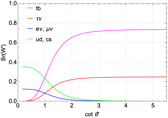
Figure 1: Main branching fractions as function of $\cot\theta^{\prime}$

As it is shown, for example in Ref. ZprimeToTTBarPaper , if the new particle was to have a non negligible decay width with respect to experimental resolutions, the sensitivity analysis to its existence could be reduced. In order to calculate the proton-proton production cross section, we make use of the MadGraph5_MC@NLO tool in the 5 flavor scheme Alwall:2014hca . The model Sullivan:2002jt ; Duffty:2012rf uses the Lagrangian as reported in Eq. (1) with the typical assumptions of the SSM: $g_{w}=e/\sin\theta_{W}$, $\alpha_{L}^{f_{i}f_{j}}=1$, $\alpha_{R}^{f_{i}f_{j}}=0$ and $V_{f_{i}f_{j}}=V_{\mathrm{CKM}}$. The third row and column of $V_{\mathrm{CKM}}^{SM}$ are approximated to (0,0,1). To simulate the Parton Density Functions (PDF) of protons, we use the NNPDF3.1Ball:2017nwa PDF set, derived at leading order and with $\alpha_{s}=0.118$. Table 2 reports the values of the cross section and their relative uncertainty for a centre-of-mass energy of $\sqrt{s}=13$ and 14 TeV. The values in Table 2 allow us to obtain the cross sections for the TF model by multiplying them times $\tan^{2}\theta^{\prime}$ since $h_{I,II}^{\prime}=g_{SM}\tan\theta^{\prime}$.

Mass	Width	Cross section (fb)
		13 TeV	14 TeV
1000	10	109552$\pm$407	127176$\pm$466
	100	10939$\pm$54	12674$\pm$ 59
	200	5355$\pm$21	6177 $\pm$ 23
1400	14	26036$\pm$123	31207$\pm$ 144
	140	2712$\pm$12	3246 $\pm$ 13
	280	1375$\pm$5	1633 $\pm$ 6
1800	18	7835$\pm$42	9717 $\pm$ 50
	180	859$\pm$4	1052 $\pm$ 5
	360	452$\pm$2	550 $\pm$ 3
2000	20	5375$\pm$29	5748 $\pm$ 30
	200	593$\pm$3	635 $\pm$ 3
	400	315$\pm$2	340 $\pm$ 2
2400	24	2005$\pm$11	2146 $\pm$ 13
	240	235$\pm$1	253 $\pm$ 1
	480	131,7$\pm$0,8	142,0$\pm$ 0,8
2800	28	791$\pm$4	850 $\pm$ 5
	280	102,4$\pm$0,7	110,4$\pm$ 0,7
	560	59,9$\pm$0,4	65,1 $\pm$ 0,4
3200	32	331$\pm$2	356 $\pm$ 2
	320	47,9$\pm$0,4	51,9 $\pm$ 0,4
	640	30,0$\pm$0,1	32,6 $\pm$ 0,1
3600	36	145$\pm$1	156 $\pm$ 1
	360	23,9$\pm$0,1	25,8 $\pm$ 0,1
	720	16,20$\pm$0,08	17,51$\pm$ 0,09
4000	40	67,3$\pm$0,6	71,8 $\pm$ 0,7
	400	13,10$\pm$0,06	14,12$\pm$ 0,07
	800	9,43$\pm$0,04	10,25$\pm$ 0,04
4400	44	34,1$\pm$0,1	35,7 $\pm$ 0,1
	440	7,61$\pm$0,04	8,20 $\pm$ 0,04
	880	5,76$\pm$0,02	6,24 $\pm$ 0,03
4800	48	18,18$\pm$0,03	18,91$\pm$ 0,03
	480	4,70$\pm$0,03	5,07 $\pm$ 0,03
	960	3,77$\pm$0,02	4,09 $\pm$ 0,02
5200	52	10,17$\pm$0,03	10,67$\pm$ 0,02
	520	3,06$\pm$0,02	3,34 $\pm$ 0,02
	1040	2,54$\pm$0,01	2,77 $\pm$ 0,02
5600	56	5,91$\pm$0,01	6,40 $\pm$ 0,01
	560	2,07$\pm$0,01	2,28 $\pm$ 0,01
	1120	1,798$\pm$0,007	1,958$\pm$ 0,007
6000	60	3,528$\pm$0,005	4,046$\pm$ 0,007
	600	1,49$\pm$0,01	1,63 $\pm$ 0,01
	1200	1,304$\pm$0,008	1,428$\pm$ 0,005

Table 2: Cross section values and their relative uncertainties obtained with the MadGraph5_MC@NLO generator for narrow (1%) and wide (10%, 20%, and 30%) widths $\text{W}^{\prime}$ boson for different mass hypotheses for both 13 and 14 TeV.

V Method and results

As discussed in the previous sections, the TF model considered in this work has five free parameters $u$, $v$, $g_{12}$, $g_{3}$ e $g_{0}$. The constraints in Eqs. (17) and (18) allow to reduce the number of free parameters to two: $u$ and $\theta^{\prime}$. We require the correction terms due to the TopFlavor model in Eq. (18) for $M_{W}$ and $M_{Z}$ to be within the experimental error, thus constraining the allowed values of $\theta^{\prime}$ as a function of $u$. We impose a further constraint on the model, by considering that the interactions with the gauge bosons of both $SU(2)$ groups can be perturbatively treated. To accomplish this, we require that $g_{12}^{2},g_{3}^{2}<4\pi$, obtaining:

$$0.18<\,\tan\theta^{\prime}\,<5.5.$$ (27)

In our analysis, we scan $10^{6}$ points in the parameter space $(u,\theta^{\prime})$, with $\theta^{\prime}$ satisfying Eq. (27) and $u>800\,\text{GeV}$. These conditions ensure that the mass of $\text{W}^{\prime}$ is larger than $1\,\text{TeV}$. For each point of the parameter space we obtain the observable $M_{\text{W}^{\prime}}$, $\Gamma_{\text{Tot}}$, $\text{Br}(\text{W}^{\prime}\to tb)$, $\text{Br}(\text{W}^{\prime}\to\tau\,\nu_{\tau})$ from Eqs (18, 25, 26). We checked the constraints presented in Refs. malkawi1996model ; malkawi1999new ; Lee:2010zzq and they do not appear to modify the results mentioned above in the parameter space we considered. In Fig. 2 we show all the possible $\Gamma_{\text{Tot}}/M_{\text{W}^{\prime}}$ as a function of $M_{\text{W}^{\prime}}$. The value of $\Gamma_{\text{Tot}}/M_{\text{W}^{\prime}}$ depends only on $\theta^{\prime}$, which is the reason why we also show the right vertical axis in terms of $\cos 2\theta^{\prime}$. The total width can be up to $40\%$ of the $\text{W}^{\prime}$ boson mass for $\sin\theta^{\prime}=0.18$. On the other hand, the minimum value of $\Gamma_{\text{Tot}}/M_{\text{W}^{\prime}}$ is obtained for $\theta^{\prime}=\pi/4$, since for this angle we recover the prediction of the SSM $h_{I,II}^{\prime}=h_{III}^{\prime}=g_{SM}$. We note that the total $\text{W}^{\prime}$ boson width, $\Gamma_{\text{Tot}}$, is approximately proportional to the $\text{W}^{\prime}$ boson mass.

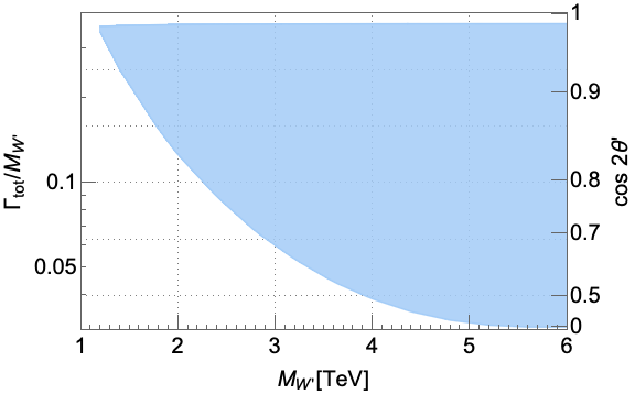
Figure 2: Allowed ranges for $\Gamma_{\text{Tot}}/M_{\text{W}^{\prime}}$ and $\cos\,2\theta^{\prime}$ for a fixed $M_{\text{W}^{\prime}}$ value.

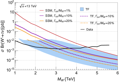
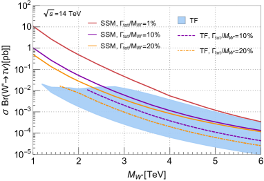
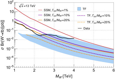
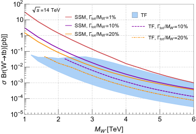
Figure 3: Theoretical predictions for $\sigma(pp\to\text{W}^{\prime})\text{Br}(\text{W}^{\prime}\to tb)$ (top panels) and $\sigma(pp\to\text{W}^{\prime})\text{Br}(\text{W}^{\prime}\to\tau\nu_{\tau})$ (bottom panels) as a function of $M_{\text{W}^{\prime}}$ at $\sqrt{s}=13\,\text{TeV}$ (left panels) and $\sqrt{s}=14\,\text{TeV}$ (right panels). The cyan band represents the allowed phase space from the TopFlavor prediction. The dashed violet and orange lines correspond to $\Gamma_{\text{Tot}}/M_{\text{W}^{\prime}}=0.1,\,0.2$ in the TF model respectively. The red, violet and orange continuous curves are the SSM predictions with $\alpha_{L}=1$, $\alpha_{R}=0$ for $\Gamma_{\text{Tot}}/M_{\text{W}^{\prime}}$ equal to 0.01,0.1, and 0.2 respectively. The black curve was built using the data in Ref.  Sirunyan:2017vkm ; Sirunyan_2019 .

In Fig. 3 we show the cross section times the branching fractions to the third family fermions:

$$\begin{split}&\sigma(pp\to\text{W}^{\prime})\text{Br}(\text{W}^{\prime}\to tb),\\ &\sigma(pp\to\text{W}^{\prime})\text{Br}(\text{W}^{\prime}\to\tau\nu_{\tau}),\end{split}$$ (28)

as a function of $M_{\text{W}^{\prime}}$ for a centre-of-mass energy of $\sqrt{s}=13$ and 14 TeV. The cyan band represents the parameter space allowed by the TF model. The red line stands for the SSM predicted cross section for $\Gamma_{\text{Tot}}=0.01\,M_{\text{W}^{\prime}}$. For comparison purposes, the predicted cross section for values of $\Gamma_{\text{Tot}}$ equal to $0.1\,M_{\text{W}^{\prime}}$, and $0.2\,M_{\text{W}^{\prime}}$ in both the SSM and TF assumptions are also shown. From these plots is possible to notice that the TF model is up to one order of magnitude smaller than the SSM.

The black lines represent the most recent exclusion limits obtained by the CMS Collaboration Sirunyan:2017vkm ; Sirunyan_2019 in the context of the W^′ boson searches in those two decay channels. Those plots showcase the portion of the phase space allowed in the TF model is still not excluded by direct searches. The top-left panel of Fig. 3 in particular shows that only values of the $\text{W}^{\prime}$ mass below 1.6 TeV are excluded in the $\tau\nu$ channels for any value of $\theta^{\prime}$. Larger values of the mass are possible, with a production cross section times branching fraction of order of magnitude 1 fb, i.e. below the data upper limit. For the $tb$ decay channel, the bottom-left panel shows that a large portion of the phase space is still available, as values of $M_{\text{W}^{\prime}}$ between 2.2 and 4 TeV are excluded only on for cross sections times branching ratio above order of 10 fb. It is also noteworthy that in the allowed region corresponds the total decay width $\Gamma_{\text{Tot}}$ can assume values up to 36% of the particle mass, which can result in differences in the observable quantities used in physics analyses.

The increase of the centre-of-mass energy at the LHC collider to 14 TeV would increase the production cross sections by a factor $1.1$.

Before conclusions we would like to comment on the recent measurement of the muon magnetic anomaly $g-2$ Abi:2021gix , exhibiting a discrepancy with the expected theoretical value at a significance level of $4.2$ standard deviations. From Ref. Biggio_2016 one can infer that new physics contributions to $\Delta a_{\mu}$ in the TF scheme are suppressed for masses of the order of TeV and above.

VI Conclusions

LHC searches for new physics also by looking for new charged $\text{W}^{\prime}$ gauge bosons through a variety of final states including leptons Sirunyan:2018mpc ; Sirunyan:2019vgj ; Sirunyan_2019 ; Sirunyan:2017vkm or quarks Atlas_wtolep ; Aaboud:2017yvp ; Aaboud:2018vgh ; Aaboud_2019 ; Aaboud:2018juj ; CMS:2021mux . Models based on the Sequential Standard Model are often used as benchmarks for such analyses that look after final states where the $\text{W}^{\prime}$ decays to fermions. Even if the SSM incorporates a wide variety of models, other theories predicting new heavy bosons might have realizations that are not allowed in the SSM, and that have not been yet excluded by data. We provide the particular case of the TopFlavor model, where a phenomenological study is performed, and the allowed parameter range is explored and expressed in terms of observable quantities at the LHC, like the new particle mass or width. For fixed values of $\Gamma_{\mathrm{tot}}/M_{\text{W}^{\prime}}$, the study resulted in:

$$10^{-1}\lesssim\frac{\left[\sigma(pp\to\text{W}^{\prime})\cdot\text{Br}(\text{W}^{\prime}\to ff)\right]_{\rm\text{TF}}}{\left[\sigma(pp\to\text{W}^{\prime})\cdot\text{Br}(\text{W}^{\prime}\to ff)\right]_{\rm\text{SSM}}}\lesssim 1\,.$$

This shows that a more systematic study of $\text{W}^{\prime}$-models for LHC search is required.

While standard CMS and ATLAS analyses have already performed thorough searches for a $\text{W}^{\prime}$ in the $tb$ and in $\tau\nu$ final states, in the TopFlavor model such measurements provide lower limits for the $M_{\text{W}^{\prime}}$ mass of the order of $2\,\text{TeV}$. A significant portion of the phase space is therefore still allowed in the TopFlavor model.

References

- [1] J. P. Lees et al. Evidence for an Excess of Decays. Phys. Rev. Lett., 109:101802, Sep 2012.
- [2] S. Hirose et al. Measurement of the Lepton Polarization and in the Decay . Phys. Rev. Lett., 118:211801, May 2017.
- [3] R. Aaij et al. Measurement of the Ratio of Branching Fractions . Phys. Rev. Lett., 115:111803, Sep 2015.
- [4] J. P. Lees et al. Measurement of branching fractions and rate asymmetries in the rare decays . Phys. Rev. D, 86:032012, Aug 2012.
- [5] S. Choudhury et al. Test of lepton flavor universality and search for lepton flavor violation in decays. JHEP, 03:105, 2021.
- [6] R. Aaij et al. Test of lepton universality in beauty-quark decays, 2021.
- [7] Gudrun Hiller and Ivan Nisandzic. and beyond the standard model. Phys. Rev. D, 96(3):035003, 2017.
- [8] G. W. Bennett, B. Bousquet, H. N. Brown, G. Bunce, R. M. Carey, P. Cushman, G. T. Danby, P. T. Debevec, M. Deile, H. Deng, and et al. Final report of the E821 muon anomalous magnetic moment measurement at BNL. Physical Review D, 73(7), Apr 2006.
- [9] B. Abi et al. Measurement of the Positive Muon Anomalous Magnetic Moment to 0.46 ppm. Phys. Rev. Lett., 126:141801, 2021.
- [10] Jogesh C Pati and Abdus Salam. Lepton number as the fourth “color”. In Selected Papers Of Abdus Salam: (With Commentary), pages 343–357. World Scientific, 1994.
- [11] N Mohapatra Rabindra. Unification and supersymmetry: The Frontiers of quark-lepton physics., volume 1. Springer, 1986.
- [12] Eric Corrigan. LEFT-RIGHT-SYMMETRIC MODEL BUILDING. Master’s thesis, Lund U., 2015.
- [13] F Pisano and Vicente Pleitez. SU(3)U(1) model for electroweak interactions. Physical Review D, 46(1):410, 1992.
- [14] Andrzej J Buras, Fulvia De Fazio, Jennifer Girrbach, and Maria V Carlucci. The anatomy of quark flavour observables in 331 models in the flavour precision era. Journal of High Energy Physics, 2013(2):23, 2013.
- [15] Sofiane M Boucenna, José WF Valle, and Avelino Vicente. Predicting charged lepton flavor violation from 3-3-1 gauge symmetry. Physical Review D, 92(5):053001, 2015.
- [16] JM Cabarcas, D Gomez Dumm, and R Martinez. Flavor-changing neutral currents in 331 models. Journal of Physics G: Nuclear and Particle Physics, 37(4):045001, 2010.
- [17] D Cogollo, FS Queiroz, PR Teles, and A Vital de Andrade. Novel sources of Flavor Changed Neutral Currents in the 331 RHN model. The European Physical Journal C, 72(5):2029, 2012.
- [18] Hock-Seng Goh and Christopher A Krenke. Little twin Higgs model. Physical Review D, 76(11):115018, 2007.
- [19] Martin Schmaltz. The simplest little Higgs. Journal of High Energy Physics, 2004(08):056, 2004.
- [20] Oleg Antipin, Matin Mojaza, and Francesco Sannino. Jumping out of the light-Higgs conformal window. Physical Review D, 87(9), May 2013.
- [21] Aqeel Ahmed. Heavy Higgs of the twin Higgs models. Journal of High Energy Physics, 2018(2):48, 2018.
- [22] Zackaria Chacko, Hock-Seng Goh, and Roni Harnik. A twin Higgs model from left-right symmetry. Journal of High Energy Physics, 2006(01):108, 2006.
- [23] Paul Langacker. The physics of heavy gauge bosons. Reviews of Modern Physics, 81(3):1199, 2009.
- [24] CMS Collaboration. Search for a W’ boson decaying to a bottom quark and a top quark in pp collisions at TeV, 2012.
- [25] Guido Altarelli, Barbara Mele, and M Ruiz-Altaba. Searching for new heavy vector bosons in p colliders. Zeitschrift für Physik C Particles and Fields, 45(1):109–121, 1989.
- [26] Xiao-yuan Li and Ernest Ma. Gauge model of generation non-universality re-examined. Journal of Physics G: Nuclear and Particle Physics, 19(9):1265, 1993.
- [27] Ehab Malkawi, Tim Tait, and C-P Yuan. A model of strong flavor dynamics for the top quark. Physics Letters B, 385(1-4):304–310, 1996.
- [28] Xiao-yuan Li and Ernest Ma. Gauge model of generation nonuniversality. Phys. Rev. Lett., 47:1788–1791, Dec 1981.
- [29] Jong Chul Lee, Kang Young Lee, and Jae Kwan Kim. Phenomenological implications of the topflavour model. Physics Letters B, 424(1-2):133–142, 1998.
- [30] David J Muller and Satyanarayan Nandi. Topflavor: a separate SU(2) for the third family. Physics Letters B, 383(3):345–350, Sep 1996.
- [31] Junjie Cao, Liangliang Shang, Wei Su, Fei Wang, and Yang Zhang. Interpreting the 750 GeV diphoton excess within topflavor seesaw model. Nuclear Physics B, 911:447–470, 2016.
- [32] David J Muller and Satya Nandi. A separate SU(2) for the third family: Topflavor. Nuclear Physics B-Proceedings Supplements, 52(1-2):192–194, 1997.
- [33] Ehab Malkawi, EI Lashin, and Hatem Widyan. Light sterile neutrino in the top-flavor model. Physical Review D, 62(3):033005, 2000.
- [34] http://pdg.lbl.gov/2019/tables/contents_tables.html.
- [35] Albert M Sirunyan et al. Search for high-mass resonances in final states with a lepton and missing transverse momentum at TeV. JHEP, 06:128, 2018.
- [36] Albert M Sirunyan et al. Search for high mass dijet resonances with a new background prediction method in proton-proton collisions at 13 TeV. JHEP, 05:033, 2020.
- [37] Albert M Sirunyan et al. Search for a W′ boson decaying to a lepton and a neutrino in proton-proton collisions at TeV. Physics Letters B, 792:107–131, May 2019.
- [38] Albert M Sirunyan et al. Search for heavy resonances decaying to a top quark and a bottom quark in the lepton+jets final state in proton-proton collisions at 13 TeV. Phys. Lett. B, 777:39–63, 2018.
- [39] Morad Aaboud et al. Search for a heavy charged boson in events with a charged lepton and missing transverse momentum from collisions at with the ATLAS detector. Phys. Rev. D, 100:052013, Sep 2019.
- [40] Morad Aaboud et al. Search for new phenomena in dijet events using 37 fb-1 of collision data collected at 13 TeV with the ATLAS detector. Phys. Rev. D, 96(5):052004, 2017.
- [41] Morad Aaboud et al. Search for High-Mass Resonances Decaying to in pp Collisions at =13 TeV with the ATLAS Detector. Phys. Rev. Lett., 120(16):161802, 2018.
- [42] M. Aaboud, G. Aad, B. Abbott, O. Abdinov, B. Abeloos, D.K. Abhayasinghe, S.H. Abidi, O.S. AbouZeid, N.L. Abraham, H. Abramowicz, and et al. Search for vector-boson resonances decaying to a top quark and bottom quark in the lepton plus jets final state in pp collisions at TeV with the ATLAS detector. Physics Letters B, 788:347–370, Jan 2019.
- [43] Morad Aaboud et al. Search for decays in the hadronic final state using pp collisions at TeV with the ATLAS detector. Phys. Lett. B, 781:327–348, 2018.
- [44] Albert M Sirunyan et al. Search for W’ bosons decaying to a top and a bottom quark at s=13TeV in the hadronic final state. Phys. Lett. B, 820:136535, 2021.
- [45] Yeong Gyun Kim and Kang Young Lee. Early LHC bound on the W′ boson mass in the non-universal gauge interaction model. Physics Letters B, 706(4):367–370, 2012.
- [46] Yeong Gyun Kim and Kang Young Lee. Direct search for heavy gauge bosons at the LHC in the non-universal SU(2) model. Phys. Rev. D, 90:117702, Dec 2014.
- [47] A. M. Sirunyan, A. Tumasyan, W. Adam, F. Ambrogi, E. Asilar, T. Bergauer, J. Brandstetter, M. Dragicevic, J. Erö, and et al. Search for resonant production in proton-proton collisions at TeV. Journal of High Energy Physics, 2019(4), Apr 2019.
- [48] J. Alwall, R. Frederix, S. Frixione, V. Hirschi, F. Maltoni, O. Mattelaer, H. S. Shao, T. Stelzer, P. Torrielli, and M. Zaro. The automated computation of tree-level and next-to-leading order differential cross sections, and their matching to parton shower simulations. JHEP, 07:079, 2014.
- [49] Zack Sullivan. Fully Differential Production and Decay at Next-to-Leading Order in QCD. Phys. Rev. D, 66:075011, 2002.
- [50] Daniel Duffty and Zack Sullivan. Model independent reach for W-prime bosons at the LHC. Phys. Rev. D, 86:075018, 2012.
- [51] Richard D. Ball et al. Parton distributions from high-precision collider data. Eur. Phys. J. C, 77(10):663, 2017.
- [52] Ehab Malkawi and C-P Yuan. New physics in the third family and its effect on low-energy data. Physical Review D, 61(1):015007, 1999.
- [53] Kang Young Lee. Lepton flavour violation in a nonuniversal gauge interaction model. Phys. Rev. D, 82:097701, 2010.
- [54] Sz Borsanyi, Z Fodor, JN Guenther, C Hoelbling, SD Katz, L Lellouch, T Lippert, K Miura, L Szabo, F Stokes, et al. Leading-order hadronic vacuum polarization contribution to the muon magnetic momentfrom lattice QCD. arXiv preprint arXiv:2002.12347, 2020.
- [55] Carla Biggio, Marzia Bordone, Luca Di Luzio, and Giovanni Ridolfi. Massive vectors and loop observables: the g-2 case. Journal of High Energy Physics, 2016(10), Oct 2016.