Improving Optimal Power Flow Relaxations Using 3-Cycle Second-Order Cone Constraints

Abstract

This paper develops a novel second order cone relaxation of the semidefinite programming formulation of optimal power flow, that does not imply the ‘angle relaxation’. We build on a technique developed by Kim et al., extend it for complex matrices, and apply it to $3\times 3$ positive semidefinite matrices to generate novel second-order cone constraints that augment upon the well-known $2\times 2$ principal-minor based second-order cone constraints. Finally, we apply it to optimal power flow in meshed networks and provide numerical illustrations.

I Introduction and Background

Convex relaxation of nonlinear optimization models has been successfully applied to optimal power flow in the context of certifying global optimality or infeasibility [1], as well as in enabling mixed-integer nonlinear optimization. The tightest known relaxations are based on semidefinite programming (SDP) forms, either by construction, or generated as part of the Lasserre hierarchy [2]. Since the scalability of SDP is limited in practice, so there remains a need for tight but scalable relaxations. Second-order cone (SOC) programming is considered more scalable, and mixed-integer (MI) SOC solvers are commercially available.

It is noted that the physical interpretation of the difference between the SDP and the SOC relaxation is the ‘angle relaxation’ [3], that is, Kirchhoff’s voltage law in loops is not represented beyond the implications of Ohm’s law on voltage magnitude. Therefore, Kocuk et al. developed valid inequalities to include the physics of 3 and 4-cycles in a SOC formulation [4], by iteratively adding linear inequalities based on 3 and 4-cycle SDP subproblems. Alternatively, Coffrin et al. intersect the conventional SDP/SOC BIM power/lifted-voltage formulation with a convex hull power/polar-voltage formulation [5], which therefore also improves upon the angle-related physics representation. Hijazi et al. [6] develop polynomial expressions for $3\times 3$ minors and propose an interpretation w.r.t. Kirchhoff’s voltage law.

Alternatively, in this paper, we propose a method to generate tighter SOC relaxations, based on a technique of Kim et al. [7], and apply it to SDP optimization models for meshed power networks. It will be shown that the novel SOC formulation improves upon the conventional, $2\times 2$ principal minor based SOC relaxation (abbreviated PM SOC here) of the bus injection model (BIM) optimal power flow (OPF) formulation [3]. Finally, we provide an intuitive interpretation of the novel SOC constraints for 3-cycles by comparing the expressions with those published by Hijazi et al. [6] and Kocuk et al. [8].

II Kim et al. SDP to SOC Relaxation

Kim et al. [7] develop a SDP to SOC relaxation procedure in the real numbers, whereas this section develops the generalization to complex matrices; staying in the complex domain enables tighter relaxations. Specifically, we adapt the derivation §3 ‘An extension of the SOC relaxation of type 1’, Lemma 3.2 [7] to Hermitian matrices (a.k.a. complex symmetric).

We partition an Hermitian, positive semidefinite (PSD) variable matrix ${\color[rgb]{0,0,1}\mathbf{M}}$ as,

$${\color[rgb]{0,0,1}\mathbf{M}}=\begin{bmatrix}{\color[rgb]{0,0,0}\alpha}&{\color[rgb]{0,0,1}\mathbf{a}}^{\text{H}}\\ {\color[rgb]{0,0,1}\mathbf{a}}&{\color[rgb]{0,0,1}\mathbf{A}}\\ \end{bmatrix}\succeq 0.$$ (1)

where superscript H is the conjugate transpose. Note that in general we could position the scalar $\alpha$ anywhere on the diagonal through a permutation of the rows and columns. This results in the following matrix variable sizes and structures:

$${\color[rgb]{0,0,1}\mathbf{M}}\in{\color[rgb]{.25,.25,.25}\mathbb{H}^{n+1}},{\color[rgb]{0,0,1}\mathbf{A}}=\mathbf{A}^{\text{re}}+{\color[rgb]{1,0,0}j}\mathbf{A}^{\text{im}}\in{\color[rgb]{.25,.25,.25}\mathbb{H}^{n}},{\color[rgb]{.25,.25,.25}\mathbb{S}_{+}^{n}},$$

$${\color[rgb]{0,0,1}\mathbf{a}}=\mathbf{a}^{\text{re}}+{\color[rgb]{1,0,0}j}\mathbf{a}^{\text{im}}\in{\color[rgb]{.25,.25,.25}\mathbb{C}^{n\times 1}},{\color[rgb]{0,0,0}\alpha}\in{\color[rgb]{.25,.25,.25}\mathbb{R}^{1\times 1}},{\color[rgb]{0,0,0}\alpha}\geq 0.$$

We choose a complex matrix parameter ${\color[rgb]{.75,.5,.25}\mathbf{c}}$ and derive ${\color[rgb]{.75,.5,.25}\mathbf{C}}$,

$${\color[rgb]{.75,.5,.25}\mathbf{c}}={\color[rgb]{1,0,0}\mathbf{c}}^{\text{re}}+{\color[rgb]{1,0,0}j}{\color[rgb]{1,0,0}\mathbf{c}}^{\text{im}}\in{\color[rgb]{.25,.25,.25}\mathbb{C}^{n\times q}},\quad{\color[rgb]{.75,.5,.25}\mathbf{C}}={\color[rgb]{1,0,0}\mathbf{C}}^{\text{re}}+{\color[rgb]{1,0,0}j}{\color[rgb]{1,0,0}\mathbf{C}}^{\text{im}}={\color[rgb]{.75,.5,.25}\mathbf{c}}{\color[rgb]{.75,.5,.25}\mathbf{c}}^{\text{H}},$$

or vice-versa we choose ${\color[rgb]{.75,.5,.25}\mathbf{C}}\in{\color[rgb]{.25,.25,.25}\mathbb{H}^{n}},{\color[rgb]{.25,.25,.25}\mathbb{S}_{+}^{n}}$ and factor it into ${\color[rgb]{.75,.5,.25}\mathbf{c}}$. We use $\bullet$ to represent the Frobenius inner product of two matrices,

$${\color[rgb]{.75,.5,.25}\mathbf{C}}\bullet{\color[rgb]{0,0,1}\mathbf{A}}=\sum_{ij}([{\color[rgb]{.75,.5,.25}\mathbf{C}}]_{ij})^{*}[{\color[rgb]{0,0,1}\mathbf{A}}]_{ij},$$ (2)

where $[\mathbf{X}]_{ij}$ means extracting the scalar at index $(i,j)$ in matrix $\mathbf{X}$, and superscript $*$ is the complex conjugate. For PSD Hermitian matrices this product is nonnegative,

$${\color[rgb]{.75,.5,.25}\mathbf{C}}\bullet{\color[rgb]{0,0,1}\mathbf{A}}\geq 0.$$ (3)

We now illustrate Kim et al.’s main result, a valid convex quadratic inequality for a sampled ${\color[rgb]{.75,.5,.25}\mathbf{C}}={\color[rgb]{.75,.5,.25}\mathbf{c}}{\color[rgb]{.75,.5,.25}\mathbf{c}}^{\text{H}}$, for any Hermitian and PSD matrix ${\color[rgb]{0,0,1}\mathbf{M}}$ partitioned with a scalar $\alpha$ on the diagonal:

$$({\color[rgb]{.75,.5,.25}\mathbf{c}}^{\text{H}}{\color[rgb]{0,0,1}\mathbf{a}})^{\text{H}}({\color[rgb]{.75,.5,.25}\mathbf{c}}^{\text{H}}{\color[rgb]{0,0,1}\mathbf{a}})\leq{\color[rgb]{0,0,0}\alpha}\cdot({\color[rgb]{.75,.5,.25}\mathbf{C}}\bullet{\color[rgb]{0,0,1}\mathbf{A}}).$$ (4)

Implementation can use identities w.r.t. the reals,

$${\color[rgb]{.75,.5,.25}\mathbf{C}}\bullet{\color[rgb]{0,0,1}\mathbf{A}}=\mathbf{C}^{\text{re}}\bullet\mathbf{A}^{\text{re}}+\mathbf{C}^{\text{im}}\bullet\mathbf{A}^{\text{im}},$$

$$\operatorname{Re}({\color[rgb]{.75,.5,.25}\mathbf{c}}^{\text{H}}{\color[rgb]{0,0,1}\mathbf{a}})=({\color[rgb]{1,0,0}\mathbf{c}}^{\text{re}})^{\text{T}}\mathbf{a}^{\text{re}}+({\color[rgb]{1,0,0}\mathbf{c}}^{\text{im}})^{\text{T}}\mathbf{a}^{\text{im}},$$

$$\operatorname{Im}({\color[rgb]{.75,.5,.25}\mathbf{c}}^{\text{H}}{\color[rgb]{0,0,1}\mathbf{a}})=({\color[rgb]{1,0,0}\mathbf{c}}^{\text{re}})^{\text{T}}\mathbf{a}^{\text{im}}-({\color[rgb]{1,0,0}\mathbf{c}}^{\text{im}})^{\text{T}}\mathbf{a}^{\text{re}}.$$

Note that we directly derive (real-value) SOCs for complex-value PSD constraints, without having to invoke the isomorphism between the complex numbers and $2\times 2$ matrices (in its block matrix form) on ${\color[rgb]{0,0,1}\mathbf{A}}$ or ${\color[rgb]{0,0,1}\mathbf{M}}$.

III Application to a $3\times 3$ PSD Voltage Matrix

We focus on a 3-bus fully connected power network in this section, and discuss generalization later. Using the BIM OPF [3] model for a 3-bus system, with bus voltages ${\color[rgb]{0,0,1}U_{i}}=U^{\text{re}}_{i}+{\color[rgb]{1,0,0}j}U^{\text{im}}_{i}$, the system ‘${\color[rgb]{0,0,1}\mathbf{M}}$’ matrix in the ‘W’ variable space corresponds to:

$$\begin{bmatrix}U^{\text{re}}_{1}+{\color[rgb]{1,0,0}j}U^{\text{im}}_{1}\\ U^{\text{re}}_{2}+{\color[rgb]{1,0,0}j}U^{\text{im}}_{2}\\ U^{\text{re}}_{3}+{\color[rgb]{1,0,0}j}U^{\text{im}}_{3}\\ \end{bmatrix}\begin{bmatrix}U^{\text{re}}_{1}+{\color[rgb]{1,0,0}j}U^{\text{im}}_{1}\\ U^{\text{re}}_{2}+{\color[rgb]{1,0,0}j}U^{\text{im}}_{2}\\ U^{\text{re}}_{3}+{\color[rgb]{1,0,0}j}U^{\text{im}}_{3}\\ \end{bmatrix}^{\text{H}}$$ (5)

$$=\begin{bmatrix}W^{\text{re}}_{11}&W^{\text{re}}_{12}+{\color[rgb]{1,0,0}j}W^{\text{im}}_{12}&W^{\text{re}}_{13}+{\color[rgb]{1,0,0}j}W^{\text{im}}_{13}\\ W^{\text{re}}_{12}-{\color[rgb]{1,0,0}j}W^{\text{im}}_{12}&W^{\text{re}}_{22}&W^{\text{re}}_{23}+{\color[rgb]{1,0,0}j}W^{\text{im}}_{23}\\ W^{\text{re}}_{13}-{\color[rgb]{1,0,0}j}W^{\text{im}}_{13}&W^{\text{re}}_{23}-{\color[rgb]{1,0,0}j}W^{\text{im}}_{23}&W^{\text{re}}_{33}\\ \end{bmatrix}={\color[rgb]{0,0,1}\mathbf{M}}\succeq 0$$

The partitions (1) then are,

$${\color[rgb]{0,0,1}\mathbf{A}}\!:\!\begin{bmatrix}W^{\text{re}}_{22}\!\!&\!\!W^{\text{re}}_{23}\!+\!{\color[rgb]{1,0,0}j}W^{\text{im}}_{23}\\ W^{\text{re}}_{23}\!-\!{\color[rgb]{1,0,0}j}W^{\text{im}}_{23}\!\!&\!\!W^{\text{re}}_{33}\\ \end{bmatrix},{\color[rgb]{0,0,1}\mathbf{a}}\!:\!\begin{bmatrix}W^{\text{re}}_{12}\!-\!{\color[rgb]{1,0,0}j}W^{\text{im}}_{12}\\ W^{\text{re}}_{13}\!-\!{\color[rgb]{1,0,0}j}W^{\text{im}}_{13}\end{bmatrix},\alpha\!:\!W^{\text{re}}_{11}.$$

III-A $2\times 2$ Principal Minor SOC Constraints

For this partition, substituting ${\color[rgb]{.75,.5,.25}\mathbf{c}}=\begin{bmatrix}1&0\end{bmatrix}^{\text{T}}$ or $\begin{bmatrix}0&1\end{bmatrix}^{\text{T}}$ into (4) generates known $2\times 2$ PM SOCs, i.e.

$$(W^{\text{re}}_{12})^{2}+(W^{\text{im}}_{12})^{2}\leq W^{\text{re}}_{11}W^{\text{re}}_{22}.$$ (6)

$$(W^{\text{re}}_{13})^{2}+(W^{\text{im}}_{13})^{2}\leq W^{\text{re}}_{11}W^{\text{re}}_{33},$$ (7a)

A partition with $\alpha=W^{\text{re}}_{22}$ or $\alpha=W^{\text{re}}_{33}$ and a one-hot ${\color[rgb]{.75,.5,.25}\mathbf{c}}$ generates the third unique PM SOC, i.e.,

$$(W^{\text{re}}_{23})^{2}+(W^{\text{im}}_{23})^{2}\leq W^{\text{re}}_{22}W^{\text{re}}_{33}.$$ (8a)

III-B Kim et al. SOC Constraints

We sample from the space of vectors ${\color[rgb]{.75,.5,.25}\mathbf{c}}\in{\color[rgb]{.25,.25,.25}\mathbb{C}^{2\times 1}}$ with the first element normalized, and parameterize through ${\color[rgb]{1,0,0}r},{\color[rgb]{1,0,0}\theta}$,

$${\color[rgb]{.75,.5,.25}\mathbf{c}}=\begin{bmatrix}1\\ {\color[rgb]{1,0,0}r}e^{{\color[rgb]{1,0,0}j}{\color[rgb]{1,0,0}\theta}}\end{bmatrix}=\begin{bmatrix}1\\ {\color[rgb]{1,0,0}r}\cos({\color[rgb]{1,0,0}\theta})\end{bmatrix}+{\color[rgb]{1,0,0}j}\begin{bmatrix}0\\ {\color[rgb]{1,0,0}r}\sin({\color[rgb]{1,0,0}\theta})\end{bmatrix},$$

Next we obtain a parameterized family of valid SOCs:

$$(W^{\text{re}}_{12}+{\color[rgb]{1,0,0}r}\cos({\color[rgb]{1,0,0}\theta})W^{\text{re}}_{13}-{\color[rgb]{1,0,0}r}\sin({\color[rgb]{1,0,0}\theta})W^{\text{im}}_{13})^{2}$$

$$+(W^{\text{im}}_{12}+{\color[rgb]{1,0,0}r}\cos({\color[rgb]{1,0,0}\theta})W^{\text{im}}_{13}+{\color[rgb]{1,0,0}r}\sin({\color[rgb]{1,0,0}\theta})W^{\text{re}}_{13})^{2}$$

$$\!\!\leq W^{\text{re}}_{11}\left(W^{\text{re}}_{22}+{\color[rgb]{1,0,0}r}^{2}W^{\text{re}}_{33}+2{\color[rgb]{1,0,0}r}\!\left(\cos({\color[rgb]{1,0,0}\theta})W^{\text{re}}_{23}-\sin({\color[rgb]{1,0,0}\theta})W^{\text{im}}_{23}\right)\right)\!.$$ (9)

We also generate them for the other partitions, i.e.,

$$(W^{\text{re}}_{12}+{\color[rgb]{1,0,0}r}\cos({\color[rgb]{1,0,0}\theta})W^{\text{re}}_{23}-{\color[rgb]{1,0,0}r}\sin({\color[rgb]{1,0,0}\theta})W^{\text{im}}_{23})^{2}$$

$$+(W^{\text{im}}_{12}-{\color[rgb]{1,0,0}r}\cos({\color[rgb]{1,0,0}\theta})W^{\text{im}}_{23}-{\color[rgb]{1,0,0}r}\sin({\color[rgb]{1,0,0}\theta})W^{\text{re}}_{23})^{2}$$

$$\!\!\leq W^{\text{re}}_{22}\left(W^{\text{re}}_{11}+{\color[rgb]{1,0,0}r}^{2}W^{\text{re}}_{33}+2{\color[rgb]{1,0,0}r}\!\left(\cos({\color[rgb]{1,0,0}\theta})W^{\text{re}}_{13}-\sin({\color[rgb]{1,0,0}\theta})W^{\text{im}}_{13}\right)\right)\!.$$ (10)

$$(W^{\text{re}}_{13}+{\color[rgb]{1,0,0}r}\cos({\color[rgb]{1,0,0}\theta})W^{\text{re}}_{23}+{\color[rgb]{1,0,0}r}\sin({\color[rgb]{1,0,0}\theta})W^{\text{im}}_{23})^{2}$$

$$+(W^{\text{im}}_{13}+{\color[rgb]{1,0,0}r}\cos({\color[rgb]{1,0,0}\theta})W^{\text{im}}_{23}-{\color[rgb]{1,0,0}r}\sin({\color[rgb]{1,0,0}\theta})W^{\text{re}}_{23})^{2}$$

$$\!\!\!\!\leq W^{\text{re}}_{33}\!\left(W^{\text{re}}_{11}+{\color[rgb]{1,0,0}r}^{2}W^{\text{re}}_{22}+2{\color[rgb]{1,0,0}r}\!\left(\cos({\color[rgb]{1,0,0}\theta})W^{\text{re}}_{12}-\sin({\color[rgb]{1,0,0}\theta})W^{\text{im}}_{12}\right)\right)\!.$$ (11)

Finally, we still need to state the linear inequalities based on the Frobenius inner product (3), i.e.,

$$W^{\text{re}}_{22}+{\color[rgb]{1,0,0}r^{2}}W^{\text{re}}_{33}+2{\color[rgb]{1,0,0}r}\left(\cos({\color[rgb]{1,0,0}\theta})W^{\text{re}}_{23}-\sin({\color[rgb]{1,0,0}\theta})W^{\text{im}}_{23}\right)\geq 0,$$ (12a)

$$W^{\text{re}}_{11}+{\color[rgb]{1,0,0}r^{2}}W^{\text{re}}_{33}+2{\color[rgb]{1,0,0}r}\left(\cos({\color[rgb]{1,0,0}\theta})W^{\text{re}}_{13}-\sin({\color[rgb]{1,0,0}\theta})W^{\text{im}}_{13}\right)\geq 0,$$ (13a)

$$W^{\text{re}}_{11}+{\color[rgb]{1,0,0}r^{2}}W^{\text{re}}_{22}+2{\color[rgb]{1,0,0}r}\left(\cos({\color[rgb]{1,0,0}\theta})W^{\text{re}}_{12}-\sin({\color[rgb]{1,0,0}\theta})W^{\text{im}}_{12}\right)\geq 0.$$ (14a)

Inequalities (9)-(11) are families of SOC constraints. One re-obtains a PM SOC for ${\color[rgb]{1,0,0}r}=0$, and similarly if one scales the second element of ${\color[rgb]{.75,.5,.25}\mathbf{c}}$ instead.

IV Interpretation with Kirchhoff’s Voltage Law

IV-A Kirchhoff’s Voltage Law for 3-Cycle in Lifted Voltage

Hijazi et al. [6] show that Kirchhoff’s voltage law (KVL) for a 3-cycle in the lifted voltage variable space is,

$$(W^{\text{re}}_{13}+{\color[rgb]{1,0,0}j}W^{\text{im}}_{13})^{*}(W^{\text{re}}_{23}+{\color[rgb]{1,0,0}j}W^{\text{im}}_{23})={W^{\text{re}}_{33}}(W^{\text{re}}_{12}+{\color[rgb]{1,0,0}j}W^{\text{im}}_{12})^{*}.$$ (15)

We note that this corresponds to a minor that involves only a single diagonal element, i.e. ‘type 2’ in [8]. In the reals, this becomes,

$$W^{\text{re}}_{13}W^{\text{re}}_{23}+W^{\text{im}}_{13}W^{\text{im}}_{23}=W^{\text{re}}_{33}W^{\text{re}}_{12},$$ (16a)

$$W^{\text{re}}_{13}W^{\text{im}}_{23}-W^{\text{im}}_{13}W^{\text{re}}_{23}=-W^{\text{re}}_{33}W^{\text{im}}_{12}.$$ (17a)

The real-value permuted 3-cycle KVL expressions are,

$$W^{\text{re}}_{12}W^{\text{re}}_{13}-W^{\text{im}}_{12}W^{\text{im}}_{13}=W^{\text{re}}_{11}W^{\text{im}}_{23},$$ (18a)

$$W^{\text{re}}_{12}W^{\text{im}}_{13}+W^{\text{im}}_{12}W^{\text{re}}_{13}=W^{\text{re}}_{11}W^{\text{im}}_{23},$$ (19a)

$$W^{\text{re}}_{12}W^{\text{re}}_{23}+W^{\text{im}}_{12}W^{\text{im}}_{23}=W^{\text{re}}_{22}W^{\text{re}}_{13},$$ (20a)

$$W^{\text{re}}_{12}W^{\text{im}}_{23}+W^{\text{im}}_{12}W^{\text{re}}_{23}=-W^{\text{re}}_{22}W^{\text{im}}_{13}.$$ (21a)

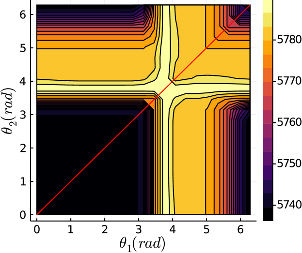
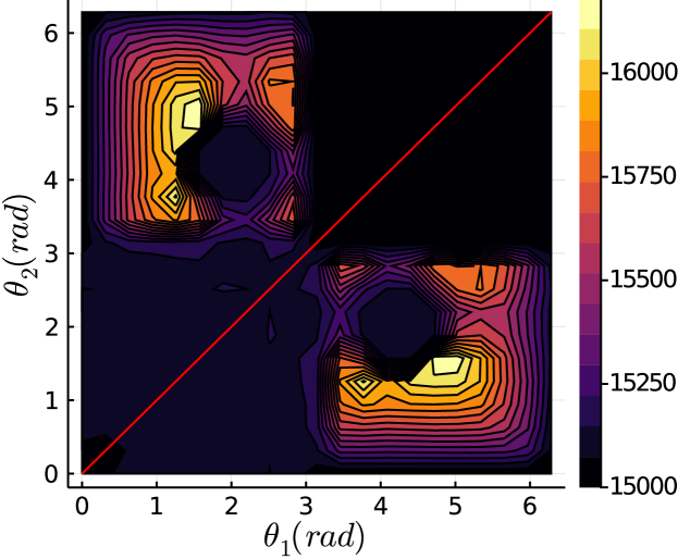
Figure 1: Contour plot for ‘case3_lmbd’

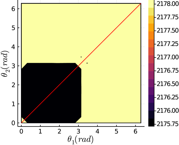
Figure 2: Contour plot for ‘case5_pjm’

Figure 3: Contour plot for ‘case14_ieee’

IV-B Kim et al. SOCs with Solution in Equality

If $\operatorname{rank}({\color[rgb]{0,0,1}\mathbf{M}})=1$, PM SOCs (7a)-(8a) are active,

$$(W^{\text{re}}_{13})^{2}+(W^{\text{im}}_{13})^{2}=W^{\text{re}}_{33}W^{\text{re}}_{11},$$ (22a)

$$(W^{\text{re}}_{23})^{2}+(W^{\text{im}}_{23})^{2}=W^{\text{re}}_{33}W^{\text{re}}_{22}.$$ (23a)

Under the same conditions, substituting ${\color[rgb]{1,0,0}r_{1}}={\color[rgb]{1,0,0}r_{2}}=1,$ and ${\color[rgb]{1,0,0}\theta_{1}}=0,{\color[rgb]{1,0,0}\theta_{2}}=\pi/2$, in (9) we obtain,

$$(W^{\text{re}}_{13}+W^{\text{re}}_{23})^{2}+(W^{\text{im}}_{13}+W^{\text{im}}_{23})^{2}$$

$$=W^{\text{re}}_{33}(W^{\text{re}}_{11}+W^{\text{re}}_{22}+2W^{\text{re}}_{12}),$$ (24a)

$$(W^{\text{re}}_{13}+W^{\text{im}}_{23})^{2}+(W^{\text{im}}_{13}-W^{\text{re}}_{23})^{2}$$

$$=W^{\text{re}}_{33}(W^{\text{re}}_{11}+W^{\text{re}}_{22}-2W^{\text{im}}_{12}).$$ (25a)

Therefore the following identities hold when $\operatorname{rank}({\color[rgb]{0,0,1}\mathbf{M}})=1$,

$$\eqref{eq_pm_ccaa}+\eqref{eq_pm_ccbb}+2\cdot\eqref{eq_cycle_c_real}\equiv\eqref{eq_kk_re_cc},$$

$$\eqref{eq_pm_ccaa}+\eqref{eq_pm_ccbb}+2\cdot\eqref{eq_cycle_c_imag}\equiv\eqref{eq_kk_im_cc},$$

as well as the equivalents for (18a)-(21a) (i.e. a total of 6 SOCs). This establishes that the Kim et al. SOCs include a stronger representation of KVL than just the PM SOCs. Note that this completing the square approach actually embeds nonconvex equalities (16a)-(21a) into a convex quadratic form.

Note that by themselves, (24a)-(25a) do not prove (16a)-(17a) hold; (22a)-(23a) are needed. Therefore observing that (9)-(11) are active in the solution is insufficient to prove that $\operatorname{rank}({\color[rgb]{0,0,1}\mathbf{M}})=1$. The PM SOCs (22a)-(23a) must also be active in the solution to give that confidence.

V Numerical Illustration

We extend the BIM implementation in PowerModels [9] and use 3-cycle PGLib test cases [10] with two ${\color[rgb]{1,0,0}\theta}$-parameterized SOCs per 3-cycle permutation. We use Ipopt [11] as the solver for NLP ‘AC’ OPF; Hypatia [12] for the BIM SDP and the Kim et al. SOC forms, and again Ipopt for the PM SOC. Fig. 3 - Fig. 3 show sweeps for two SOC families ${\color[rgb]{1,0,0}\theta_{1}},{\color[rgb]{1,0,0}\theta_{2}}$, w.r.t. objective value, for the 3, 5 and 14 bus test cases. The optimal ${\color[rgb]{1,0,0}\theta}$ for the 3-bus case is around $3.7$, with an objective value of $5790$. For ‘case5_pjm’, we want two distinct angles, i.e. ${\color[rgb]{1,0,0}\theta_{1}}\approx 1.6,{\color[rgb]{1,0,0}\theta_{2}}\approx 4.9$ with an objective of $16181$; for ‘case14_ieee’, one suffices, i.e. any ${\color[rgb]{1,0,0}\theta}\in[\pi;2\pi]$ gives objective $2178$. It is interesting that, to obtain the tightest relaxation, one case requires two fine-tuned angles, another requires one fine-tuned angle, and the third only requires one angle in a broader range. A condition for recognizing that a single angle is sufficient is that the maximum is on the diagonal of the plot. Table I summarizes numerical results in comparison with the NLP, SDP and PM SOC relaxations.

TABLE I: Objective values; Kim et al. SOCs for ${\color[rgb]{1,0,0}\theta_{1}}=0,{\color[rgb]{1,0,0}\theta_{2}}=3\pi/2$.

	AC NLP	BIM SDP	Kim+PM SOC	PM SOC
	$/h	% gap	% gap	% gap
case3_lmbd	5812.64	0.38	0.54	1.32
case5_pjm	17551.89	5.22	14.47	14.54
case14_ieee	2178.08	0.00	0.00	0.11

We note that in general, for the convergence of the interior point method to be strong, you want to avoid having a large amount of inequalities active in the solution. In general we expect this to be the case as many OPF problems are naturally low-rank [13]. Therefore, it may be beneficial to use the Kim et al. SOCs algorithmically as nonlinear cuts.

VI Conclusions

We develop a SOC relaxation does not entail the ‘angle relaxation’. For a $3\times 3$ Hermitian matrix, the Kim et al. SOCs sampled in two directions each ($2\times 3$ unique ones), when combined with the $2\times 2$ principal minor-derived SOCs (3 unique ones), clearly offers an tighter SOC relaxation. Combining with results by Hijazi et al. [6], we know now that when all 9 SOCs are satisfied in equality, it furthermore certifies that the original matrix is PSD and rank-1, and that the power flow satisfies Kirchhoff’s voltage law in a 3-cycle.

Nevertheless, these additional 6 SOCs may not be sufficient to obtain a relaxation that is equivalent to the SDP relaxation, as there are actually families of parameteric SOCs from which one needs to sample. The results do not suggest an obvious sampling strategy. Profiling on benchmark libraries [10] can aid in strategy development.

Real transmissions networks have loops in the topology that go beyond 3-cycles. Nevertheless, using chordal completion similar to [4], [14], we can re-cast the network graph in terms of intersected 3-cycles, and can apply the technique as such. It would be interesting to combine the Kim et al. SOCs with the QC formulation [5], to obtain a more scalable form than QC+SDP, and more accurate than QC+PM SOC. In future work, we plan to explore generating relaxations to $4\times 4$ and higher-dimensional PSD variable matrices directly. A prime use case is unbalanced SDP BIM OPF, as it relies on a large amount of $6\times 6$ complex PSD matrices, and solvers struggle with scalability and numerical stability [15].

References

• [1] S. Gopinath, H. L. Hijazi, T. Weisser, H. Nagarajan, M. Yetkin, K. Sundar, and R. W. Bent, “Proving global optimality of ACOPF solutions,” Electric Power Syst. Res., vol. 189, no. October 2019, p. 106688, 2020.
• [2] C. Josz and D. K. Molzahn, “Lasserre hierarchy for large scale polynomial optimization in real and complex variables,” SIAM Journal on Optimization, vol. 28, no. 2, pp. 1017–1048, 2018.
• [3] S. H. Low, “Convex relaxation of optimal power flow - part I: formulations and equivalence,” IEEE Trans. Control Netw. Syst., vol. 1, no. 1, pp. 15–27, mar 2014.
• [4] B. Kocuk, S. Dey, and S. Andy, “Strong SOCP relaxations of optimal power flow,” Operations Res., vol. 64, no. 6, pp. 1177–1196, apr 2016.
• [5] C. Coffrin, H. Hijazi, and P. Van Hentenryck, “The QC relaxation: a theoretical and computational study on optimal power flow,” IEEE Trans. Power Syst., vol. 31, no. 4, pp. 3008–3018, 2016.
• [6] H. Hijazi, C. Coffrin, and P. Van Hentenryck, “Polynomial SDP cuts for optimal power flow,” in PSCC, Genoa, Italy, 2016.
• [7] S. Kim, M. Kojima, and M. Yamashita, “Second order cone programming relaxation of a positive semidefinite constraint,” Optimization Methods Software, vol. 18, no. 5, pp. 535–541, 2003.
• [8] B. Kocuk, S. S. Dey, and X. A. Sun, “Matrix minor reformulation and SOCP-based spatial branch-and-cut method for the AC optimal power flow problem,” 2017. [Online]. Available: https://arxiv.org/pdf/1703.03050.pdf
• [9] C. Coffrin, R. Bent, K. Sundar, Y. Ng, and M. Lubin, “PowerModels.jl: an open-source framework for exploring power flow formulations,” in Power Syst. Comp. Conf., vol. 20, Dublin, Ireland, 2018, p. 8.
• [10] S. Babaeinejadsarookolaee, A. Birchfield, R. D. Christie, C. Coffrin, C. DeMarco, R. Diao, M. Ferris, S. Fliscounakis, S. Greene, R. Huang, C. Josz, R. Korab, B. Lesieutre, J. Maeght, D. K. Molzahn, T. J. Overbye, P. Panciatici, B. Park, J. Snodgrass, and R. Zimmerman, “The power grid library for benchmarking AC optimal power flow algorithms,” [math.OC], pp. 1–17, 2019.
• [11] A. Wächter and L. T. Biegler, “On the implementation of primal-dual interior point filter line search algorithm for large-scale nonlinear programming,” Math. Prog., vol. 106, no. 1, pp. 25–57, 2006.
• [12] C. Coey, L. Kapelevich, and J. P. Vielma, “Towards practical generic conic optimization,” pp. 1–25, 2020. [Online]. Available: http://arxiv.org/abs/2005.01136
• [13] J. Lavaei and S. H. Low, “Zero duality gap in optimal power flow problem,” IEEE Trans. Power Syst., vol. 27, no. 1, pp. 92–107, 2012.
• [14] R. A. Jabr, “Exploiting sparsity in SDP relaxations to the OPF problem,” IEEE Trans. Power Syst., vol. 27, no. 2, pp. 1138–1139, 2012.
• [15] L. Gan and S. H. Low, “Convex relaxations and linear approximation for optimal power flow in multiphase radial networks,” in Power Syst. Comp. Conf., Wroclaw, Poland, 2014, pp. 1–9.