The momentum distribution of two bosons in one dimension with infinite contact repulsion in harmonic trap gets analytical

Abstract

For a harmonically trapped system consisting of two bosons in one spatial dimension with infinite contact repulsion (hard core bosons), we derive an expression for the one-body density matrix $\rho_{B}$ in terms of centre of mass and relative coordinates of the particles. The deviation from $\rho_{F}$, the density matrix for the two fermions case, can be clearly identified. Moreover, the obtained $\rho_{B}$ allows us to derive a closed form expression of the corresponding momentum distribution $n_{B}(p)$. We show how the result deviates from the noninteracting fermionic case, the deviation being associated to the short range character of the interaction. Mathematically, our analytical momentum distribution is expressed in terms of one and two variables confluent hypergeometric functions. Our formula satisfies the correct normalization and possesses the expected behavior at zero momentum. It also exhibits the high momentum $1/p^{4}$ tail with the appropriate Tan’s coefficient. Numerical results support our findings.

I Introduction

Two-body models have the merit that they can be solved exactly and give direct access to the wave function and to the one-body density matrix. We consider here two bosonic atoms with mass $m$ in one dimension with infinite repulsive contact interaction (two hard core bosons or the so-called Tonks-Girardeau regime). The system is also subjected to an external harmonic potential trap with frequency $\omega$. A system of Tonks-Girardeau (TG) gas has been already realized in ultra-cold experiments Kinoshita2004 . On the theoretical side the TG model is exactly solvable through the Bose-Fermi mapping theorem, which relates this gas to a system of noninteracting spin polarized fermions Girardeau1960 ; Girardeau2000 . The two systems - bosonic and fermionic - exhibit some identical properties such as the particle density. However, their corresponding one-body density matrices are not the same resulting into a considerable difference between the momentum density of TG gas from that of an ideal Fermi gas Wright . While it is rather easy to calculate the momentum density of an ideal system of fermions, the task is difficult for a TG gas. The main purpose of the present work is to provide a definitive solution for the case of two particles, deriving a closed form expression of the momentum distribution for two harmonically trapped interacting bosons in the TG regime. The analytical approach allows us to clearly identify the deviation from the fermionic counterpart.

Let us denote by $x_{1},x_{2}$ the positions of the two interacting atoms in one dimension. According to the Bose-Fermi mapping theorem Girardeau2000 , the ground state wave function of the system $\psi_{B}(x_{1},x_{2})$ can be written as

$$\psi_{B}(x_{1},x_{2})=|\psi_{F}(x_{1},x_{2})|$$ (1)

where $\psi_{F}(x_{1},x_{2})$ is the fermionic ground state, that is, a Slater determinant

$$\psi_{F}(x_{1},x_{2})=\frac{1}{\sqrt{2}}\left(\varphi_{0}(x_{1})\varphi_{1}(x_{2})-\varphi_{0}(x_{2})\varphi_{1}(x_{1})\right).$$ (2)

built on the two lowest single particle normalized eigenfunctions $\varphi_{0}(x)$ and $\varphi_{1}(x)$ of the harmonic oscillator potential trap. Explicitly we have

$$\varphi_{0}(x)=\sqrt{\frac{1}{\ell\sqrt{\pi}}}\ e^{-\frac{1}{2}({x}/{\ell})^{2}},\qquad\varphi_{1}(x)=\sqrt{\frac{2}{\ell\sqrt{\pi}}}\ ({x}/{\ell})\,e^{-\frac{1}{2}({x}/{\ell})^{2}},$$ (3)

where $\ell=\sqrt{\hbar/m\omega}$ denotes the harmonic oscillator characteristic length. After insertion in (1), we get

$$\psi_{B}(x_{1},x_{2})=\frac{1}{\ell\sqrt{\pi}}\ e^{-\frac{1}{2}\left(({x_{1}}/{\ell})^{2}+({x_{2}}/{\ell})^{2}\right)}\left|\frac{x_{1}}{\ell}-\frac{x_{2}}{\ell}\right|=\psi_{B}(x_{2},x_{1}).$$ (4)

A few words about this wave function are in order. It may also be considered in the context of one dimensional spinor quantum gases studies, a topic which has recently received a lot of attention Deuretzbacher2014 ; Volosniev2014 ; Volosniev2015 . Let us consider the particular case of two ultra-cold bosons in the Tonks-Girardeau regime occupying or prepared in two hyperfine states; this constitutes a pseudo-spin-1/2 system of different spins (which we denote by $\uparrow$ and $\downarrow$), the wave function $\psi_{B}(x_{1},x_{2})=|\psi_{F}(x_{1},x_{2})|$ in (4) being the spatial wave function of a spin-$1/2$ hardcore bosons corresponding to the full wave function of the system, $\Phi=|\psi_{F}(x_{1},x_{2})|\otimes\chi^{S=1}$, where $\chi^{S=1}=\left(\left|\uparrow\downarrow\right\rangle+\left|\downarrow\uparrow\right\rangle\right)/\sqrt{2}$ is the triplet (symmetric) spin state Alam2020 . Another possible configuration Alam2020 would be to use a singlet (antisymmetric) spin state $\chi^{S=0}=\left(\left|\uparrow\downarrow\right\rangle-\left|\downarrow\uparrow\right\rangle\right)/\sqrt{2}$. In this case the full wave function would simply read $\Psi=\psi_{F}(x_{1},x_{2})\otimes\chi^{S=0}$, and calculations are very easy. In the present investigation we consider the much more difficult triplet spin state case for which the calculations are by far not straightforward because of the presence of the absolute value in the wave function.

The plan of the work is the following. In sect. II we use the two-particle wave function in (4) to derive an expression of the one-body density matrix in terms of centre of mass and relative coordinates. This first result is then used in sect. III to derive a closed form for the momentum density which holds for arbitrary values of the momentum $p$. This second result is analyzed and tested in sect. IV along three lines: (i) we check that one recovers the correct value of the momentum density at $p=0$; (ii) we check that our density satisfies the required normalization condition $\int n_{B}(p)dp=2$; (iii) we prove analytically, and we verify numerically, that our momentum distribution exhibits a well-known result in quantum gases with contact repulsive interactions Olshanii2003 , namely that the momentum distribution of the atoms decays asymptotically as $1/p^{4}$ for large momentum $p$, and as a consequence we derive the exact expression of the so-called Tan’s contact coefficient for the case of two interacting particles Tan . In the last section the results of the paper are summarized.

II One-body density matrix of a one-dimensional system of two bosons with infinite contact repulsion in harmonic trap

The one body density matrix for the system under study is given by Dreizler1990

$$\rho_{B}(x_{1},x_{2})=2\int_{-\infty}^{+\infty}\psi_{B}(x_{1},x^{\prime})\psi_{B}^{\ast}(x_{2},x^{\prime})\ dx^{\prime}.$$ (5)

Using the explicit expression (4) and denoting $z_{1}=x_{1}/\ell$, $z_{2}=x_{2}/\ell$, $\xi=x^{\prime}/\ell$, the density can be written as

$$\rho_{B}(x_{1},x_{2}) = \frac{2}{\ell\pi}\ e^{-\frac{1}{2}(z_{1}^{2}+z_{2}^{2})}\int_{-\infty}^{\infty}e^{-\xi^{2}}\ |z_{1}-\xi|\,|z_{2}-\xi|\,d\xi=\frac{2}{\ell\pi}\ e^{-\frac{1}{2}(z_{1}^{2}+z_{2}^{2})}\int_{-\infty}^{\infty}e^{-\xi^{2}}\,\left|(\xi-u)^{2}-v^{2}\right|d\xi,$$ (6)

where $u$ is the dimensionless coordinate of the centre of mass of the two particles and $v$ is half the dimensionless relative coordinate of the two particles:

$$u=\frac{z_{1}+z_{2}}{2}=\frac{x_{1}+x_{2}}{2\ell},\qquad v=\frac{z_{1}-z_{2}}{2}=\frac{x_{1}-x_{2}}{2\ell}.$$ (7)

Performing now the change of variable $w=(\xi-u)$, eq. (6) takes the form

$$\rho_{B}(x_{1},x_{2})=\frac{2}{\ell\pi}\,e^{-(u^{2}+v^{2})}\int_{-\infty}^{\infty}e^{-(w+u)^{2}}\left|w^{2}-v^{2}\right|\,dw.$$ (8)

To carry out the above integration, we remove the absolute value symbol and write the density matrix as

$$\rho_{B}(x_{1},x_{2})=\frac{2}{\ell\pi}\,e^{-(u^{2}+v^{2})}\,\mathcal{A}(u,v),\qquad\mathcal{A}(u,v)=\mathcal{B}(u,v)-\mathcal{C}(u,v)+\mathcal{B}(-u,v),$$ (9)

where

$$\mathcal{B}(u,v)=\int_{-\infty}^{-|v|}e^{-(w+u)^{2}}\,(w^{2}-v^{2})\,dw,\qquad\mathcal{C}(u,v)=\int_{-|v|}^{|v|}e^{-(w+u)^{2}}\,(w^{2}-v^{2})\,dw.$$ (10)

The three functions $\mathcal{A}(u,v)$, $\mathcal{B}(u,v)$ and $\mathcal{C}(u,v)$ are calculated in Appendix A in terms of the error function $\text{erf}(x)=2/\sqrt{\pi}\int_{0}^{x}e^{-t^{2}}dt$. Substituting the result (69) into (9), we obtain the one-body density matrix $\rho_{B}(x_{1},x_{2})$ in the form

$$\rho_{B}(x_{1},x_{2})\! \!=\! \!\frac{2}{\ell\pi}e^{-\left(u^{2}+{v^{2}}\right)}\Big{\{}\left(u+{|v|}\right)e^{-\left(u-{|v|}\right)^{2}}-\left(u-{|v|}\right)e^{-\left(u+{|v|}\right)^{2}}$$

$$\qquad\qquad\qquad+\sqrt{\pi}\left(\tfrac{1}{2}-v^{2}+u^{2}\right)\left[1+\text{erf}\left(u-{|v|}\right)-\text{erf}\left(u+{|v|}\right)\right]\Big{\}}.$$

For two noninteracting fermions, the one-body density matrix is given by

$$\rho_{F}(x_{1},x_{2})=\varphi_{0}(x_{1})\varphi_{0}^{\ast}(x_{2})+\varphi_{1}(x_{1})\varphi_{1}^{\ast}(x_{2})=\frac{2}{\ell\sqrt{\pi}}\,e^{-\left(u^{2}+{v^{2}}\right)}\left(\tfrac{1}{2}-v^{2}+u^{2}\right),$$ (12)

where we have used the explicit expressions (3) of $\varphi_{0}(x)$, $\varphi_{1}(x)$. Remark that these densities are correctly normalized to the particle number, so that $\int\rho_{B}(x,x)dx=\int\rho_{F}(x,x)dx=2$. By comparing the bosonic to the fermionic density, we may write

$$\rho_{B}(x_{1},x_{2})=\rho_{F}(x_{1},x_{2})+\rho_{D}(x_{1},x_{2})$$ (13)

and thus clearly identify the deviation

$$\rho_{D}(x_{1},x_{2}) = \frac{2}{\ell\pi}\left[2u\sinh\left(2u|v|\right)+2|v|\cosh\left(2u|v|\right)\right]\,e^{-2u^{2}}e^{-2v^{2}}$$ (14)

$$+\frac{2}{\ell\sqrt{\pi}}\left(\tfrac{1}{2}-v^{2}+u^{2}\right)\left[\text{erf}\left(u-|v|\right)-\text{erf}\left(u+|v|\right)\right]\,e^{-u^{2}}e^{-v^{2}}.$$

Note that if $x_{1}=x_{2}=x$ then $u=x$, $v=0$, and we obtain $\rho_{D}(x,x)=0$ and therefore $\rho_{B}(x,x)=\rho_{F}(x,x)$, as required by the Bose-Fermi mapping theorem Girardeau2000 .

Expression (13), together with the explicit deviation (14), constitute the first outstanding result of the present study. It should be pointed out that, although the Tonks-Girardeau gas and the ideal Fermi gas have identical local spatial density $\rho_{B}(x)=\rho_{F}(x)$, they display different one-body density matrices yielding to very different momentum density profiles Pezer2007 . In the sequel, this property will be explicitly shown and analytically verified in the case of two particles.

Before proceeding further, it is interesting to note that, at this level, one can perform an expansion of the density matrix in (13) with (14) in terms of $|v|=|x_{1}-x_{2}|/(2\ell)$. This corresponds to a short-distance expansion and allows one to directly access to momentum density profile at momentum high-values Boumaza-Doct . This asymptotic behaviour is of particular interest in the study of short-range interacting systems Vignolo2013 .

III Closed-form expression of the momentum distribution

In what follows we will derive an analytical expression of the momentum distribution for the system of two bosons in the Tonks-Girardeau regime. In terms of the one-body density matrix, the momentum density denoted by $n_{B}\left(p\right)$ is given by Dreizler1990

$$n_{B}(p)=\frac{1}{2\pi\hbar}\int_{-\infty}^{\infty}\int_{-\infty}^{\infty}\rho_{B}(x_{1},x_{2})\,e^{-ip(x_{1}-x_{2})/\hbar}\,dx_{1}dx_{2}.$$ (15)

and is normalized to the total particle number, i.e., $\int n_{B}\left(p\right)dp=2$. In terms of centre of mass and relative dimensionless coordinates $(u,v)$, we have

$$n_{B}\left(p\right)=\frac{\ell^{2}}{\pi\hbar}\int_{-\infty}^{\infty}\int_{-\infty}^{\infty}\rho_{B}\left(\ell(u+v),\ell(u-v)\right)\,e^{-2i\ell pv/\hbar}\,du\,dv.$$ (16)

Now, substituting (13) into (16), we can write

$$n_{B}\left(p\right)=n_{F}(p)+n_{D}(p)$$ (17)

with

$$n_{F}(p)=\frac{2\ell}{\sqrt{\pi}\pi\hbar}\int_{-\infty}^{\infty}\int_{-\infty}^{\infty}\left(\tfrac{1}{2}-v^{2}+u^{2}\right)e^{-u^{2}}e^{-v^{2}}e^{-2i\ell pv/\hbar}du\,dv,$$ (18)

which is nothing but the momentum density of two noninteracting fermions in harmonic trap, and

$$n_{D}(p) = I_{1}+I_{2}=\frac{4\ell}{\pi^{2}\hbar}\int_{-\infty}^{\infty}\int_{-\infty}^{\infty}\bigl{(}\left|v\right|\cosh\left(2u|v|\right)+u\sinh\left(2u|v|\right)\bigr{)}e^{-2u^{2}}e^{-2v^{2}}e^{-2i\ell pv/\hbar}\,du\,dv$$ (19)

$$+\frac{2\ell}{\pi^{3/2}\hbar}\int_{-\infty}^{\infty}\int_{-\infty}^{\infty}\left(\tfrac{1}{2}-v^{2}+u^{2}\right)\bigl{(}\text{erf}\left(u-|v|\right)-\text{erf}\left(u+|v|\right)\bigr{)}e^{-u^{2}}\,e^{-v^{2}}e^{-2i\ell pv/\hbar}\,du\,dv,$$

which is the momentum density corresponding to the deviation $\rho_{D}$. Next we are going to evaluate the integrals in (18)–(19). It will be convenient to use the momentum dependent dimensionless variable $q=\ell p/\hbar$.

III.1 Evaluation of $n_{F}(p)$

The integration with respect to $u$ in (18) yields

$$n_{F}(p)=\frac{4\ell}{\hbar\pi}\left[\int_{0}^{\infty}e^{-v^{2}}\cos(2qv)\,dv-\int_{0}^{\infty}v^{2}e^{-v^{2}}\cos(2qv)\,dv\right]$$ (20)

By using the eq. (3.952), number (9) of ref. Gradshteyn–Ryzhik

$$\int_{0}^{\infty}x^{2n}\,e^{-\beta^{2}x^{2}}\,\cos(\alpha x)\,dx=\frac{(-1)^{n}\sqrt{\pi}}{(2\beta)^{2n+1}}\,e^{-\frac{\alpha^{2}}{4\beta^{2}}}\,H_{2n}\left(\frac{\alpha}{2\beta}\right),$$ (21)

the integrals in (20) are easily computed, giving the final expression of the momentum density $n_{F}(p)$:

$$n_{F}(p)=\frac{\ell}{\sqrt{\pi}\hbar}\,(1+2q^{2})\,e^{-q^{2}}.$$ (22)

It is easy to check that it is normalized as $\int n_{F}\left(p\right)dp=2$. The same $n_{F}(p)$ result can be derived also by using the expression, $n_{F}(p)=\left|\widetilde{\varphi}_{0}(p)\right|^{2}+\left|\widetilde{\varphi}_{1}(p)\right|^{2}$, where $\widetilde{\varphi}_{0,1}(p)$ denote the single particle wave functions in momentum representation, i.e., the Fourier transforms

$$\widetilde{\varphi}_{0,1}(p)=\frac{1}{\sqrt{2\pi\hslash}}\int\varphi_{0,1}(x)e^{-i\frac{p}{\hbar}x}dx$$

of the single particle wave functions $\varphi_{0,1}(x)$ Tannoudji1977 .

III.2 Evaluation of $n_{D}(p)$

Let us start with the second term of the first double integral $I_{1}$ in (19), and perform an integration by parts with respect to $u$, to get

$$\int_{-\infty}^{\infty}\int_{-\infty}^{\infty}u\sinh\left(2u\left|v\right|\right)e^{-2u^{2}}e^{-2v^{2}}e^{-2iqv}\,du\,dv=\frac{1}{2}\int_{-\infty}^{\infty}\int_{-\infty}^{\infty}\left|v\right|\cosh\left(2u\left|v\right|\right)e^{-2u^{2}}e^{-2v^{2}}e^{-2iqv}\,du\,dv.$$ (23)

Combining now the two terms, and integrating over $u$ (simple Gaussian-type integral Gradshteyn–Ryzhik ), the first double integral in (19) simplifies into

$$I_{1}=\frac{6\ell}{\pi^{2}\hbar}\int_{-\infty}^{\infty}\int_{-\infty}^{\infty}\left|v\right|\cosh\left(2u\left|v\right|\right)e^{-2u^{2}}e^{-2v^{2}}e^{-2iqv}\,du\,dv=\frac{6\ell\sqrt{2}}{\pi^{3/2}\hbar}\int_{0}^{\infty}ve^{-\frac{3}{2}v^{2}}\cos\left(2qv\right)\,dv.$$ (24)

For the second double integral $I_{2}$ in (19), we use the property $\text{erf}(-x)=-\text{erf}(x)$, to write

$$I_{2}=\frac{4\ell}{\pi^{3/2}\hbar}\int_{-\infty}^{\infty}e^{-v^{2}}\cos(2qv)\,dv\int_{-\infty}^{\infty}\left(\tfrac{1}{2}-v^{2}+u^{2}\right)\,\text{erf}\left(u-|v|\right)\,e^{-u^{2}}du.$$ (25)

Although it is not at all straightforward because of the presence of the error function, we were able to proceed again by reducing the double integral (25) to a single one (see result (B) in Appendix B):

$$I_{2} = \frac{4\ell}{\pi^{3/2}\hbar}\left\{-2\sqrt{\pi}\int_{0}^{\infty}e^{-v^{2}}\cos(2qv)\,\text{erf}\left(\frac{v}{\sqrt{2}}\right)dv+2\sqrt{\pi}\int_{0}^{\infty}v^{2}e^{-v^{2}}\cos(2qv)\,\text{erf}\left(\frac{v}{\sqrt{2}}\right)dv\right.$$ (26)

$$\qquad\qquad+\left.\frac{\sqrt{2}}{2}\int_{0}^{\infty}e^{-3v^{2}/2}\,v\,\cos(2qv)\,dv\right\}.$$

Collecting the results (24) and (26), the momentum density (19) may be written as

$$n_{D}(p)=\frac{8\ell}{\pi^{3/2}\hbar}\left\{\sqrt{2}\,J_{A}-\sqrt{\pi}\,J_{B}+\sqrt{\pi}\,J_{C}\right\},$$ (27)

in terms of three single integrals

$$J_{A} = \int_{0}^{\infty}e^{-3v^{2}/2}v\cos\left(2qv\right)dv,$$ (28)

$$J_{B} = \int_{0}^{\infty}e^{-v^{2}}\cos\left(2qv\right)\text{erf}\left(\frac{v}{\sqrt{2}}\right)dv,$$ (29)

$$J_{C} = \int_{0}^{\infty}e^{-v^{2}}v^{2}\cos\left(2qv\right)\text{erf}\left(\frac{v}{\sqrt{2}}\right)dv.$$ (30)

we proceed with their evaluation.

For $J_{A}$, we first perform an integration by parts to write

$$J_{A}=\frac{1}{3}\left[1-2q\int_{0}^{\infty}e^{-3v^{2}/2}\sin\left(2qv\right)dv\right].$$ (31)

We then apply the identity (see eq. (3.896), number (3) of ref. Gradshteyn–Ryzhik )

$$\int_{0}^{\infty}e^{-\alpha x^{2}}\sin\left(\beta x\right)dx=\frac{\beta}{2\alpha}M\left(1,\frac{3}{2};-\frac{\beta^{2}}{4\alpha}\right),$$ (32)

where $M\left(a,b;z\right)\equiv$ ${}_{1}F_{1}\left(a,b;z\right)$ is the confluent hypergeometric function defined by Gradshteyn–Ryzhik

$$M\left(a,b;z\right)=\sum\limits_{n=0}^{\infty}\frac{(a)_{n}}{(b)_{n}}\frac{z^{n}}{n!},$$ (33)

being $(a)_{n}=a(a+1)(a+2)....(a+n-1)=\Gamma(a+n)/\Gamma(a)$ the Pochhammer symbol. We thus get

$$J_{A}=\frac{1}{3}\left[1-\frac{4}{3}\,q^{2}\,M\left(1,\frac{3}{2};-\frac{2}{3}\,q^{2}\right)\right].$$ (34)

For $J_{B}$, we first replace $\cos(x)=(e^{ix}+e^{-ix})/2$, and then use the tabulated relation Prudnivkov2002

$$\int_{0}^{\infty}x^{\alpha-1}e^{-\beta x}e^{-\gamma x^{2}}\text{ }(\varepsilon x)dx = \frac{\varepsilon}{\sqrt{\pi}\gamma^{\frac{\alpha+1}{2}}}\Gamma\left(\frac{\alpha+1}{2}\right)\Psi_{1}\left(\frac{\alpha+1}{2},\frac{1}{2},\frac{3}{2},\frac{1}{2};-\frac{\varepsilon^{2}}{\gamma},\frac{\beta^{2}}{4\gamma}\right)$$ (35)

$$-\frac{\varepsilon\beta}{\sqrt{\pi}\gamma^{\frac{\alpha}{2}+1}}\Gamma\left(\frac{\alpha}{2}+1\right)\Psi_{1}\left(\frac{\alpha}{2}+1,\frac{1}{2},\frac{3}{2},\frac{3}{2};-\frac{\varepsilon^{2}}{\gamma},\frac{\beta^{2}}{4\gamma}\right),$$

where $\Psi_{1}\left(a,b,c_{1},c_{2};z_{1},z_{2}\right)$ is the two-variable (degenerate) confluent hypergeometric series Prudnivkov2002 ; Strivastava1985 , given by Ancarani2017 :

$$\Psi_{1}\left(a,b,c_{1},c_{2};z_{1},z_{2}\right) = \sum\limits_{m=0}^{\infty}\sum\limits_{n=0}^{\infty}\frac{(a)_{m+n}(b)_{m}}{(c_{1})_{m}(c_{2})_{n}}\frac{z_{1}^{m}}{m!}\frac{z_{2}^{n}}{n!},=\sum\limits_{m=0}^{\infty}\frac{(a)_{m}(b)_{m}}{(c_{1})_{m}}\frac{z_{1}^{m}}{m!}M\left(a+m,c_{2};z_{2}\right)$$ (36)

$$= \sum\limits_{n=0}^{\infty}\frac{(a)_{n}}{(c_{2})_{n}}\frac{z_{2}^{n}}{n!}\text{ }_{2}F_{1}\left(a+n,b,c_{1;}z_{1}\right),\qquad\left|z_{1}\right|<1,$$ (37)

where ${}_{2}F_{1}(a,b,c;z)=\sum\nolimits_{n=0}^{\infty}\left({(a)_{n}(b)_{n}}/{(c)_{n}}\right){z^{n}}/{n!}$ is the Gaussian hypergeometric function. In our case $\alpha=1$, $\beta=\mp iq,\gamma=1/4$, $\varepsilon=$ $1/(2\sqrt{2})$, and replacing $q=\ell p/\hbar$, we have

$$J_{B}=\frac{1}{2}\int_{0}^{\infty}e^{-\frac{v^{2}}{4}}e^{iqv}\,\text{erf}\left(\frac{v}{2\sqrt{2}}\right)dv+\frac{1}{2}\int_{0}^{\infty}e^{-\frac{v^{2}}{4}}e^{-iqv}\,\text{erf}\left(\frac{v}{2\sqrt{2}}\right)dv=\frac{1}{2}\sqrt{\frac{2}{\pi}}\Psi_{1}\left(1,\frac{1}{2},\frac{3}{2},\frac{1}{2};-\frac{1}{2},\frac{-\ell^{2}p^{2}}{\hbar^{2}}\right).$$ (38)

The evaluation of $J_{C}$ is similar with $\alpha=3$ instead of $\alpha=1$

$$J_{C}=\frac{1}{2}\sqrt{\frac{2}{\pi}}\Psi_{1}\left(2,\frac{1}{2},\frac{3}{2},\frac{1}{2};-\frac{1}{2},-\frac{\ell^{2}p^{2}}{\hbar^{2}}\right).$$ (39)

Note that $J_{B}$ and $J_{C}$ converge as functions of the momentum $p$, as in both cases the function $\Psi_{1}$ has $z_{1}=-1/2$, which is within the convergence interval $\left|z_{1}\right|<1$.

Hence, collecting the results, we find

$$n_{D}(p)=\frac{4\ell}{\pi\hbar}\sqrt{\frac{2}{\pi}}\left\{\Psi_{1}\left(2,\frac{1}{2},\frac{3}{2},\frac{1}{2};-\frac{1}{2},-\frac{\ell^{2}p^{2}}{\hbar^{2}}\right)-\Psi_{1}\left(1,\frac{1}{2},\frac{3}{2},\frac{1}{2};-\frac{1}{2},-\frac{\ell^{2}p^{2}}{\hbar^{2}}\right)\right.$$

$$+\left.\frac{2\ }{3}\left[1-\frac{4}{3}\left(\frac{\ell p}{\hbar}\right)^{2}M\left(1,\frac{3}{2};-\frac{2}{3}\frac{\ell^{2}p^{2}}{\hbar^{2}}\right)\right]\right\}.$$ (40)

III.3 Closed-form expression of the momentum distribution $n_{B}\left(p\right)$

Collecting $n_{F}(p)$ from (22) and the result in (40), we obtain the closed-form expression of the momentum distribution

$$n_{B}\left(p\right) = \frac{\ell}{\sqrt{\pi}\hbar}\left[1+\frac{2\ell^{2}p^{2}}{\hbar^{2}}\right]e^{\frac{-\ell^{2}p^{2}}{\hbar^{2}}}+\frac{\ell}{\sqrt{\pi}\hbar}\left(\frac{4\sqrt{2}}{\pi}\right)\left\{\frac{2\ }{3}\left[1-\frac{4}{3}\left(\frac{\ell p}{\hbar}\right)^{2}M\left(1,\frac{3}{2};-\frac{2}{3}\frac{\ell^{2}p^{2}}{\hbar^{2}}\right)\right]\right.$$ (41)

$$\qquad\qquad\qquad\left.+\Psi_{1}\left(2,\frac{1}{2},\frac{3}{2},\frac{1}{2};-\frac{1}{2},-\frac{\ell^{2}p^{2}}{\hbar^{2}}\right)-\Psi_{1}\left(1,\frac{1}{2},\frac{3}{2},\frac{1}{2};-\frac{1}{2},-\frac{\ell^{2}p^{2}}{\hbar^{2}}\right)\right\}.$$

which is the principal result of our paper. In the next section, we provide strong tests that support its validity.

We have computed $n_{B}(p)$ for any value of $p$ using either of the two series representations (36) or (37). For the evaluation of the $\Psi_{1}$ function, from a numerical convergence point of view it turns out that the series in terms of confluent hypergeometric functions is more convenient because $|z_{1}|<1$ while $|z_{2}|$ can take any positive value. The numerical results for $n_{B}(p)$ has been further confirmed by using (27) and direct numerical integration of (28), (29) and (30). A plot of $\hbar n_{B}/\ell$ as a function of $q={\ell p}/{\hbar}$ is shown in fig. 1, and is compared to both contributions $n_{F}$ and $n_{D}$. We clearly observe a substantial shape difference between the fermionic and bosonic cases. The fermionic distribution presents a minimum at $q=0$, a maximum at $q=1/\sqrt{2}$, and decreases rapidly to zero due to the $e^{-q^{2}}$ term. The bosonic distribution, on the other hand, has almost double value at $q=0$ (see ratio $n_{B}\left(0\right)/n_{F}(0)\approx 2.02$ discussed in sect. IV.1), and decreases thereafter but in much slower fashion; approximately beyond $q>3$, we have $n_{F}\simeq 0$ and $n_{B}$ is essentially due to the deviation $n_{D}$.

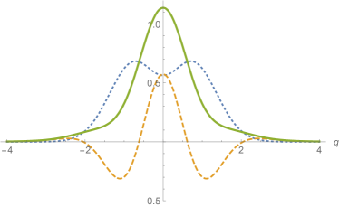
Figure 1: Plot of $n_{B}(p)\hbar/\ell$ as a function of $q=\ell p/\hbar$ (green solid curve) as given by (41). We also display $n_{F}(p)\hbar/\ell$ in (22) (blue dotted curve) and their difference $n_{D}(p)\hbar/\ell$ (40) (orange dashed curve).

IV Tests of the momentum distribution expression (41)

We consider now three tests on the analytical expression of the momentum distribution $n_{B}(p)$. First, we will verify that the correct value of $n_{B}(p=0)$ is obtained, then we will check the normalization condition, and finally we will make sure that we recover the correct high-$p$ asymptotic behavior.

IV.1 Test of $n_{B}(p)$ at zero momentum $p=0$

We wish to compare the value of momentum density $n_{B}(p)$ at $p=0$ by using its definition in (15) with that obtained through our general expression (41). While the idea of the test is simple, the calculations are not straightforward.

Using the definition (15) together with $\rho_{B}(x_{1},x_{2})$ given by the first eqality in (6), gives for $p=0$

$$n_{B}\left(0\right)=\frac{1}{2\pi\hbar}\int_{-\infty}^{\infty}\int_{-\infty}^{\infty}\rho_{B}\left(x_{1},x_{2}\right)dx_{1}dx_{2}=\frac{\ell}{\pi^{2}\hbar}\int_{-\infty}^{\infty}\int_{-\infty}^{\infty}e^{-\frac{(z_{1}^{2}+z_{2}^{2})}{2}}dz_{1}dz_{2}\int_{-\infty}^{\infty}e^{-\xi^{2}}|z_{1}-\xi||z_{2}-\xi|d\xi.$$ (42)

For any fixed value of $\xi$, we make the change of variables $z_{1}=r+\xi$, $z_{2}=s+\xi$, and get

$$n_{B}\left(0\right)=\frac{\ell}{\pi^{2}\hbar}\int_{-\infty}^{\infty}\int_{-\infty}^{\infty}|r|\,|s|e^{-\frac{(r^{2}+s^{2})}{2}}\,drds\int_{-\infty}^{\infty}e^{-2\xi^{2}}e^{-(r+s)\xi}d\xi.$$ (43)

After the integration on $\xi$ is performed, the above expression reduces to

$$n_{B}\left(0\right)=\frac{\ell}{\pi^{3/2}\sqrt{2}\,\hbar}\int_{-\infty}^{\infty}dr\,|r|e^{-\frac{3}{8}r^{2}}\int_{-\infty}^{\infty}ds\,|s|e^{-\frac{3}{8}s^{2}}e^{\frac{rs}{4}}=\frac{\ell\sqrt{2}}{\pi^{3/2}\hbar}\int_{-\infty}^{\infty}dr\,|r|e^{-\frac{3}{8}r^{2}}\int_{0}^{\infty}se^{-\frac{3}{8}s^{2}}\cosh(\tfrac{rs}{4})\,ds.$$ (44)

Using the identity (see eq. (3.562) number (4) of Gradshteyn–Ryzhik )

$$\int_{0}^{\infty}se^{-\beta s^{2}}\cosh(\gamma s)ds=\frac{1}{2\beta}+\frac{\gamma}{4\beta}\sqrt{\frac{\pi}{\beta}}\,e^{\frac{\gamma^{2}}{4\beta}}\,\text{erf}\left(\frac{\gamma}{2\sqrt{\beta}}\right)$$ (45)

for $\beta=3/8,\gamma=r/4$ in (44), we obtain

$$n_{B}(0)=\frac{\ell\sqrt{2}}{\pi^{3/2}\hbar}\int_{-\infty}^{\infty}|r|e^{-\frac{3}{8}r^{2}}dr\left[\frac{4}{3}+\sqrt{\frac{8\pi}{3}}e^{\frac{r^{2}}{24}}\frac{r}{6}\,\text{erf}\left(\frac{r}{4}\sqrt{\frac{2}{3}}\right)\right]=\frac{\ell\sqrt{2}}{\pi^{3/2}\hbar}\left[\frac{32}{9}+\sqrt{\frac{8\pi}{27}}\int_{0}^{\infty}r^{2}e^{-\frac{r^{2}}{3}}\,\text{erf}\left(\frac{r}{4}\sqrt{\frac{2}{3}}\right)\right].$$

The remaining integral can be found in the literature Ng-Gell1969 , and after simplifications we get

$$n_{B}(0)=\frac{\ell}{\sqrt{\pi}\hbar}\left[\frac{4}{\pi}\arctan(\sqrt{2})+\frac{4\sqrt{2}}{\pi}-1\right].$$ (46)

It is interesting to compare this value of the momentum density at $p=0$ (peak momentum distribution) with its two-fermions system counterpart given by (22)

$$n_{F}(0)=\frac{\ell}{\sqrt{\pi}\hbar}.$$ (47)

We clearly observe a large deviation measured by the ratio $n_{B}\left(0\right)/n_{F}(0)=\left[\frac{4}{\pi}\arctan\left(\sqrt{2}\right)+\frac{4\sqrt{2}}{\pi}-1\right]\allowbreak\approx 2.02$. This ratio is featured in fig. 1.

Let us now check that the result (46) is also obtained by setting $p=0$ into expression (41)

$$n_{B}(0)=\frac{\ell}{\sqrt{\pi}\hbar}+\frac{\ell}{\sqrt{\pi}\hbar}\left(\frac{4\sqrt{2}}{\pi}\right)\left[\frac{2}{3}+\Psi_{1}\left(2,\frac{1}{2},\frac{3}{2},\frac{1}{2};-\frac{1}{2},0\right)-\Psi_{1}\left(1,\frac{1}{2},\frac{3}{2},\frac{1}{2};-\frac{1}{2},0\right)\right].$$ (48)

In order to compute $\Psi_{1}\left(1,\frac{1}{2},\frac{3}{2},\frac{1}{2};-\frac{1}{2},0\right)$ and $\Psi_{1}\left(2,\frac{1}{2},\frac{3}{2},\frac{1}{2};-\frac{1}{2},0\right)$, we return to the third form of the confluent hypergeometric function with two variables in (37) and set $z_{2}=0$:

$$\Psi_{1}\left(1,\frac{1}{2},\frac{3}{2},\frac{1}{2};-\frac{1}{2},0\right)={}_{2}F_{1}\left(1,\frac{1}{2},\frac{3}{2};-\frac{1}{2}\right),\qquad\Psi_{1}\left(2,\frac{1}{2},\frac{3}{2},\frac{1}{2};-\frac{1}{2},0\right)={}_{2}F_{1}\left(2,\frac{1}{2},\frac{3}{2};-\frac{1}{2}\right).$$ (49)

To compute ${}_{2}F_{1}\left(1,\frac{1}{2},\frac{3}{2};-\frac{1}{2}\right)$ we use the relation ${}_{2}F_{1}\left(1,\frac{1}{2},\frac{3}{2};-z^{2}\right)=(\arctan z)/z$ (see (9.121) number (27) of ref. Gradshteyn–Ryzhik ), with $z^{2}=1/\sqrt{2}$. Making use of the well known relation $\arctan(z)+\arctan(1/z)=\pi/2$, we find

$${}_{2}F_{1}\left(1,\frac{1}{2},\frac{3}{2};-\frac{1}{2}\right)=\sqrt{2}\arctan(1/\sqrt{2})=\sqrt{2}\left[\frac{\pi}{2}-\arctan(\sqrt{2})\right].$$ (50)

The other quantity ${}_{2}F_{1}\left(2,\frac{1}{2},\frac{3}{2};-\frac{1}{2}\right)$ can be easily obtained by applying the recursion relation (15.2.14) of Abramowitz-Stegun1972 with $a=1$, $b=1/2$ and $c=3/2$:

$$\text{ }_{2}F_{1}\left(2,\frac{1}{2},\frac{3}{2};-\frac{1}{2}\right) = \frac{1}{2}\,_{2}F_{1}\left(1,\frac{1}{2},\frac{3}{2};-\frac{1}{2}\right)+\frac{1}{2}\,_{2}F_{1}\left(1,\frac{3}{2},\frac{3}{2};-\frac{1}{2}\right)$$ (51)

$$= \frac{1}{2}\,_{2}F_{1}\left(1,\frac{1}{2},\frac{3}{2};-\frac{1}{2}\right)+\frac{1}{3}$$

where the second equality is obtained by noting that $\,{}_{2}F_{1}\left(1,b,b;z\right)=1/(1-z)$, here with $z=-1/2$. Substituting (49), together with (50) and (51), into (48), we recover the peak momentum distribution value (46), thus ending the proof.

IV.2 Normalization condition of momentum distribution n${}_{B}(p)$

Next, we want to show that momentum density obeys the normalization condition $\int n_{B}\left(p\right)dp=2$. It is more convenient not to use the form of $n_{B}\left(p\right)$ in (41), but an expression obtained a few steps before. That is, we use the momentum density as given in (17), $n_{B}\left(p\right)=n_{F}(p)+n_{D}(p)$, with the expressions for $n_{F}(p)$ and $n_{D}(p)$ given by (20) and (27), to write

$$n_{B}(p)=\frac{2\ell}{\hbar\pi}\left[\int_{-\infty}^{\infty}e^{-v^{2}}\cos(2qv)dv-\int_{-\infty}^{\infty}v^{2}e^{-v^{2}}\cos(2qv)dv\right]+\frac{4\ell}{\pi^{3/2}\hbar}\left[\sqrt{2}\int_{-\infty}^{\infty}e^{-\frac{3v^{2}}{2}}|v|\cos(2qv)dv\right.\qquad\qquad$$

$$\left.-\sqrt{\pi}\int_{-\infty}^{\infty}e^{-v^{2}}\cos(2qv)\,\text{erf}\left(\frac{|v|}{\sqrt{2}}\right)dv+\sqrt{\pi}\int_{-\infty}^{\infty}e^{-v^{2}}v^{2}\cos(2qv)\,\text{erf}\left(\frac{|v|}{\sqrt{2}}\right)dv\right].$$ (52)

Taking into account the following representation of the Dirac delta distribution

$$\int_{-\infty}^{\infty}\cos(2qv)\,dq=\pi\delta(v),$$ (53)

the integral over the momentum $p$ (or equivalently over $q=\ell p/\hbar$) is quite straightforward

$$\int n_{B}(p)\,dp=2\int_{-\infty}^{\infty}\left[e^{-v^{2}}-v^{2}e^{-v^{2}}+\frac{2\sqrt{2}}{\sqrt{\pi}}e^{-\frac{3v^{2}}{2}}\left|v\right|-2e^{-v^{2}}\,\text{erf}\left(\frac{\left|v\right|}{\sqrt{2}}\right)+2e^{-v^{2}}v^{2}\,\text{erf}\left(\frac{\left|v\right|}{\sqrt{2}}\right)\right]\delta(v)\,dv=2,$$ (54)

where the final result is obtained using $\text{erf}(0)=0$. We have thus checked that, for the two-particle system considered in this work, we have the correct normalization condition for $n_{B}(p)$.

IV.3 High-$p$ behavior of the momentum distribution and Tan’s coefficient

Here, we will examine the asymptotic behavior of the momentum density $n_{B}(p)$ obtained in (41) as $p\rightarrow\infty$ and we will prove that

$$n_{B}(p)\approx\frac{C_{2}}{{}p^{4}},\quad p\rightarrow\infty,\qquad C_{2}=(2m\hbar\omega/\pi)^{3/2}=(2/\pi)^{3/2}\,(\hbar/\ell)^{3},$$ (55)

where $C_{2}$ is the exact Tan’s contact coefficient for the two-atom system under study Tan , recovering the $1/p^{4}$ dependence originated from the short-range character of the interaction.

To derive this result we search the asymptotic behavior up to $1/p^{4}$. For this purpose we need the asymptotic behavior ($x\rightarrow+\infty$) Olver2010

$$M(a,b;-x)\approx\frac{\Gamma(b)}{\Gamma(b-a)}x^{-a}\sum\limits_{k=0}^{\infty}\frac{(1+a-b)_{k}(a)_{k}}{k!}x^{-k},$$ (56)

$a\neq 0,-1,-2,...$

Taking $a=1,b=\frac{3}{2}$ and $x=2\ell^{2}p^{2}/(3\hbar^{2})$, we have from (56) that

$$\frac{4}{3}\left(\frac{\ell p}{\hbar}\right)^{2}M\left(1,\frac{3}{2};-\frac{2}{3}\frac{\ell^{2}p^{2}}{\hbar^{2}}\right)\approx\sum\limits_{k=0}^{\infty}\frac{(\frac{1}{2})_{k}(1)_{k}}{k!}\left(\frac{3\hbar^{2}}{2\ell^{2}p^{2}}\right)^{k}=1+\frac{3}{4}\frac{\hbar^{2}}{\ell^{2}p^{2}}+\frac{27}{16}\frac{\hbar^{4}}{\ell^{4}p^{4}}+O\left(\frac{1}{p^{6}}\right).$$ (57)

To determine the asymptotic behavior of $\Psi_{1}\left(1+j,1/2,3/2,1/2;-1/2,-\ell^{2}p^{2}/\hbar^{2}\right)$ as $p\rightarrow\infty$, with either $j=0$ or $j=1$, we use the second expression in (36) to write

$$\Psi_{1}\left(1+j,\frac{1}{2},\frac{3}{2},\frac{1}{2};-\frac{1}{2},-\frac{\ \ell^{2}p^{2}}{\hbar^{2}}\right)=\sum\limits_{m=0}^{\infty}\frac{(1+j)_{m}(\frac{1}{2})_{m}}{(\frac{3}{2})_{m}}\frac{\left(-\frac{1}{2}\right)^{m}}{m!}M\left(1+j+m,\frac{1}{2};-\frac{\ \ell^{2}p^{2}}{\hbar^{2}}\right)\text{ }$$ (58)

and then the asymptotic expansion (56) to get

$$\Psi_{1}\left(1+j,\frac{1}{2},\frac{3}{2},\frac{1}{2};-\frac{1}{2},-\frac{\ell^{2}p^{2}}{\hbar^{2}}\right)\approx\sum\limits_{m=0}^{\infty} \frac{(1+j)_{m}(\frac{1}{2})_{m}}{(\frac{3}{2})_{m}}\frac{\left(-\frac{1}{2}\right)^{m}}{m!}\frac{\Gamma(\frac{1}{2})}{\Gamma(-m-j-\frac{1}{2})}\ \left(\frac{\ell^{2}p^{2}}{\hbar^{2}}\right)^{-m-j-1}$$ (59)

$$\times\sum\limits_{k=0}^{\infty}\frac{(m+j+\frac{3}{2})_{k}(m+j+1)_{k}}{k!}\left(\frac{\ell^{2}p^{2}}{\hbar^{2}}\right)^{-k}.$$

To retain only terms up to $1/p^{4}$, we have to consider the summation indexes up to $m+k\leq 1-j$. It is easy to show that

$$\Psi_{1}\left(1,\frac{1}{2},\frac{3}{2},\frac{1}{2};-\frac{1}{2},-\frac{\ell^{2}p^{2}}{\hbar^{2}}\right) \approx -\frac{\hbar^{2}}{2\ell^{2}p^{2}}-\frac{7}{8}\frac{\hbar^{4}}{\ell^{4}p^{4}}+O\left(\frac{1}{p^{6}}\right).$$ (60)

$$\Psi_{1}\left(2,\frac{1}{2},\frac{3}{2},\frac{1}{2};-\frac{1}{2},-\frac{\ell^{2}p^{2}}{\hbar^{2}}\right) \approx \frac{3}{4}\frac{\hbar^{4}}{\ell^{4}p^{4}}+O\left(\frac{1}{p^{6}}\right).$$ (61)

Collecting expressions (57), (60) and (61) into (41), after the cancellation of the terms of order $1/p^{2}$, one finds

$$n_{B}\left(p\right)\approx\left(\frac{2\hbar^{3}\sqrt{2}}{\ell^{3}\pi^{\frac{3}{2}}}\right)\frac{1}{p^{4}}=\left(\frac{2m\hbar\omega}{\pi}\right)^{\frac{3}{2}}\frac{1}{p^{4}},$$ (62)

which is the result announced in (55): we have recovered the well known $1/p^{4}$ asymptotic decay of $n_{B}(p)$ for high momentum values. The coefficient in front of the high-$p$ tail of the momentum distribution, called Tan’s coefficient Tan , is given by $(2/\pi)^{3/2}(m\omega\hbar)^{3/2}$ for the system of two particles under study. Note, finally, that from a basic dimensional analysis, expressions in (62) or (55) have correct units of momentum density.

The high-$p$ tail behavior can be observed in fig. 2 where we show $n_{B}(p),n_{F}(p)$ and $n_{D}(p)$ multiplied by $p^{4}/C_{2}$. One can appreciate how $n_{B}(p)$ tends to 1 for large $q$, and that the asymptotic limit is dominated by the deviation term $n_{D}$, since the $n_{F}$ is already negligible for $q>4$.

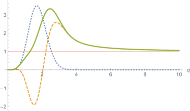
Figure 2: Plot of $n_{B}(p)p^{4}/C_{2}$ (green solid curve), $n_{F}(p)p^{4}/C_{2}$ (blue dotted curve) and $n_{D}(p)p^{4}/C_{2}$ (yellow dashed curve) as a function of $q=\ell p/\hbar$, with $C_{2}=(2/\pi)^{3/2}\,(\hbar/\ell)^{3}$.

V Conclusion

In this paper we have studied a one-dimensional quantum system consisting of two bosons harmonically trapped and with an infinite contact repulsion. This system has been the subject of numerous studies, in particular with respect to its asymptotic momentum distribution. In the present work we have been able to provide an exact expression of the momentum distribution valid for arbitrary value of the momentum, and thus we have extended the list of exactly solvable models of two interacting particles. Starting from the wave function of the two particles, we have derived an exact expression of the one-body density matrix expressed in terms of centre of mass and relative coordinates. From this result we have calculated the corresponding momentum distribution. To clearly identify the deviation of this system from the two noninteracting fermions, we wrote this momentum density as the sum of two terms: a first one corresponding to the two noninteracting fermions, and a second one related to the short range character of the interaction.

In order to validate our analytic expression of the momentum density, three robust tests have been performed satisfactorily. In particular, the third test concerns the asymptotic decay for high momentum values; we have been able to derive the exact expression of the Tan contact coefficient, which we recall is the coefficient in front of the high-$p$ tail of the momentum distribution, for the case of two particles Tan .

Appendix A

In this Appendix we will calculate the two functions $\mathcal{B}(u,v)$ and $\mathcal{C}(u,v)$ given by (10), and thereafter $\mathcal{A}(u,v)$ defined in (9). Making the change of variable $t=w+u$ in $\mathcal{B}(u,v)$, we get

$$\mathcal{B}(u,v)=\int_{-\infty}^{u-\left|v\right|}t^{2}e^{-t^{2}}\,dt-2u\int_{-\infty}^{u-\left|v\right|}\,te^{-t^{2}}\,dt+\left(u^{2}-v^{2}\right)\int_{-\infty}^{u-\left|v\right|}e^{-t^{2}}\,dt.$$ (63)

If we perform an integration by parts in the first integral, we then get after rearrangements

$$\mathcal{B}(u,v)=\frac{1}{2}\left(u+|v|\right)e^{-(u-|v|)^{2}}+\left(\tfrac{1}{2}+u^{2}-v^{2}\right)\int_{-\infty}^{u-|v|}\,e^{-t^{2}}\,dt.$$ (64)

Proceeding similarly for $\mathcal{C}(u,v)$, we write

$$\mathcal{C}(u,v)=\int_{u-\left|v\right|}^{u+\left|v\right|}\,t^{2}e^{-t^{2}}\,dt-2u\int_{u-\left|v\right|}^{u+\left|v\right|}\,te^{-t^{2}}\,dt+\left(u^{2}-v^{2}\right)\int_{u-\left|v\right|}^{u+\left|v\right|}\,e^{-t^{2}}\,dt.$$ (65)

Carrying out an integration by parts of the first integral, transforms (65) as

$$\mathcal{C}(u,v) = \frac{1}{2}\left(u-\left|v\right|\right)e^{-(u+\left|v\right|)^{2}}-\frac{1}{2}\left(u+{\left|v\right|}\right)e^{-(u-{\left|v\right|})^{2}}+\left(\frac{1}{2}+u^{2}-v^{2}\right)\int_{u-\left|v\right|}^{u+\left|v\right|}e^{-t^{2}}\,dt.$$ (66)

Collecting the two results (64) and (66), the expression of $\mathcal{A}(u,v)$ in (9) becomes

$$\mathcal{A}(u,v)=(u+{|v|})e^{-(u-{|v|})^{2}}-(u-{|v|})e^{-(u+{|v|})^{2}}+(\tfrac{1}{2}+u^{2}-v^{2})\left[\int_{-\infty}^{u-\left|v\right|}e^{-t^{2}}dt+\int_{-\infty}^{-u-\left|v\right|}e^{-t^{2}}dt-\int_{u-\left|v\right|}^{u+\left|v\right|}e^{-t^{2}}dt\right].$$

To further simplify, let us observe that

$$\int_{-\infty}^{u-\left|v\right|}e^{-t^{2}}dt+\int_{-\infty}^{-u-\left|v\right|}e^{-t^{2}}dt=\int_{-\infty}^{\infty}e^{-t^{2}}dt-\int_{u-\left|v\right|}^{u+\left|v\right|}e^{-t^{2}}dt=\sqrt{\pi}-\int_{u-\left|v\right|}^{u+\left|v\right|}e^{-t^{2}}\,dt.$$ (67)

Using the definition of the erf function $\int\nolimits_{0}^{a}e^{-t^{2}}dt=\frac{1}{2}\sqrt{\pi}\,\text{erf}(a)$, we further have

$$\int_{u-\left|v\right|}^{u+\left|v\right|}e^{-t^{2}}dt=\frac{\sqrt{\pi}}{2}\bigl{(}\text{erf}\left(u+\left|v\right|\right)-\text{erf}\left(u-\left|v\right|\right)\bigr{)}.$$ (68)

Combining the above two results, the expression of $\mathcal{A}(u,v)$ becomes

$$\mathcal{A}(u,v)=(u+{|v|})e^{-(u-{|v|})^{2}}-(u-{|v|})e^{-(u+{|v|})^{2}}+\sqrt{\pi}(\tfrac{1}{2}+u^{2}-v^{2})\bigl{(}1+\text{erf}\left(u-\left|v\right|\right)-\text{erf}\left(u+\left|v\right|\right)\bigr{)}.$$ (69)

Appendix B

In this Appendix we consider the double integral $I_{2}$ in (25)

$$I_{2}=\frac{4\ell}{\pi^{3/2}\hbar}\int_{-\infty}^{\infty}e^{-v^{2}}\cos(2qv)\,dv\int_{-\infty}^{\infty}\left(\tfrac{1}{2}-v^{2}+u^{2}\right)\,\text{erf}\left(u-|v|\right)\,e^{-u^{2}}du=\frac{4\ell}{\pi^{3/2}\hbar}\,(K_{1}+K_{2}+K_{3}),$$ (70)

which, for convenience, we have split into three double integrals defined through

$$K_{1} = \frac{1}{2}\int_{-\infty}^{\infty}e^{-{v^{2}}}\cos(2qv)dv\int_{-\infty}^{\infty}e^{-u^{2}}\text{erf}\left(u-{|v|}\right)du,$$ (71)

$$K_{2} = -\int_{-\infty}^{\infty}v^{2}e^{-{v^{2}}}\cos(2qv)dv\int_{-\infty}^{\infty}e^{-u^{2}}\text{erf}\left(u-{|v|}\right)du,$$ (72)

$$K_{3} = \int_{-\infty}^{\infty}e^{-{v^{2}}}\cos(2qv)dv\int_{-\infty}^{\infty}u^{2}e^{-u^{2}}\text{erf}\left(u-{|v|}\right)du.$$ (73)

In order to compute the $u$ integral in (73), we first perform an integration by parts to get

$$G=\int_{-\infty}^{\infty}u^{2}e^{-u^{2}}\text{erf}\left(u-|v|\right)du=\frac{1}{2}\int_{-\infty}^{\infty}e^{-u^{2}}\text{erf}\left(u-|v|\right)du+\frac{1}{\sqrt{\pi}}\int_{-\infty}^{\infty}e^{-u^{2}}ue^{-\left(u-|v|\right)^{2}}du.$$ (74)

The second integral on the right-hand side of (74) can be carried out, giving

$$G=\frac{1}{2}\int_{-\infty}^{\infty}e^{-u^{2}}\text{erf}\left(u-|v|\right)du+\frac{|v|}{2\sqrt{2}}e^{-|v|^{2}/2}.$$ (75)

Hence, substituting (75) into (73), one finds out that $K_{3}$ is related to $K_{1}$ through

$$K_{3}=K_{1}+\frac{1}{\sqrt{2}}\int_{0}^{\infty}e^{-3v^{2}/2}\,v\,\cos(2qv)\,dv.$$ (76)

To carry out the $u$ integrals in (71)–(72), we start from the identity

$$\int_{-\infty}^{\infty}e^{-(x+a)^{2}}\text{erf}\left(x\right)dx=-\sqrt{\pi}\,\text{erf}\left(\frac{a}{\sqrt{2}}\right)=\int_{-\infty}^{\infty}e^{-t^{2}}\text{erf}\left(t-a\right)dt.$$ (77)

Using the above relation for $a=|v|$ allows us to write the expressions of (71) and (72) as single integrals, so that

$$K_{1}=-\sqrt{\pi}\int_{0}^{\infty}e^{-{v^{2}}}\cos(2qv)\,\text{erf}\left(\frac{v}{\sqrt{2}}\right)dv,\qquad K_{2}=2\sqrt{\pi}\int_{0}^{\infty}v^{2}e^{-v^{2}}\cos(2qv)\,\text{erf}\left(\frac{v}{\sqrt{2}}\right)dv.$$ (78)

Finally adding the three results (78) and (76), we can write (70) as

$$I_{2} = \frac{4\ell}{\pi^{3/2}\hbar}\left\{-2\sqrt{\pi}\int_{0}^{\infty}e^{-v^{2}}\cos(2qv)\,\text{erf}\left(\frac{v}{\sqrt{2}}\right)dv\right.$$

$$\qquad\qquad\left.+2\sqrt{\pi}\int_{0}^{\infty}v^{2}e^{-v^{2}}\cos(2qv)\,\text{erf}\left(\frac{v}{\sqrt{2}}\right)dv+\frac{\sqrt{2}}{2}\int_{0}^{\infty}e^{-3v^{2}/2}\,v\,\cos(2qv)\,dv\right\}.$$

References

• (1) T. Kinoshita, T. Wenger, D.S. Weiss, Science 305, 1125 (2004)
• (2) M.D. Girardeau, J. Math. Phys. 1, 516 (1960)
• (3) M.D. Girardeau, E.M. Wright, Phys. Rev. Lett. 84, 5691 (2000)
• (4) M.D. Girardeau, E.M. Wright, J.M. Triscari, Phys. Rev. A 63, 033601 (2001); G.J. Lapeyre, M.D. Girardeau, E.M. Wright, Phys. Rev. A 66, 023606 (2002)
• (5) F. Deuretzbacher, D. Becker, J. Bjerlin, S.M. Reimann, L. Santos, Phys. Rev. A 90, 013611 (2014)
• (6) A.G. Volosniev, D.V. Fedorov, A.S. Jensen, M. Valiente, N.T. Zinner, Nature Communications 5, 5300 (2014)
• (7) A.G. Volosniev, D. Petrosyan, M. Valiente, D.V. Fedorov, A.S. Jensen, N.T. Zinner, Phys. Rev. A 91, 023620 (2015)
• (8) S.S. Alam, T. Skaras, Li. Yang, H. Pu, Dynamical Fermionization in One Dimensional Spinor Gases (2020). arXiv:2008.08383v1 [cond-mat.quant-gas]
• (9) M. Olshanii, V. Dunjko, Phys. Rev. Lett. 91, 090401 (2003)
• (10) S. Tan, Ann. Phys. 323, 2952 (2008); 323, 2971 (2008); 323, 2987 (2008).
• (11) R.M. Dreizler, E.K.U. Gross, Density Functional Theory: An Approach to the Quantum Many-Body Problem (Springer-Verlag, Berlin, 1990)
• (12) R. Pezer, H. Buljan, Phys. Rev. Lett. 98, 240403 (2007)
• (13) R. Boumaza, Dynamical properties of quantum gases following a sudden change of confining potential, Doctoral Thesis (UFA, Sétif, 2019)
• (14) P. Vignolo and A. Minguzzi, Phys. Rev. Lett. 110, 020403 (2013)
• (15) I.S. Gradshteyn, I.M. Ryzhik, Table of Integrals, Series and Products (Academic Press, New York, 1994)
• (16) C. Cohen-Tannoudji, B. Diu, F. Laloë, Quantum Mechanics, Volume 1: Basic Concepts, Tools, and Applications (Wiley-VCH, Weinheim, 2019)
• (17) A.P. Prudnikov, U.I.A. Brychkov, O.I. Marichev, Integrals and series. Vol 2, Special functions (Gordon and Breach Science Publishers, New York (NY), 1986)
• (18) H.M. Srivastava, P.W. Karlsson, Multiple Gaussian Hypergeometric Series (Ellis Horwood, Chichester, 1985)
• (19) L.U. Ancarani, J.A. Del Punta, G. Gasaneo, J. Math. Phys. 58, 073504 (2017)
• (20) E. W. Ng and M. Gell, A table of integrals of error functions, Journal of research of the National Bureau of Standards - B. Mathematical Sciences Vol. 73B, 1 (1969)
• (21) M. Abramowitz, I. A. Stegun, Handbook of Mathematical Functions (Dover, New York, 1972)
• (22) F.W.J. Olver, D.W. Lozier, R.F. Boisvert, C.W. Clark (eds.), NIST Handbook of Mathematical Functions (Cambridge University Press, Cambridge, 2010)