FDG: A Precise Measurement of Fault Diagnosability Gain of Test Cases

Abstract.

The performance of many Fault Localisation (FL) techniques directly depends on the quality of the used test suites. Consequently, it is extremely useful to be able to precisely measure how much diagnostic power each test case can introduce when added to a test suite used for FL. Such a measure can help us not only to prioritise and select test cases to be used for FL, but also to effectively augment test suites that are too weak to be used with FL techniques. We propose FDG, a new measure of Fault Diagnosability Gain for individual test cases. The design of FDG is based on our analysis of existing metrics that are designed to prioritise test cases for better FL. Unlike other metrics, FDG exploits the ongoing FL results to emphasise the parts of the program for which more information is needed. Our evaluation of FDG with Defects4J shows that it can successfully help the augmentation of test suites for better FL. When given only a few failing test cases (2.3 test cases on average), FDG can effectively augment the given test suite by prioritising the test cases generated automatically by EvoSuite: the augmentation can improve the acc@1 and acc@10 of the FL results by 11.6x and 2.2x on average, after requiring only ten human judgements on the correctness of the assertions EvoSuite generates.

1. Introduction

Fault Localisation (FL) techniques aim to reduce the cost of software debugging by automatically identifying the root cause of the observed test failures (Wong et al., 2016). While some FL techniques use only static data such as lexical proximity between bug reports and source code (Saha et al., 2013), the majority of FL techniques are based on dynamic analysis: Spectrum Based Fault Localisation (SBFL) relies on both the test coverage and the test results (Jones and Harrold, 2005; Naish et al., 2011; Wong et al., 2014), whereas Mutation Based Fault Localisation exploits the relationship between mutants and test cases (Moon et al., 2014; Hong et al., 2017; Papadakis and Traon, 2015; Papadakis and Le-Traon, 2012). In both cases, the quality of the test suite used with an FL technique can significantly affect its performance. It is widely known that FL techniques thrive only when accompanied by a rich and diverse test suite (Perez et al., 2017).

In reality, however, it is not always the case that the given test suite is sufficiently diverse to ensure successful fault localisation. In fact, it is not unusual to start the debugging process only with a single failing test input, calling for the need of test augmentation. Many techniques have been developed to guide the test augmentation, i.e., to add the test case that can maximise the diagnosability of the augmented test suite (Campos et al., 2013; Artzi et al., 2010). Equally relevant are the techniques that prioritise the given test cases for better and earlier fault localisation (Yoo et al., 2013; Gonzalez-Sanchez et al., 2010), as well as techniques that aim to measure the diagnostic capability of the given test suite. Most of these techniques are built around a metric that measures the diagnosability of either a single test, or a set of tests. However, our analysis of existing test diagnosability metrics reveals room for improvement. Specifically, while some of the techniques are result-aware, i.e., incorporate the result of test executions (pass/fail) into the diagnosability computation, none of them directly uses the suspiciousness scores of individual program elements during localisation, even though they can provide critical information by pinpointing where the prioritisation should focus on next.

Based on our analysis of existing techniques, we propose FDG, a metric that can precisely measure the Fault Diagnosability Gain that a test case can bring to a test suite. FDG is designed to be used during fault localisation, and uses the current suspiciousness scores to precisely capture which part of the target program requires additional diagnostic information from the test case under consideration. We first evaluate FDG with developer-written test cases in Defects4J, i.e., under existing and reliable test oracles and with all test coverage available, to study its performance under an ideal setting. We construct fixed-sized test suites by adding test cases in the descending order of their diagnosability measured by FDG and other existing metrics. Test suites constructed based on FDG produce much more accurate fault localisation, achieving acc@10 values that are 23% and 14% higher than those produced by the state-of-the-art metrics.

In a more realistic setting, we also evaluate FDG using automatically generated test cases to augment the initial set of failing test inputs. We posit that the true cost of test suite augmentation is not the cost of test data generation, as it can be automated. Rather, the major cost of test augmentation is the human effort required to produce the test oracles for the generated test data. Our evaluation of FDG assumes an iterative FL scenario, in which an insufficient test suite is augmented, on the fly, with test data automatically generated by EvoSuite. Here, FDG is used to choose the next test case to be presented to the human engineer for the oracle labelling. We show that after only ten interactions with the human engineer, FDG can boost acc@1 and acc@10 by 11.6 (from 5 to 58) and 2.2 (from 63 to 147) times, respectively, compared to the initial test suites that contain only a few failing test cases. In addition, we also show that FDG is fairly resilient to labelling errors with an error rate of up to 30%.

The main contributions of this paper are as follows:

• We analyse, and empirically compare, existing metrics that measure the diagnosability of test cases for fault localisation. Our evaluation compares how quickly existing metrics can improve the accuracy of SBFL techniques by prioritising the human-written test cases in Defects4J.

• We propose a novel diagnosability metric for fault localisation, FDG, based on the analysis of existing metrics. FDG distinguishes itself from existing metrics in that it actively uses the available suspiciousness scores to capture which part of the target program needs additional diagnostic information while localisation is ongoing.

• We first evaluate FDG with human-written tests, to investigate its performance under perfect test oracles. When forced to use a limited number of test cases, using those chosen by FDG can achieve up to 23% higher acc@10 when compared to the localisation driven by state-of-the-art metrics.

• We also report findings from a more realistic scenario, where the developer labels oracles that are generated by EvoSuite to augment an initial set of failing inputs for fault localisation: we use FDG to choose which test data to present to the human engineer for test oracle labelling. FDG can boost acc@1 by 11.6 times after only ten human labels.

• We make our replication package publicly available at: https://github.com/agb94/FDG-artifact (An, 2022)

The remainder of the paper is organised as follows. Section 2 presents the basic notations that will be used throughout the paper, as well as the fundamental concepts in SBFL. Section 3 analyses existing diagnosability metrics and presents a comparison of their performance using human-written tests in Defects4J. Section 4 proposes our novel metric, FDG, based on our analysis. Section 5 describes the experimental setup for our empirical evaluation, the results of which are presented in Section 6. Section 7 discusses implications of this work, while Section 8 presents the related work, and Section 9 considers threats to validity. Finally, Section 10 concludes.

2. Preliminaries

This section introduces the basic notations, the background of SBFL techniques, and the definition of ambiguity groups.

2.1. Basic Notation

Given a program $P$, let us define the following:

• Let $E=\{e_{1},\ldots,e_{n}\}$ be the set of program elements that consist $P$, such as statements or methods, and $T=\{t_{1},\ldots,t_{m}\}$ be the test suite for $P$.

• Let $C_{T}$ be the $m\times n$ coverage matrix of $T$:

  $$C_{T}=\left[\begin{array}[]{cccc}a_{11}&\cdots&a_{1n}\\ \vdots&\ddots&\vdots\\ a_{m1}&\cdots&a_{mn}\end{array}\right]\in\mathbb{B}^{m\times n}$$

  where $C_{T}[i,j]=a_{ij}=1$ if $t_{i}$ covers $e_{j}$ and 0 otherwise.

• Given an arbitrary test case $t$, let $c_{t}\in\mathbb{B}^{1\times n}$ be the coverage vector of $t$, where $c_{t}[j]=1$ if $t$ executes $e_{j}$, and 0 otherwise.

• Let $R:T\rightarrow\mathbb{B}$ be the function that maps a test in $T$ to its result: $R(t)=0$ if $t$ reveals a fault in $P$, and 1 otherwise. Subsequently, the set of failing tests, $T_{f}$, can be defined as $\left\{t\in T|R(t)=0\right\}$. $P$ is faulty when $T_{f}$ is not empty.

2.2. Spectrum-based Fault Localisation (SBFL)

SBFL is a statistical approach for the automated localisation of software faults (Wong et al., 2016). It utilises program spectrum, a summary of the runtime information collected from the program executions, to find the faulty program elements. A representative program spectrum of a program element $e_{j}\in E$ consists of four values: $(e_{p},n_{p},e_{f},n_{f})=(N_{11},N_{01},N_{10},N_{00})$ where

$$N_{ab}=|\left\{t_{i}\in T|C_{T}[i,j]=a\land R(t_{i})=b\right\}|$$

SBFL statistically estimates the suspiciousness of each program element based on the following rationale: “The more the execution of an element is correlated with failing tests (high $e_{f}$, low $n_{f}$) and less with passing ones (high $n_{p}$, low $e_{p}$), the more suspicious the program element is, and vice versa”. A risk evaluation formula $S:\mathbb{I}^{4}\rightarrow\mathbb{R}$ is a formula that converts the four program spectrum values to a suspiciousness score. Many risk evaluation formulas (Abreu et al., 2006; Jones and Harrold, 2005; Naish et al., 2011; Wong et al., 2014) have been designed to implement this core idea. For example, Ochiai (Abreu et al., 2006), one of the most widely studied risk evaluation formulas, computes the suspiciousness as follows:

(1) $$Ochiai(e_{p},n_{p},e_{f},n_{f})=e_{f}/\sqrt{(e_{f}+n_{f})\times(e_{f}+e_{p})}$$

Fig. 1 illustrates a concrete example of calculating Ochiai scores from the coverage matrix and test results.

SBFL is one of the most widely studied FL techniques (Wong et al., 2016) as it is applicable as long as test coverage is available. Due to the applicability, SBFL scores are often used as features for more complicated learn-to-rank FL techniques (Sohn and Yoo, 2017; Li et al., 2019; B. Le et al., 2016), motivating us to improve its effectiveness.

2.3. Ambiguity Groups

An ambiguity group (Stenbakken et al., 1989; Gonzalez-Sanchez et al., 2011a) is a set of program elements that are only executed by the same set of test cases. Given a program $P$ and its elements $E$, we define $AG(T)$ as a set of such ambiguity groups under the test suite $T$. The size of $AG(T)$ is equal to the number of unique columns in $C_{T}$. More formally, $AG(T)$ is a partition (Halmos, 2017) of the set $E$ that satisfies the following properties:

1. $\forall e\in E\ldotp\exists g\in AG(T)\ldotp e\in g$

2. $\forall g\in AG(T)\ldotp\forall e_{i},e_{j}\in g\ldotp C_{T}[:,i]=C_{T}[:,j]$

3. $\forall g_{1},g_{2}\in AG(T)\ldotp g_{1}\neq g_{2}\land e_{i}\in g_{1}\land e_{j}\in g_{2}\\ \implies C_{T}[:,i]\neq C_{T}[:,j]$

Elements in the same ambiguity groups are assigned the same suspiciousness score, since their program spectra are identical. For example, in Fig. 1, $AG(\{t_{1},t_{2},t_{3}\})$ is $\left\{\left\{e_{1},e_{2}\right\},\left\{e_{3},e_{4}\right\},\left\{e_{5}\right\}\right\}$, and all the elements in an ambiguity group are tied in the final ranking and hence cannot be uniquely diagnosed as faulty. Therefore, the performance of an SBFL technique increases when there are more ambiguity groups, and their size is smaller.

Program Elements		$e_{1}$	$e_{2}$	$e_{3}$	$e_{4}$	$e_{5}$
Tests	$t_{1}$					$\bullet$	PASS
	$t_{2}$	$\bullet$	$\bullet$	$\bullet$	$\bullet$		FAIL
	$t_{3}$			$\bullet$	$\bullet$		FAIL
Spectrum	$e_{p}$	0	0	0	0	1
	$n_{p}$	1	1	1	1	0
	$e_{f}$	1	1	2	2	0
	$n_{f}$	1	1	0	0	2
Ochiai		0.71	0.71	1.00	1.00	0.00
Rank		4	4	2	2	5
Additional Tests	$t_{1}^{\prime}$					$\bullet$	PASS
	$t_{2}^{\prime}$	$\bullet$				$\bullet$	PASS
	$t_{3}^{\prime}$	$\bullet$	$\bullet$	$\bullet$	$\bullet$		FAIL
	$t_{4}^{\prime}$			$\bullet$			FAIL
Ochiai	w/ $t_{1}^{\prime}$	0.71	0.71	1.00	1.00	0.00
	w/ $t_{2}^{\prime}$	0.50	0.71	1.00	1.00	0.00
	w/ $t_{3}^{\prime}$	0.82	0.82	1.00	1.00	0.00
	w/ $t_{4}^{\prime}$	0.71	0.71	1.00	0.82	0.00

Figure 1. A simple motivating example with one faulty element $e_{3}$. The dots ($\bullet$) show the coverage relation, and the ranks are computed using the max tie-breaker.

A simple motivating example (The dots ($\bullet$) show the coverage relation, and the ranks are computed using the max tie-breaker.)

3. Analysis of Existing Diagnosibility Metrics

Fig. 1 contains a motivating example that shows the role of a diagnosability metric in FL. In the existing SBFL results based on original test cases $\{t_{1},t_{2},t_{3}\}$, program elements $e_{3}$ and $e_{4}$ form an ambiguity group. They share the highest suspiciousness score, i.e., 1.0, even though only $e_{3}$ is the actual faulty element. In this case, to further distinguish which one is more suspicious between them, we need an additional test case that can break the ambiguity group, i.e., covering either one of the program elements.

Let us now consider the four additional test cases, $t_{1}^{\prime}$ to $t_{4}^{\prime}$, to augment the existing test suite. Adding $t_{1}^{\prime}$ or $t_{3}^{\prime}$ does not provide additional diagnostic information, as the program elements in the same ambiguity group are either executed or not executed together. In comparison, $t_{2}^{\prime}$ and $t_{4}^{\prime}$ can provide more information because they can break an ambiguity group, $\{e_{1},e_{2}\}$ and $\{e_{3},e_{4}\}$, respectively. Between them, $t_{4}^{\prime}$ should be prioritised over $t_{2}^{\prime}$ since the ambiguity group $\{e_{3},e_{4}\}$ is currently more suspicious than $\{e_{1},e_{2}\}$. Fig. 1 shows how Ochiai scores change as each test case is added to the original test suite. When $t_{4}^{\prime}$ is added, the faulty element $e_{3}$ is finally ranked at top as the suspiciousness score of the non-faulty element $e_{4}$ decreases. Quantifying such diagnostic contribution made by individual test cases can inform our test suite augmentation, or even the order of test execution.

There are many existing diagnosability metrics that are designed to capture the information gain contributed by individual test cases. In many cases, these metrics are used as part of a test prioritisation technique that is designed to achieve more accurate fault localisation earlier, or with fewer test cases (Hao et al., 2010; Gonzalez-Sanchez et al., 2011b; Yoo et al., 2013). We can also derive such metrics from diagnosability measures of the entire test suites (Perez et al., 2017; Baudry et al., 2006) by looking at the difference in diagnosability gain achieved by the addition a single test. To the best of our knowledge, these metrics have never been directly compared to each other using the same benchmark. The remainder of this section describes existing diagnosability metrics, and empirically compares them using Defects4J, a collection of real-world faults in Java programs.

3.1. Analysis of Existing Diagnosability Metrics

We analyse nine diagnosability metrics for SBFL from the relevant literature published after 2010. Two of these are simply coverage based Test Case Prioritisation (Yoo and Harman, 2012) techniques that serve as baselines. Out of the seven remaining metrics, four metrics have been introduced as part of test prioritisation techniques that aim to improve FL performance, while the remaining three are derived from the diagnostic capability metrics for entire test suites. Given a diagnosability metric $f$, we use the notation $f(T,t)$ to denote the estimated diagnosability gain brought by a newly chosen single test case $t$ to the set of already executed test cases $T$.

3.1.1. Test Case Prioritisation Metrics

Since SBFL techniques are based on an aggregation of test coverage, we include two coverage-based test case prioritisation techniques, total and additional (Rothermel et al., 1999; Elbaum et al., 2002), as baselines. Total prioritisation greedily selects the test case with the highest coverage over all program elements, while additional prioritisation favours the test case with the highest coverage over remaining uncovered program elements only:

$$\text{Total}(T,t)=|\left\{e_{j}\in E|c_{t}[j]=1\right\}|$$

$$\text{Add}(T,t)=|\left\{e_{j}\in E|c_{t}[j]=1\land\forall t_{i}\in T\ldotp C_{T}[i,j]=0\right\}|$$

In both cases, our rationale is that increasing coverage as early as possible may lead to an earlier increase in the amount of information provided to SBFL techniques.

Renieris and Reiss proposed Nearest Neighbours fault localisation (Renieres and Reiss, 2003), which selects the passing test cases whose execution trace is the closest to the given failing execution. They use a program-dependency-based metric to measure the proximity. Motivated by this work, Bandyopadhyay et al. put weights to test cases using the average of Jaccard similarity between the coverage of a given test case and the failing ones (Bandyopadhyay and Ghosh, 2011). Although Bandyopadhyay et al. do not use this metric to prioritise test cases, we include the metric since it aims to measure the diagnosability of individual test cases. We call this metric as Prox hereafter:

$$\text{Prox}(T,t)=\frac{\sum_{t_{i}\in T_{f}}Jaccard(C_{T}[i,:],c_{t})}{|T_{f}|}$$

Hao et al. (Hao et al., 2010) select a representative subset of test cases from a given test suite to reduce the oracle cost (i.e., to reduce the number of outputs to inspect). Among the three coverage-based strategies introduced, S1, S2, and S3, the most effective one for fault localisation was S3: it takes into account the relative importance of ambiguity groups, which in turn is defined as the ratio of failing tests that execute each group, $pri(g)=e_{f}/(e_{f}+n_{f})$.

$$\text{S3}(T,t)=\sum_{g\in AG^{\prime}(T)}pri(g)\cdot div(t,g)$$

where $AG^{\prime}$ denotes a variation of ambiguity group, which includes program elements that share the same spectrum values, and $div(t,g)$ denotes the size of the smaller subset when $t$ is used to divide $g$ to two subsets based on coverage, i.e., the minimum between $|\{e_{j}\in g|c_{t}[j]=1\}|$ and $|\{e_{j}\in g|c_{t}[j]=0\}|$. Therefore, S3 assigns higher priority to tests that can more evenly split the more important ambiguity groups.

RAPTER (Gonzalez-Sanchez et al., 2011a) prioritises test cases by the amount of ambiguity group reduction achieved by individual test cases. While the aim of reducing ambiguity group is similar to S3, RAPTER considers only the size of ambiguity groups, and not the test results. Here, $p(g)=|g|/n$ is the probability that $g$ contains a faulty element, which is assigned in proportion to the size of the group, and $\frac{|g|-1}{2}$ refers to the expected wasted effort if a developer considers program elements in $g$ randomly.

$$\text{RAPTER}(T,t)=-\sum_{g\in AG(T\cup\left\{t\right\})}p(g)\cdot\frac{|g|-1}{2}$$

FLINT (Yoo et al., 2013) is an information-theoretic approach that formulates test case prioritisation as an entropy reduction process. In FLINT, a test case is given higher priority when it is expected to reduce more entropy (H) (Shannon, 1948) in the suspiciousness distribution across program elements. The expected entropy reduction of each test case is predicted based on the conditional probability of the test case failing; the probability of a new test case failing is approximated as the failure rate observed among the test cases executed so far.

$$\text{FLINT}(T,t)=-\alpha\cdot H(P_{f})-(1-\alpha)\cdot H(P_{p})$$

Here, $\alpha$ is the observed failure rate, $|T_{f}|/|T|$, and $P_{p}$ and $P_{f}$ are the suspiciousness distributions of $T\cup\left\{t\right\}$, computed under the assumption that $t$ passes and fails, respectively. The suspiciousness distributions are computed by normalising the Tarantula (Jones and Harrold, 2005) scores. Among the studied existing metrics, FLINT is the only one that does use suspiciousness scores to measure the diagnosability of a new test to execute. However, it only considers the overall distribution of suspiciousness via Shannon entropy, and does not use scores of individual program elements to focus the prioritisation. Note that we negate the original RAPTER and FLINT metrics so that a higher score means a higher diagnosability gain.

3.1.2. Test Suite Diagnosability Metrics

This section describes test suite diagnosability metrics that are designed to measure the diagnosability of entire test suites. Despite originally being designed for test suites, a test suite diagnosability metric $F$ can also be used to quantify the diagnosability gain of an individual test, $t$, by computing the difference between the diagnosability of an original test suite, $F(T)$, and that of the enhanced test suite, $F(T\cup\left\{t\right\})$:

$$f(T,t)=F(T\cup\left\{t\right\})-F(T)$$

Baudry et al. (Baudry et al., 2006) analysed the features of a test suite that are related to the fault diagnosis accuracy and introduced the Test-for-Diagnosis (TfD) metric that measures the number of ambiguity groups (referred to as Dynamic Basic Blocks (DBB) in their paper). They proposed composing a test suite that maximises the number of DBBs for high diagnosability.

$$\text{TfD}(T)=|AG(T)|$$

EntBug (Campos et al., 2013) evaluates a test suite based on its coverage matrix density, which is defined as the ratio of ones in the coverage matrix. EntBug augments an existing test suite with additionally generated test cases with the goal of balancing the density of the coverage matrix to 0.5.

$$\text{EntBug}(T)=1-|1-2\cdot\rho\left(T\right)|$$

where $\rho\left(T\right)=\sum C_{T}[i,j]/(|E|\cdot|T|)$. Note that this definition is the normalised version (Perez et al., 2017) of EntBug.

More recently, Perez et al. propose DDU (Perez et al., 2017), a test suite diagnosability metric for SBFL, that combines three key properties, density, diversity, and uniqueness, all being properties that a test suite should exhibit to achieve high localisation accuracy. The density component is identical to EntBug, while the uniqueness component is the ratio of the number of ambiguity groups over the number of all program elements, i.e., $|AG(T)|/|E|$. Lastly, the diversity component is designed to ensure the diversity of test executions, i.e., the contents of the rows in the coverage matrix. Formally, it is defined as the Gini-Simpson index (Jost, 2006) among the rows.

$$\text{DDU}(T)=\text{density}(T)\times\text{diversity}(T)\times\text{uniqueness}(T)$$

3.1.3. Classification of Diagnostic Capability Metrics

Among the aforementioned metrics, some can be calculated with only the test coverage, while others require the test results plus the coverage. Thereby, we broadly classify them into two categories based on the utilised information:

• Result-Agnostic: metrics utilising only coverage information; total coverage, additional coverage, RAPTER, TfD, EntBug, and DDU belong to this category.

• Result-Aware: metrics utilising coverage information and previous test results; Prox, S3, and FLINT belong here.

When we order tests according to diagnosability metrics, the result-agnostic metrics are not affected by the results of previously chosen, whereas the result-aware metrics are.

3.2. Evaluation of Existing Metrics

We empirically compare and analyse the performance of existing metrics by studying how much each metric can accelerate fault localisation of real world bugs. For this, we apply the studied existing metrics to the bugs and human-written test cases in the version 2.0 of Defects4J, a widely studied real world fault benchmark (for details about subject programs and bugs, please refer to Section 5.2). We adopt a ranking-based evaluation protocol stated below: while there are questions about whether the ranking form is the most effective way for humans to consume results of FL techniques (Parnin and Orso, 2011), we posit that test suites capable of producing more accurate rankings are also capable of providing higher diagnosibility due to the diversity in its coverage.

3.2.1. Protocol

For every studied fault, we create a test suite that initially only contains one of the failing test cases provided by Defects4J: therefore, we create multiple such test suites based on a single Defects4J fault, if it has multiple failing test cases. Subsequently, we iteratively add ten test cases from the remaining test cases, in the order given by one of the studied existing metrics: after each iteration, we evaluate the accuracy of fault localisation performed using test cases added up to that point. In total, we study 810 test orderings generated from 351 studied faults.

To evaluate the SBFL accuracy at each iteration, we compute the line level Ochiai (Eq. 1) scores, and aggregate them at the method level (Sohn and Yoo, 2017) by assigning each method the score of its most suspicious line. We use max-tiebreaker to break ties in the ranking. Finally, we use Mean Average Precision (mAP) to compare rankings produced by different metrics. mAP is a widely used metric in Information Retrieval, and is defined as the Average Precision (AP) values across multiple queries (in our case, multiple test orderings). Average Precision, in turn, stands for the average of precision values at each rank of all positive samples (in our case, faulty methods). For example, if a program contains two faulty methods, A and B, placed at the second and the fifth places, the AP is $\frac{1}{2}(\frac{1}{2}+\frac{2}{5})=0.45$: the higher the mAP value is, the better the overall ranking is.

3.2.2. Comparison Results

Figure 2 shows the trends of mAP values produced by different metrics at each iteration. Lines are colour-coded for each metric; metrics in result-agnostic and result-aware categories are shown in solid and dashed lines, respectively. While we only show the results for the first ten iterations, note that the mAP values will eventually converge to the same value per a Defects4J fault, as the Ochiai ranking produced using all test cases should be identical w.r.t. a deterministic tie-breaker. A metric is more effective if the line converges faster.

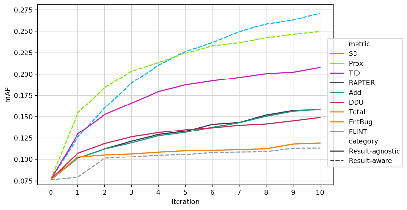
The mAP values for each prioritisation metric during ten iterations

Figure 2. The mAP values for each prioritisation metric during ten iterations

The results show that two result-aware metrics, S3 and Prox, outperform all other result-agnostic metrics. With S3, the initial mAP value, $0.076$, is increased to $0.271$ (an increase of 257%) after the ten test cases are selected, whereas TfD, the best performing result-agnostic metric, only achieves 172% improvement during the same number of iterations. Prox, which sorts test cases by their similarity to failing tests, shows faster initial convergence, while S3 achieves higher localisation performance after the fifth iteration. Both S3 and TfD, metrics that aim to split ambiguity groups, show the best result at the tenth iteration among the result-aware and result-agnostic metrics, respectively. Compared to S3 and Prox, FLINT does not perform as well, despite being a result-aware metric. FLINT is originally designed to initially prioritise for coverage and switch to prioritisation for fault localisation once a test fails, whereas our evaluation scenario starts with a failing test case. Consequently, the observed failure rate starts at 1.0 for FLINT, which significantly skews its following analysis.

Among the result-agnostic metrics, Total and EntBug perform identically on our subjects. Total gives higher priority to tests that cover more program elements. Similarly, EntBug also takes into account the number of covered program elements, while aiming to reach the optimal density of 0.5. However, since the level of coverage achieved by individual human-written test cases in our subject is fairly low, EntBug ends up trying to increase the coverage for all ten iterations, which in turn increases the density. Another interesting observation is that TfD outperforms DDU, even though TfD is conceptually identical to the uniqueness component of DDU. DDU gives high priority to test cases that are either not similar to existing failing test cases or cover more elements, thanks to the diversity and the density metrics. However, the results of Prox show that choosing tests similar to failing tests can be effective, while Total and EntBug show that relying on coverage density alone may not be effective. Based on this, we posit that, when a failing test already exists and is known, it is better to prioritise tests that are similar to the failing test than to focus on test diversity.

In summary, our evaluation using Defects4J shows that two result-aware metrics, S3 and Prox, outperform all result-agnostic metrics. When diagnosing faults that have already been observed by failing executions, result-agnostic metrics cannot efficiently prioritise test cases because they cannot distinguish the more suspicious elements from those that are less so.

4. Fault Diagnosibility Gain

This section proposes a novel diagnosability metric, FDG (Fault Diagnosibility Gain), that better measures the fault diagnosability gain by leveraging the ongoing FL results during the prioritisation.

4.1. Design of FDG (Fault Diagnosability Gain)

Our new diagnosability metric, FDG, consists of two subcomponents, Split and Cover: Split is designed to break more suspicious ambiguity groups, and Cover is designed to focus on covering more suspicious elements.

4.1.1. Breaking the suspicious ambiguity groups

Split measures the expected wasted localisation effort when a new test $t$ is added to $T$. It extends RAPTER by weighting each ambiguity group using the previous test results as in S3, instead of the size of the ambiguity group. However, while S3 only considers the number of failing test cases, Split uses suspiciousness scores, which take into account both the number of failing test cases and passing ones.

Let us first define the probability of an ambiguity group containing the fault, $p(g)$, as the sum of the probabilities of its elements being faulty:

$$p(g)=\sum_{e_{j}\in g}p(e_{j})$$

where $p(e_{j})$ refers to the probability of each program element $e_{j}$ being faulty. We obtain $p(e_{j})$ by applying the softmax function on the suspiciousness scores calculated using $T$, i.e., $p(e_{j})=w_{j}/\sum_{i}w_{i}$, where $w_{j}$ is the suspiciousness score of $e_{j}$. Using $p(g)$, Split is defined as follows:

$$\begin{split}\text{Split}(T,t)&=1-\sum_{g\in AG(T\cup\left\{t\right\})}p(g)\cdot\left(\frac{|g|-1}{2}\right)/\left(\frac{n-1}{2}\right)\\ &=1-\frac{1}{n-1}\cdot\sum_{g\in AG(T\cup\left\{t\right\})}p(g)\cdot(|g|-1)\\ \end{split}$$

Here, $(n-1)/2$ is the normalisation constant, which is the maximum localisation effort when all program elements belong to a single ambiguity group. In general, if $T\cup\left\{t\right\}$ produces larger and more suspicious ambiguity groups, Split will penalise $t$ more heavily.

4.1.2. Covering the suspicious program elements

Cover quantifies how much a new test case covers current suspicious elements. More formally, it measures weighted coverage, where the weights of program elements are simply their suspiciousness scores.

$$\text{Cover}(T,t)=\frac{\sum_{j=1}^{n}w_{j}\cdot c_{t}[j]}{n}$$

Cover shares motivation with Prox (Renieres and Reiss, 2003; Bandyopadhyay and Ghosh, 2011), which directly uses coverage similarity to failing tests. However, this direct comparison is its downfall: if there are multiple failing tests with significantly different coverage patterns, averaging similarities may not be the best way to measure the similarity between test cases. We instead use the suspiciousness score, which can be thought of as an aggregation of failing and passing test executions, to weight coverage.

4.1.3. A Combined Metric, FDG

As both Split and Cover are normalised, we define FDG as the weighted sum of both:

(2) $$\text{FDG}(T,t)=\alpha\cdot\text{Split}(T,t)+(1-\alpha)\cdot\text{Cover}(T,t)$$

The coefficient $\alpha$ can be tuned using the information of known faults: we study the impact of $\alpha$ with RQ4 (see Section 5.1).

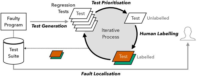
Figure 3. Overview of Iterative Fault Localisation with Test Augmentation

Overview of Iterative Fault Localisation with Test Augmentation

4.2. Iterative Fault Localisation with Test Augmentation

Let us propose an Iterative Fault Localisation (IFL) scenario, in which FDG is used to guide the augmentation of the test suite: an overview of the proposed scenario is presented in Fig. 3.

First, an automated test generation tool, such as EvoSuite (Fraser and Arcuri, 2011) or Randoop (Pacheco and Ernst, 2007), produces regression tests for the given faulty program (Test Generation): to reduce the number of generated test cases, we limit the scope of regression test generation only to the program elements covered by the initial failing test cases. Since regression tests simply capture and record the current behaviour of the program, some assertions in the generated tests may capture the buggy behaviour of the program (Pastore et al., 2013). Note that the regression test cases generated by EvoSuite always capture the behaviour of the current system as identity assertions (Fraser and Zeller, 2012). Fig. 4 shows an example of a test case automatically generated for the Defects4J Math-59 buggy version by EvoSuite: when calling FastMath.max(0.0F, (-1653.0F)) (Line 3), the assertion generated from the buggy program expects the return value to be -1653.0F (Line 4), and not 0.0F, which is the buggy behaviour of Math-59.

⬇

1 @Test(timeout = 4000)

2 public void test03() throws Throwable {

3 float f0 = FastMath.max(0.0F, (-1653.0F));

4 // wrong assertion! (f0 should be 0.0F)

5 assertEquals((-1653.0F), f0, 0.01F);

6 }

Figure 4. An EvoSuite-generated test case for the class FastMath of Math-59 in Defects4J

An EvoSuite-generated test case for the class FastMath of Math-59 in Defects4J

Consequently, unless the failure is detectable by implicit oracles (Barr et al., 2015) such as program crashes or uncaught exceptions, a human engineer has to determine whether the program behaviour captured in the test case is correct or incorrect (Human Labelling, or Oracle Elicitation). For example, an engineer will say that the test case in Fig. 4 is capturing the incorrect behaviour. However, since manual oracle elicitation can be costly, tests should be presented to the engineer in the order of their relative diagnostic capabilities so that the more relevant tests to the fault localisation are labelled earlier. Therefore, at each iteration, all remaining test cases in the generated test suite are prioritised based on their diagnosability gain, and the best one is selected to be labelled by the engineer. (Test Prioritisation). Note that the only cost not shown in Fig. 3 is that of measuring the coverage of generated tests, which we expect to be automatable for EvoSuite generated tests.

Input: Faulty program $P$, Initial test suite $T$, Test results $R$, Test generation tool TestGenerator, SBFL formula FaultLocaliser, Diagnostic capability metric $f$, Test generation time budget $b_{t}$, Querying budget $b_{q}$

Precondition: $\exists t\in T.R(t)=0$

Output: Fault localisation result

1 $P_{susp}\leftarrow\textsc{GetSuspiciousParts}(T,R)$

2 $T^{\prime}\leftarrow\textsc{TestGenerator}(P_{susp},b_{t})$

3 $i\leftarrow 1$

4 while $i\leq b_{q}\land T^{\prime}\neq\emptyset$ do

       $t_{s}\leftarrow\operatorname*{argmax}_{t\in T^{\prime}}f(T,t)$

        // select $t_{s}$ from $T^{\prime}$

       $R(t_{s})\leftarrow\textsc{GetHumanLabel}(t_{s})$

        // label $t_{s}$

       $T\leftarrow T\cup\{t_{s}\}$

        // add $t_{s}$ to $T$

       $T^{\prime}\leftarrow T^{\prime}\setminus\{t_{s}\}$

        // remove $t_{s}$ from $T^{\prime}$

5       $i\leftarrow i+1$

6      

7 end while

return $\textsc{FaultLocaliser}(T,R)$

Algorithm 1 Iterative FL with Test Augmentation

Algorithm 1 formally describes the workflow. The test generation tool, TestGenerator, generates tests $T^{\prime}$ for the suspicious part $P_{susp}$ of a given faulty program $P$ within the time budget $b_{t}$ (Line 1-2). Then, until either the oracle querying budget, $b_{q}$, is exhausted or $T^{\prime}$ becomes empty, a test case $t_{s}$ with the maximum diagnosability value is iteratively selected from from $T^{\prime}$ (Line 4-5). If the test $t_{s}$ reveals buggy behaviour of a program, the user labels it as Incorrect (i.e., $R(t_{s})=0$), or otherwise as Correct (i.e., $R(t_{s})=1$) (Line 6). Once labelled, the test is moved from $T^{\prime}$ to $T$ (Line 7-8). Finally, after the loop terminates, the final FL result is returned (Line 11).

5. Experimental Setup

This section presents the research questions and describes the setup and the environment of our empirical evaluation.

5.1. Research Questions

We ask the following research questions to evaluate both our newly proposed diagnosability gain metric, FDG, and our IFL approach.

5.1.1. RQ1. Effectiveness

How effective is FDG when compared to the existing metrics? To answer RQ1, we use the same evaluation protocol used for existing metrics, and compare the results produced by FDG to those produced by existing metrics. RQ1 is designed to investigate the performance of FDG in an ideal situation with the perfect knowledge of coverage of all test cases as well as human-written test oracles. While some of the assumptions may be infeasible in practice, we aim to establish the upper bound of FDG in an ideal setting, as a baseline to our subsequent evaluation of IFL scenario. We set $\alpha$ to 0.5 for FDG.

In addition to mAP, we also report the Top-n Accuracy (acc@n), a widely-adopted measure of fault localisation performance. For all faulty subjects, acc@n counts the number of subjects where at least one of the faulty program elements are ranked within the top $n$ locations. As in mAP, we report acc@n after each iteration using the test cases chosen up to that point. When there are multiple test orderings for a single Defects4J bug due to multiple failing test cases (see Section 3.2.1), we average all relevant acc@n values.

5.1.2. RQ2. IFL Performance

How effectively does FDG facilitate fault localisation by prioritising automatically generated test cases? RQ2 aims to investigate the performance of FDG when used in the IFL scenario described in Section 4.2. We conduct IFL as shown in Algorithm 1, starting with an initial test suite, $T$, which contains only the Defects4J-provided failing test cases. Our IFL scenario for RQ2 consists of the following elements:

Test Generation: We employ EvoSuite (Fraser and Arcuri, 2011) version 1.0.7 as a test data generation tool. The target of regression test generation is restricted to only the methods covered by initial failing test cases, as specified in the property relevant.classes in Defects4J. We use two time budgets ($b_{t}$), 3 and 10 minutes, and allocate the physical time budget to a class proportionally to the number of suspicious methods in the class. For example, consider suspicious classes A and B that contain five and ten suspicious methods, respectively. Under the 3-minute budget, we allocate 1 and 2 minutes to class A and B, respectively. We generate 10 test suites for each fault and time budget to cater for the randomness of EvoSuite.

Coverage & FL: We measure the coverage achieved by generated test cases against all suspicious classes using Cobertura. We perform method level SBFL using Ochiai as described in Section 3.2.1.

Test Prioritisation: FDG (with $\alpha=0.5$) is used as the test prioritisation metric $f$ in Line 5 of Algorithm 1.

Human Labelling: We simulate a perfect human oracle querying by running the generated test cases on the fixed version. If a regression test case fails on the fixed version (due to oracle violation or compile error), we consider the test as a failing test case for the buggy version. We report results from $\{1,3,5,10\}$ iterations by setting the oracle querying budget, $b_{q}$, accordingly.

5.1.3. RQ3. Robustness

How robust is FDG against human errors, when used to guide oracle querying? Our third research question concerns the assumption of the perfect human oracle because, in reality, the human engineer may make incorrect judgements about the generated oracles that capture the current behaviour of a buggy program. To study how robust our IFL scenario is against such mistakes, we simulate labelling errors by applying the probability $p\in\left\{0.1,0.3,0.5,0.7,0.9\right\}$ of flipping the perfect judgement, and observe how much the localisation performance deteriorates.

5.1.4. RQ4. Parameter Tuning

What is the ideal parameter $\alpha$ for FDG? FDG has a parameter $\alpha$ that adjusts the relative weights of Split and Cover. For previous research questions, $\alpha$ has been set to 0.5 to assume equal contribution from Split and Cover to the measure of diagnosability gain and, consequently, to the prioritisation. Our final research question studies the impact of the parameter $\alpha$ on the performance of FDG. To answer RQ4, we perform a grid search for $\alpha\in\{0.1,0.3,0.5,0.7,0.9\}$ to find its value that leads to the best prioritisation performance for EvoSuite-generated tests.

Table 1. Experimental Subject - Defects4J

Subject	# Faults	kLoC	Avg. # Tests		Avg. # Methods
			Total	Failing	Total	Suspi cious	Faulty
Commons-lang	65	22	1,527	1.9	2,245	14.7	1.5
Commons-math	106	85	2,713	1.7	3,602	53.2	1.7
JFreeChart	26	96	4,903	3.5	2,205	127.5	4.5
Joda-Time	27	28	1,946	2.8	4,130	375.4	2.0
Closure compiler	133	90	5,038	2.6	7,927	855.4	1.8
Total	357

5.2. Subject

Our empirical evaluation considers 357 faults in five different projects provided by Defects4J version 2.0.0 (Just et al., 2014), a real-world fault benchmark of Java programs. Each fault in Defects4J is in the program source code, not in the configuration nor test files, and the corresponding patch is provided as a fixing commit. For each faulty program, human-written test cases, at least one of which is bound to fail due to the fault, are provided. The failing tests all pass once the fixing commit is applied to the faulty version. Table 1 shows the statistics of our subjects. The Suspicious column contains the average number of methods covered by at least one failing test.

For RQ1, we exclude a total of six faults from the 357 in Table 1: two omission faults, Lang-23 and Lang-56, as they cannot be localised within the faulty version by SBFL techniques, as well as four deprecated faults (Lang-2, Time-21, Closure-63, and Closure-93).

For RQ2 to RQ4, we exclude two additional faults, Time-5 and Closure-105, because the Defects4J-provided lists of relevant (suspicious) classes of those faults do not contain the actual faulty class due to an unknown reason. Overall, 349 faults are used, with 2.3 failing test cases on average per fault in the initial test suites.

5.3. Implementation & Environment

All our experiment have been performed on machines equipped with Intel Core i7-7700 CPU and 32GB memory, running Ubuntu 16.04. We use Java 8 for EvoSuite and Cobertura. Our replication package, available online at https://github.com/agb94/FDG-artifact (An, 2022), includes all implementation as well as the data required to reproduce our work.

6. Results

This section presents the answers to our research questions based on the results of our empirical evaluations.

Table 2. The acc@n values with the selected human-written test cases of Defects4J at each iteration (# total subjects = 351)

		acc
		@1	@3	@5	@10	@1	@3	@5	@10	@1	@3	@5	@10	@1	@3	@5	@10	@1	@3	@5	@10	@1	@3	@5	@10
Metric		EntBug (mAP=0.119)				Total (mAP=0.119)				DDU (mAP=0.149)				Add. (mAP=0.158)				RAPTER (mAP=0.158)				TfD (mAP=0.208)
Iter.	Init.	4	30	45	65	4	30	45	65	4	30	45	65	4	30	45	65	4	30	45	65	4	30	45	65
	1	9	40	61	80	9	40	61	80	10	43	64	85	9	39	60	80	9	39	60	80	21	51	67	84
	2	9	41	63	85	9	41	63	85	12	49	74	99	10	44	67	94	10	44	67	94	28	67	81	100
	3	9	40	64	90	9	40	64	90	14	53	76	107	11	47	71	99	12	48	72	100	32	71	88	112
	4	9	40	64	94	9	40	64	94	15	54	77	112	12	52	76	104	13	53	76	104	33	81	95	127
	5	9	41	67	95	9	41	67	95	15	54	79	115	12	54	80	112	13	53	81	112	35	82	98	130
	6	9	41	67	96	9	41	67	96	15	55	79	118	14	56	82	115	16	56	83	117	35	87	100	134
	7	9	41	68	96	9	41	68	96	15	56	81	123	15	57	85	119	16	57	84	117	36	89	105	142
	8	9	41	68	99	9	41	68	99	15	56	81	125	17	60	86	121	18	59	85	123	37	89	109	145
	9	11	43	68	99	11	43	68	99	16	58	82	127	19	62	87	125	20	61	87	126	37	91	111	149
	10	12	44	68	101	12	44	68	101	17	59	84	127	19	65	88	127	20	63	87	127	39	93	111	149
	Full	110	208	250	277	110	208	250	277	110	208	250	277	110	208	250	277	110	208	250	277	110	208	250	277
Metric		FLINT (mAP=0.113)				Prox (mAP=0.250)				S3 (mAP=0.271)				Split (mAP=0.277)				Cover (mAP=0.278)				FDG (mAP=0.298)
Iter.	Init.	4	30	45	65	4	30	45	65	4	30	45	65	4	30	45	65	4	30	45	65	4	30	45	65
	1	4	31	47	69	27	71	97	130	22	51	69	92	22	51	69	92	25	75	94	122	24	64	87	109
	2	8	45	66	79	34	87	118	145	32	70	93	124	31	70	92	121	35	93	113	145	41	100	124	155
	3	8	47	68	79	40	97	122	158	40	88	108	137	40	91	112	146	46	105	130	164	48	107	135	175
	4	8	48	69	81	42	107	130	168	47	97	124	151	46	106	126	153	53	114	145	181	52	115	145	190
	5	8	48	70	82	45	109	137	174	54	105	128	158	52	114	135	160	54	121	154	188	57	121	158	204
	6	9	49	72	83	47	112	140	182	56	113	135	160	59	122	141	164	55	128	155	192	60	130	164	212
	7	9	49	72	86	47	115	144	185	63	118	141	164	60	125	144	171	57	131	162	198	64	135	170	221
	8	9	50	73	86	48	120	153	188	66	120	146	171	62	129	151	176	61	133	167	204	65	139	174	219
	9	11	52	75	86	49	122	155	190	66	124	149	179	64	130	153	178	62	133	175	209	66	145	178	220
	10	11	52	75	86	50	125	160	195	70	127	153	180	68	134	157	189	63	139	170	212	68	148	179	222
	Full	110	208	250	277	110	208	250	277	110	208	250	277	110	208	250	277	110	208	250	277	110	208	250	277

6.1. RQ1: Effectiveness

Table 2 shows the localisation performance of each metric on Defects4J human-written tests. Each row presents acc@n values ($n\in[1,3,5,10]$) of SBFL results at each iteration; rows Init. and Full represent the results when using a single initial failing test case and full test suite (about 4.2K tests on average), respectively. The numbers in bold represent the highest values in the iteration for the corresponding $n$ value. Additionally, the mAP values after ten iterations are shown next to the name of each metric.

The results show that FDG outperforms all nine studied metrics by achieving the highest acc@3, 5, 10 values in all iterations except for the first. Especially at the tenth iteration, acc@10 is 23% and 14% higher than those obtained by the state-of-the-art metrics, S3 and Prox, respectively. Furthermore, we report the performance of Split and Cover as stand-alone metrics. Although they do not perform as well as FDG, the two subcomponents still achieve higher mAP values than all existing metrics after ten iterations, showing each of them can outperform the existing metrics as a stand-alone diagnosability metric.

Additionally, we also compare the FL accuracy at the tenth iteration to the accuracy obtained using the initial test set only, as well as the full test suites. After adding ten test cases based on FDG, acc@1 and acc@10 values are increased by 17.0 and 3.4 times, respectively, compared to the initial test set. Notably, FDG achieves $62\%$ of acc@1 and $80\%$ of acc@10 compared to the full test suite, after ten iterations, despite the fact that the full test suites have approximately 380 times (=4.2K/11) more tests than the 11 test cases obtained using FDG (one initial + ten additional).

6.2. RQ2: IFL Performance

Table 3. Average number of tests generated by EvoSuite (number of failing tests in parenthesis)

Time	Project
Budget	Lang	Math	Chart	Time	Closure
3 mins	32 (1.0)	97 (0.8)	225 (2.4)	442 (0.7)	832 (0.2)
10 mins	34 (1.1)	102 (0.9)	233 (2.5)	475 (0.8)	964 (0.4)

Table 3 shows the average number of total and failing test cases generated by EvoSuite for the studied faults, using 3 and 10 minutes as time budgets, $b_{t}$, respectively (hereafter denoted by T3 and T10). These tests correspond to $T^{\prime}$ in Algorithm 1. Using these generated test cases, we evaluate fault localisation performance after a different number of oracle queries.

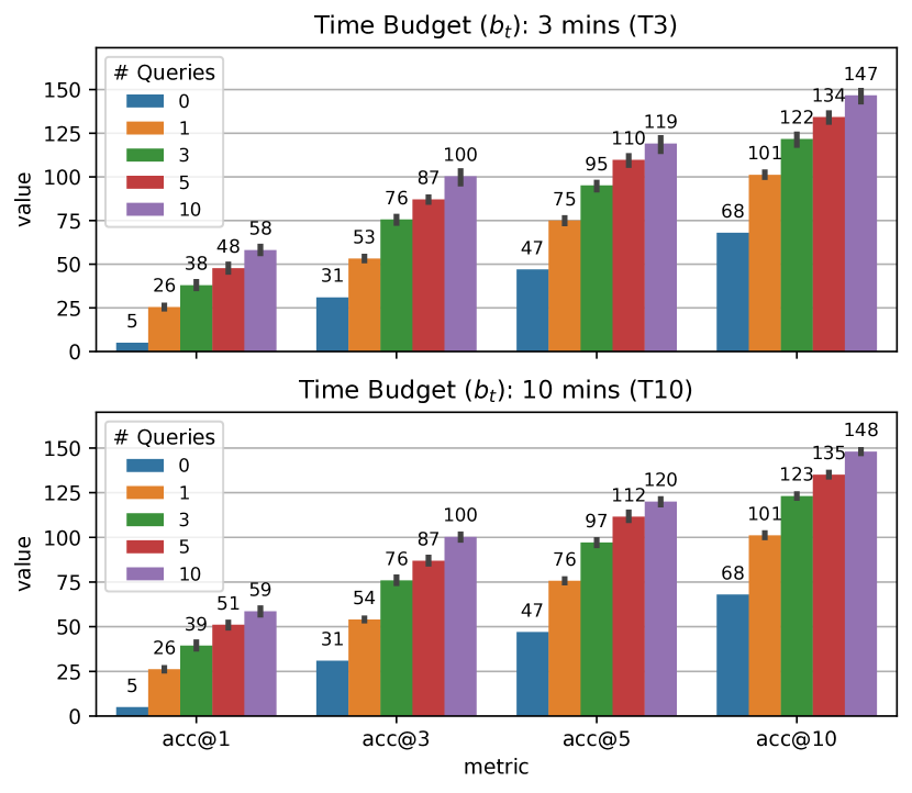
Figure 5. The acc@n values for each time and query budgets. The error bars show the standard error from different seeds. (# total subjects = 349)

Fig. 5 shows how the acc@n values change as the query budget increases for T3 (top) and T10 (bottom) scenarios. Overall, T10 has slightly better localisation results and less standard deviation in performance than T3, although the difference is not significant. This is as expected, for T10 is larger, thus more likely to contain diverse test cases. We note that the effectiveness of test suite augmentation with automatically generated test cases is less than that of augmentation with human-written test cases. However, augmenting the test suite with generated test cases also increases the SBFL accuracy significantly. The test suite with ten newly labelled test cases achieves 11.6x acc@1 ($=58/5$) and 2.2x acc@10 ($=147/68$) compared to those of the initial test suite (# queries = 0).

Interestingly, we note that accurate fault localisation does not always require many additional failing test cases to be generated. The localisation results tend to be positive despite the small number of failing test cases that have been generated (see Table 3). This is because generated passing test cases can still effectively contribute to decreasing the suspiciousness of non-faulty program elements.

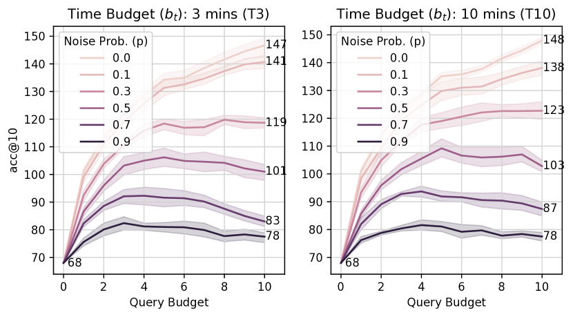
The acc@10 values for each labelling error rate and query budget. Each band shows the standard error of the observations from different seeds.

Figure 6. The acc@10 values for each labelling error rate and query budget. Each band shows the standard error of the observations from different seeds.

6.3. RQ3: Robustness

Fig. 6 shows how localisation performance varies against different labelling error rates. The results show that localisation performance, acc@10, gradually deteriorates as the error rate ($p$) increases. However, we observe that the localisation results are fairly robust up to the error rate of $p=0.3$: the acc@10 values still increase as the query budget increases. Based on the report from Pastore et al. (Pastore et al., 2013) that shows a qualified crowd can achieve accuracy above 0.69 when classifying incorrect assertions for EvoSuite-generated test cases, the error rate tolerance of up to 0.3 shows the robustness of FDG.

Overall, the results show that, despite some errors in labelling, adding new test cases significantly increases the SBFL accuracy compared to the initial test suite. This is because the correctly labelled subsequent test cases can mitigate the impact of earlier labelling errors. Further, we observe that T10 is slightly more robust than T3 against the same error rate. This suggests that the richer the generated test suite is, the more likely it contains tests that can adjust the errors caused by the incorrect labels.

6.4. RQ4: Parameter Tuning

Table 4 shows the performance of FDG obtained while varying $\alpha$ from 0.1 to 0.9 with the interval of 0.2: a value higher than 0.5 means that FDG puts more emphasis on Split, while lower than 0.5 puts more emphasis on Cover. When only one query is made, FL performance measured using acc@10 is best at $\alpha=0.5$. However, as more queries are made, the higher $\alpha$ values, e.g. 0.7, 0.9, or 1.0, tend to produce better performance. These results show that it is better to balance the weights of two metrics ($\alpha$ = 0.5) when the query budget is low, whereas it is better to focus on splitting the ambiguity groups ($\alpha>0.5$) when there are multiple chances to query test oracles from developers. Since both program structure and test suite composition can significantly affect the ambiguity groups, we suggest that $\alpha$ needs to be tuned based on actual fault data when used in practice. However, the results also show that FDG can outperform state-of-the-art diagnosability metrics even with the default value of $\alpha=0.5$.

Table 4. The averaged acc@10 values for T10 test suites

Diagnosability Metric	# Queries
	0	1	3	5	10
FDG ($\alpha=0.0$) = Cover	68	98.4	121.2	131.4	144.0
FDG ($\alpha=0.1$)	68	98.7	122.1	131.8	144.9
FDG ($\alpha=0.3$)	68	98.7	125.3	135.9	146.6
FDG ($\alpha=0.5$)	68	101.1	123.1	135.1	148.0
FDG ($\alpha=0.7$)	68	98.1	126.1	135.9	148.7
FDG ($\alpha=0.9$)	68	93.3	125.7	135.3	151.7
FDG ($\alpha=1.0$) = Split	68	91.8	120.7	139.8	151.0
Prox	68	99.5	119.7	126.6	137.8
S3	68	91.8	117.3	133.9	146.3

7. Discussion

We discuss some assumptions and implications related to FDG.

7.1. Rankings and FL

Whether reporting in the form of linear rankings is the best vessel for fault localisation remains under debate: Parnin and Orso state that human developers do not really follow a given ranking linearly while debugging (Parnin and Orso, 2011), while Xia et al. state that they do help, especially if they are of high quality (Xia et al., 2016). In this work, we simply adopt the ranking based evaluation as one possible way of quantitatively measuring the diagnosability gain.

Note that higher SBFL rankings mean more diverse patterns and fewer ambiguity groups in the achieved coverage, both of which contribute to the general diagnosability of a test suite. In fact, it is entirely possible that the human labelling phase (see Section 4.2) can be the debugging activity itself, as the labeller will have to consider program behaviour and test results for the given task. However, even in such a scenario, we expect that FDG will still prioritise test results efficiently for the labeller. Such a human study would be a very interesting future work.

7.2. Retaining Generated Test Cases

The test suite augmentation scenario proposed in Section 4.2 assumes that 1) there is no other test case apart from the failing test cases, and 2) the new test cases are generated for the purpose of FL only. What if there already exists a test suite, but the newly generated test cases can further improve its diagnosability? The generated test cases do not have to be single-use only: once labelled, selected test cases can be retained to be part of the existing test suites, as long as the testing budget can afford them.

7.3. FDG as Test Generation Objective

Instead of prioritising already generated test cases using FDG, it may also be possible to use to directly adopt FDG as a fitness (or an objective) function that guides test case generation. Note that FDG itself can be considered as a weighted-sum of Cover and Split, which will try to achieve coverage and break ambiguity groups, respectively. As such, we expect that search-based test data generation guided by FDG may yield test suites with high coverage and high diagnosability.

8. Related Work

We have discussed existing work on diagnosability metrics for test cases in Section 3.1. This section further discusses fault localisation techniques that involve human-in-the-loop, as well as a test suite augmentation for fault localisation and algorithmic debugging, which are related to our IFL scenario in Section 4.2.

8.1. Human-in-the-Loop Debugging

Many debugging techniques depend on user feedback. Types of required feedback include the correctness of a specific program element (Bandyopadhyay and Ghosh, 2012; Gong et al., 2012), the correctness of a specific variable value (Lin et al., 2017), the correctness of a specific execution (Li et al., 2016), and the relative location of the fault with respect to breakpoints (Hao et al., 2009a); some techniques provide visual feedback (Hao et al., 2009b; Ko and Myers, 2004, 2008). FDG requires the user to check the automatically generated test assertions, which is similar to checking the correctness of executions (Li et al., 2016). However, the main contribution of FDG lies in the way it chooses which test to get the feedback about. ENLIGHTEN (Li et al., 2018) asks the developer to investigate input-output pairs of the most suspicious method invocations: the feedback is then encoded as a virtual test and used to update the localisation results. Recently, Böhme et al. proposed Learn2Fix (Böhme et al., 2019), a human-in-the-loop program repair technique. Learn2Fix generates test cases by mutating the failing test and allowing the user to label them in the order of their likelihood of failing. Learn2Fix trains an automatic bug oracle using user feedback, which is in turn used to amplify the test suite for better patch generation. While our iterative localisation scenario also requires human interaction, the scenario differs from existing techniques in that it only requires judgements on the correctness of automatically generated assertions.

8.2. Test Augmentation for Fault Localisation

Automated test generation has been widely used to support fault localisation by augmenting insufficient test suites. Artzi et al. (Artzi et al., 2010) used dynamic symbolic execution to generate test cases that are similar to failing executions (Renieres and Reiss, 2003). This type of methodology also can be plugged into the part of our debugging scenario as a test generation tool. BUGEX (Rö$\beta$ler et al., 2012) generates additional test cases similar to a given failing one using EvoSuite and uses an automated oracle to differentiate between passing and failing executions. Finally, BUGEX identifies the runtime properties that are relevant to the failure by comparing passing and failing executions. Compared to BUGEX, our debugging scenario does not assume the existence of an automated bug oracle and instead uses test prioritisation to reduce the cost of querying oracles from a developer. $F^{3}$ (Jin and Orso, 2013) is a fault localisation technique for field failures, which extends a bug reproduction technique, BugRedux (Jin and Orso, 2012): it synthesises failing and passing executions similar to the field failure and uses them for its customised fault localisation technique. While $F^{3}$ can only debug program crashes that can be detected implicitly, our scenario aims to localise faults where no such automatic oracle is available.

Xuan et al. (Xuan and Monperrus, 2014) split test cases into smaller test cases to increase the fault diagnosability of the given test suite. In comparison, we consider cases in which only a few failing test cases are available and use an automated test data generation technique to support fault localisation. Recently, Kuma et al. (Kuma et al., 2020) presented several strategies for selecting the minimum number of test cases out of many automatically generated test cases. However, they only focus on differences in a program spectrum and do not quantify the diagnosability of test cases, which is why we exclude this work from our analysis. Moreover, Kuma et al. use the behaviour of the past version as the test oracle, which may limit its applicability due to limited access to the past versions or version compatibility issues.

8.3. Algorithmic Debugging

Algorithmic debugging (Caballero et al., 2017) was first proposed by Shapiro (Shapiro, 1982) for logic programming languages such as PROLOG. Shapiro introduces an approach that can systemically narrow down the cause of incorrect computation using what is called a debugging tree, whose root node corresponds to the final outcome of the computation, while each subtree represents an intermediate computation whose result is used to compute its parent node. The debugger can systematically guide the user through the debugging tree, narrowing down the possible root cause of the incorrect computation. FDG shares a few similarities with algorithmic debugging: the user is expected to judge the correctness of the final computation (i.e., the test oracle), and the technique tries to systematically narrow down the root cause by breaking ambiguity groups. However, FDG does not require the user to make any judgement about any target program elements, allowing anyone who understands the input-output specification to use it.

9. Threats to Validity

Threats to internal validity regard factors that may influence the observed effects, such as the integrity of the coverage and test results data, as well as the test data generation and fault localisation. To mitigate such threats, we have used the widely studied Cobertura and EvoSuite, as well as the publicly available scripts in Defects4J, to collect or generate data.

Threats to external validity concern any factors that may limit the generalisation of our results. Our results are based on Defects4J, a benchmark against which many fault localisation techniques are evaluated. However, only further experimentations using more diverse subject programs and faults can strengthen the generalisability of our claims. We also consider an iterative scenario, in which tests are chosen and added one by one. It is possible that non-constructive heuristics such as Genetic Algorithm may produce different and potentially better orderings. Our approach is based on the assumption that an iterative process will make it easier for the human engineer to make the oracle judgement.

Finally, threats to construct validity concern situations where used metrics may not reflect the actual properties they claim to measure. All evaluation metrics used in our study are widely used in fault localisation literature, leaving little room for misunderstanding. It is possible that Coincidental Correctness (CC) (Masri et al., 2009) has interfered with our measurements, as it is known to exist in Defects4J (Abou Assi et al., 2019). However, it is theoretically impossible to entirely filter out CC from test results. We also note that all coverage-based fault localisation techniques are equally affected by CC.

10. Conclusion

We propose FDG, a novel measure of the diagnosability of test cases for SBFL. When evaluated with the human-written test cases in Defects4J, FDG can successfully augment single failing test cases, so that adding only ten more test cases improves acc@10 by 3.4 times. The augmentation based on FDG also achieves 23% and 14% higher acc@10 when compared to those based on state-of-the-art metrics, S3 and Prox, respectively. We also introduce an iterative fault localisation scenario, in which the localisation starts with insufficient test suites that contain only failing test cases. By automatically generating test cases using EvoSuite, and prioritising them for human oracle judgements using FDG, we show that acc@1 can be improved by 11.6 times after only ten human interactions. Future work will consider closer integration of FDG and test data generation to improve the overall efficiency of our approach. In particular, we expect that FDG can provide guidance for search based test data generation to improve the the diagnosability of the generated test cases.

References

- (1)
- Abou Assi et al. (2019) Rawad Abou Assi, Chadi Trad, Marwan Maalouf, and Wes Masri. 2019. Coincidental correctness in the Defects4J benchmark. Software Testing, Verification and Reliability 29, 3 (2019), e1696.
- Abreu et al. (2006) Rui Abreu, Peter Zoeteweij, and Arjan JC Van Gemund. 2006. An evaluation of similarity coefficients for software fault localization. In 2006 12th Pacific Rim International Symposium on Dependable Computing (PRDC’06). IEEE, 39–46.
- An (2022) Gabin An. 2022. agb94/FDG-artifact. (May 2022). https://doi.org/10.5281/zenodo.6525227
- Artzi et al. (2010) Shay Artzi, Julian Dolby, Frank Tip, and Marco Pistoia. 2010. Directed test generation for effective fault localization. In Proceedings of the 19th international symposium on Software testing and analysis. 49–60.
- B. Le et al. (2016) Tien-Duy B. Le, David Lo, Claire Le Goues, and Lars Grunske. 2016. A Learning-to-rank Based Fault Localization Approach Using Likely Invariants. In Proceedings of the 25th International Symposium on Software Testing and Analysis (ISSTA 2016). ACM, New York, NY, USA, 177–188.
- Bandyopadhyay and Ghosh (2011) Aritra Bandyopadhyay and Sudipto Ghosh. 2011. Proximity based weighting of test cases to improve spectrum based fault localization. In 2011 26th IEEE/ACM International Conference on Automated Software Engineering (ASE 2011). IEEE, 420–423.
- Bandyopadhyay and Ghosh (2012) Aritra Bandyopadhyay and Sudipto Ghosh. 2012. Tester feedback driven fault localization. In 2012 IEEE Fifth International Conference on Software Testing, Verification and Validation. IEEE, 41–50.
- Barr et al. (2015) Earl Barr, Mark Harman, Phil McMinn, Muzammil Shahbaz, and Shin Yoo. 2015. The Oracle Problem in Software Testing: A Survey. IEEE Transactions on Software Engineering 41, 5 (May 2015), 507–525.
- Baudry et al. (2006) Benoit Baudry, Franck Fleurey, and Yves Le Traon. 2006. Improving test suites for efficient fault localization. In Proceedings of the 28th international conference on Software engineering. 82–91.
- Böhme et al. (2019) Marcel Böhme, Charaka Geethal, and Van-Thuan Pham. 2019. Human-In-The-Loop Automatic Program Repair. arXiv preprint arXiv:1912.07758 (2019).
- Caballero et al. (2017) Rafael Caballero, Adrián Riesco, and Josep Silva. 2017. A Survey of Algorithmic Debugging. ACM Comput. Surv. 50, 4 (aug 2017).
- Campos et al. (2013) José Campos, Rui Abreu, Gordon Fraser, and Marcelo d’Amorim. 2013. Entropy-based test generation for improved fault localization. In 2013 28th IEEE/ACM International Conference on Automated Software Engineering (ASE). IEEE, 257–267.
- Elbaum et al. (2002) Sebastian Elbaum, Alexey G Malishevsky, and Gregg Rothermel. 2002. Test case prioritization: A family of empirical studies. IEEE transactions on software engineering 28, 2 (2002), 159–182.
- Fraser and Arcuri (2011) Gordon Fraser and Andrea Arcuri. 2011. Evosuite: automatic test suite generation for object-oriented software. In Proceedings of the 19th ACM SIGSOFT symposium and the 13th European conference on Foundations of software engineering. 416–419.
- Fraser and Zeller (2012) G. Fraser and A. Zeller. 2012. Mutation-Driven Generation of Unit Tests and Oracles. IEEE Transactions on Software Engineering 38, 2 (2012), 278–292.
- Gong et al. (2012) Liang Gong, David Lo, Lingxiao Jiang, and Hongyu Zhang. 2012. Interactive fault localization leveraging simple user feedback. In 2012 28th IEEE International Conference on Software Maintenance (ICSM). IEEE, 67–76.
- Gonzalez-Sanchez et al. (2011a) Alberto Gonzalez-Sanchez, Rui Abreu, Hans-Gerhard Gross, and Arjan JC van Gemund. 2011a. Prioritizing tests for fault localization through ambiguity group reduction. In 2011 26th IEEE/ACM International Conference on Automated Software Engineering (ASE 2011). IEEE, 83–92.
- Gonzalez-Sanchez et al. (2011b) Alberto Gonzalez-Sanchez, Éric Piel, Rui Abreu, Hans-Gerhard Gross, and Arjan J. C. van Gemund. 2011b. Prioritizing tests for software fault diagnosis. Software: Practice and Experience 41, 10 (2011), 1105–1129. https://doi.org/10.1002/spe.1065
- Gonzalez-Sanchez et al. (2010) Alberto Gonzalez-Sanchez, Eric Piel, Hans-Gerhard Gross, and Arjan JC van Gemund. 2010. Prioritizing tests for software fault localization. In 2010 10th International Conference on Quality Software. IEEE, 42–51.
- Halmos (2017) Paul R Halmos. 2017. Naive set theory. Courier Dover Publications.
- Hao et al. (2010) Dan Hao, Tao Xie, Lu Zhang, Xiaoyin Wang, Jiasu Sun, and Hong Mei. 2010. Test input reduction for result inspection to facilitate fault localization. Automated software engineering 17, 1 (2010), 5.
- Hao et al. (2009a) Dan Hao, Lu Zhang, Tao Xie, Hong Mei, and Jia-Su Sun. 2009a. Interactive fault localization using test information. Journal of Computer Science and Technology 24, 5 (2009), 962–974.
- Hao et al. (2009b) Dan Hao, Lingming Zhang, Lu Zhang, Jiasu Sun, and Hong Mei. 2009b. VIDA: Visual interactive debugging. In 2009 IEEE 31st International Conference on Software Engineering. IEEE, 583–586.
- Hong et al. (2017) Shin Hong, Taehoon Kwak, Byeongcheol Lee, Yiru Jeon, Bongsuk Ko, Yunho Kim, and Moonzoo Kim. 2017. MUSEUM: Debugging Real-World Multilingual Programs Using Mutation Analysis. Information and Software Technology 82 (2017), 80–95.
- Jin and Orso (2012) Wei Jin and Alessandro Orso. 2012. BugRedux: reproducing field failures for in-house debugging. In 2012 34th International Conference on Software Engineering (ICSE). IEEE, 474–484.
- Jin and Orso (2013) Wei Jin and Alessandro Orso. 2013. F3: fault localization for field failures. In Proceedings of the 2013 International Symposium on Software Testing and Analysis. 213–223.
- Jones and Harrold (2005) James A Jones and Mary Jean Harrold. 2005. Empirical evaluation of the tarantula automatic fault-localization technique. In Proceedings of the 20th IEEE/ACM international Conference on Automated software engineering. 273–282.
- Jost (2006) Lou Jost. 2006. Entropy and diversity. Oikos 113, 2 (2006), 363–375.
- Just et al. (2014) René Just, Darioush Jalali, and Michael D Ernst. 2014. Defects4J: A database of existing faults to enable controlled testing studies for Java programs. In Proceedings of the 2014 International Symposium on Software Testing and Analysis. 437–440.
- Ko and Myers (2008) Andrew Ko and Brad Myers. 2008. Debugging reinvented. In 2008 ACM/IEEE 30th International Conference on Software Engineering. IEEE, 301–310.
- Ko and Myers (2004) Andrew J Ko and Brad A Myers. 2004. Designing the whyline: a debugging interface for asking questions about program behavior. In Proceedings of the SIGCHI conference on Human factors in computing systems. 151–158.
- Kuma et al. (2020) Tetsushi Kuma, Yoshiki Higo, Shinsuke Matsumoto, and Shinji Kusumoto. 2020. Improving the Accuracy of Spectrum-based Fault Localization for Automated Program Repair. In Proceedings of the 28th International Conference on Program Comprehension. 376–380.
- Li et al. (2016) Xiangyu Li, Marcelo d’Amorim, and Alessandro Orso. 2016. Iterative user-driven fault localization. In Haifa Verification Conference. Springer, 82–98.
- Li et al. (2019) Xia Li, Wei Li, Yuqun Zhang, and Lingming Zhang. 2019. DeepFL: Integrating Multiple Fault Diagnosis Dimensions for Deep Fault Localization. In Proceedings of the 28th ACM SIGSOFT International Symposium on Software Testing and Analysis (ISSTA 2019). Association for Computing Machinery, New York, NY, USA, 169–180.
- Li et al. (2018) Xiangyu Li, Shaowei Zhu, Marcelo d’Amorim, and Alessandro Orso. 2018. Enlightened debugging. In 2018 IEEE/ACM 40th International Conference on Software Engineering (ICSE). IEEE, 82–92.
- Lin et al. (2017) Yun Lin, Jun Sun, Yinxing Xue, Yang Liu, and Jinsong Dong. 2017. Feedback-based debugging. In 2017 IEEE/ACM 39th International Conference on Software Engineering (ICSE). IEEE, 393–403.
- Masri et al. (2009) Wes Masri, Rawad Abou-Assi, Marwa El-Ghali, and Nour Al-Fatairi. 2009. An empirical study of the factors that reduce the effectiveness of coverage-based fault localization. In Proceedings of the 2nd International Workshop on Defects in Large Software Systems: Held in conjunction with the ACM SIGSOFT International Symposium on Software Testing and Analysis (ISSTA 2009). 1–5.
- Moon et al. (2014) Seokhyeon Moon, Yunho Kim, Moonzoo Kim, and Shin Yoo. 2014. Ask the Mutants: Mutating Faulty Programs for Fault Localization. In Proceedings of the 7th International Conference on Software Testing, Verification and Validation (ICST 2014). 153–162.
- Naish et al. (2011) Lee Naish, Hua Jie Lee, and Kotagiri Ramamohanarao. 2011. A model for spectra-based software diagnosis. ACM Transactions on software engineering and methodology (TOSEM) 20, 3 (2011), 1–32.
- Pacheco and Ernst (2007) Carlos Pacheco and Michael D Ernst. 2007. Randoop: feedback-directed random testing for Java. In Companion to the 22nd ACM SIGPLAN conference on Object-oriented programming systems and applications companion. 815–816.
- Papadakis and Le-Traon (2012) M. Papadakis and Y. Le-Traon. 2012. Using Mutants to Locate ”Unknown” Faults. In Proceedings of the 5th IEEE Fifth International Conference on Software Testing, Verification and Validation (Mutation 2012). 691–700. https://doi.org/10.1109/ICST.2012.159
- Papadakis and Traon (2015) Mike Papadakis and Yves Le Traon. 2015. Metallaxis-FL: mutation-based fault localization. Softw. Test., Verif. Reliab. 25, 5-7 (2015), 605–628. https://doi.org/10.1002/stvr.1509
- Parnin and Orso (2011) Chris Parnin and Alessandro Orso. 2011. Are automated debugging techniques actually helping programmers?. In Proceedings of the 2011 international symposium on software testing and analysis. 199–209.
- Pastore et al. (2013) Fabrizio Pastore, Leonardo Mariani, and Gordon Fraser. 2013. Crowdoracles: Can the crowd solve the oracle problem?. In 2013 IEEE Sixth International Conference on Software Testing, Verification and Validation. IEEE, 342–351.
- Perez et al. (2017) Alexandre Perez, Rui Abreu, and Arie van Deursen. 2017. A test-suite diagnosability metric for spectrum-based fault localization approaches. In 2017 IEEE/ACM 39th International Conference on Software Engineering (ICSE). IEEE, 654–664.
- Renieres and Reiss (2003) Manos Renieres and Steven P Reiss. 2003. Fault localization with nearest neighbor queries. In 18th IEEE International Conference on Automated Software Engineering, 2003. Proceedings. IEEE, 30–39.
- Röler et al. (2012) Jeremias Röler, Gordon Fraser, Andreas Zeller, and Alessandro Orso. 2012. Isolating failure causes through test case generation. In Proceedings of the 2012 international symposium on software testing and analysis. 309–319.
- Rothermel et al. (1999) Gregg Rothermel, Roland H Untch, Chengyun Chu, and Mary Jean Harrold. 1999. Test case prioritization: An empirical study. In Proceedings IEEE International Conference on Software Maintenance-1999 (ICSM’99).’Software Maintenance for Business Change’(Cat. No. 99CB36360). IEEE, 179–188.
- Saha et al. (2013) Ripon K Saha, Matthew Lease, Sarfraz Khurshid, and Dewayne E Perry. 2013. Improving bug localization using structured information retrieval. In Automated Software Engineering (ASE), 2013 IEEE/ACM 28th International Conference on. IEEE, 345–355.
- Shannon (1948) Claude E Shannon. 1948. A mathematical theory of communication. The Bell system technical journal 27, 3 (1948), 379–423.
- Shapiro (1982) Ehud Y. Shapiro. 1982. Algorithmic Program Diagnosis. In Proceedings of the 9th ACM SIGPLAN-SIGACT Symposium on Principles of Programming Languages (POPL ’82). Association for Computing Machinery, New York, NY, USA, 299–308.
- Sohn and Yoo (2017) Jeongju Sohn and Shin Yoo. 2017. FLUCCS: Using Code and Change Metrics to Improve Fault Localisation. In Proceedings of the International Symposium on Software Testing and Analysis (ISSTA 2017). 273–283.
- Stenbakken et al. (1989) GN Stenbakken, TM Souders, and GW Stewart. 1989. Ambiguity groups and testability. IEEE Transactions on Instrumentation and Measurement 38, 5 (1989), 941–947.
- Wong et al. (2014) W. E. Wong, V. Debroy, R. Gao, and Y. Li. 2014. The DStar Method for Effective Software Fault Localization. IEEE Transactions on Reliability 63, 1 (2014), 290–308.
- Wong et al. (2016) W Eric Wong, Ruizhi Gao, Yihao Li, Rui Abreu, and Franz Wotawa. 2016. A survey on software fault localization. IEEE Transactions on Software Engineering 42, 8 (2016), 707–740.
- Xia et al. (2016) X. Xia, L. Bao, D. Lo, and S. Li. 2016. “Automated Debugging Considered Harmful” Considered Harmful: A User Study Revisiting the Usefulness of Spectra-Based Fault Localization Techniques with Professionals Using Real Bugs from Large Systems. In Proceedings of the IEEE International Conference on Software Maintenance and Evolution (ICSME 2016). 267–278.
- Xuan and Monperrus (2014) Jifeng Xuan and Martin Monperrus. 2014. Test case purification for improving fault localization. In Proceedings of the 22nd ACM SIGSOFT International Symposium on Foundations of Software Engineering. 52–63.
- Yoo and Harman (2012) Shin Yoo and Mark Harman. 2012. Regression testing minimization, selection and prioritization: a survey. Software testing, verification and reliability 22, 2 (2012), 67–120.
- Yoo et al. (2013) Shin Yoo, Mark Harman, and David Clark. 2013. Fault localization prioritization: Comparing information-theoretic and coverage-based approaches. ACM Transactions on Software Engineering and Methodology (TOSEM) 22, 3 (2013), 1–29.