GSEIM: A General-purpose Simulator with Explicit and Implicit Methods

Abstract

A new simulation package, GSEIM, for solving a set of ordinary differential equations is presented. The organisation of the program is illustrated with the help of a block diagram. Various features of GSEIM are discussed. Two ways of incorporating new elements in GSEIM, viz., as a template and as a subcircuit, are explained by taking a specific example. Simulation examples are described to bring out the capabilities of GSEIM.

1 Introduction

A wide variety of engineering applications require numerical solution of a set of ordinary differential equations (ODEs), satisfying some given initial conditions. This need is currently addressed by commercial [1],[2] as well as open-source [3] software packages. While the numerical methods for solving ODEs are well-known (see, e.g., [4]-[9]), different packages have different strengths and weaknesses, based on performance, ease of use, capability of adding new library elements, cost, user support, and legacy issues. It is the purpose of this paper to present a new ODE solver called GSEIM (General-purpose Simulator with Explicit and Implicit Methods) and illustrate its working through examples.

The paper is organised as follows. In Sec. 2, we briefly review the advantages and limitations of explicit and implicit methods for solving ODEs. We then describe, in Sec. 3, the block-level organisation of GSEIM. A key feature of GSEIM is the flexibility it gives the user to add new elements to the library. We describe this aspect in Sec. 4 where we point out, using a few examples, how computations related to explicit and implicit methods are incorporated in the element templates. In Sec. 5, we look at how a subcircuit (hierarchical block) can be added to GSEIM, using the example of an induction machine model. One important requirement in many engineering applications is accurate handling of abrupt changes. We describe in Sec. 6 how that is implemented in GSEIM. In Sec. 7, we present two simulations examples to illustrate the capabilities of the new platform. Finally, in Sec. 8, we present our conclusions and comment on future directions.

2 Explicit and implicit methods

There are several well-known explicit and implicit methods for solving ODEs (e.g., see [5]). In order to illustrate the advantage of an explicit method over an implicit method, let us consider a single ODE of the form

$$\frac{dx}{dt}=f(t,x).$$ (1)

The discretised form of this ODE using the improved Euler method (an explicit method) is given by

$$x_{n+1}=x_{n}+\displaystyle\frac{h}{2}\,\left[f(t_{n},x_{n})+f(t_{n}+h,x_{n}+h\,f(t_{n},x_{n}))\right],$$ (2)

where $x_{n}$ and $x_{n+1}$ correspond to the numerical solutions at times $t_{n}$ and $t_{n+1}$, respectively, and $h\,$=$\,t_{n+1}-t_{n}$ is the time step. Since $t_{n}$ and $x_{n}$ are known, computing $x_{n+1}$ involves only evaluation in this case.

Consider now the discretised form of Eq. 1 when the backward Euler method (an implicit method) is used:

$$x_{n+1}=x_{n}+h\,f(t_{n+1},x_{n+1}).$$ (3)

Because $x_{n+1}$ is also involved on the right-hand side, obtaining $x_{n+1}$ in this case requires solution of Eq. 3.

For a system of ODEs, an explicit method would still involve function evaluations, i.e., the process of updating the system variables by evaluating functions of their past values. An implicit method, on the other hand, would give rise to a system of equations which has to be solved. If the system of equations is nonlinear, an iterative procedure such as the Netwon-Raphson method would be required with the associated complication of convergence difficulties. Clearly, from the perspective of work per time step, an explicit method would be advantageous over an implicit method of the same order. However, implicit methods are superior in terms of stability, as illustrated by the following example.

Consider the $RC$ circuit shown in Fig. 1. We are interested in the variation of $V_{1}$ and $V_{2}$ when a step input voltage $V_{s}(t)$ is applied.

Figure 1: $RC$ circuit with two time constants.

For solving the circuit equations numerically, we first rewrite them as a system of ODEs,

$$\begin{array}[]{rl}\displaystyle\frac{dV_{1}}{dt}&=\displaystyle\frac{1}{R_{1}C_{1}}\,(V_{s}-V_{1})-\displaystyle\frac{1}{R_{2}C_{1}}\,(V_{1}-V_{2}),\\ \rule[-9.47217pt]{0.0pt}{0.0pt}\rule{0.0pt}{17.22217pt}\displaystyle\frac{dV_{2}}{dt}&=\displaystyle\frac{1}{R_{2}C_{2}}\,(V_{1}-V_{2}).\end{array}$$ (4)

We expect $V_{1}$ and $V_{2}$ to start changing as the input step is applied and eventually settle down to their steady-state values. For this problem, rather than using constant time steps for the entire interval of interest, it is far more efficient to use small time steps when the variations are rapid and large time steps when they are slow. We consider two methods which employ such adaptive time step computation: (a) the Runge-Kutta-Fehlberg (RKF45) method, an explicit method which employs Runge-Kutta methods of order 4 and 5 in each time step [8], and (b) the TR-BDF2 method, an implicit method, which employs the trapezoidal (TR) and backward difference formula (BDF2) methods in each time step [10].

In each of these methods, an estimate of the local truncation error (LTE) is obtained in each time step. If the LTE is small, the current time step is accepted, and the next time step is allowed to be larger. If the LTE is larger than a specified value, the current time step is rejected, and a smaller time step is tried. As the circuit appraches steady state, the LTE tends to zero, allowing the algorithm to take larger time steps, limited eventually only by an upper limit set by the user.

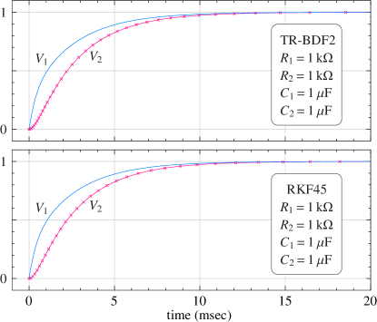
Figure 2: Numerical solution of Eq. 4 using the TR-BDF2 and RKF45 methods. The parameter values are $R_{1}\,$=$\,R_{2}\,$=$\,1$ k$\Omega$, $C_{1}\,$=$\,C_{2}\,$=$\,1\,\mu$F. Crosses show the simulator time points.

Fig. 2 shows the results for $R_{1}\,$=$\,R_{2}\,$=$\,1$ k$\Omega$, $C_{1}\,$=$\,C_{2}\,$=$\,1\,\mu$F. Both RKF45 and TR-BDF2 methods perform as expected. As the circuit approaches steady state, they make the time steps larger, leading to fewer time steps overall and therefore faster simulation.

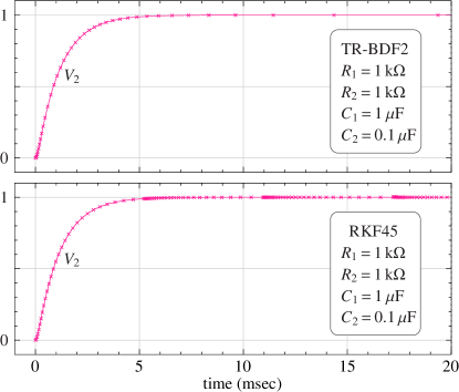
Figure 3: Numerical solution of Eq. 4 using the TR-BDF2 and RKF45 methods. The parameter values are $R_{1}\,$=$\,R_{2}\,$=$\,1$ k$\Omega$, $C_{1}\,$=$\,1\,\mu$F, $C_{2}\,$=$\,0.1\,\mu$F. Crosses show the simulator time points.

When $C_{2}$ is changed from $1\,\mu$F to $0.1\,\mu$F, the two methods show very different behaviour (see Fig. 3). The TR-BDF2 method continues to increase the time step as the circuit approaches steady state. The RKF45 method does increase the time step up to a certain point, but at $t\,$$\approx$$\,5.1$ msec, it forces a small time step. After that, it once again starts increasing the time step, but only up to $t\,$$\approx$$\,10.8$ msec, and so on. This behaviour is related to stability of the RKF45 algorithm. The explicit Runge-Kutta methods employed in the RKF45 algorithm are conditionally stable. They require the time step to be smaller than a certain multiple of the smallest time constant in the system [9]. With $R_{1}\,$=$\,R_{2}\,$=$\,1$ k$\Omega$, $C_{1}\,$=$\,C_{2}\,$=$\,1\,\mu$F, the time constant are $\tau_{1}\,$=$\,2.6$ msec and $\tau_{2}\,$=$\,0.38$ msec. With $C_{2}\,$=$\,0.1\,\mu$F, the time constants are $\tau_{1}\,$=$\,1.1$ msec and $\tau_{2}\,$=$\,0.09$ msec, and the largest time step allowed by the RKF45 algorithm is correspondingly reduced. For the TR-BDF2 method, which is A-stable, there is no such restriction, and therefore it allows large time steps as steady state is approached, thus reducing the computation time significantly.

From the above discussion, it is clear that, from the efficiency perspective, the choice of the method (explicit or implicit) would depend on the problem being solved. For this reason, GSEIM incorporates explicit as well as implicit methods.

3 GSEIM organisation

The block diagram of the GSEIM program is shown in Fig. 4. The schematic entry block (GUI) is adapted from the GNURadio package [11]. It enables the user to prepare a schematic diagram of the system of interest and produces a high-level netlist. A parser program takes the high-level netlist as input, performs parsing of node names and computation of element parameters (if required). As its output, the parser program produces a low-level netlist. The solver takes the low-level netlist as its input, and using information from the library, it prepares and solves the set of ODEs corresponding to the user’s system, creating output files requested by the user. Finally, the plotting program reads the output files and displays the plots in an interactive manner.

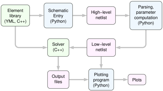
Figure 4: Block diagram of the GSEIM program.

GSEIM has been designed to completely decouple the element library from the solver, which makes it possible for the user to add new elements to the library (if required). For each element (say, xyz), the library contains two files: (a) xyz.xbe which contains information about the variable names, parameter names and values, and equations related to that element, and (b) xyz.yml which specifies how the element would appear in the schematic entry GUI. A detailed description of these files would be presented in the GSEIM manual. In Sec. 4, we will take a brief look at the xbe files for a few elements.

The salient features of the GSEIM package can be described as follows.

• The solver, which handles the most intensive computation, viz., numerical solution of the ODEs, is written in C++ because of its high performance.

• For all other purposes, viz., schematic capture, parsing, parameter computation, and plotting, python is used because of the flexibility and ease of programming it offers.

• Output parameters, which determine what data gets stored in the output files during simulation, are specified without having to add extra elements – such as the “scope” in Simulink [1] and Xcos [3]) – to the schematic diagram. This helps in avoiding clutter.

• Subcircuits (hierarchical blocks) can be used for simplifying the schematic.

• Explicit as well as implicit numerical methods are incorporated in the solver. Currently, the following methods are made available:

  • explicit (fixed time step): improved Euler, Heun, Runge-Kutta (4^th order)

  • explicit (auto time step): RKF45, Bogacki and Shampine (2,3)

  • implicit (fixed time step): backward Euler, trapezoidal

  • implicit (auto time step): backward Euler-auto, trapezoidal-auto, TR-BDF2

  The backward Euler-auto and trapezoidal-auto methods are used only for nonlinear problems. In these methods, the time step is adjusted depending on the number of Newton-Raphson iterations required at a given time point.

• GSEIM provides a GUI for plotting the variables specified by the user. The plotting GUI, shown in Fig. 5, allows the user to select the output file of interest, the $x$-axis variable (typically time), and $y$-axis variable(s) to be included in the plot. It also gives the user control over plot attributes such as line colour, line width, and symbol type, with appropriate values specified by default. Using this information, the plotting GUI displays the plot requested by the user. It also produces python code associated with the plot. If required, the user can edit this code in order to make the plot more suitable for a report or a presentation. This way, the user can benefit from a wide range of plotting capabilities offered by python.

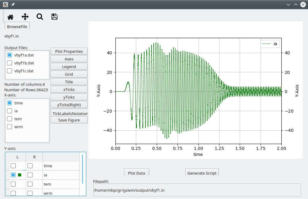
Figure 5: Snapshot of the plotting GUI provided as part of the GSEIM package.

4 Library element templates

A very important feature of GSEIM is that it allows the user to add new functionality in the form of library elements, by writing suitable “templates.” In this section, we look at the syntax of element templates with the help of some examples. We start with a few remarks.

• An element template has three types of variables in general: input, output, and auxiliary. Only the input and output variables are made available in the schematic capture GUI for connection to other elements.

• Two types of elements are allowed:

  • evaluate type in which the element equations are of the form $y\,$=$\,f(x_{1},x_{2},..)$ where $y$ is an output and $x_{1}$, $x_{2}$, etc. are inputs. These elements do not involve time derivatives.

  • integrate type with equations of the form $\displaystyle\frac{dy}{dt}\,$=$\,f(x_{1},x_{2},..)$ where $y$ is an output or auxiliary variable, and $x_{1}$, $x_{2}$, etc. can be input, output, or auxiliary variables.

4.1 Adder

As out first example, we consider the sum_2 element which gives $y\,$=$\,k_{1}x_{1}+k_{2}x_{2}$, where $x_{1}$ and $x_{2}$ are input variables, $y$ is the output variable, and $k_{1}$, $k_{2}$ are real parameters. This is an evaluate type element, i.e., its output can be written as a function of its inputs, and it does not involve time derivatives. Fig. 6 shows the overall structure of sum_2.xbe.

Figure 6: sum_2.xbe template (partial).

The following features may be noted.

• The element name is specified by the keyword name.

• The assignment evaluate=yes specifies the element type.

• The assignment Jacobian: constant indicates that, when the element equation $y-k_{1}x_{1}-k_{2}x_{2}=0$ is differentiated with respect to the variables involved in the equation, we get constants.

• The lines input_vars and output_vars specify the input and output variables of the element, respectively.

• The names and default values of the real parameters are given by the rparms statement. (GSEIM also allows integer and string parameters; they are not used in sum_2.

• The outparms statement specifies the names of output parameters which will be made available by this template for saving to the user’s output files during simulation (if requested by the user).

• The n_f and n_g statements specify the number of $f$ and $g$ functions for this element. (This aspect will be described in detail in the GSEIM manual.)

• The g_1 statement indicates the variables involved in the function $g_{1}$.

• The C++ part of the template, to be described separately, appears between the C and endC statements.

Before we look at the C++ part of sum_2.xbe, let us see where it fits in the overall scheme. The GSEIM library preprocessor embeds the C++ part of each element template in the C++ function corresponding to that element. This function receives objects X and G from the GSEIM main program and is expected to compute various quantities such function values, output parameters, etc. The object G is a global object and is used to pass information about the current time point, type of method being used (implicit or explicit), etc. It also conveys to the element routine, through the flags array, what computation the main program is expecting from the element routine in the present call. The object X is specific to the element being treated, and it contains variables and parameter values related to that element. With this background, we can make the following points about the C++ part of sum_2.xbe, as shown in Fig. 7.

Figure 7: C++ part of the sum_2.xbe template (partial).

• If an explicit method is being used, the template only needs to evaluate y in terms of x1 and x2.

• If an implicit method is being used, the template needs to supply information about the equation it satisfies which in this case is

  $$g_{1}\equiv y-k_{1}x_{1}-k_{2}x_{2}=0.$$ (5)

  If the program is requesting the function value, $g_{1}(x_{1},x_{2},y)$ is evaluated; if it is requesting the derivatives, then $\displaystyle\frac{\partial g_{1}}{\partial x_{1}}$, $\displaystyle\frac{\partial g_{1}}{\partial x_{2}}$, $\displaystyle\frac{\partial g_{1}}{\partial y}$ are evaluated.

• If the program is requesting assignment of output parameters, the parameters listed in the outparms statement (see Fig. 6) are assigned.

4.2 Integrator

Next, we consider an element of type integrate, viz., the integrator which satisfies $y\,$=$\,k\,\int x\,dt$ where $x$ and $y$ are the input and output variables, respectively, and $k$ is a real parameter. Since GSEIM expects the equations to be written in the general form $\displaystyle\frac{dy}{dt}\,$=$\,f(x_{1},x_{2},..)$, we rewrite the integrator equation as $\displaystyle\frac{dy}{dt}\,$=$\,k\,x$. For integrator type elements, we also need to specify the initial or “start-up” value of the state variable(s). For the integrator, we will denote that by $y_{0}$.

Figure 8: integrator.xbe template (partial).

Figure 9: C++ part of the integrator.xbe template (partial).

The integrator template without the C++ part is shown in Fig. 8. The C++ part is shown separately in Fig. 9. The start-up parameter y_st corresponds to $y_{0}$ mentioned above. The fact that time derivative of y is involved in the element equation is indicated by the f_1 statement.

In the C++ part of the template (Fig. 9), we have different sections for start-up and transient simulation. In the start-up section, the equation $y\,$=$\,y_{0}$ is handled. In the transient section, if the method is explicit, only the function $f_{1}\,$=$\,k\,x$ is evaluated; if it is implicit, the function $g_{1}\,$=$\,k\,x$ as well as its derivative $\displaystyle\frac{\partial g_{1}}{\partial x}$ are computed.

4.3 Induction motor

We now look at a more complex element of type integrate, viz., indmc1.xbe, which implements the induction machine model given by,

$$\displaystyle\frac{d{\psi}_{ds}}{dt} = v_{ds}-r_{s}i_{ds},$$ (6)

$$\displaystyle\frac{d{\psi}_{qs}}{dt} = v_{qs}-r_{s}i_{qs},$$ (7)

$$\displaystyle\frac{d{\psi}_{dr}}{dt} = -\,\frac{P}{2}\,\omega_{rm}\psi_{qr}-r_{r}i_{dr},$$ (8)

$$\displaystyle\frac{d{\psi}_{qr}}{dt} = \frac{P}{2}\,\omega_{rm}\psi_{dr}-r_{r}i_{qr},$$ (9)

$$\displaystyle\frac{d{\omega}_{rm}}{dt} = \frac{1}{J}\,(T_{em}-T_{L}),$$ (10)

where

$$i_{ds} = \frac{L_{r}}{L_{m}L_{e}}\,\psi_{ds}-\frac{1}{L_{e}}\,\psi_{dr},$$ (11)

$$i_{qs} = \frac{L_{r}}{L_{m}L_{e}}\,\psi_{qs}-\frac{1}{L_{e}}\,\psi_{qr},$$ (12)

$$i_{dr} = \frac{1}{L_{m}}\,\psi_{ds}-\left(\frac{L_{ls}}{L_{m}}+1\right)~{}i_{ds},$$ (13)

$$i_{qr} = \frac{1}{L_{m}}\,\psi_{qs}-\left(\frac{L_{ls}}{L_{m}}+1\right)~{}i_{qs},$$ (14)

$$T_{em} = \frac{3}{4}\,PL_{m}\,(i_{qs}i_{dr}-i_{ds}i_{qr}),$$ (15)

with $L_{e}\,$=$\,\displaystyle\frac{L_{s}L_{r}}{L_{m}}-L_{m}$, $L_{s}\,$=$\,L_{ls}+L_{m}$, $L_{r}\,$=$\,L_{lr}+L_{m}$.

Figs. 10-13 show the various sections of the indmc1 template. The input variables are $v_{qs}$, $v_{ds}$, $T_{L}$, and the output variable is $\omega_{rm}$. In addition, it has internal (auxiliary) variables $\psi_{ds}$, $\psi_{dr}$, $\psi_{qs}$, $\psi_{qr}$ which are involved in the model equations. The statements f_1, f_2, etc. in Fig. 10 are used to inform the simulator which derivative is involved in that equation. The statements g_1, g_2, etc. are used to indicate which variables are involved in the right-hand side of the corresponding equation.

In the induction machine equations (Eqs. 6-15), there are some “one-time” calculations, e.g., calculation of $L_{e}$, which are not required to be performed in every time step. GSEIM provides a flag for this purpose, as seen in Fig. 11. When this flag is set by the main program, the template computes $L_{e}$ and other one-time parameters, and saves them in the X.rprm vector. Subsequently, these parameters need not be computed again.

The function assignment sections of indmc1.xbe are shown separately in Figs. 12 and 13 for explicit and implicit methods, respectively. In the explicit case (Fig. 12), the function $f_{1}$ (i.e., f[nf_1]) is computed as per the right-hand side of Eq. 6, and so on. In the implicit case (Fig. 13), the function $g_{1}$ is simlarly computed. However, in this case, the derivatives of $g_{1}$ with respect to each of the variables involved in this equation also need to be computed.

As seen from the above example, writing a new template, particularly the Jacobian assignment part, requires some systematic effort. For this reason, some simulation packages allow the use of hardware description languages such as Openmodelica [12] and Verilog-AMS [13], which require from the user only functions in symbolic form. The derivatives are then computed internally by the simulator.

While the “low-level” approach used in GSEIM demands more effort from the user in developing new element templates, it does offer more flexibility – the user is not constrained by the limitations of a high-level language. Furthermore, library development is a one-time activity; once an element template is developed and tested, no further coding is required. We believe therefore that our low-level approach has significant practical relevance.

Figure 10: indmc1.xbe template (partial).

Figure 11: One-time parameter section of indmc1.xbe.

Figure 12: Function evaluation in indmc1.xbe for explicit methods.

Figure 13: Function evaluation in indmc1.xbe for implicit methods.

5 Subcircuits

In many situations, the system of interest is hierarchical in nature, and building it in a modular fashion is easier or more convenient than assembling all the basic blocks at one level. Like simulation packages such as SPICE [14], Simulink [1], Dymola [2], GSEIM also allows hierarchical system building. In this section, we consider the induction machine model of Sec. 4 and describe how it can be implemented as a “subcircuit” (a hierarchical block) rather than writing an element template. For this purpose, we rewrite Eqs. 6-15 such that each of them can be implemented using basic blocks such as adder, multiplier, integrator, etc.

As an example, Eq. 8 can be rewritten as,

$$\psi_{dr}=\int\left(-\,\frac{P}{2}\,\omega_{rm}\psi_{qr}-r_{r}i_{dr}\right)\,dt,$$ (16)

which can be implemented using a multiplier (to multiply $\omega_{rm}$ and $\psi_{qr}$), and the sum_2 and integrator elements described in Sec. 4. Treating Eqs. 6-10 in this manner, we obtain the subciruit shown in Fig. 15.

The following additional points about the implementation may be noted:

• “Virtual” sources and sinks (shown in light yellow colour) are used in order to make wiring less cumbersome. For example, note the virtual sink marked “>idr” and the virtual source marked “idr>”, the two corresponding to the same node.

• Input and output pads (shown in light green colour) are used to indicate the input and output ports the subcircuit symbol will have when it is invoked (from a higher level). For the induction machine subcircuit, vds, vqs, tl are the input ports, and wrm is the output port.

• The subcircuit has the following parameters (not shown in Fig. 15): j, llr, lls, lm, poles, rr, rs, which correspond to $J$, $L_{lr}$, $L_{ls}$, $L_{m}$, $P$, $r_{r}$, $r_{s}$, respectively, in Eqs. 6-10. In implementing the equations, we need to compute quantities which depend on these parameters. For example, consider Eq. 11 for $i_{ds}$, implemented using the sum_2 element marked as s6 in the figure. This element gives $i_{ds}\,$=$\,k_{1}\psi_{ds}+k_{2}\psi_{dr}$, which requires $k_{1}\,$=$\,\displaystyle\frac{L_{r}}{L_{m}L_{e}}$, $k_{2}\,$=$\,-\,\displaystyle\frac{1}{L_{e}}$ to be assigned. For all such assignments, the user is expected to supply a python function specific to the concerned subcircuit. For the induction machine subcircuit (s_indmc), the python block is shown in Fig. 14. The calculations for $k_{1}$ and $k_{2}$ of s6 are shown specifically in the figure. Similarly, several other quantities are computed and stored in the python dictionary received by the s_indmc_parm function as an argument. With this mechanism, the user has significant flexibility in implementing element equations.

  

  Figure 14: Parameter computation for the induction machine subcircuit.

• The user can define “output parameters” for a subcircuit and use those at higher levels, as described in [15]. The output parameters can be mapped to nodes within the subcircuit or to the output parameters of the blocks involved in the subcircuit. These features provide a mechanism for viewing various quantities of interest at different levels when the system is simulated.

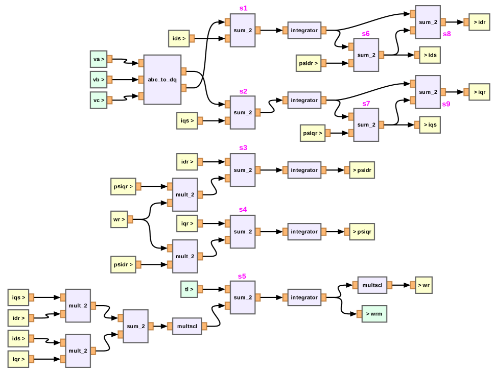
Figure 15: Subcircuit for the induction machine model given by Eqs. 6-15.

6 Handling abrupt changes

In many systems of practical interest, some of the variables are expected to vary abruptly. If the abrupt transitions are missed out by the simulator, it would affect the appearance of the plots of those variables, and more importantly, the accuracy of the simulation results in some cases. As an example, consider a triangle source with period $T\,$=$\,2$ s. If a constant time step $\Delta t\,$=$\,0.12$ s is used, some of the peak or valley points are missed out by the simulator, as seen in Fig. 16 (a). This situation can be improved by tracking the time points where the source output is going to reach a peak or a valley. For this purpose, the triangle source template in GSEIM takes the current time point from the simulator and returns the time of the next “break” (peak or valley). Using this information, GSEIM decides whether the normal time step or a reduced time step should be used next time. Fig. 16 (b) shows the triangle source waveform obtained with this approach.

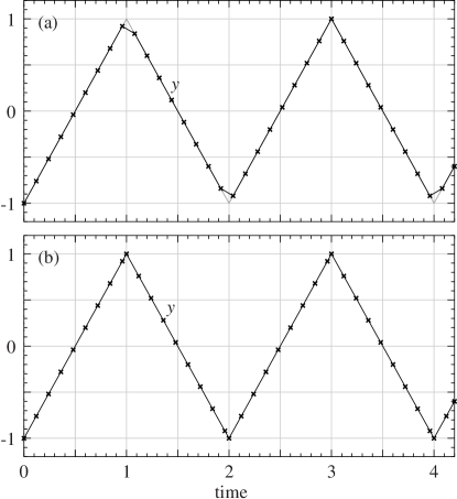
Figure 16: Triangle source waveform: (a) with a constant time step, (b) with time step adjusted for tracking abrupt changes. Crosses show the simulator time points.

Next, consider a comparator with inputs $x_{1}$, $x_{2}$ and output $y$. Fig. 17 (a) shows the $x_{1}$, $x_{2}$, and $y$ waveforms when a constant time step is used. Abrupt changes in $x_{2}(t)$ are tracked by the simulator (as discussed above); however, $y(t)$ is not resolved correctly by the simulator, e.g., see the transition at $t\,$=$\,2.6$ s. One way to improve the $y$ waveform is to uniformly reduce the time step, but this would make the simulation slower, and from an accuracy perspective, small uniform time steps may not even be required.

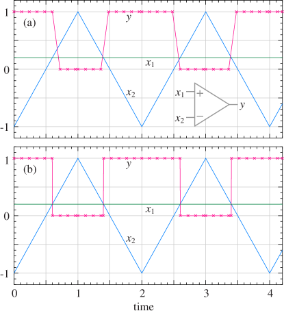
Figure 17: Comparator input and output waveforms: (a) with a constant time step, (b) with additional time points obtained by extrapolation. Crosses show the simulator time points.

For resolving the abrupt transition in $y(t)$ on a shorter time scale but without making the “normal” time step (denoted by $\Delta t_{\mathrm{normal}}$) small, GSEIM uses the following scheme. The comparator template stores the previous time point $t_{-1}$ and the corresponding solutions $x_{1}^{(-1)}$, $x_{2}^{(-1)}$. Knowing these, and the current time point and solutions ($t_{0}$, $x_{1}^{(0)}$, $x_{2}^{(0)}$), it uses linear extrapolation to compute the time $t^{\prime}$ at which $x_{1}-x_{2}$ would cross zero. If $t^{\prime}$ is within $\Delta t_{\mathrm{normal}}$ of $t_{0}$, GSEIM places one time point just before and one time point just after $t^{\prime}$. Fig. 17 (b) shows the waveforms obtained with this method. The transition at $t\,$=$\,2.6$ s is now seen to be resolved properly.

When the linear extrapolation technique is used for the comparator inputs shown in Fig. 18 (a), the zero crossing at $t\approx 1.93\,$s is not treated correctly because linear extrapolation overestimates $t^{\prime}$ in this case, as illustrated in Fig. 19. This problem can be addressed as follows. The comparator stores, in addition to $t_{0}$, $t_{-1}$ (and the corresponding solutions), one more past time point $t_{-2}$ and the corresponding solutions $x_{1}^{(-2)}$, $x_{2}^{(-2)}$. It uses this information to fit a quadratic which passes through $(t_{0},u^{(0)})$, $(t_{-1},u^{(-1)})$, $(t_{-2},u^{(-2)})$, (where $u\equiv x_{1}-x_{2}$), and computes $t^{\prime}$ at which it goes through zero. Fig. 18 (b) shows the waveforms obtained with the quadratic extrapolation scheme. It can be seen that the transition at $t\approx 1.93\,$s is now treated correctly.

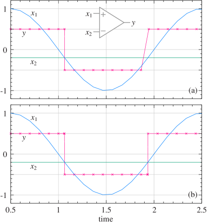
Figure 18: Comparator input and output waveforms: (a) with linear extrapolation, (b) with quadratic extrapolation.

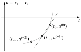
Figure 19: Example of failure of the linear extrapolation technique for treating crossover events.

7 Simulation Examples

We now look at simulation examples which demonstrate the capabilities of GSEIM. We consider two examples, both involving the induction machine model described by Eqs. 6-10. Details regarding setting up the schematic, running the simulation, viewing the plots, will be described in [15] and are not reproduced here. Also, a detailed description of the system being simulated, values of the machine parameters, etc. are not included. The simulation times mentioned in the following are for a desktop computer (Ubuntu-19) with 3.2 GHz clock and 8 GB RAM.

7.1 Free acceleration of induction motor

In this example, we consider free acceleration of an induction motor with load torque $T_{L}\,$=$\,0$. Fig. 20 shows the GSEIM schematic diagram for the system when the induction motor template discussed in Sec. 4 is used. In this case, the conversion of $V_{a}$, $V_{b}$, $V_{c}$ to $V_{d}$, $V_{q}$ is required, and it is performed by the abc_to_dq element. Fig. 21 shows the GSEIM schematic diagram for the same problem when the induction machine subcircuit of Sec. 5 is used. In this case, the $abc$-to-$dq$ conversion is incorporated within the subcircuit. Figs. 22 (a) and 22 (b) show the simulation results for speed and torque, respectively. The capability of GSEIM to produce plots of interest without cluttering the schematic diagram with scopes may be noted.

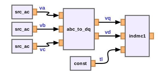
Figure 20: GSEIM schematic diagram for simulation of free acceleration of induction motor using indmc1.xbe

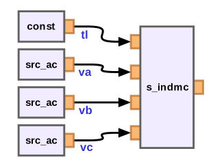
Figure 21: GSEIM schematic diagram for simulation of free acceleration of induction motor using induction machine subcircuit.

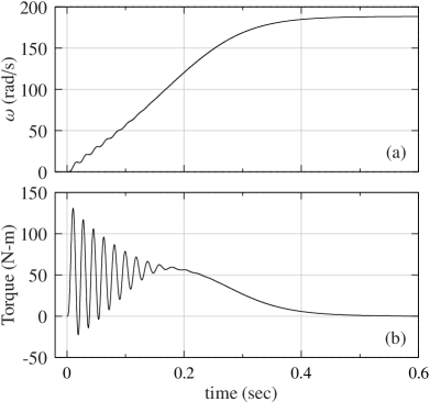
Figure 22: Simulation results for free acceleration of induction motor: (a) speed, (b) torque

7.2 $V/f$ control of induction motor

The GSEIM schematic diagram for $V/f$ control of an induction motor [9] is shown in Fig. 23. The induction machine block shown in the figure corresponds to the subcircuit of Fig. 15; however, we can also use the element template indmc1.xbe (see Sec. 4) directly. The pwl20 element, which allows piecewise linear waveforms, is used to generate the frequency command which is smoothened using the lag_1 element, satisfying

$$\frac{dy}{dt}=\displaystyle\frac{1}{T_{r}}\,(-y+x).$$ (17)

The $V/f$ conversion is provided by pwl10_xy.

Simulation of this system is computationally more demanding than the free acceleration example because (a) its size is larger, (b) accurate resolution of PWM voltages requires smaller time steps. For resolving the PWM waveforms correctly, the linear extrapolation technique described in Sec. 6 has been used. Fig. 24 shows the PWM voltages in steady state. It is seen that the transitions between low and high levels are treated properly. Fig. 25 shows the motor speed versus time.

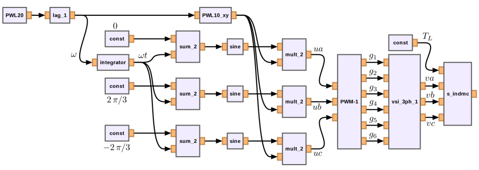
Figure 23: GSEIM schematic diagram for $V/f$ control of an induction motor.

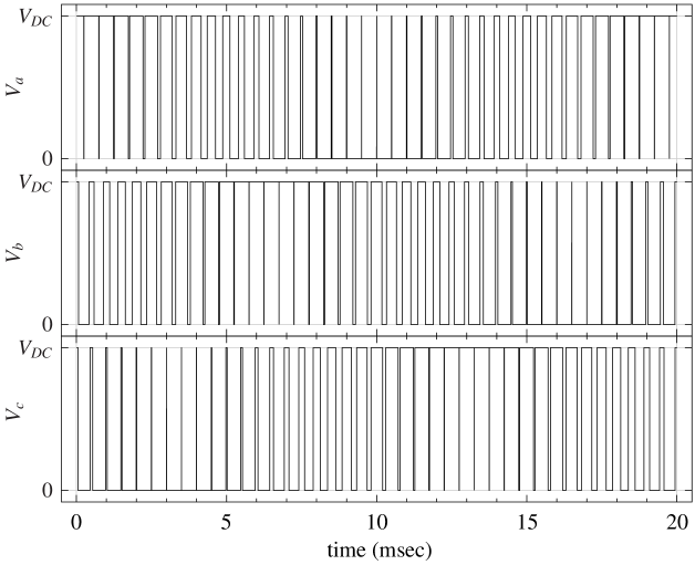
Figure 24: Voltages $V_{a}$, $V_{b}$, $V_{c}$ in steady state for the system of Fig. 23.

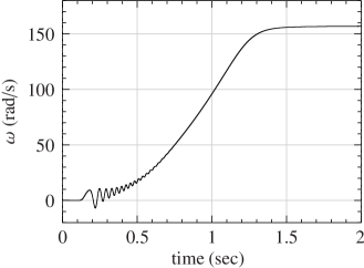
Figure 25: Speed versus time for the system of Fig. 23.

It is interesting to compare the simulation times when two different approaches are used: (a) induction machine as a subcircuit (described in Sec. 5), (b) induction machine as an element template (described in Sec. 4). To enable a fair comparison, the same numerical method (RKF45) was used in both cases, and the algorithmic parameters were kept the same. The simulation times were found to be 2.33 s and 1.55 s, respectively, for (a) and (b). This clearly brings out the advantage of implementing equations at a low level (the template level) rather than as a subcircuit. On the other hand, subcircuit implementation is often easier, and therefore it may be preferred when simulation time is not large enough to be of concern.

8 Conclusions and future work

In summary, we have presented a new general-purpose ODE solver called GSEIM which allows the use of explicit as well as implicit methods. The organisation of the program has been described. A useful feature of GSEIM is that it allows the user to write new templates to incorporate element equations. In addition, it also allows the use of subcircuits (hierarchical blocks). These two facilities are illustrated with the help of examples. The importance of correct handling of abrupt changes is pointed out, and the techniques used by GSEIM to handle abrupt changes are explained. Finally, two representative simulation examples are presented. The computational advantage of incorporating element equations in a basic template rather than a subcircuit is brought out.

The authors plan to make the GSEIM package available under the GNU general public license, after preparing a users’ manual and video tutorials. Further developments in GSEIM are expected to address the following issues.

• Additional features in the schematic capture GUI such as rectangular wires, “bus” facility (i.e., grouping of several connections into a single wire), use of images in the element symbols, provision for adding text to the canvas, etc.

• Allowing electrical type elements, which satisfy some form of Kirchhoff’s current and voltage laws, in addition to the “flow-graph” type elements currently available. This will significantly enhance the applications handled by GSEIM.

References

- [1] Simulink – Simulation and Model-Based Design. [Online]. Available: https://in.mathworks.com/products/simulink.html
- [2] DYMOLA Systems Engineering. [Online]. Available: https://www.3ds.com/products-services/catia/products/dymola/
- [3] Xcos: Dynamic systems modeler. [Online]. Available: https://www.scilab.org/software/xcos
- [4] W.J. McCalla, Fundamentals of Computer-Aided Circuit Simulation. Boston: Kluwer Academic Publishers, 1987.
- [5] L.F. Shampine, Numerical Solution of Ordinary Differential Equations. New York: Chapman and Hall, 1994.
- [6] C.F. Gerald and P.O. Whitley, Applied Numerical Analysis. Delhi: Pearson Education India, 1999.
- [7] S.C. Chapra and R.P. Canale, Numerical Methods for Engineers. New Delhi: Tata McGraw-Hill, 2000.
- [8] R.L. Burden and J.D. Faires, Numerical Analysis. Singapore: Thomson, 2001.
- [9] M.B. Patil, V. Ramanarayanan, and V.T. Ranganathan, Simulation of power electronic circuits. New Delhi: Narosa, 2009.
- [10] R.E. Bank, W.M. Coughran, W. Fichtner, E.H. Grosse, D.J. Rose, and R.K. Smith, “Transient simulation of silicon devices and circuits,” IEEE Trans. Computer-Aided Design of Integrated Circuits and Systems, vol. 4, no. 4, pp. 436–451, 1985.
- [11] GNU Radio Manual and C++ API Reference. [Online]. Available: http://www.gnuradio.org
- [12] OpenModelica. [Online]. Available: https://openmodelica.org/
- [13] Verilog-AMS Language Reference Manual. [Online]. Available: https://www.accellera.org/downloads/standards/v-ams
- [14] P. Nenzi, “Ngspice circuit simulator release 26, 2014.”
- [15] M.B. Patil, “GSEIM users manual,” (under preparation).