Learning How to Ask: Querying LMs with Mixtures of Soft Prompts

Abstract

Natural-language prompts have recently been used to coax pretrained language models into performing other AI tasks, using a fill-in-the-blank paradigm (Petroni et al., 2019) or a few-shot extrapolation paradigm Brown et al. (2020). For example, language models retain factual knowledge from their training corpora that can be extracted by asking them to “fill in the blank” in a sentential prompt. However, where does this prompt come from? We explore the idea of learning prompts by gradient descent—either fine-tuning prompts taken from previous work, or starting from random initialization. Our prompts consist of “soft words,” i.e., continuous vectors that are not necessarily word type embeddings from the language model. Furthermore, for each task, we optimize a mixture of prompts, learning which prompts are most effective and how to ensemble them. Across multiple English LMs and tasks, our approach hugely outperforms previous methods, showing that the implicit factual knowledge in language models was previously underestimated. Moreover, this knowledge is cheap to elicit: random initialization is nearly as good as informed initialization.

1 Introduction

Pretrained language models, such as ELMo (Peters et al., 2018), BERT (Devlin et al., 2019), and BART (Lewis et al., 2020a), have proved to provide useful representations for other NLP tasks. Recently, Petroni et al. (2019) and Jiang et al. (2020) demonstrated that language models (LMs) also contain factual and commonsense knowledge that can be elicited with a prompt. For example, to query the date-of-birth of Mozart, we can use the prompt “MozartwhiteMozart was born in       ,” where we have filled the first blank with “Mozart,” and ask a cloze language model to fill in the second blank. The prompts used by Petroni et al. (2019) are manually created, while Jiang et al. (2020) use mining and paraphrasing based methods to automatically augment the prompt sets.

Finding out what young children know is difficult because they can be very sensitive to the form of the question Donaldson (1978). Opinion polling is also sensitive to question design (Broughton, 1995). We observe that when we are querying an LM rather than a human, we have the opportunity to tune prompts using gradient descent—the workhorse of modern NLP—so that they better elicit the desired type of knowledge.

A neural LM sees the prompt as a sequence of continuous word vectors (Baroni et al., 2014). We tune in this continuous space, relaxing the constraint that the vectors be the embeddings of actual English words. Allowing “soft prompts” consisting of “soft words” is not only convenient for optimization, but is also more expressive. Soft prompts can emphasize particular words (by lengthening their vectors) or particular dimensions of those words. They can also adjust words that are misleading, ambiguous, or overly specific. Consider the following prompt for the relation date-of-death:

       $\!{}_{\mathrm{x}}$ performed until his death in        $\!{}_{\mathrm{y}}$.

This prompt may work for the male singer Cab Calloway, but if we want it to also work for the female painter Mary Cassatt, it might help to soften “performed” and “his” so that they do not insist on the wrong occupation and gender, and perhaps to soften “until” into a weaker connective (as Cassatt was in fact too blind to paint in her final years).

Another way to bridge between these cases is to have one prompt using “performed” and another using “painted.” In general, there may be many varied lexical patterns that signal a particular relation, and having more patterns will get better coverage Hearst (1992); Riloff and Jones (1999). We therefore propose to learn a mixture of soft prompts.

We test the idea on several cloze language models, training prompts to complete factual and common sense relations from 3 datasets. Comparing on held-out examples, our method dramatically outperforms previous work, even when initialized randomly. So when regarded as approximate knowledge bases, language models know more than we realized. We just had to find the right ways to ask.

2 Related Work

Factual knowledge is traditionally extracted from large corpora using a pipeline of NLP tools (Surdeanu and Ji, 2014), including entity extraction (Lample et al., 2016), entity linking (Rao et al., 2013) and relation extraction (Sorokin and Gurevych, 2017).

However, recent work has shown that simply training a system to complete sentences—language modeling—causes it to implicitly acquire non-linguistic abilities from its training corpora (Rogers et al., 2020), including factual knowledge (Petroni et al., 2019; Jiang et al., 2020), common sense (Bisk et al., 2019), reasoning (Talmor et al., 2020; Brown et al., 2020), summarization (Radford et al., 2019), and even arithmetic (Bouraoui et al., 2020).

Most of the previous work manually creates prompts to extract answers from the trained language model. We use LAMA Petroni et al. (2019) as a baseline. Building on LAMA, the LM Prompt And Query Archive (LPAQA) method Jiang et al. (2020) searches for new prompts by either mining a corpus or paraphrasing existing prompts. AutoPrompt Shin et al. (2020) searches for improved prompts using a gradient signal, although its prompts are limited to sequences of actual (“hard”) English words, unlike our method. We compare our novel soft prompts against all of these systems.

After we submitted the present paper in November 2020, two still unpublished manuscripts appeared on arXiv that also investigated soft prompts. Li and Liang (2021) considered the setting of generating text from a pretrained language model (GPT-2 or BART) conditioned on a textual prompt. To improve the results, they prepended a few task-specific “soft tokens” to the prompt and tuned the embeddings of only these tokens (at all embedding layers). Liu et al. (2021) adopted a strategy similar to ours by tuning fill-in-the-blank prompts in a continuous space, testing on GPT-2 and BERT models, although they did not use the enhancements we proposed in §§ 3.2–3.4 below. Like our work, both these papers achieved strong gains.

In other work, Bouraoui et al. (2020) mine prompts from a corpus, then fine-tune the whole language model so that it more accurately completes the prompts. Schick and Schütze (2020a, b) are similar but fine-tune the language model differently for each prompt. Our method complements these by tuning the prompts themselves.

“Probing” systems that ask what language models know about particular sentences (e.g., Eichler et al., 2019) usually use feedforward networks rather than further natural-language prompts. Yet Shin et al. (2020) show how to use natural-language prompts to ask about particular sentences. Our method could potentially be applied to those prompts, or to “few-shot learning” prompts that include input-output examples Brown et al. (2020).

3 Method

Our experiments will specifically aim at extracting relational knowledge from language models. We are given a fixed pretrained LM, a specific binary relation $r$ such as date-of-death, and a training dataset $\mathcal{E}_{r}$ consisting of known $(x,y)$ pairs in $r$, such as (Mary Cassatt, 1926). We will then train a system to predict $y$ from $x$, and evaluate it on held-out $(x,y)$ pairs of the same relation.

A prompt $\mathbf{t}$ is a sentence or phrase that includes two blanks, as illustrated in § 1. To pose the query, we fill the        $\!{}_{\mathrm{x}}$ blank with $x$:

Mary CassattwhiteMary Cassatt performed until his death in        $\!{}_{\mathrm{y}}$.

We can ask the LM for its probability distribution $p_{\mathrm{LM}}(y\mid\mathbf{t},x)$ over single words that can now fill        $\!{}_{\mathrm{y}}$. The correct answer would be 1926.

3.1 Soft Prompts

Suppose the LM identifies the word types with vectors in $\mathbb{R}^{d}$. We also allow $\mathbf{t}$ to be a soft prompt, in which the tokens can be arbitrary vectors in $\mathbb{R}^{d}$:

       $\!{}_{\mathrm{x}}$ $\;v_{1}$ $\;v_{2}$ $\;v_{3}$ $\;v_{4}$ $\;v_{5}$         $\!{}_{\mathrm{y}}$ $\;v_{6}$

We can initialize these vectors to match those of a given hard prompt. (Each token of a hard prompt may be a word, subword, or punctuation mark, according to the tokenization procedure used by the LM.) However, we can then tune the vectors continuously. We do not change the number of vectors or their positions. For the prompt shown above, we have a $6d$-dimensional search space.

3.2 Deeply Perturbed Prompts

For each token $i$ of a prompt, the vector $v_{i}$ enters into the LM’s computations that complete the prompt. For example, a Transformer architecture computes successively deeper contextual embeddings of the token, $v_{i}^{(\ell)}:0\leq\ell\leq L$. Here $v_{i}^{(0)}=v_{i}$ and the embedding $v_{i}^{(\ell)}$ at layer $\ell>0$ is computed from all tokens’ embeddings $v_{j}^{(\ell-1)}$ at the previous layer, using the LM’s parameters.

We can tune the prompt by additively perturbing each $v_{i}^{(\ell)}$ by a small vector $\Delta_{i}^{(\ell)}$ before it is used in further computations. The $\Delta$ vectors for a given hard prompt are initialized to 0 and then tuned.

Perturbing only layer 0 is equivalent to tuning $v_{i}$ directly as in § 3.1. However, if we are more aggressive and perturb all layers, we now have $6d\cdot(L+1)$ parameters to tune a 6-token prompt. The perturbations ($\Delta$ vectors) can be kept small through early stopping or some other form of regularization. Our intuition is that small perturbations will yield more “familiar” activation patterns that are similar to those that the LM was originally trained on. (Li and Liang (2021) tried a rather different approach to preventing overfitting when tuning all layers.)

3.3 Mixture Modeling

Given a set $\mathcal{T}_{r}$ of soft prompts for relation $r$, we can define the ensemble predictive distribution

$$p(y\mid x,r)=\sum_{\mathbf{t}\in\mathcal{T}_{r}}p(\mathbf{t}\mid r)\cdot p_{\mathrm{LM}}(y\mid\mathbf{t},x)$$ (1)

where the learned mixture weights $p(\mathbf{t}\mid r)$ form a distribution over the soft prompts $\mathbf{t}\in\mathcal{T}_{r}$. Ensembling techniques other than mixture-of-experts could also be used, including product-of-experts Jiang et al. (2020).

3.4 Data-Dependent Mixture Modeling

As an extension, we can replace the mixture weights $p(\mathbf{t}\mid r)$ with $p(\mathbf{t}\mid r,x)$, to allow the model to select prompts that are appropriate for the given $x$. For example, a plural noun $x$ might prefer prompts $\mathbf{t}$ that use a plural verb.

While we could directly build a neural softmax model for $p(\mathbf{t}\mid r,x)$, it seems useful to capture the intuition that $\mathbf{t}$ may work better if $x$ is plausible in its        $\!{}_{\mathrm{x}}$. Thus, we instead use Bayes’ Theorem to write $p(\mathbf{t}\mid r,x)$ as proportional to $p(\mathbf{t}\mid r)\cdot p(x\mid\mathbf{t},r)^{1/T}$, where we have included $T$ to modulate the strength of the above intuition. Here $p(\mathbf{t}\mid r)$ is still a learned distribution over prompts, and we use the fixed language model to estimate the second factor as $\sum_{y}p_{\mathrm{LM}}(x,y\mid\mathbf{t})$ (dropping the dependence on $r$ just as we did for the second factor of (1)). $\log T$ is tuned along with all other parameters.

3.5 Training Objective

Given an initial set of prompts $\mathcal{T}_{r}$, we jointly optimize the soft prompts $\mathbf{t}\in\mathcal{T}$ and their mixture weights $p(\mathbf{t}\mid r)$ (and $\log T$ in § 3.4) to minimize the log-loss of the predictive distribution (1):

$$\sum_{(x,y)\in\mathcal{E}_{r}}-\log\sum_{\mathbf{t}\in\mathcal{T}_{r}}p(y\mid\mathbf{t},x)$$ (2)

This is a continuous and differentiable objective whose gradient can be computed by back-propagation. It can be locally minimized by gradient descent (using a softmax parameterization of the mixture weights). Equivalently, it can be locally minimized by the EM algorithm: the E step finds a posterior distribution over latent prompts for each $(x,y)$ example, and the M step performs gradient descent to optimize the prompts in that mixture.

4 Experiments

4.1 Relational Datasets

The relations we learn to predict are T-REx original (Elsahar et al., 2018), T-REx extended (Shin et al., 2020), Google-RE (Orr, 2013), and ConceptNet (Speer et al., 2017)—or rather, the subsets that were used by the LAMA and AutoPrompt papers. See Appendix A for some statistics.

4.2 Language Models

Following Petroni et al. (2019), we interrogate BERT (Devlin et al., 2019) and RoBERTa (Liu et al., 2019). These are masked (cloze) language models. For variety, we also interrogate BART (Lewis et al., 2020a), which conditions on the prompt with empty        $\!{}_{\mathrm{y}}$ and generates a copy where        $\!{}_{\mathrm{y}}$ has been filled in (by a single token). We constrain BART’s decoding to ensure that its answer does take this form. Unlike BERT and RoBERTa, BART could be used to fill        $\!{}_{\mathrm{y}}$ with an arbitrarily long phrase, but we do not allow this because $y$ in our datasets is always a single token.

4.3 Dataset Splits

For the two T-REx datasets, we inherit the training-validation-test split from Shin et al. (2020). For the other datasets, we split randomly in the ratio 80-10-10. Since all pairs $(x,y)$ are distinct, there are no common triples among these three sets. Common $x$ values are also rare because each dataset has at least 174 distinct $x$ values. However, the number of distinct $y$ values can be as small as 6. Thus, in another set of experiments (Appendix E), we used a more challenging split that ensures that there are no common $y$ values among these three sets. This tests whether our model generalizes to unseen values.

4.4 Prompts

For the T-REx and Google-RE datasets, we have four sources of initial prompts:

• (sin.) LAMA provides a single manually created hard prompt for each relation type $r$.

• (par.) LPAQA (Jiang et al., 2020) provides a set of 13–30 hard prompts for each $r$, which are paraphrases of the LAMA prompt.

• (min.) LPAQA also provides a set of 6–29 hard prompts for each $r$, based on text mining.

• (ran.) For each (min.) prompt, we replace each word with a random vector, drawn from a Gaussian distribution fit to all of the LM’s word embeddings. The number of words and the position of the blanks are preserved.

For the ConceptNet dataset, LAMA uses the gold Open Mind Common Sense (OMCS) dataset (Singh et al., 2002). In this dataset, each example $(x_{i},y_{i})$ is equipped with its own prompt $\mathbf{t}_{i}$. (Each example is really a sentence with two substrings marked as $x$ and $y$, which are removed to obtain $\mathbf{t}_{i}$.) These prompts are often overly specific: often $y_{i}$ can be predicted from $(\mathbf{t}_{i},x_{i})$, or just from $\mathbf{t}_{i}$ alone, but $y_{j}$ cannot be predicted from $(\mathbf{t}_{i},x_{j})$. Thus, for each relation $r$, we use only the prompts that appear more than 10 times, resulting in 1–38 prompts.

Statistics about the prompts are in Appendix B.

We used only a single copy of each prompt, but a generalization would be to allow multiple slightly perturbed copies of each prompt, which could diverge and specialize during training Rose (1998).

4.5 Training

We optimize equation 2 with the method introduced in § 3.5. We use the Adam optimizer (Kingma and Ba, 2015) with its default configuration. For gradient training, we set the batch size as 64, early-stop patience as 4, and test with the model that performs best on the dev set among 16 training epochs.

Training is fast. Even for our largest model (BERT-large-cased) and largest dataset (T-REx extended), tuning a single prompt completes within a few minutes. With a mixture of prompts, training scales roughly linearly with the number of prompts. It is still presumably much cheaper in time and memory than fine-tuning the entire BERT model, which must back-propagate a much larger set of gradients.

4.6 Metrics and Baselines

Our method outputs the most probable $y$ given $(r,x)$. Here and in the supplementary material, we report its average performance on all test examples, with precision-at-1 (P@1), precision-at-10 (P@10) and mean reciprocal rank (MRR) as metrics. We measure the improvement from tuning LAMA, LPAQA, and random prompts. We also compare with AutoPrompt. Baseline numbers come from prior papers or our reimplementations.

4.7 Results

Model	T-REx orig.	T-REx ext.
lama (BEb)	31.1	26.4
lpaqa(BEb)	34.1	31.2
AutoPrompt	43.3	45.6
Soft (sin., BEb)	47.7 (+16.6?)	49.6 (+23.2?)
Soft (min., BEb)	50.7?(+16.6?)	50.5?(+19.3?)
Soft (par., BEb)	48.4 (+12.8?)	49.7 (+18.5?)
Soft (ran., BEb)	48.1 (+47.4)	50.6 (+49.8)
lama (BEl)	28.9†	24.0†
lpaqa(BEl)	39.4†	37.8†
Soft (sin., BEl)	51.1 (+22.2)	51.4 (+27.4)
Soft (min., BEl)	51.6 (+12.2)	52.5 (+14.7)
Soft (par., BEl)	51.1 (+11.7)	51.7 (+13.9)
Soft (ran., BEl)	51.9 (+47.1)	51.9 (+50.5)
AutoPrompt	40.0	-
Soft (min., Rob)	40.6?(+39.4)	-

Table 1: Results on T-REx datasets with P@1 as the metric. The “Soft” lines (our method) parenthetically show the improvement over the initial parameters (boldfaced if significant). In each subcolumn of comparable results, we boldface the best result along with all that are not significantly worse (sign test, $p<0.02$). (We marked a boldface number with "?" if we lacked access to per-example output for one of the systems; differences from such systems were simply assumed to be significant.) ^† marks baseline results obtained from our reimplementations. In the Model column, BEb is BERT-base, BEl is BERT-large, Rob is RoBERTa-base.

Table 1 shows results on T-REx datasets obtained by querying three BERT-style models, with P@1 as the metric. Additional metrics and language models are shown in Tables 2 and 3 as well as Tables 5 and 6 in the supplementary material.

We consistently get large improvements by tuning the initial prompts. Remarkably, our method beats all prior methods even when throwing away the words of their informed prompts in favor of random initial vectors. It simply finds a prompt that works well on the $(x,y)$ training examples.

Model	P@1	P@10	MRR
lama	9.7†	27.0†	15.6†
lpaqa	10.6†	23.7†	15.3†
Soft (sin.)	11.2 (+1.5)	33.5 (+  6.5)	18.9 (+3.3)
Soft (min.)	12.9 (+2.3)	34.7 (+11.0)	20.3 (+5.0)
Soft (par.)	11.5 (+0.9)	31.4 (+  7.7)	18.3 (+3.0)

Table 2: Results on Google-RE dataset obtained by querying the BERT-large-cased model.

Model	P@1	P@10	MRR
lama (BEb)	0.1†	2.6†	1.5†
lama (BEl)	0.1†	5.0†	1.9†
Soft (min.,BEb)	11.3(+11.2)	36.4(+33.8)	19.3(+17.8)
Soft (ran.,BEb)	11.8(+11.8)	34.8(+31.9)	19.8(+19.6)
Soft (min.,BEl)	12.8(+12.7)	37.0(+32.0)	20.9(+19.0)
Soft (ran.,BEl)	14.5(+14.5)	38.6(+34.2)	22.1(+21.9)

Table 3: Results on ConceptNet (winner: random init).

Model	P@1	P@10	MRR
baseline	39.4	67.4	49.1
adjust mixture weights	40.0	69.1	53.3
adjust token vectors	50.7	80.7	61.1
adjust both	51.0	81.4	61.6

Table 4: Ablation experiments, conducted with the BERT-large model on the T-REx original dataset.

We conduct an ablation study where we adjust only the mixture weights (which are initially uniform) or only the word vectors in the prompts $\mathbf{t}$. As Table 4 shows, each helps, but the major benefit comes from tuning the word vectors to get soft prompts. Appendix C visualizes a set of soft prompts, and Appendix D analyzes the mixture weights. We also experiment on a challenging setting where the $y$ labels are distinct for training and test (Appendix E in the supplementary materials), and find that soft prompts still yield some benefits.

The above results are for our basic method that tunes only the words of the prompt (i.e., layer 0). When we tune all layers—the “deeply perturbed prompts” of § 3.2—we typically obtain small additional gains, across various models and initializations, although tuning all layers does substantially hurt RoBERTa. These results are shown in Tables 5 and 6 in the supplementary material.

The tables show that the winning system—for each combination of language model, T-REx dataset, and evaluation metric—always uses a mixture of soft prompts initialized to mined prompts. It always tunes all layers, except with RoBERTa.

Finally, we also tried using data-dependent mixture weights as in § 3.4. This had little effect, because training learned to discard the $x$ information by setting the temperature parameter $T$ high.

5 Conclusion

Well-crafted natural language prompts are a powerful way to extract information from pretrained language models. In the case of cloze prompts used to query BERT and BART models for single-word answers, we have demonstrated startlingly large and consistent improvements from rapidly learning prompts that work—even though the resulting “soft prompts” are no longer natural language.

Our code and data are available at https://github.com/hiaoxui/soft-prompts.

How about few-shot prediction with pretrained generative LMs? Here, Lewis et al. (2020b) show how to assemble a natural language prompt for input $x$ from relevant input-output pairs $(x_{i},y_{i})$ selected by a trained retrieval model. Allowing fine-tuned soft string pairs is an intriguing future possibility for improving such methods without needing to fine-tune the entire language model.

Appendix A Statistics of Relational Databases

The statistics of the various relational databases are shown in Table 8.

Appendix B Statistics of the Initial Prompts

Table 7 shows some statistics of the prompts we use to initialize the SoftPrompt model.

Appendix C Visualization of Soft Prompts

Figure 1 shows what a mixture of soft prompts looks like when we tune only layer 0. The soft prompts are not too interpretable. The words closest to the tuned tokens (shown in blue) seem to be largely on the music topic. However, the soft templates do not seem to form meaningful phrases, nor is it obvious why they would prime for $y$ to be an instrument when $x$ is a musician.

Appendix D Entropy of the Mixture Model

For any given relation $r$, the entropy of the mixture weights is

$$H =\sum_{\mathbf{t}\in\mathcal{T}_{r}}p(\mathbf{t}\mid r)\cdot\log_{2}p(\mathbf{t}\mid r)$$ (3)

We then take $2^{H}\in[1,|\mathcal{T}_{r}|]$ as a measure of the effective number of prompts that were retained. Table 10 shows some statistics of the effective number of prompts. In some cases, tuning the mixture weights essentially selected a single prompt, but on average, it settled on a mixture of several variant prompts (as illustrated by Figure 1).

Appendix E Challenging dataset with distinct $y$’s

As described in § 4.3, we conducted an additional experiment to determine whether the prompts could generalize to novel $y$ values. We conduct another experiment and ensure that there are no common $y$ values among the train / dev / test sets. We use T-REx as the base relational database and split the datasets to make the ratio close to 80-10-10. The experiment results are shown in Table 9. We can observe that our method again improves the results, just as in Tables 5 and 6, which shows the generalizability of our method.

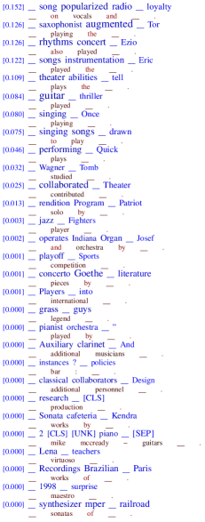
Figure 1: Visualization of the LPAQA mining prompts for relation P1303 Instrument (i.e., $x$ plays instrument $y$) from T-REx extended. We show the effect of tuning the layer-0 token embeddings (but not higher layers) on BERT-large-cased. The prompts are sorted in decreasing order by mixture weight. Each prompt’s weight is shown at left; note that after the first 12 prompts, the remaining ones have negligible contribution. We show each soft prompt in blue, followed by the original (mined) prompt in red. To visualize the tuned vector $\mathbf{v}$, we display the blue word $w$ that maximizes $p(w\mid\mathbf{v})$. The brightness of the blue word $w$ and the original red word $w_{0}$ are respectively proportional to $p(w\mid\mathbf{v})$ and $p(w_{0}\mid\mathbf{v})$. The red word has size 1, and the blue word has size $||\mathbf{v}||/||\mathbf{v}_{0}||$, where $\mathbf{v}_{0}$ is the original untuned vector (the embedding of $w_{0}$). In this example, the blue probabilities $p(w\mid\mathbf{v})$ range from 6.5e-5 to 9.7e-5 (mean 8.6e-5 $\pm$ 8.1e-6), the red probabilities $p(w_{0}\mid\mathbf{v})$ range from 7.7e-5 to 1.1e-4 (mean 9.5e-5 $\pm$ 7.8e-6), and the relative magnitudes $||\mathbf{v}||/||\mathbf{v}_{0}||$ vary from 1.00 to 1.49 (mean 1.12 $\pm$ 0.13).

LM	Method	Precision@1	Precision@10	MRR
		init    $\rightarrow$    soft    $\rightarrow$    deep	init    $\rightarrow$    soft    $\rightarrow$    deep	init    $\rightarrow$    soft    $\rightarrow$    deep
BEb	lama	31.1	59.5	40.3
	lpaqa	34.1	62.0	43.6
	Soft (sin.)	31.1 $\xrightarrow{\mathbf{+14.6^{?}}}$ 45.7 $\xrightarrow{\mathbf{+\ \ 2.0}}$ 47.7	59.5 $\xrightarrow{\mathbf{+16.3^{?}}}$ 75.8 $\xrightarrow{\mathbf{+\ \ 3.2}}$ 79.0	40.3 $\xrightarrow{\mathbf{+15.9^{?}}}$ 56.2 $\xrightarrow{\mathbf{+\ \ 2.2}}$ 58.4
	Soft (min.)	34.1 $\xrightarrow{\mathbf{+14.7^{?}}}$ 48.8 $\xrightarrow{\mathbf{+\ \ 1.9}}$ 50.7?	62.0 $\xrightarrow{\mathbf{+15.6^{?}}}$ 79.6 $\xrightarrow{\mathbf{+\ \ 1.1}}$ 80.7?	43.6 $\xrightarrow{\mathbf{+15.8^{?}}}$ 59.4 $\xrightarrow{\mathbf{+\ \ 1.7}}$ 61.1?
	Soft (par.)	34.1 $\xrightarrow{\mathbf{+12.8^{?}}}$ 46.9 $\xrightarrow{\mathbf{+\ \ 1.5}}$ 48.4	62.0 $\xrightarrow{\mathbf{+16.8^{?}}}$ 78.8 $\xrightarrow{\mathbf{+\ \ 0.8}}$ 79.6	43.6 $\xrightarrow{\mathbf{+14.2^{?}}}$ 57.8 $\xrightarrow{\mathbf{+\ \ 1.3}}$ 59.1
	Soft (ran.)	0.7 $\xrightarrow{\mathbf{+46.6\ \ }}$ 47.3 $\xrightarrow{\mathbf{+\ \ 0.8}}$ 48.1	4.6 $\xrightarrow{\mathbf{+74.0\ \ }}$ 79.1 $\xrightarrow{+\ \ 0.0}$ 79.1	2.3 $\xrightarrow{\mathbf{+56.1\ \ }}$ 58.4 $\xrightarrow{\mathbf{+\ \ 0.5}}$ 58.9
BEl	lama	28.9†	57.7†	38.7†
	lpaqa	39.4†	67.4†	49.1†
	Soft (sin.)	28.9 $\xrightarrow{\mathbf{+16.9}}$ 45.8 $\xrightarrow{\mathbf{+\ \ 5.3}}$ 51.1	57.7 $\xrightarrow{\mathbf{+19.0}}$ 76.7 $\xrightarrow{\mathbf{+\ \ 4.4}}$ 81.1	38.7 $\xrightarrow{\mathbf{+17.8}}$ 56.5 $\xrightarrow{\mathbf{+\ \ 5.0}}$ 61.5
	Soft (min.)	39.4 $\xrightarrow{\mathbf{+11.6}}$ 51.0 $\xrightarrow{\mathbf{+\ \ 0.6}}$ 51.6	67.4 $\xrightarrow{\mathbf{+14.0}}$ 81.4 $\xrightarrow{\mathbf{+\ \ 0.5}}$ 81.9	49.1 $\xrightarrow{\mathbf{+12.5}}$ 61.6 $\xrightarrow{\mathbf{+\ \ 0.5}}$ 62.1
	Soft (par.)	39.4 $\xrightarrow{\mathbf{+\ \ 9.2}}$ 48.6 $\xrightarrow{\mathbf{+\ \ 2.5}}$ 51.1	67.4 $\xrightarrow{\mathbf{+12.6}}$ 80.0 $\xrightarrow{\mathbf{+\ \ 1.7}}$ 81.7	49.1 $\xrightarrow{\mathbf{+10.5}}$ 59.6 $\xrightarrow{\mathbf{+\ \ 2.1}}$ 61.7
	Soft (ran.)	2.3 $\xrightarrow{\mathbf{+47.1}}$ 49.4 $\xrightarrow{\mathbf{+\ \ 1.9}}$ 51.3	8.0 $\xrightarrow{\mathbf{+73.0}}$ 81.0 $\xrightarrow{\mathbf{+\ \ 0.7}}$ 81.7	4.5 $\xrightarrow{\mathbf{+55.9}}$ 60.4 $\xrightarrow{\mathbf{+\ \ 1.5}}$ 61.9
Rob	lpaqa	1.2†	9.1†	4.2†
	AutoPrompt	40.0	68.3	49.9
	Soft (min.)	1.2 $\xrightarrow{\mathbf{+39.4}}$ 40.6 $\xrightarrow{\mathbf{-\ \ 7.3}}$ 33.2	9.1 $\xrightarrow{\mathbf{+66.3}}$ 75.4 $\xrightarrow{\mathbf{-22.3}}$ 53.0	4.2 $\xrightarrow{\mathbf{+48.8}}$ 53.0 $\xrightarrow{\mathbf{-12.1}}$ 40.8
BAb	lpaqa	0.8†	5.7†	2.9†
	Soft (min.)	0.8 $\xrightarrow{\mathbf{+39.1}}$ 39.9	5.7 $\xrightarrow{\mathbf{+69.7}}$ 75.4	2.9 $\xrightarrow{\mathbf{+49.2}}$ 52.1
BAl	lpaqa	3.5†	5.6†	4.8†
	Soft (min.)	3.5 $\xrightarrow{\mathbf{+22.3}}$ 25.8	5.6 $\xrightarrow{\mathbf{+62.4}}$ 68.0	4.8 $\xrightarrow{\mathbf{+36.2}}$ 41.0

Table 5: Experimental results on T-REx original datasets. In the LM column, BEb is BERT-base-cased, BEl is BERT-large-cased, BAb is BART-base-cased, BAl is BART-large-cased, Rob is RoBERTa-base, and Rol is RoBERTa-large. In the results block, “init” uses the initial untuned prompts; “soft” starts at “init” and tunes the prompts (layer 0) and mixture weights; and “deep” starts at “init” and tunes all the layers. Numbers above the arrows are the relative change in the performance. Within each block, we boldface the best system and all those that are not significantly worse (paired permutation test, $p<0.02$). We also boldface the relative changes that are significantly different from 0. Other symbols are as in Table 1.

LM	Method	Precision@1	Precision@10	MRR
		init    $\rightarrow$    soft    $\rightarrow$    deep	init    $\rightarrow$    soft    $\rightarrow$    deep	init    $\rightarrow$    soft    $\rightarrow$    deep
BEb	lama	26.4	54.3	35.8
	lpaqa	31.2	57.3	39.9
	Soft (sin.)	26.4 $\xrightarrow{\mathbf{+22.2^{?}}}$ 48.6 $\xrightarrow{\mathbf{+\ \ 1.0}}$ 49.6	54.3 $\xrightarrow{\mathbf{+23.3^{?}}}$ 77.6 $\xrightarrow{\mathbf{+\ \ 0.3}}$ 77.9	35.8 $\xrightarrow{\mathbf{+22.9^{?}}}$ 58.7 $\xrightarrow{\mathbf{+\ \ 0.6}}$ 59.3
	Soft (min.)	31.2 $\xrightarrow{\mathbf{+19.0^{?}}}$ 50.2 $\xrightarrow{\mathbf{+\ \ 0.3}}$ 50.5?	57.3 $\xrightarrow{\mathbf{+21.9^{?}}}$ 79.2 $\xrightarrow{\mathbf{+\ \ 0.5}}$ 79.7?	39.9 $\xrightarrow{\mathbf{+20.2^{?}}}$ 60.1 $\xrightarrow{\mathbf{+\ \ 0.4}}$ 60.5?
	Soft (par.)	31.2 $\xrightarrow{\mathbf{+18.5^{?}}}$ 49.7 $\xrightarrow{+\ \ 0.0}$ 49.7	57.3 $\xrightarrow{\mathbf{+21.3^{?}}}$ 78.6 $\xrightarrow{\mathbf{+\ \ 0.6}}$ 79.2	39.9 $\xrightarrow{\mathbf{+19.6^{?}}}$ 59.5 $\xrightarrow{\mathbf{+\ \ 0.3}}$ 59.8
	Soft (ran.)	0.8 $\xrightarrow{\mathbf{+46.3\ \ \ }}$ 47.1 $\xrightarrow{\mathbf{+\ \ 3.5}}$ 50.6	4.0 $\xrightarrow{\mathbf{+70.4\ \ \ }}$ 74.4 $\xrightarrow{\mathbf{+\ \ 4.9}}$ 79.3	2.2 $\xrightarrow{\mathbf{+54.3\ \ \ }}$ 56.5 $\xrightarrow{\mathbf{+\ \ 3.9}}$ 60.4
BEl	lama	24.0†	53.7†	34.1†
	lpaqa	37.8†	64.4†	44.0†
	Soft (sin.)	24.0 $\xrightarrow{\mathbf{+26.2}}$ 50.2 $\xrightarrow{\mathbf{+\ \ 1.2}}$ 51.4	53.7 $\xrightarrow{\mathbf{+24.9}}$ 78.6 $\xrightarrow{\mathbf{+\ \ 0.9}}$ 79.5	34.1 $\xrightarrow{\mathbf{+25.9}}$ 60.0 $\xrightarrow{\mathbf{+\ \ 1.2}}$ 61.2
	Soft (min.)	37.8 $\xrightarrow{\mathbf{+13.4}}$ 51.2 $\xrightarrow{\mathbf{+\ \ 1.3}}$ 52.5	64.4 $\xrightarrow{\mathbf{+15.1}}$ 79.5 $\xrightarrow{\mathbf{+\ \ 1.6}}$ 81.1	44.0 $\xrightarrow{\mathbf{+17.0}}$ 61.0 $\xrightarrow{\mathbf{+\ \ 1.4}}$ 62.4
	Soft (par.)	37.8 $\xrightarrow{\mathbf{+12.5}}$ 50.3 $\xrightarrow{\mathbf{+\ \ 1.4}}$ 51.7	64.4 $\xrightarrow{\mathbf{+14.3}}$ 78.7 $\xrightarrow{\mathbf{+\ \ 2.1}}$ 80.8	44.0 $\xrightarrow{\mathbf{+16.1}}$ 60.1 $\xrightarrow{\mathbf{+\ \ 1.6}}$ 61.7
	Soft (ran.)	1.4 $\xrightarrow{\mathbf{+46.1}}$ 47.5 $\xrightarrow{\mathbf{+\ \ 4.4}}$ 51.9	5.4 $\xrightarrow{\mathbf{+68.9}}$ 74.3 $\xrightarrow{\mathbf{+\ \ 6.3}}$ 80.6	5.7 $\xrightarrow{\mathbf{+51.2}}$ 56.9 $\xrightarrow{\mathbf{+\ \ 5.0}}$ 61.9

Table 6: Experiment results on T-REx extended datasets.

prompts	T-REx-min.	T-REx-par.	Goog-sin.	Goog-min.	Goog-par.	ConceptNet
#relations	41	41	3	3	3	16
avg. prompts	28.4	26.2	1	32.7	28.0	9.3
min #prompts	6	13	1	29	24	1
max #prompts	29	30	1	40	30	38
avg. #tokens	5.1	4.5	4.7	5.3	4.2	7.1

Table 7: Statistics of prompts. The “Goog” stands for “Google-RE.” We do not list the statistics of randomized prompts, as they should match the statistics of the mined prompts (“min.”) from which they are derived.

database	T-REx original	T-REx extended	Google-RE	ConceptNet
#relations	41	41	3	16
avg. #unique $x$	1580	834	1837	511
avg. #unique $y$	217	151	372	507
min #$(x,y)$	544	310	766	510
max #$(x,y)$	1982	1000	2937	4000
mean #$(x,y)$	1715	885	1843	1861

Table 8: Statistics of the relational databases.

Model	P@1	P@10	MRR
lpaqa (BEb)	18.9	40.4	26.6
Soft (BEb)	23.0 (+4.1)	45.2 (+4.8)	30.5 (+3.9)
lpaqa (BEl)	23.8	47.7	32.2
Soft (BEl)	27.0 (+3.2)	51.7 (+4.0)	35.4 (+3.2)

Table 9: Results with distinct $y$’s. We use the BERT-base-cased and BERT-large-cased LMs and the LPAQA mining based prompts as initial prompts. The experiments are conducted on the T-REx original dataset.

statistic	mean	std	min	max
T-REx original + min.	12.5	4.0	4.6	21.0
T-REx extended + min.	12.5	4.0	4.6	20.3
T-REx original + par.	5.4	4.0	1.1	17.1
T-REx extended + par.	5.4	3.9	1.2	18.4

Table 10: Statistics of effective number of prompts.

References

- Baroni et al. (2014) Marco Baroni, Georgiana Dinu, and Germán Kruszewski. 2014. Don’t count, predict! A systematic comparison of context-counting vs. context-predicting semantic vectors. In Association for Computational Linguistics (ACL), pages 238–247.
- Bisk et al. (2019) Yonatan Bisk, Rowan Zellers, Ronan Le Bras, Jianfeng Gao, and Yejin Choi. 2019. PIQA: Reasoning about physical commonsense in natural language. In Association for the Advancement of Artificial Intelligence (AAAI).
- Bouraoui et al. (2020) Zied Bouraoui, Jose Camacho-Collados, and Steven Schockaert. 2020. Inducing relational knowledge from BERT. In Association for the Advancement of Artificial Intelligence (AAAI), volume 34, pages 7456–7463.
- Broughton (1995) David Broughton. 1995. The assumptions and theory of public opinion polling. In Public Opinion Polling and Politics in Britain, pages 15–33. Springer.
- Brown et al. (2020) Tom B. Brown, Benjamin Mann, Nick Ryder, Melanie Subbiah, Jared Kaplan, Prafulla Dhariwal, Arvind Neelakantan, Pranav Shyam, Girish Sastry, Amanda Askell, Sandhini Agarwal, Ariel Herbert-Voss, Gretchen Krueger, Tom Henighan, Rewon Child, Aditya Ramesh, Daniel M. Ziegler, Jeffrey Wu, Clemens Winter, Christopher Hesse, Mark Chen, Eric Sigler, Mateusz Litwin, Scott Gray, Benjamin Chess, Jack Clark, Christopher Berner, Sam McCandlish, Alec Radford, Ilya Sutskever, and Dario Amodei. 2020. Language models are few-shot learners.
- Devlin et al. (2019) J. Devlin, M. Chang, K. Lee, and K. Toutanova. 2019. BERT: Pre-training of deep bidirectional transformers for language understanding. In North American Association for Computational Linguistics (NAACL).
- Donaldson (1978) M. C. Donaldson. 1978. Children’s Minds. W. W. Norton.
- Eichler et al. (2019) Max Eichler, Gözde Gül Şahin, and Iryna Gurevych. 2019. LINSPECTOR WEB: A multilingual probing suite for word representations. In Proceedings of the 2019 Conference on Empirical Methods in Natural Language Processing and the 9th International Joint Conference on Natural Language Processing (EMNLP-IJCNLP): System Demonstrations, pages 127–132.
- Elsahar et al. (2018) Hady Elsahar, Pavlos Vougiouklis, Arslen Remaci, Christophe Gravier, Jonathon Hare, Elena Simperl, and Frederique Laforest. 2018. T-REx: A large scale alignment of natural language with knowledge base triples. In Language Resources and Evaluation Conference (LREC), page 5.
- Hearst (1992) M. A. Hearst. 1992. Automatic acquisition of hyponyms from large text corpora. In International Conference on Computational Linguistics (COLING).
- Jiang et al. (2020) Zhengbao Jiang, Frank F. Xu, Jun Araki, and Graham Neubig. 2020. How can we know what language models know? Transactions of the Association for Computational Linguistics (TACL).
- Kingma and Ba (2015) D. P. Kingma and J. L. Ba. 2015. Adam: A method for stochastic optimization. In International Conference on Learning Representations (ICLR), pages 1–15.
- Lample et al. (2016) Guillaume Lample, Miguel Ballesteros, Sandeep Subramanian, Kazuya Kawakami, and Chris Dyer. 2016. Neural architectures for named entity recognition. In North American Association for Computational Linguistics and Human Language Technology (NAACL-HLT), pages 260–270.
- Lewis et al. (2020a) Mike Lewis, Yinhan Liu, Naman Goyal, Marjan Ghazvininejad, Abdelrahman Mohamed, Omer Levy, Ves Stoyanov, and Luke Zettlemoyer. 2020a. BART: Denoising sequence-to-sequence pre-training for natural language generation, translation, and comprehension. In Association for Computational Linguistics (ACL).
- Lewis et al. (2020b) Patrick Lewis, Ethan Perez, Aleksandara Piktus, Fabio Petroni, Vladimir Karpukhin, Naman Goyal, Heinrich Küttler, Mike Lewis, Wen tau Yih, Tim Rocktäschel, Sebastian Riedel, and Douwe Kiela. 2020b. Retrieval-augmented generation for knowledge-intensive NLP tasks. arXiv preprint arXiv:2005.11401.
- Li and Liang (2021) Xiang Lisa Li and Percy Liang. 2021. Prefix-tuning: Optimizing continuous prompts for generation. arXiv preprint arXiv:2101.00190.
- Liu et al. (2021) Xiao Liu, Yanan Zheng, Zhengxiao Du, Ming Ding, Yujie Qian, Zhilin Yang, and Jie Tang. 2021. GPT understands, too. arXiv preprint arXiv:2103.10385.
- Liu et al. (2019) Y. Liu, M. Ott, N. Goyal, J. Du, M. Joshi, D. Chen, O. Levy, M. Lewis, L. S. Zettlemoyer, and V. Stoyanov. 2019. RoBERTa: A robustly optimized BERT pretraining approach.
- Orr (2013) Dave Orr. 2013. 50,000 lessons on how to read: A relation extraction corpus. https://github.com/google-research-datasets/relation-extraction-corpus.
- Peters et al. (2018) M. E. Peters, M. Neumann, M. Iyyer, M. Gardner, C. Clark, K. Lee, and L. S. Zettlemoyer. 2018. Deep contextualized word representations. In North American Association for Computational Linguistics (NAACL).
- Petroni et al. (2019) F. Petroni, T. Rocktäschel, P. Lewis, A. Bakhtin, Y. Wu, A. H. Miller, and S. Riedel. 2019. Language models as knowledge bases? In Empirical Methods in Natural Language Processing (EMNLP).
- Radford et al. (2019) Alec Radford, Jeffrey Wu, Rewon Child, David Luan, Dario Amodei, and Ilya Sutskever. 2019. Language models are unsupervised multitask learners.
- Rao et al. (2013) Delip Rao, Paul McNamee, and Mark Dredze. 2013. Entity linking: Finding extracted entities in a knowledge base. In Multi-Source, Multilingual Information Extraction and Summarization, pages 93–115. Springer.
- Riloff and Jones (1999) E. Riloff and R. Jones. 1999. Learning dictionaries for information extraction by multi-level bootstrapping. In Association for the Advancement of Artificial Intelligence (AAAI), pages 474–479.
- Rogers et al. (2020) Anna Rogers, Olga Kovaleva, and Anna Rumshisky. 2020. A primer in BERTology: What we know about how BERT works. Transactions of the Association for Computational Linguistics (TACL).
- Rose (1998) Kenneth Rose. 1998. Deterministic annealing for clustering, compression, classification, regression, and related optimization problems. Proceedings of the IEEE, 80:2210–2239.
- Schick and Schütze (2020a) Timo Schick and Hinrich Schütze. 2020a. Exploiting cloze questions for few-shot text classification and natural language inference. arXiv preprint arXiv:2001.07676. Accepted to EACL 2021.
- Schick and Schütze (2020b) Timo Schick and Hinrich Schütze. 2020b. It’s not just size that matters: Small language models are also few-shot learners. arXiv preprint arXiv:2009.07118.
- Shin et al. (2020) Taylor Shin, Yasaman Razeghi, Robert L. Logan IV, Eric Wallace, and Sameer Singh. 2020. AutoPrompt: Eliciting knowledge from language models with automatically generated prompts. In Empirical Methods in Natural Language Processing (EMNLP).
- Singh et al. (2002) Push Singh, Thomas Lin, Erik T. Mueller, Grace Lim, Travell Perkins, and Wan Li Zhu. 2002. Open Mind Common Sense: Knowledge acquisition from the general public. In On the Move to Meaningful Internet Systems 2002: CoopIS, DOA, and ODBASE, volume 2519, pages 1223–1237. Springer.
- Sorokin and Gurevych (2017) Daniil Sorokin and Iryna Gurevych. 2017. Context-aware representations for knowledge base relation extraction. In Empirical Methods in Natural Language Processing (EMNLP), pages 1784–1789.
- Speer et al. (2017) R. Speer, J. Chin, and C. Havasi. 2017. ConceptNet 5.5: An open multilingual graph of general knowledge. In Association for the Advancement of Artificial Intelligence (AAAI).
- Surdeanu and Ji (2014) Mihai Surdeanu and Heng Ji. 2014. Overview of the English slot filling track at the TAC2014 knowledge base population evaluation. In Proceedings of the TAC-KBP 2014 Workshop.
- Talmor et al. (2020) Alon Talmor, Yanal Elazar, Yoav Goldberg, and Jonathan Berant. 2020. oLMpics – On what language model pre-training captures. Transactions of the Association for Computational Linguistics, 8:743–758.