A Novel Generalised Meta-Heuristic Framework for Dynamic Capacitated Arc Routing Problems

Abstract

The capacitated arc routing problem (CARP) is a challenging combinatorial optimisation problem abstracted from many real-world applications, such as waste collection, road gritting and mail delivery. However, few studies considered dynamic changes during the vehicles’ service, which can cause the original schedule infeasible or obsolete. The few existing studies are limited by the dynamic scenarios considered, and by overly complicated algorithms that are unable to benefit from the wealth of contributions provided by the existing CARP literature. In this paper, we first provide a mathematical formulation of dynamic CARP (DCARP) and design a simulation system that is able to consider dynamic events while a routing solution is already partially executed. We then propose a novel framework which can benefit from existing static CARP optimisation algorithms so that they could be used to handle DCARP instances. The framework is very flexible. In response to a dynamic event, it can use either a simple restart strategy or a sequence transfer strategy that benefits from past optimisation experience. Empirical studies have been conducted on a wide range of DCARP instances to evaluate our proposed framework. The results show that the proposed framework significantly improves over state-of-the-art dynamic optimisation algorithms.

I Introduction

The Capacitated Arc Routing Problem (CARP) is a classical combinatorial optimisation problem with a range of collection and delivery applications in the real world. For example, in a waste collection problem [1], the capacitated vehicles start from a depot to collect the waste distributed in different streets. In a winter road gritting problem, which is a kind of delivery application [2], the fully loaded vehicles deliver the salt to spread into different required roads. Such scenarios are the main focus in this paper.

Constructive heuristic methods, such as Ulusoy’s split [3] and Path-Scanning [4], were proposed to construct feasible executable solutions for CARP based on an optimised sequence of tasks. Tabu search [5], memetic algorithms [6] and others were also proposed to solve the CARP. In addition, efficient algorithms have been proposed to tackle large scale CARPs [7, 8]. Many different variants of CARP have been investigated [9, 10]. For example, multi-depot CARP considers several different depots in the graph [11], and open CARP allows the routes to be open with different starting and ending nodes [12]. Split-delivery CARP allows the edge demand to be served by several vehicles [13]. Periodic CARP considers the cases where the tasks are required to be served with a certain number of times over a given multiperiod horizon [14]. Time CARP considers the time instead of the volume restriction of the vehicles [15].

However, all these studies concentrate on static CARPs, where the problem remains static during the entire time of a solution’s execution. In real applications, dynamic changes usually happen when vehicles are in service, i.e., when a solution is partially executed, thus influencing the vehicles’ follow-on service. For example, a road may be closed due to an accident or new tasks may emerge during the vehicles’ service. When that happens, a new graph, i.e. a new problem instance, is formed, in which vehicles would stop at different locations, labelled as outside vehicles, with various amounts of remaining capacities. As a result, the current schedule may become inferior or even feasible. Dynamic CARP (DCARP) in our paper thus aims at re-scheduling the service plan [16, 17]. For clarity, the following three different concepts are used throughout our paper:

• DCARP: A variant of CARP where the status of a graph is changed due to dynamic events occurring during a CARP solution’s execution.

• DCARP Instance: The updated graph with some outside vehicles after the dynamic events happen.

• DCARP Scenario: A scenario contains a series of DCARP instances with the whole service process, starting from executing an initial solution in the original CARP map until all tasks are served.

It is worth noting that Mei et al. [18] used the term DCARP to denote the uncertain CARP, which is different from the meaning of DCARP in this paper. Uncertain CARP focuses on robust optimisation [18, 19], where one is interested in finding solutions that are robust to uncertainties, such as changing degrees of congestion or level of demands. However, there are dynamic events in the real world which can not be handled well by robust optimisation, such as closure of roads or addition of new tasks. As a result, dynamic optimisation, which is the focus of our paper, has been an active research topic in recent years.

DCARP, as we defined early, was first investigated in [20] when considering the salting route optimisation problem. However few studies in the literature have focused on DCARP so far. Mariam et al. [21] solved DCARP with time-dependent service costs motivated from winter gritting applications. Liu et al. [16] defined some dynamics in DCARP and proposed a benchmark generator for DCARP [17]. Marcela et al. [22] dealt with rescheduling for DCARP, which considered the failure of vehicles. Wasin et al. [23] considered new tasks in DCARP. A robot path planning problem [24] and our previous work [25] focused on the split scheme in DCARP. Split schemes convert an ordered task sequence into an executable solution of multiple explicit routes.

Even though DCARP has been investigated by different people, there is still a lack of formal mathematical formulation of DCARP to the best of our knowledge. The field also lacks a system that can simulate the behaviour of vehicle’s service process in the real world. Liu et al. [17] proposed a benchmark generator for DCARP. However, their generator cannot consider dynamic events during the execution of a routing solution and, thus, is unsuitable for our DCARP scenarios, where changes happen during the execution of the scenarios. Finally, there is a rich literature on existing CARP optimisation algorithms that could potentially contribute towards DCARP optimisation, but they are not applicable to DCARP instances. This is because they work under the assumption that all vehicles start at the depot and have the same capacities, which is not the case in DCARP. A framework to enable the application of existing CARP optimisation algorithms to DCARP problems is desirable.

Therefore, this paper has the following contributions:

1. We provide the first mathematical formulation of DCARP in the literature.

2. We design a simulator to simulate the behaviour of vehicles’ service processes in the real world. The simulator is developed according to the collection or gritting problem, where the vehicle does not have to return to the depot for loading new different delivered items. It offers a novel research platform to support DCARP studies.

3. We propose a novel framework capable of generalising almost all existing algorithms designed for static CARP to the DCARP context. The framework converts a DCARP instance into a “static” CARP instance by introducing the idea of “virtual tasks”, which enables outside vehicles (with potentially partial capacity) to be interpreted as vehicles located at the depot (with their full capacity). The DCARP instance can then be solved as if it was a static CARP instance by static CARP algorithms. After a solution is found, its corresponding DCARP route where the vehicles start at their outside positions is generated.

4. As a dynamic scenario is composed of a series of DCARP instances, similarities between DCARP instances can and should be exploited. Therefore, we propose two strategies for generating initial solutions in our framework, namely a sequence transfer strategy and a restart strategy, to solve a new DCARP instance. The sequence transfer strategy generates a potentially good solution based on the previous optimisation experience by transferring the sequence of remaining unserved tasks. The restart strategy starts from scratch without using any information and optimises each DCARP instance independently of each other.

5. We perform extensive experiments with a variety of DCARP instances, demonstrating the effectiveness of the proposed framework. We show that valuable research progress achieved by the static CARP literature can contribute towards optimisation results that significantly outperform the existing algorithm [16] that was specifically designed for DCARP.

The remainder of this paper is organised as follows. Section II discussed the related work on DCARP and this paper’s motivation. After that, a general mathematical formulation of DCARP and a simulation system for DCARP are provided in Section III. Section IV introduces the main algorithm of our generalised optimisation framework for DCARP. Section V presents our experimental study on the proposed framework to evaluate its efficiency. Section VI concludes the paper.

II Related work and motivation

In the literature, there are two related but different research topics, which target the (re)scheduling of vehicles in dynamic environments: Dynamic CARP (DCARP) and dynamic vehicle routing problem (DVRP). DCARP focuses on serving tasks which are the arcs in the graph while DVRP focuses on serving vertices. With respect to DCARP, few approaches were proposed. Liu et al. [16] proposed a memetic algorithm with a new distance-based split scheme (MASDC) for DCARP. However, its performance is unsatisfactory since it suffers from noise in the fitness evaluation due to the impact of random splits, as well as the neglecting available vehicles placed in the depot. Monroy et al. [22] considered only the broken down vehicles and presented a heuristic to minimise the operations and disruption cost. Padungwech et al. [23] considered only the new tasks during the vehicles’ service. They applied tabu search to optimise the DCARP, in which the solution is represented as routes with different start vertices.

As stated above, DVRP focuses on serving vertices, instead of tasks/arcs (i.e., arcs with demands), and its research work mainly comprises two categories called dynamic deterministic VRP and stochastic VRP according to if problem knowledge is used during the optimisation or not [26]. For solving DVRP, it might be possible to transform DVRP instances into DCARP instances or vice versa, such transformation will increase the problem’s dimension [27]. For example, the number of vertices in the CVRP instance will increase if transformed from a CARP instance. The number of vertices to be served will be greater than the number of arcs to be served. Furthermore, dynamics events in VRP and CARP are very different. In short, it is not a suitable approach to convert CARP into capacitated VRP (CVRP) and then solve CVRP. It is better to design CARP or DCARP specific algorithms as the research community has been doing for many years.

There are two representations commonly used in optimisation algorithms for CARP in the literature. The first type provides all explicit routes in the solution, separated by a dummy task [6], while the other type is an ordered list of tasks without separation. These two types of representation can be used together in the algorithm for CARP. For example, constructive heuristics, such as Path-Scanning [4] generates solutions with explicit routes. This representation is friendly to local search operator. The representation with an ordered list of tasks is often used in meta-heuristic algorithms with crossover operators, such as memetic algorithms [1, 6]. The Ulusoy’s split scheme [3] is an exact algorithm for converting an ordered list of tasks to a solution with explicit routes by building an auxiliary graph according to the task sequences.

For DCARP, the calculation of cost and capacity violation of the routes corresponding to the outside vehicles are required to be specifically considered due to the fact that outside vehicles have different locations and remaining capacities. It is more complicated to use an ordered list of tasks as the solution representation during the optimisation because the Ulusoy’s split [3] is not suitable anymore and specific split schemes [25] are required. Even though a new split scheme was proposed in our previous work [25], its high computational complexity limits its performance. Therefore, the existing algorithm for static CARP [16] is adapted to solve DCARP instance with some modification, such as the existing work in [16].

In this paper, we propose a novel general framework, which enables the adoption of existing CARP algorithms to DCARP. However, this does not exclude future development of new dedicated dynamic algorithms. In the next section (Section III), we will introduce our mathematical formulation of DCARP and a newly designed simulation system, followed by our general framework in Section IV.

TABLE I: Glossary of Mathematical Notations Used in this paper

Symbols	Meaning
$G$	Graph $G=(V,A)$
$V$	Set of vertices.
$A$	Set of arcs.
$I_{m}$	The $m^{th}$ DCARP instance.
$v_{0}$	The depot.
$dm(u)$	The demand of an arc $u\in A$ (ID).
$dc(u)$	The deadheading(traversing) cost of an arc $u\in A$ (ID).
$sc(u)$	The serving cost of an arc $u\in A$ (ID).
$state(u)$	The traffic property of an arc $u\in A$ (ID).
$N_{t}$	The number of tasks, $N_{t}=|R|$.
$N_{veh}$	The maximum number of vehicles.
$Q$	The capacity of empty vehicles.
$OV$	The set of outside vehicles.
$N_{ov}$	The number of outside vehicles, $N_{ov}=|OV|$.
$q_{k}$	The remaining capacity of the $k^{th}$ outside vehicle.
$mdc(v_{i},v_{j})$	The minimal total deadheading cost from vertex $v_{i}$ to $v_{j}$.
$head_{t}$	The head node of task $t$.
$tail_{t}$	The tail node of task $t$.
$S$	A DCARP solution, i.e., a set of routes.
$r_{k}$	The $k^{th}$ route.
$l_{k}$	The number of tasks in $k^{th}$ route.
$t_{k,i}$	The $i^{th}$ task in $k^{th}$ route.
$RC_{r_{k}}$	The total cost of $k^{th}$ route $r_{k}$.
$TC(S)$	The total cost of solution $S$.

• The set of outside vehicles $OV$ depends on the dynamic changes that different changes at different times will lead to different $OV$.

III Problem Formulation and Simulation System

In this section, we provide the first mathematical formulation for DCARP. The mathematical notations used in this paper are summarised in Table I. A new simulation system is then proposed to generate benchmark instances from the existing CARP benchmark for testing DCARP algorithms.

III-A Notations and Mathematical Formulation

For simplicity, in the present paper we consider the collection or gritting application, i.e., vehicles can continue the service paths without requiring to return to the depot when new tasks/demands appear. Such DCARP scenario is composed of a series of DCARP instances: $\mathcal{I}=\{I_{0},I_{1},...,I_{m},...,I_{M}\}$. Each DCARP instance corresponds to a problem state, which contains all the information regarding the state of the map and vehicles involved in the routing problem, and highly depends on the previous instance and the solution’s execution. The initial problem instance $I_{0}$ is a conventional static CARP, in which all vehicles are located at the depot having the same full capacities. We can obtain an initial solution in $I_{0}$ and execute this solution in the graph. During the execution, some dynamics [16] happen at random points in time when vehicles are in service, thus changing the problem instance and potentially requiring a new better solution. Vehicles then continue to serve tasks from the positions they had stopped (stop points). DCARP terminates when all tasks are served, and all vehicles have returned to the depot. In a DCARP scenario, the key objective is to achieve a schedule cost, which should be as low as possible for each DCARP instance. Let’s first focus on the mathematical formulation for one DCARP instance.

The map for any DCARP instance $I_{m}$ is provided as a graph $G$. Suppose the map of a DCARP instance $I_{m}$ is represented by $G=(V,A)$ with a set of vertices $V$ and arcs (directed links) $A$. There is a depot $v_{0}\in V$ in the graph, which contains vehicles that are not yet serving any tasks. The set $A$ is given by

$$A=\{<v_{i},v_{j}>|v_{i},v_{j}\in V\}\\$$

where for each arc $u$, i.e. $<v_{i},v_{j}>\in A$, $v_{i}$ is the head vertex and $v_{j}$ is the tail vertex. A given arc $<v_{i},v_{j}>$ only exists if it is possible to traverse from vertex $v_{i}$ to vertex $v_{j}$ without passing through other vertices. Each arc $u$ in the graph is associated with a deadheading (traversing) cost $dc(u)$, a serving cost $sc(u)$ and a demand $dm(u)$. The deadheading cost of an arc means the cost that the vehicle just traverse this arc without serving while the serving cost is the cost when vehicles serve this arc. For simplicity, the deadheading cost are assumed to be symmetric in this paper. The deadheading cost has been included in the serving cost such that the deadheading cost is not required to be calculated when the vehicle serves an arc. A subset $R\subseteq A$ contains all arcs required to be served in the graph. The arc $u\in R$ is named as ‘task‘ and has a positive demand $dm(u)>0$. For convenience, we use $t$ to represent a task, and use an arc ID for identification.

The DCARP instance $I_{0}$ only contains vehicles at the depot. As for DCARP instances $I_{m}$($m>0$), in addition to vehicles that are currently at the depot, there may also be outside vehicles with remaining capacities. These are vehicles that had already started to serve tasks when a dynamic event occurs. Suppose there are $N_{veh}$ vehicles in total with a maximum capacity $Q$ at the depot and $N_{ov}$ ($N_{ov}\leq N_{{veh}}$) outside vehicles with remaining capacities $\{q_{1},q_{2},...,q_{N_{ov}}\}$. The stop points (locations) of the outside vehicles are labelled as $OV=\{v_{1},v_{2},...,v_{N_{ov}}\}$. The optimisation of DCARP aims to reschedule the remaining tasks with the minimal cost considering both outside and depot vehicles..

A DCARP solution $S=\{r_{1},r_{2},...,r_{N_{ov}},...,r_{K}\}$ contains $K$ routes, where the routes $r_{1}$ to $r_{N_{ov}}$ start from locations that outside vehicles located while routes $r_{N_{ov}+1}$ to $r_{K}$ start from the depot. Each route can be represented by three components: starting vertex, an ordered list of tasks (arc IDs) and the final depot. Therefore, a given route $r_{k}$ can be expressed as $r_{k}={\color[rgb]{0,0,0}(}v_{k},t_{k,1},t_{k,2},...,t_{k,l_{k}},v_{0}{\color[rgb]{0,0,0})}$, where the vehicle starts from stop location $v_{k}$ and returns to the depot $v_{0}$, whereas $l_{k}$ denotes the number of tasks served by route $r_{k}$. For route $r_{k}$, where $k>N_{ov}$, $v_{k}$ equals to $v_{0}$. This representation is very easy to be converted to an explicit route by connecting two subsequent tasks using Dijkstra’s algorithm so that the route cost can be calculated. In addition, a DCARP solution has to satisfy three constraints which are the same as constraints in static CARP:

• Each route served by one vehicle must return to the depot.

• Each task has to be served once.

• The total demand for each route served by one vehicle cannot exceed the vehicle’s capacity $Q$.

Due to the different remaining capacities for outside vehicles, the capacity constraint is required to be formulated for each outside vehicle separately. As a result, the objective function and the constraints for DCARP are given as follows:

$$\mathbf{Min} \quad TC(S)=\sum_{k=1}^{K}RC_{r_{k}}$$ (1)

$$\mathbf{s.t.} \quad\sum_{k=1}^{K}l_{k}=N_{t}$$

$$\quad t_{k_{1},i_{1}}\neq t_{k_{2},i_{2}},{\color[rgb]{0,0,0}\mathrm{for\ all\ }}(k_{1},i_{1})\neq(k_{2},i_{2})$$

$$\quad\sum_{i=1}^{l_{k}}dm(t_{k,i})\leq q_{k},\forall k\in\{1,2,...N_{ov}\}$$

$$\quad\sum_{i=1}^{l_{k}}dm(t_{k,i})\leq Q,\forall k\in\{N_{ov}+1,...,K\}$$

where $N_{t}$ is the number of tasks and $RC_{r_{k}}$ denote the total cost of route $r_{k}$ and is computed according to Eq. 2:

$$RC_{r_{k}} =mdc(v_{k},tail_{t_{k,1}})+mdc(head_{t_{k,l_{k}}},v_{0})+$$ (2)

$$\sum_{i=1}^{l_{k}-1}mdc(head_{t_{k,i}},tail_{t_{k,i+1}})+{\color[rgb]{0,0,0}\sum_{i=1}^{l_{k}}sc(t_{k,i})}$$

where $head_{t}$, $tail_{t}$ denotes the head and tail vertices of the task, $mdc(v_{i},v_{j})$ denotes the minimal total deadheading cost traversing from node $v_{i}$ to node $v_{j}$, and $sc(t_{k,i})$ denotes the serving cost of task $t_{k,i}$ . The first two constraints in Eq. (1) guarantee that all tasks are served only once and the other two constraints are formulated to satisfy the capacity constraint.

III-B Simulation System for DCARP

In order to test optimisation algorithms for DCARP, a simulation system that includes some common dynamic events is required. Even though a benchmark generator for DCARP has been proposed by Liu et al. [17], it has shortcomings, which prevent it to be used as research platform. Intuitively, a DCARP instance should be generated from the dynamic change of a previous DCARP instance during a solution’s execution, such as road congestion or recovering from the congestion. However, these essential details are not considered in the existing benchmark generator [17]. Therefore, we have designed a simulation system which includes nine commonly occurring events and generates DCARP instances from the existing CARP benchmark. Nine events and their corresponding changes in mathematical forms are listed in Table II, and the simulation system’s architecture is presented in Figure 1.

TABLE II: Types of dynamic events in DCARP. The events with * are new events considered in this paper, which have never been considered in the literature.

Event types	Changes
1. Vehicle break down	Collection: $dm(u_{k}):0\rightarrow Q-q_{k}$
	Delivery: $dm(u_{k}):$ No change
2. Road closure	$dc(u):\overline{dc(u)}\rightarrow\infty$
3. Congestion	$dc(u):\overline{dc(u)}\rightarrow\overline{dc(u)}+c$
4. Recover from roads closure *	$dc(u):\infty\rightarrow\overline{dc(u)}$
5. Recover from congestion *	$dc(u):dc^{\prime}(u)\rightarrow\overline{dc(u)}$
6. Congestion become worse *	$dc(u):dc^{\prime}(u)\rightarrow dc^{\prime}(u)+c$
7. Congestion become better *	$dc(u):dc^{\prime}(u)\rightarrow dc^{\prime}(u)-c$
8. Demand increases	$dm(u):dm(u)\rightarrow dm(u)+d$
9. Added tasks	$dm(u):0\rightarrow d$

• $\overline{dc(u)}$ is the expected deadheading cost of arc $u$ without congestion. ${dc^{\prime}(u)}$ is the deadheading cost of arc $u$ with congestion. $c,d$ are the changing cost and demand, respectively. Event 5 is a special case of Event 7 where $c=dc^{\prime}(u)-\overline{dc(u)}$ in Event 7.

To make our simulator more close to realistic events, we have added several dynamic events, which have not been considered in the literature. For example, the road can recover from a closure or a congestion, which has been marked with a star (*) in Table II. If a vehicle breaks down, we can assume that this vehicle $k$ has already served some tasks. Consequently, the demand of the arc $u_{k}$, where the vehicle $k$ broke down, increases from $0$ to $Q-q_{k}$ to include the already served loads in collection applications. For delivery applications, the broken down vehicle has no impact to the demand of the arc. As we mainly considered collection or gritting problems, we assumed in our work that the tasks/demands will not vanish until fully served, although this may be extended and addressed in future. However, our proposed simulator and framework is still applicable and capable of taking these events into account in case they would be added in future research. Based on Table II, we can easily observe that all dynamic events impact the cost or demand of arcs. Therefore, we designed the cost changer and demand changer in our simulation system to simulate these events (Figure 1).

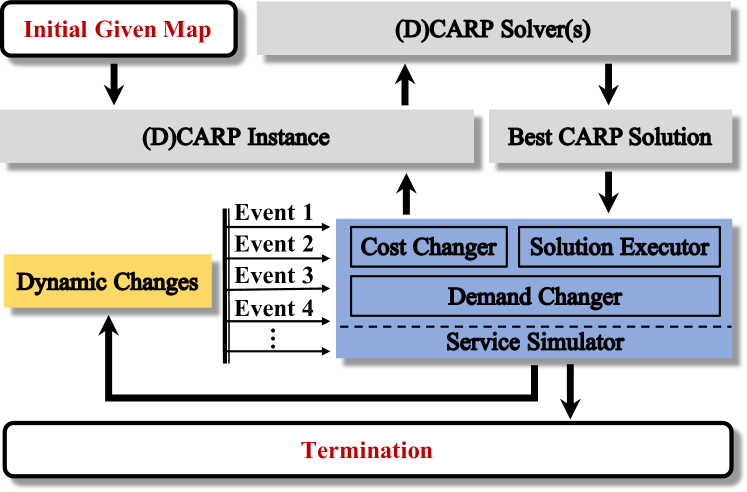
Figure 1: The architecture of our simulation system.

Input: Executable solution $S$, Previous instance $I_{m}$

Output: The new instance $I_{m+1}$

1 Set probabilities of occurrence for all events: $[p_{event},p_{road},p_{bdrr},p_{crr},p_{crbb},p_{icd},p_{add}]$;

2

3 Execute $S$ on $I_{m}$;

4 Select a uniformly random time to stop execution;

5 Remove all served tasks: make demand of all served tasks be $0$;

6 Event 1 Randomly select $n$ vehicles to break down.

7 /**** Cost Changer ****/

8

9for each arc $u_{i}\in A$ do

10      

11      if $rand()<p_{event}$ then

12             switch $state(u_{i})$ do

13                   case 0 do

14                         if $rand()<p_{road}$ then

15                               Event 2 $dc(u_{i})=\infty$, $state(u_{i})=2$

16                              

17                        else

18                               Event 3 $dc(u_{i})=\overline{dc(u_{i})}+c$, $state(u_{i})=3$

19                        

20                  

21                  case 2 do

22                         if $rand()>p_{bdrr}$ then

23                               Event 4 $dc(u_{i})=\overline{dc(u_{i})}$, $state(u_{i})=0$

24                        

25                  

26                  case 3 do

27                         $r=rand()$

28                         if $r<p_{crr}$ then

29                               Event 5 $dc(u_{i})=\overline{dc(u_{i})}$, $state(u_{i})=0$

30                         else if $r<p_{crbb}$ then

31                               Event 6 $dc(u_{i})=dc^{\prime}(u_{i})+c$

32                         else

33                               Event 7 $dc(u_{i})=dc^{\prime}(u_{i})-c$

34                        

35                  

36            

37      

38 /**** Demand Changer ****/

39 for each arc $u_{i}\in A$ do

40       if $dm(u_{i})>0$ and $rand()<p_{icd}$ then

41             Event 8 $dm(u_{i})=dm(u_{i})+d$

42      if $dm(u_{i})==0$ and $rand()<p_{add}$ then

43             Event 9 $dm(u_{i})=0+d$

44      

45

Algorithm 1 The pseudo code of the service simulator

In Figure 1, the system starts from a provided initial graph, which could be taken from existing benchmarks for static CARP. Then, a CARP solver selected by the user, such as solvers based on memetic algorithms [6], can be used to obtain the initial solution, i.e. the first schedule for the vehicles. The core part of the system is the Service Simulator in Figure 1, which is used to execute the CARP solution and update the graph. The pseudocode for the Service Simulator is presented in Algorithm 1. During the execution of the CARP solution, the maximum number of vehicles in the depot ($N_{veh}$) is considered. If the number of routes in the schedule exceeds the predefined maximum number of vehicles, the route with the smallest cost will be served first and the remaining routes will be served after some vehicles return to the depot. When the solution is executed, some dynamic events will happen according to a series of predefined parameters listed in Line 1 and influence the graph at a uniformly random time between the service start and completion time. After that, a new DCARP instance is generated based on the dispatched solution. Different solutions will result in different DCARP instances, which might not facilitate fair comparison of different algorithms. Therefore, we apply the best solution among all solutions obtained by different algorithms to the service simulator and generate one new DCARP instance for all algorithms for the fair comparison.

Once the dynamic change happens on the DCARP instance $I_{m}$, the Service Simulator stops the execution of the current solution. Then, the cost changer and demand changer will update the DCARP instance. First, as broken down vehicles influence only a specific arc, we simulate Event 1 separately from other dynamic events. The algorithm randomly selects $n$ vehicles from all dispatched vehicles to break down, as shown in Line 1. Events 2 to 7 will influence the cost of several arcs so that the cost changer mainly simulates these five events, as shown in Lines 1-1. Each arc $u_{i}$ has a traffic property, $state(u_{i})$, recording whether it is currently in a changed state compared to its original state having expected cost without traffic events.

In the cost changer, the simulator firstly determines whether or not a change from the current state occurs according to the probability $p_{event}$ for each arc. If a change occurs, a dynamic event is triggered according to the events’ probabilities and arc’s current changed state. If an arc keeps the original state, i.e. $state(u_{i})==0$, Event 2 or 3 happens in this arc depending on probability $p_{road}$. If $state(u_{i})==2$, the road has broken down before so that it recovers with a probability $p_{bdrr}$. If $state(u_{i})==3$, the road is in congestion. It may either completely recover with a probability $p_{crr}$, or the traffic jam may ease or get worse (by a random cost) with a probability $p_{crbb}$ or $1-p_{crbb}$, respectively. Compared to Events 2 to 7, Events 8 and 9 in the demand changer are much easier to implement, because we assume that the tasks/demands do not vanish unless served completely and the demand of tasks can only increase under the practical scenarios considered in this paper. Event 8 may happen to a task with a probability $p_{icd}$, increasing the demand by a random amount. For arcs with no demand, Event 9 will happen with a probability $p_{add}$.

Finally, we will get a new DCARP instance $I_{m+1}$, and the solver generates a new DCARP solution. The system terminates after all tasks are served.

IV A Generalised Optimisation Framework for DCARP

In this section, we propose a virtual-task strategy to change a DCARP instance to a ‘virtual static’ instance. After that, a generalised optimisation framework based on a virtual-task strategy for DCARP with two different initialisation strategies is proposed, which can make use of algorithms for static CARP for solving DCARP.

IV-A Virtual task

As discussed in the previous section, the main challenge of scheduling vehicles for DCARP by using algorithms designed for static CARP is to take the outside vehicles with different locations and remaining capacities into account. We propose a virtual task strategy that forces all outside vehicles to virtually return to the depot for optimisation purposes, such that all vehicles (some virtually) start at the depot during the optimisation. As a result, algorithms for static CARP, which assume that all vehicles start at the depot, can be adopted. After the optimisation, the obtained solution with routes starting from the depot will be converted to an executable solution according to the locations of outside vehicles. In other words, even though the outside vehicles will virtually return to the depot for running the optimisation process, in the executable solutions themselves, the outside vehicles start their new routes from their outside locations. For this strategy to work, some adjustments need to be made so that the optimisation problem with virtual tasks is equivalent to the actual DCARP instance being solved. Such adjustments will be explained next.

The pseudocode of constructing the virtual task is presented in Algorithm 2. Despite virtually returning to the depot, the outside vehicles are still required to start from the stop location when executing the new schedule after a change. So, these virtually returned vehicles have to first virtually move to their stop location in the new schedule. Therefore, the vehicles must serve some virtual paths in the new schedule to reach this stop location. The graph of the CARP instance is thus modified to include these virtual paths, which can be regarded as virtual tasks being optimised along with the normal tasks by a static CARP algorithm, as shown in Lines 2-2. We also need all vehicles in the depot to have the same full capacities to be able to use static CARP algorithms. Therefore, we assign the previous demands that have been served by an outside vehicle to the corresponding virtual task, as shown in Line 2. As a result, a DCARP instance is converted to a ‘static’ CARP instance, in which all vehicles are located at the depot with the same capacities. It is worthy to mention that the “virtual task” idea has also been used for large scale CARP [7], which is totally different from our idea here. They used the virtual task to represent the grouped neighboring tasks such that the problem’s dimensionality can be reduced.

Input: Task set $R=\{t_{1},t_{2},...,t_{N_{t}}\}$,
Stop locations of outside vehicles: $OV$,
Remaining capacity of outside vehicles: $RQ$.
$OV=\{v_{1},v_{2},...,v_{N_{ov}}\}$, $RQ=\{q_{1},q_{2},...,q_{N_{ov}}\}$

Output: The updated task set: $R$

1 for each outside vehicle $k$ do

2       Construct an Arc with virtual task $vt_{k}$;

3       Head: $head_{vt_{k}}$ = $v_{0}$, where $v_{0}$ is the depot;

4       Tail: $tail_{vt_{k}}$ = $v_{k}$;

5       Deadheading cost: $dc(vt_{k})$ = $\infty$;

6       Serving cost: $sc(vt_{k})$ = $mdc(v_{0},v_{k})$;

7       Demand: $dm(vt_{k})$ = $Q-q_{k}$, where $Q$ is the original capacity of vehicles;

8       Add this virtual task into task set: $R=R\cup vt_{k}$.

Algorithm 2 Pseudocode of constructing virtual tasks

A virtual task can also be interpreted as a representation of an outside vehicle’s previous serving status, including the total cost, served demand and stop location before the occurrence of the dynamic events. During the optimisation, the virtual tasks are regarded as arcs to be assigned to routes when being rescheduled. These arcs need to be served, so that some depot vehicles will actually correspond to the outside vehicles. Once a depot vehicle serves a virtual task, its remaining capacity will become the same as the remaining capacity of the corresponding outside vehicle, and so will its stop location. However, vehicles that are not serving these virtual arcs should not be able to traverse them, because these virtual arcs are not actual physical paths that can be used by vehicles. This is achieved by assigning a deadheading cost (traversing cost) of $dc(vt)=\infty$ to these arcs, as shown in Line 2. Note that this infinite traversing cost is not included as part of the serving cost.

The serving cost of a virtual task should be zero. This is because in reality, the outside vehicles are already in the stop locations and have already served some tasks. They should not incur any extra cost to stay where they were. However, in our strategy, a virtual task’s serving cost is set as the minimal total deadheading cost between the depot and the vehicle stop location (Line 2) because some algorithms such as Path-Scanning use this cost as a denominator when deciding which task to assign to the current route [4]. To avoid this cost being counted towards the total cost in the objective function, the additional cost will be subtracted from the actual total cost after the optimisation using the virtual task strategy. Besides, the demand is set as the amount corresponding to the demand already served by the vehicle, i.e. $Q-q_{k}$, to avoid the total demand of tasks in its new route exceeding the vehicle’s remaining capacity $q_{k}$ (Line 2).

In order to improve the understanding of how virtual tasks in DCARP instances are constructed, an example for tasks $t_{1},t_{2}$ is provided in Figure 2. One vehicle traverses from $v_{0}$ (depot) and serves the task $t_{1}$ (Figure 2 left). When the dynamic change happens, a vehicle is located at $v_{2}$. This vehicle is virtually placed into the depot and a virtual task $vt_{1}$ is constructed between $v_{0}$ and $v_{2}$ (Figure 2 right). This virtual task will enable the vehicle to go back to its outside position to continue serving other tasks. The demand of $vt_{1}$, $dm(vt_{1})$, equals to $Q-dm(t_{1})$, such that when the vehicle virtually returns to its outside position, its remaining capacity will be the same as the remaining capacity at the rescheduling point. The deadheading cost of $vt_{1}$, $dc(vt_{1})$ is set to $\infty$ to prevent other vehicles from traversing the virtual arc. This enables the outside vehicle to serve the virtual task. The serving cost of $vt_{1}$, $sc(vt_{1})$, equals to $mdc(v_{0},v_{2})$. This serving cost is incurred by the vehicle when it serves the virtual task, but is later on deducted from the objective function of the problem, so that the objective value with the virtual task strategy remains the same as the objective value without the virtual task strategy. After that, the new DCARP instance with the remaining task $t_{2}$ and the virtual task $vt_{1}$ will be optimised using one of the algorithms which are available for static CARP, in which the task $t_{1}$ is removed because it was already served before the change that triggered the rescheduling.

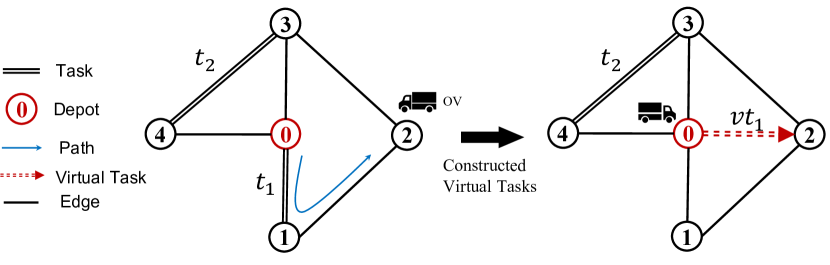
Figure 2: An example of constructing virtual tasks.

After applying the virtual-task strategy, the route formulation in a DCARP solution $S=\{r_{1},r_{2},...,r_{N_{ov}},...,r_{K}\}$ becomes:

$$r_{k}={\color[rgb]{0,0,0}(}v_{0},vt_{k},t_{k,2},t_{k,3},...,t_{k,l_{k}},v_{0}{\color[rgb]{0,0,0})},k=1,2,...,N_{ov}.$$

$$r_{k}={\color[rgb]{0,0,0}(}v_{0},t_{k,1},t_{k,2},...,t_{k,l_{k}},v_{0}{\color[rgb]{0,0,0})},k=N_{ov}+1,...,K.$$

The new formulation of the optimisation objective and the constraints for a DCARP instance is given in Eq. 3:

$$\mathbf{Min} \quad TC(S)=\sum_{k=1}^{K}RC_{r_{k}}-\sum_{k=1}^{N_{ov}}mdc(v_{0},v_{k}).$$ (3)

$$\mathbf{s.t.} \quad\sum_{k=1}^{K}l_{k}=N_{t}+N_{ov}.$$

$$\quad t_{k_{1},i_{1}}\neq t_{k_{2},i_{2}},{\color[rgb]{0,0,0}\mathrm{for\ all\ }}(k_{1},i_{1})\neq(k_{2},i_{2}).$$

$$\quad\sum_{i=1}^{l_{k}}dm(t_{k,i})\leq Q,\forall k=1,...,K.$$

where for route $\{r_{k}|k=1,2,...,N_{ov}\}$, $t_{k,1}=vt_{k}$. The second term $\sum_{k=1}^{N_{ov}}mdc(v_{0},v_{k})$ is to balance out Line 2 in Algorithm 2 so that we do not count the serving costs of virtual tasks.

The above adjustments enable a new schedule for the converted ‘static’ CARP instance to be obtained by directly using meta-heuristic algorithms for static CARP. An executable solution is obtained by removing the virtual tasks from the routes in the new schedule and assigning it to the corresponding outside vehicles. The virtual task is better to be the first task in a vehicle’s route. If a given virtual task is not the first task of a service route found by the static CARP algorithm, the tasks before this virtual task will be assigned to a new vehicle starting from the depot and the following tasks will be served by the corresponding outside vehicle. In such a case, we split a route that contains virtual tasks in the middle into multiple routes with one route served by a vehicle from the depot and others served by the corresponding outside vehicle. In this way, the total cost of the CARP solution will not be influenced by splitting because the head node of the virtual task is also the depot. An example (without relations to Figure 2) of converting an obtained new solution to an executable service plan is provided below:

$$\begin{array}[]{c}{\color[rgb]{0,0,0}(v_{0},vt_{1},t_{2},v_{0}),(v_{0},t_{3},t_{4},vt_{2},t_{5},v_{0})}\\ \downarrow\\ {\color[rgb]{0,0,0}(v_{0},vt_{1},t_{2},v_{0}),(v_{0},t_{3},t_{4},v_{0}),(v_{0},vt_{2},t_{5},v_{0})}\\ \downarrow\\ {\color[rgb]{0,0,0}(v_{1},t_{2},v_{0}),(v_{0},t_{3},t_{4},v_{0}),(v_{2},t_{5},v_{0})}.\end{array}$$

In the above example, the solution (top) contains two routes and two outside vehicles (i.e. two virtual tasks). In the second route, the virtual task located in the middle of the task sequence. If the first task of a route is a virtual task, the remaining tasks of the route are served by the outside vehicle. Otherwise, all tasks of the route are served by a new empty vehicle. Therefore, after conversion (middle), tasks $t_{3},t_{4}$ are assigned to a new vehicle starting from the depot, but task $t_{5}$ should actually be served by the outside vehicle. The final executable routes (bottom), are obtained by removing the virtual tasks and starting from the corresponding stop locations (The $v_{1}$ and $v_{2}$ are the stop locations of outside vehicles corresponding to $vt_{1}$ and $vt_{2}$).

IV-B Proposed Framework based on Virtual-Task Strategy

There are generally two commonly used strategies in dynamic optimisation. One is to re-start the optimisation, which can also include some additional diversity enhancing techniques [28]. The other is to migrate some good solutions for the old environment to the new environment and initialise the starting individuals with them [29, 30].

These two strategies could also be used in our optimisation framework. The restart strategy is straightforward to apply after a change has occurred. However, the current strategies for re-using good solutions for the old environment may not be suitable for our DCARP scenarios because the dynamic events may influence the problem’s dimension and the previous solution’s feasibility in a DCARP scenario. For example, the served tasks and added tasks change the total number of tasks, and the potential road closure event makes previous solutions infeasible in the new DCARP instance.

Therefore, we propose a new knowledge (especially sequence) transfer strategy for the DCARP scenario (Algorithm 3), which can benefit from previous DCARP instance’s best solutions. Given an instance $I_{m}$, all scheduled routes in the best solution $S_{m-1}$ of the previous instance $I_{m-1}$ are concatenated to construct an ordered list of tasks $P_{m-1}$. All tasks that have been served are then removed from the list in $P_{m-1}$, and the remaining tasks keep their orders. After that, the newly added tasks are inserted into $P_{m-1}$ greedily, i.e., they are inserted into the positions with the smallest increased cost. Finally, a corresponding transferred solution is generated by using the split scheme to convert an ordered list to an explicit-route solution. The newly transferred solution is used as one of the initial solutions when optimising the new DCARP instance using the population-based algorithm.

Input: Previous best solution $S_{m-1}$

Output: A newly transferred solution $S_{m}$

1 Convert $S_{m-1}$ into an ordered list of tasks $P_{m-1}$;

2 Remove all served tasks from $P_{m-1}$;

3 $P_{m}=P_{m-1}$, $l_{P}=|P_{m}|$;

4 The newly added tasks set $NT=\{nt_{1},nt_{2},...,nt_{|NT|}\}$;

5 for each $nt_{i}\in NT$ do

6       for each position in $P_{m}$ do

7             Calculate the increased cost after insertion;

8      Obtain the position $p$ with the smallest increased cost;

9       Insertion: $P_{m}=[t_{1},...,t_{p},nt_{i},t_{p+1},...,t_{l_{P}}]$;

10       $l_{P}=l_{P}+1$;

11       $NT=NT\setminus\{nt_{i}\}$.

12      

13

14Use split scheme in $P_{m}$.

15

Algorithm 3 Pseudocode of knowledge (sequence) transfer strategy

On the basis of the virtual-task strategy and two initialisation strategies, i.e. the restart strategy and the sequence transfer strategy, we propose a generalised optimisation framework with virtual tasks (GOFVT) to generalise static CARP algorithms to dynamic scenarios. Our framework comprises four main steps:

1. Construct virtual tasks;

2. Apply the restart strategy (randomly generate initial solutions) or the sequence transfer strategy (generate one transferred solution for individual-based algorithms and additionally generated random solutions for population-based algorithms);

3. Apply the meta-heuristic algorithm to optimize the converted “static” CARP instance;

4. Convert the obtained solution with virtual tasks to an executable solution without virtual tasks.

For a DCARP instance, the framework will first construct the virtual tasks to convert the dynamic instance to a ‘static’ instance. Then, one of the two initialisation strategies explained above can be adopted to assist the optimisation for the DCARP instance. In the computational studies in Section V, we will compare the effectiveness of these two strategies. Then, meta-heuristic algorithms with the initialisation strategy are applied to optimise the DCARP instance which is a ‘static’ instance with virtual tasks. Finally, the solution obtained for the ‘static’ instance is converted into an executable solution, in which the routes with virtual tasks are assigned to the corresponding outside vehicles and the routes without virtual tasks are assigned to vehicles located at the depot.

V Computational Studies

In order to evaluate the efficiency of our proposed framework (GOFVT), three sets of experimental studies have been conducted by embedding a selection of meta-heuristic algorithms in the GOFVT in this section. After providing the experimental set-up (Section V-A), in the first experiment, the virtual-task strategy is compared with a simple rescheduling strategy (Section V-B). After that, the virtual-task strategy’s efficiency is investigated by comparing it with an existing algorithm for DCARP in the second experiment (Section V-C). Finally, in the last experiment, GOFVT is combined with several classical meta-heuristic algorithms originally designed for static CARP, and its performance is analysed by running the newly generated algorithms in DCARP scenarios (Section V-D).

V-A Experimental Settings

All experiments are conducted on a series of DCARP instances or scenarios generated by the simulation system presented in Section III-B, based on a static CARP benchmark, namely the egl set [31]. The egl set contains 24 CARP instances. In each experiment, the DCARP instances or scenarios are generated independently from static CARP instances. For our first and second set of experiments, 3 DCARP instances are generated for each static CARP instance. These DCARP instances are not used to compose a DCARP scenario, as the algorithms just optimise the current instance and do not use any knowledge transfer in these two experiments. For the third experiment, one DCARP scenario including 5 DCARP instances is generated based on each CARP instance. For a fair comparison, each DCARP instance is generated from the best solution among all obtained solutions by all compared algorithms in the previous instance. When the simulator executes the selected solution according to the deployment policy, the time for serving all tasks will be calculated first and the simulator will uniformly randomly select a stop point (for dynamic events) within the longest time. As we only requires a set of DCARP instances to test the effectiveness of proposed strategies and framework, we have arbitrarily chosen parameters according to real world situations. For example, a road is more likely to become congested than being closed, hence we set $p_{road}=0.1$. In our experiments, the parameters of the simulator are chosen as $p_{event}=0.5$, $p_{road}=0.1$, $p_{bdrr}=0.5$, $p_{crr}=0.3$, $p_{crbb}=0.6$, $p_{cid}=0.35$, $p_{add}=0.35$. In the future, we will carry out a more comprehensive study of the characteristics of simulator in relation to its parameter values. Eight different types of dynamic changes (Table II) are simulated in our simulator excluding the case of “vehicles broken down” because its formulation is the same as the event of added tasks. As an illustrative example, we investigate the influence of different scenarios on the optimisation algorithms’ performances. These examples show that the scenario with newly added tasks has a significant influence on the optimisation algorithm’s performance.

Because a key optimisation requirement when dynamic changes happen in the real world is to obtain a new solution quickly, we limit the maximum optimisation time to 60s for the small problems (E1 $\sim$ E4) and 180s for larger maps (S1 $\sim$ S4) in egl for all algorithms. All programs are implemented in C language and run using a PC with an Intel Core i7-8700 3.2GHZ. The source code of our experiments has been available on github.

V-B Is It Necessary to Reschedule for DCARP?

Although many algorithms have been proposed to solve DCARP in the literature, a simple baseline strategy, named the return-first strategy, has been ignored. The return-first strategy schedules all outside vehicles back to the depot first in order to convert a DCARP instance to a static one, and then reschedules all vehicles for the new static instance after all vehicles are located at the depot. If the return-first strategy is efficient enough, the direct optimisation of a DCARP instance would not be necessary any more. However, since this has not been shown in the literature so far, in this subsection, we use the proposed virtual-task strategy to solve DCARP and compare it with the return-first strategy to show the importance of optimising DCARP instances directly instead of ignoring the outside vehicles and assigning new vehicles to all remaining tasks.

TABLE III: Results of virtual-task strategy (VT) and return-first strategy (RF) on DCARP instances with different settings of remaining capacities from the egl dataset. The value in each cell represents “Mean $\pm$ Std” over 25 independent runs and the bold ones denote the better result on the DCARP instance based on the Wilcoxon signed-rank test with a significance level of 0.05. The penultimate row summaries the number of win-draw-lose of RF strategy versus VT strategy and the last row provides the p-values of the Wilcoxon signed-rank test with a significance level of 0.05 on instances with the same settings of all maps.

Static Map Instance 1 ($q\in[0,0.33Q]$) Instance 2 ($q\in[0.34Q,0.66Q]$) Instance 3 ($q\in[0.67Q,Q]$) RF VT RF VT RF VT E1-A 8386$\pm$22 8095$\pm$31 10397$\pm$34 9925$\pm$22 8630$\pm$8 8566$\pm$10 E1-B 9830$\pm$29 9839$\pm$39 9718$\pm$22 8437$\pm$28 9675$\pm$16 9208$\pm$29 E1-C 12181$\pm$52 12109$\pm$52 14726$\pm$31 14106$\pm$16 11286$\pm$11 10565$\pm$25 E2-A 10255$\pm$6 10480$\pm$6 13740$\pm$27 12278$\pm$29 11692$\pm$51 10231$\pm$34 E2-B 13162$\pm$15 13317$\pm$23 16435$\pm$29 15207$\pm$18 15667$\pm$35 14321$\pm$55 E2-C 17425$\pm$41 17566$\pm$35 17444$\pm$32 16881$\pm$25 14186$\pm$16 13871$\pm$46 E3-A 11343$\pm$42 11167$\pm$17 12877$\pm$21 12030$\pm$26 10369$\pm$19 8869$\pm$12 E3-B 15517$\pm$84 15776$\pm$31 15150$\pm$31 12797$\pm$68 20743$\pm$59 20081$\pm$39 E3-C 20549$\pm$69 20880$\pm$63 20012$\pm$144 18078$\pm$88 27521$\pm$81 25289$\pm$82 E4-A 11216$\pm$31 11387$\pm$27 12489$\pm$26 12152$\pm$32 16213$\pm$29 14858$\pm$135 E4-B 15522$\pm$40 15242$\pm$62 14933$\pm$65 13791$\pm$63 17477$\pm$71 15869$\pm$29 E4-C 20928$\pm$63 20691$\pm$41 21998$\pm$28 20174$\pm$86 17869$\pm$79 15798$\pm$59 S1-A 16097$\pm$49 16012$\pm$40 15643$\pm$31 14917$\pm$40 13684$\pm$53 13159$\pm$18 S1-B 20462$\pm$69 21167$\pm$58 16184$\pm$35 15697$\pm$35 15151$\pm$19 13428$\pm$82 S1-C 27944$\pm$71 28624$\pm$116 21040$\pm$36 18616$\pm$87 26470$\pm$103 25789$\pm$76 S2-A 19610$\pm$85 19479$\pm$107 22314$\pm$40 20016$\pm$48 22499$\pm$67 19212$\pm$82 S2-B 27970$\pm$75 28408$\pm$59 26334$\pm$130 25911$\pm$118 25723$\pm$67 25024$\pm$94 S2-C 31859$\pm$108 32101$\pm$125 40170$\pm$132 38575$\pm$186 35053$\pm$143 31815$\pm$133 S3-A 19489$\pm$64 19211$\pm$107 23630$\pm$118 21329$\pm$98 28237$\pm$76 24494$\pm$71 S3-B 27518$\pm$72 27521$\pm$98 25651$\pm$64 24311$\pm$93 32286$\pm$50 30646$\pm$96 S3-C 32468$\pm$93 32049$\pm$107 35435$\pm$67 33927$\pm$68 43151$\pm$98 40801$\pm$97 S4-A 27256$\pm$87 28082$\pm$142 23780$\pm$74 22788$\pm$95 29895$\pm$102 27576$\pm$105 S4-B 34872$\pm$122 34709$\pm$149 28283$\pm$121 28023$\pm$93 31770$\pm$87 30652$\pm$125 S4-C 43746$\pm$168 44165$\pm$157 36808$\pm$117 36706$\pm$123 44006$\pm$145 42827$\pm$178 $\#$of ‘w-d-l’ 12-3-9 0-0-24 0-0-24 p-value 0.22 1.82e-5 1.82e-5

TABLE IV: Results of MASDC and VT-MASDC on DCARP instances from the egl dataset. The value in each cell represents “Mean $\pm$ Std” over 25 independent runs and the bold ones denote the better result on the DCARP instance based on the Wilcoxon signed-rank test with a significance level of 0.05. The last row summaries the number of win-draw-lose of MASDC versus VT-MASDC.

Map	Ins.Index	MASDC	VT-MASDC
S4-A	1	58456$\pm$1621	51512$\pm$3298
	2	55394$\pm$1746	49422$\pm$3517
	3	64795$\pm$1546	58676$\pm$3517
S4-B	1	64343$\pm$1886	57017$\pm$3622
	2	65027$\pm$1712	57413$\pm$3033
	3	60143$\pm$1612	53342$\pm$3323
S4-C	1	69224$\pm$1475	62760$\pm$2929
	2	68070$\pm$1424	62304$\pm$2465
	3	78134$\pm$1893	69348$\pm$3451
Statistical results over 72 instances below
$\#$ of win-draw-lose			0-0-72
p-value			1.67e-13

• The data of E1-A $\sim$ S3-C are omitted in the table due to the page limitation. The complete data are provided in the supplementary material.

In our experiment, the simulation system generates three different DCARP instances for each test map (i.e., a static instance in the egl benchmark set) with different sets of remaining capacities. As this experiment aims to demonstrate the necessity and efficiency of directly optimising DCARP instances, the setting of remaining capacities is divided into three intervals, i.e., $[0,0.33Q]$, $[0.34Q,0.66Q]$ and $[0.67Q,Q]$. Then, an optimisation algorithm, Memetic Algorithm with Extended Neighborhood Search (MAENS) [6], assisted with the return-first strategy and virtual-task strategy are applied to optimise each DCARP instance, respectively. Two algorithm instantiations using MAENS follow the same setting during the optimisation that the return-first strategy and virtual-task strategy is the only difference between them. The comparison results in terms of mean and standard deviation over 25 independent runs (mean$\pm$std), of the return-first (RF) strategy and virtual-task (VT) strategy on DCARP instances with different remaining capacities are presented in Table III. The bold values with grey background for each DCARP instance are the better results between return-first strategy and virtual-task strategy based on the Wilcoxon signed-rank test with a significance level of 0.05. The second last row of Table III summarises the number of win-draw-lose of the RF versus VT strategies. We have calculated the Wilcoxon signed-rank test with a significance level of 0.05 for the mean total cost of RF and VT strategies on the instances with the same range of remaining capacities, and the p-values are listed in the last row of Table III.

Table III shows that the RF and VT strategies are significantly different for the instances where the remaining capacities are in the range of $[0.34Q,Q]$ (instances 2 and 3 in Table III), with the VT strategy outperforming the RF strategy on all DCARP instances. In contrast, for the scenarios with remaining capacities in $[0,0.33Q]$, there are 12 out of 24 DCARP instances where the RF strategy outperforms the VT strategy. When comparing the results using the Wilcoxon test across maps, we confirm that none of these strategies is a consistent winner when analysed across maps where the remaining capacities are smaller than $0.33Q$. This is understandable because when the vehicles are mostly fully loaded, i.e., when the remaining capacities are smaller than 0.33Q, there is limited space for serving more tasks no matter what strategy is used.

In order to avoid the conclusion being biased by the employed meta-heuristic algorithm, we have employed another meta-heuristic algorithm, i.e., ILMA [32], to execute the same experiment. Due to the page limitation, we put the results into Table V of the supplementary material. The statistical analysis has confirmed the same conclusion as the experiments employing MAENS.

Overall, we can conclude that it is necessary and much more effective to optimise the DCARP instance directly rather than using the RF strategy when outside vehicles have enough remaining capacities.

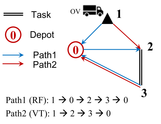
Figure 3: An example of demonstrating why the RF strategy is not efficient enough when outside vehicles have enough remaining capacities.

The reason why the RF strategy is not always helpful when outside vehicles have enough remaining capacities can be explained using a simple example in Figure 3, where an outside vehicle stops at vertex 1. If its remaining capacity is sufficient to serve task $t_{23}$, it can directly traverse from vertex 1 to vertex 2, presented as ‘Path 2’ in Figure 3, and the final total cost will be $d_{vt}=d_{12}+d_{23}+d_{30}$. But if we apply the RF strategy, the total cost will change to $d_{rf}=d_{10}+d_{02}+d_{23}+d_{30}$, presented as ‘Path 1’ in Figure 3. It is obvious that $d_{rf}\geq d_{vt}$ because $d_{10}+d_{02}\geq d_{12}$ according to triangle inequality. The RF strategy increases the final cost because vehicles take a detour in such cases.

V-C Analysis of the Effects of the Virtual-Task Strategy

Memetic algorithm with new split scheme (MASDC) [16] is the only meta-heuristic algorithm for DCARP in the literature that considers a general DCARP scenario including several dynamic events, such as road closure and added tasks. It comprises a distance-based split scheme to assist the DCARP solution being used in the crossover and local search. Our virtual-task strategy can convert a DCARP instance to a ‘static’ CARP instance so that the operator used in the static CARP can be used in the DCARP instance directly. In this subsection, we analyse the effects of our VT strategy by embedding it to MASDC, referred to as VT-MASDC, and comparing it to the original MASDC. The advantage of embedding our strategy into MASDC is that this enables us to isolate and analyse the effect of the virtual tasks compared to a state-of-the-art DCARP algorithm. In particular, all components in MASDC and VT-MASDC are the same except for the use of virtual tasks and the distance-based split scheme. The latter needs to be replaced by Ulusoy’s split scheme in VT-MASDC because the distance-based split scheme is specifically designed for DCARP instances with outside vehicles at different stop locations. When we apply the virtual task strategy, the DCARP instance is converted to the ‘static’ instance where all vehicles are located at the depot. Therefore, the distance-based split scheme is not suitable anymore and the Ulusoy’s split scheme is used instead. The use of virtual tasks is thus inherently linked to this split scheme, and any advantages provided by the virtual tasks are also linked to the fact that they enable this split scheme to be adopted.

In our experiment, we generate three independent DCARP instances for each map in the egl benchmark set, ensuring that outside vehicles has enough remaining capacities, i.e. $q\geq 0.5Q$, in all generated instances. However, we need to generate DCARP instances rather than DCARP scenarios because the aim of DCARP is to minimise the total cost for each DCARP instance separately (Eq. 2). The optimisation results are presented in Table IV, in which the values in each cell represent the mean and standard deviation over 25 independent runs (mean$\pm$std). For each DCARP instance, the better result, based on the Wilcoxon signed-rank test with a significance level of 0.05, is highlighted using a bold font and grey background in Table IV. The summary of win-draw-lose of MASDC versus VT-MASDC, which is presented in the last row, shows that VT-MASDC outperforms MASDC on all generated DCARP instances. The Wilcoxon signed-rank test with a significance level of 0.05 was conducted for the average total cost of VT-MASDC and MASDC in all instances, and the p-value was 1.67e-13. Overall, we can conclude that VT-MASDC performs much better than the original MASDC.

MASDC uses a distance-based split scheme (DSS) to evaluate DCARP solution’s fitness because the split scheme designed for static CARP is not suitable for DCARP [25]. The DSS operator randomly splits the sequence of tasks to an executable CARP solution with explicit routes, and the random splitting process is repeated three times to obtain a better schedule. After embedding with the VT strategy, the DSS operator is replaced by Ulusoy’s split [3] as explained in the beginning of this subsection, and the evaluation of a sequence of tasks only requires to apply the Ulusoy’s split once. As a result, the randomness brought by the DSS’s split scheme is removed.

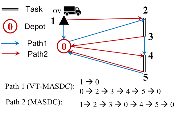
Figure 4: An example of demonstrating the advantages of considering new vehicles.

Moreover, the DSS operator never considers new vehicles starting from the depot during the optimisation, whereas our VT strategy enables both outside and new vehicles to be used. We provide an example in Figure 4 to show the advantages of considering new vehicles during the optimisation of DCARP. An outside vehicle is located at vertex 1, and its remaining capacity can only serve task $t_{23}$. We assume that $dd_{10}+dd_{02}\approx dd_{12}$ and $dd_{30}+dd_{04}\gg dd_{34}$ and the total cost of ‘Path1’ and ‘Path2’ can be calculated as:

$$\begin{array}[]{c}TC_{1}=\underline{{\color[rgb]{0,0,0}dd_{10}}+dd_{02}}+sc_{23}+\underline{dd_{34}}+sc_{45}+dd_{50},\\ TC_{2}=\underline{dd_{12}}+sc_{23}+\underline{dd_{30}+dd_{04}}+sc_{45}+dd_{50}.\\ \end{array}$$

For a sequence of tasks $[0,t_{23},t_{45},0]$, if applied with the DSS operator, the only obtained path will be ‘Path 2’ as shown in Figure 4. In contrast, if we use the VT strategy, a better path, i.e. ‘Path 1’ in Figure 4, can be obtained, which avoids traversing the longer returning path.

TABLE V: Results of VT-RTS, VTtr-RTS, VT-ILMA, VTtr-ILMA, VT-MAENS, VTtr-MAENS, VT-MASDC and VTtr-MASDC on the egl dataset. The values in each cell represent the “MEAN$\pm$STD” with the average ranking (in the brackets) w.r.t the average total cost over 25 independent runs. The bold values are the better results under the Wilcoxon signed-rank test with a significance level of 0.05 between restart and inheriting strategies in an algorithm for a DCARP instance. The last three rows summarise the number of win-draw-lose of restart strategy versus inheriting strategy in each algorithm and the p-values of the Wilcoxon signed-rank test with a significance level of 0.05 on all instances.

Map Ins.Index VT-RTS VTtr-RTS VT-ILMA VTtr-ILMA VT-MAENS VTtr-MAENS VT-MASDC VTtr-MASDC S3-A 1 22989$\pm$156(3.6) 22971$\pm$190(3.4) 24100$\pm$307(5.5) 24073$\pm$289(5.5) 22411$\pm$61(1.5) 22401$\pm$70(1.5) 52327$\pm$3849(7.5) 52327$\pm$3849(7.5) 2 25249$\pm$348(2.5) 26012$\pm$192(4.0) 27134$\pm$338(5.3) 27234$\pm$405(5.6) 25013$\pm$105(1.8) 25017$\pm$103(1.8) 57870$\pm$3931(7.5) 57870$\pm$3931(7.5) 3 25907$\pm$350(3.3) 26117$\pm$160(3.7) 27011$\pm$250(5.5) 27042$\pm$320(5.5) 25285$\pm$145(1.4) 25349$\pm$113(1.6) 59652$\pm$3792(7.5) 59652$\pm$3792(7.5) 4 41928$\pm$177(6) 33347$\pm$287(3) 34800$\pm$398(4.5) 34840$\pm$420(4.5) 32374$\pm$119(1.4) 32423$\pm$100(1.6) 72252$\pm$4788(7.5) 72250$\pm$4790(7.5) 5 31319$\pm$4(6) 24329$\pm$316(2.7) 25614$\pm$322(4.6) 25632$\pm$334(4.4) 23989$\pm$74(1.7) 24006$\pm$85(1.6) 62362$\pm$4014(7.5) 62362$\pm$4014(7.5) S3-B 1 30945$\pm$70(6) 29429$\pm$141(5) 26486$\pm$282(3.4) 26493$\pm$230(3.6) 25161$\pm$123(1.5) 25165$\pm$106(1.5) 46491$\pm$3247(7.5) 46491$\pm$3247(7.5) 2 28494$\pm$1307(3.5) 29198$\pm$1867(4.1) 29318$\pm$356(5.2) 29374$\pm$347(5.2) 27445$\pm$121(1.8) 27356$\pm$140(1.2) 55642$\pm$2518(7.5) 55642$\pm$2518(7.5) 3 36665$\pm$2093(5.3) 35529$\pm$3448(3.8) 34378$\pm$330(4.2) 34515$\pm$347(4.7) 32584$\pm$78(1.5) 32613$\pm$112(1.5) 65559$\pm$3265(7.5) 65559$\pm$3265(7.5) 4 36424$\pm$10(6) 29498$\pm$240(3.0) 30262$\pm$280(4.6) 30306$\pm$339(4.4) 28983$\pm$133(1.6) 28930$\pm$131(1.4) 59740$\pm$4565(7.5) 59740$\pm$4565(7.5) 5 32715$\pm$2377(4.0) 31524$\pm$348(3.7) 32271$\pm$345(5.2) 32185$\pm$417(5.1) 30444$\pm$167(1.4) 30437$\pm$160(1.6) 61165$\pm$3506(7.5) 61165$\pm$3506(7.5) S3-C 1 45906$\pm$0(5.0) 47919$\pm$1147(6.0) 40932$\pm$333(3.4) 40930$\pm$425(3.6) 39026$\pm$146(1.4) 39049$\pm$154(1.6) 69270$\pm$3741(7.5) 69270$\pm$3741(7.5) 2 58082$\pm$263(5.0) 58770$\pm$195(6.0) 51538$\pm$346(3.6) 51445$\pm$366(3.4) 49131$\pm$169(1.5) 49157$\pm$207(1.5) 78938$\pm$4233(7.5) 78938$\pm$4233(7.5) 3 45802$\pm$74(5.2) 45868$\pm$21(5.8) 38727$\pm$341(3.4) 38925$\pm$241(3.6) 36791$\pm$118(1.6) 36730$\pm$94(1.4) 67602$\pm$3362(7.5) 67602$\pm$3362(7.5) 4 41011$\pm$1(6) 40879$\pm$115(5) 35457$\pm$319(3.5) 35339$\pm$338(3.5) 33663$\pm$89(1.7) 33653$\pm$91(1.3) 61607$\pm$2949(7.5) 61607$\pm$2949(7.5) 5 49309$\pm$114(5.5) 46793$\pm$3817(4.8) 42843$\pm$488(3.9) 42764$\pm$568(3.7) 40153$\pm$107(1.6) 40143$\pm$132(1.4) 72621$\pm$3858(7.5) 72621$\pm$3858(7.5) S4-A 1 24849$\pm$1470(6) 21105$\pm$170(2.9) 22336$\pm$255(4.5) 22385$\pm$332(4.5) 20730$\pm$131(1.6) 20699$\pm$85(1.5) 53513$\pm$3603(7.5) 53513$\pm$3603(7.5) 2 24693$\pm$1073(3.1) 24947$\pm$322(4.0) 26177$\pm$477(5.4) 26175$\pm$352(5.5) 23967$\pm$134(1.6) 23920$\pm$96(1.4) 59023$\pm$3019(7.5) 59020$\pm$3023(7.5) 3 28262$\pm$12(6) 22203$\pm$286(3) 23181$\pm$356(4.4) 23091$\pm$319(4.5) 21661$\pm$67(1.6) 21638$\pm$68(1.4) 49301$\pm$3606(7.5) 49325$\pm$3575(7.5) 4 28294$\pm$261(4.6) 27786$\pm$653(3.1) 28551$\pm$420(5.0) 28636$\pm$379(5.4) 26885$\pm$82(1.7) 26856$\pm$103(1.3) 62334$\pm$3972(7.5) 62334$\pm$3972(7.5) 5 28727$\pm$249(3.0) 28989$\pm$389(3.6) 30571$\pm$479(5.5) 30693$\pm$441(5.5) 28421$\pm$139(1.6) 28440$\pm$125(1.8) 64233$\pm$5147(7.5) 64242$\pm$5138(7.5) S4-B 1 47887$\pm$173(6) 40827$\pm$2573(3.3) 41301$\pm$476(4.4) 41242$\pm$464(4.3) 38564$\pm$117(1.6) 38549$\pm$139(1.4) 70139$\pm$4037(7.5) 70144$\pm$4029(7.5) 2 43677$\pm$0(5.6) 43024$\pm$2961(4.7) 40667$\pm$448(3.7) 40804$\pm$492(4.0) 38055$\pm$128(1.5) 38061$\pm$172(1.5) 70219$\pm$3947(7.5) 70219$\pm$3947(7.5) 3 50458$\pm$193(3.4) 50440$\pm$239(3.2) 52701$\pm$547(5.6) 52632$\pm$519(5.4) 50091$\pm$210(1.6) 50103$\pm$151(1.8) 83768$\pm$3444(7.5) 83768$\pm$3444(7.5) 4 34946$\pm$288(5.6) 33974$\pm$1347(3.2) 34526$\pm$317(4.4) 34478$\pm$318(4.7) 32820$\pm$95(1.5) 32864$\pm$148(1.5) 62765$\pm$3949(7.5) 62765$\pm$3949(7.5) 5 38698$\pm$4308(4.5) 38901$\pm$3107(4.8) 36166$\pm$349(4.4) 36195$\pm$289(4.4) 34049$\pm$163(1.6) 34016$\pm$143(1.4) 65365$\pm$4152(7.5) 65369$\pm$4147(7.5) S4-C 1 42365$\pm$10(5.7) 42128$\pm$314(5.3) 35903$\pm$393(3.5) 35922$\pm$456(3.5) 33866$\pm$168(1.5) 33892$\pm$143(1.5) 61633$\pm$3417(7.5) 61633$\pm$3417(7.5) 2 49614$\pm$26(5) 49797$\pm$74(6) 44052$\pm$394(3.4) 44087$\pm$340(3.6) 41842$\pm$170(1.4) 41878$\pm$204(1.6) 71240$\pm$3779(7.5) 71240$\pm$3779(7.5) 3 50103$\pm$0(6) 49263$\pm$282(5) 41426$\pm$369(3.6) 41299$\pm$442(3.4) 39367$\pm$173(1.4) 39386$\pm$133(1.6) 71625$\pm$2776(7.5) 71625$\pm$2776(7.5) 4 51311$\pm$0(6) 50781$\pm$48(5) 44940$\pm$369(3.4) 45099$\pm$410(3.6) 42895$\pm$168(1.4) 42939$\pm$179(1.6) 72347$\pm$3396(7.5) 72347$\pm$3396(7.5) 5 46067$\pm$54(6) 45495$\pm$105(5) 40747$\pm$390(3.6) 40751$\pm$340(3.4) 38984$\pm$120(1.4) 38994$\pm$79(1.6) 66381$\pm$3802(7.5) 66381$\pm$3802(7.5) Statistical results over 120 instances below Avr.Ranking 5.25 4.78 3.95 4.00 1.51 1.51 7.50 7.5 $\#$of ’win-draw-lose’ 43-18-59 4-116-0 1-118-1 0-120-0 p-value 0.01 0.15 0.93 0.95

• The data of E1-A $\sim$ S2-C are omitted in the table due to the page limitation. The complete data has been attached as supplementary material.

V-D Analysis of GOFVT

The proposed optimisation framework GOFVT is capable of generalising almost all algorithms for static CARPs to optimise DCARP. To demonstrate its effectiveness and efficiency, we have selected three classical meta-heuristic algorithms for static CARPs, namely RTS [33], ILMA [32] and MAENS [6], and embedded them into the GOFVT in our experiments to evaluate whether it is advantageous to make use of existing static CARP algorithms within the GOFVT framework.

A brief description of each algorithm is presented below.

• RTS [33]: A global repair operator which is embedded in a tabu search algorithm (TSA [5]). Source code is available online.

• ILMA [32]: An improved version of Lacomme’s memetic algorithm (LMA) [1]. For our experiments, we implemented ILMA ourselves according to the details given in [32].

• MAENS [6]: A memetic algorithm with a merge-split operator. Source code is available online.

The newly generated algorithms for optimising DCARP are denoted as VT-RTS, VT-ILMA and VT-MAENS. We use these acronyms to denote GOFVT with the restart strategy. When using the sequence transfer strategy, they are denoted as VTtr-RTS, VTtr-ILMA, VTtr-MAENS.

To demonstrate the efficiency and robustness of our proposed framework, we use parameters as given in their original papers [33, 6, 32]. In order to compare the restart and sequence transfer strategies, a DCARP scenario consisting of 5 DCARP instances has been generated for each static map in egl benchmark set in our experiments. A new DCARP instance is generated by executing the obtained best solution of the previous DCARP instance in our simulation system.

We have also embedded MASDC into GOFVT and generated two algorithms as VT-MASDC and VTtr-MASDC, respectively. The results of above eight algorithms are presented in Table V. The values in each cell represent the ‘mean$\pm$std’ and the average ranking (in the brackets) among 8 algorithms in terms of the average total cost over 25 independent runs. The bold values represent the better result between the restart strategy and the sequence transfer strategy for each algorithm on a DCARP instance under the Wilcoxon signed-rank test with a significance level of 0.05. Rows where both the restart strategy and sequence transfer strategy are in bold imply that these two strategies are not significantly different under the hypothesis test. The summaries of win-draw-lose of the restart strategy versus the sequence transfer strategy on all DCARP instances are listed in the penultimate row. We have also conducted the Wilcoxon signed-rank test with a significance level of 0.05 for the average total cost of the restart strategy and sequence transfer strategy of each meta-heuristic algorithm on all instances, and the p-values associated with each meta-heuristic algorithm are listed in the last row of Table V.

We conclude that the restart strategy is significantly different from the sequence transfer strategy when embedded in RTS (0.01 $<$ 0.05), but both strategies obtain a similar performance when embedded in ILMA (0.15 $>$ 0.05), MAENS (0.93 $>$ 0.05) and MASDC (0.95 $>$ 0.05). This is mainly because RTS is an individual-based meta-heuristic algorithm while ILMA, MAENS and MASDC are population-based algorithms. An individual-based algorithm only uses one solution during optimisation. The solution generated by the sequence transfer strategy will be the only initial solution in the individual-based algorithm and therefore significantly influences the optimisation result. In contrast, the population-based algorithm contains a population during the optimisation so that it depends much less on a single transferred solution.

From the statistical test result and the number of ‘win-draw-lose’ of all DCARP instances for the individual-based algorithm, i.e. RTS, we can conclude that the performance of the sequence transfer strategy is better than the restart strategy. The efficiency depends on how much information is transferred from the previous best solution. For a CARP solution, the most critical information is the sequence of tasks of each route. Therefore, if each route has many tasks left, and these remaining tasks can also maintain the tasks’ sequence of the best solution in the previous instance, the transferred solution will be of high quality. The sequence transfer strategy fixes the remaining tasks’ position to maintain the sequence information. Then, new tasks are inserted into the sequence to construct a new initial solution. If an outside vehicle has only a few remaining tasks, most tasks in the new schedule will be the new tasks so that the new schedule is unlikely to benefit much from the previous best schedule.

In contrast, if there are many remaining tasks for an outside vehicle, the order of remaining tasks will be maintained in the new sequence of tasks, and the Ulusoy’s split will still assign them to an outside vehicle. Consider the following two remaining task sequences as an example:

$$S_{1}: {\color[rgb]{0,0,0}(}v_{0},vt_{1},t_{1},v_{0},vt_{2},t_{2},vt_{3},t_{3},v_{0}{\color[rgb]{0,0,0})},$$

$$S_{2}: {\color[rgb]{0,0,0}(}v_{0},vt_{1},t_{1},t_{2},t_{3},t_{4},t_{5},v_{0},vt_{2},t_{6},t_{7},t_{8},t_{9},t_{10},t_{11},v_{0}{\color[rgb]{0,0,0})}.$$

$S_{1}$ has three outside vehicles with one remaining task for each vehicle, and $S_{2}$ has two outside vehicles with 5 and 6 remaining tasks, respectively. The task sequences in both remaining task sequences are the same as those of the previous instance’s best schedule. After greedy insertion of a set of new tasks, the final task sequence served by outside vehicles in $S_{2}$ will be more similar to the schedule in the previous instance’s best solution. As a result, the second scenario is more likely to obtain a high-quality transferred solution.

We have calculated the average remaining tasks for outside vehicles on all DCARP instances in our experiment in Figure 5. We can conclude that as the average remaining tasks for each outside vehicle increases, the sequence transfer strategy benefits more from the optimisation experience in the previous instance and outperforms the restart strategy with a higher probability.

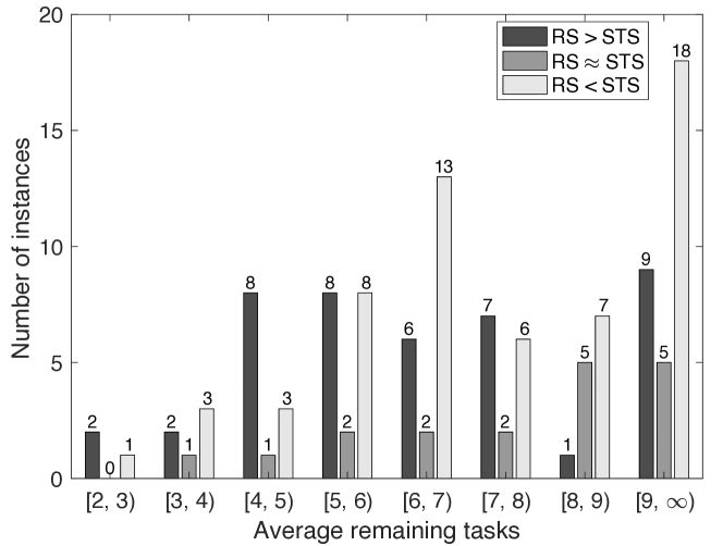
Figure 5: The number of instances for the restart strategy (RS) wins over ($\succ$), draws against ($\approx$) and loses to ($\prec$) the sequence transfer strategy (STS) for different ranges of average remaining tasks.

We also compared the rankings of each algorithm over 25 independent runs on each DCARP instance, which is presented in each cell’s bracket in Table V. The overall average rankings of each algorithm instance over 120 DCARP instances are summarised in the row of ‘Avr. Ranking’ in Table V. The Friedman test with a significance level of 0.05 was carried out to compare the ranking of eight algorithms across problem instances, leading to a p-value of 8.69e-159. This indicates that at least one pair of algorithms are not equivalent to each other. We then perform Nemenyi posthoc tests to identify which algorithms perform significantly different. The critical difference diagram is presented in Figure 6 where the value of critical difference is 0.96 [34]. We can conclude from these results that the restart and sequence transfer strategies obtained almost the same performance for population-based algorithms (MAENS and ILMA) while the sequence transfer strategy slightly outperformed the restart strategy in the individual-based algorithm (RTS) in our experiments.

Furthermore, MAENS obtains the best overall result, and RTS is the worst among the three meta-heuristic algorithms which are originally designed for static CARP. However, all of them significantly outperform the state-of-the-art dynamic algorithm, i.e. VT-MASDC and VTtr-MASDC. Recall that VT-MASDC was shown to outperform MASDC in Section V-C. Therefore, we can conclude that not only the proposed framework generalises the existing algorithms for static CARPs to solve DCARPs but also that the constructed algorithm maintains its superior performance when optimising a DCARP instance.

To evaluate the impact of parameter configuration of algorithms on our final conclusion, we have used SMAC [35] to obtain the best parameters for MAENS and MASDC, and then compared meta-heuristic algorithms with tuned parameters on additional 72 DCARP instances. The results are presented in Table VII of the supplementary material. They show clearly that MASDC with tuned parameters still performed worse than MAENS with the default or tuned parameters. MAENS with tuned parameters preformed similar to MAENS with default parameters in our experiments. In short, different parameter settings for the meta-heuristic algorithms do not change our conclusions.

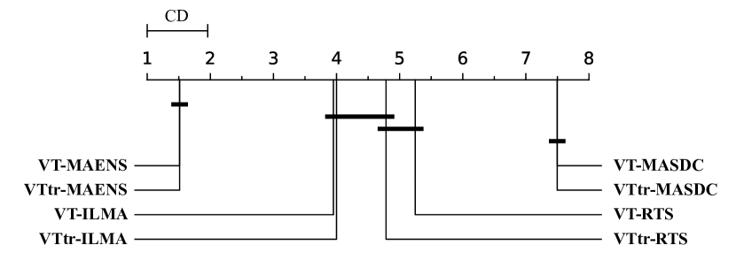
Figure 6: Critical difference diagram for the comparison of 8 algorithms against each other on egl with Friedman test and Nemenyi test. Groups of algorithms which are not significantly different at the level of 0.05 are connected.

VI Conclusion and future work

In this paper, we studied the dynamic capacitated arc routing problem (DCARP), in which dynamic events, such as road closure, added tasks, etc., occur during the vehicles’ service. First, a mathematical formulation of DCARP was provided for the first time in the literature. Then, we designed a simulation system as the research platform for DCARP. Unlike the existing benchmark generator, our simulation system generates DCARP instances from a given map in a way that is more realistic and closer to the real world. Our simulator also facilitates the use of existing algorithms for static CARP to be used for DCARP. The events simulated in our system enable existing benchmark maps from static CARP to be adopted in dynamic scenarios much closer to the real world, where dynamic events happen while a solution is being deployed, i.e., while vehicles are serving in the map. Given the mathematical model and the simulation system, we have proposed a generalised optimisation framework which can generalise algorithms for static CARPs to optimise DCARPs. In our framework, we proposed a virtual-task strategy that constructs a virtual task between the stop location and the depot, to make all outside vehicles virtually return to the depot, which tremendously simplified the optimisation for DCARP. As a result, the DCARP instance was converted into a virtual ‘static’ instance so that algorithms for static CARP can solve it.

Two initialisation strategies were adopted in our generalised optimisation framework: the restart and sequence transfer strategies. The restart strategy completely restarts the optimisation algorithm at random when there is a new DCARP instance. The sequence transfer strategy maintains the sequence of remaining tasks to the new DCARP instance and greedily inserts the new tasks into the remaining sequence, to transfer the information of task sequence from the previous optimisation experience.

In our computational study, the necessity of directly optimising DCARP together with outside vehicles was first demonstrated by comparing the virtual-task strategy with a return-first strategy. The results indicated that it would be more efficient to optimise the DCARP instance by using the virtual-task strategy when the outside vehicles’ remaining capacities were sufficiently large to serve more tasks. Then, the efficiency of the virtual-task strategy was demonstrated by embedding it into an existing algorithm and comparing it to the original version of the existing algorithm. Finally, our generalised optimisation framework’s efficiency was analysed by integrating a set of optimisation algorithms that were designed for static CARPs, and the constructed algorithms performed significantly better than state-of-the-art algorithms for DCARP.

In this paper, we have demonstrated that it is effective to solve DCARP instances by transforming them into static instances using the VT strategy and using our proposed GOFVT framework. The influence of the type and degree of dynamic events on individual optimisation algorithms was not investigated. We will further investigate the influence of different dynamic events on optimisation algorithms and design a benchmark including DCARP instances with different dynamic characteristics. Furthermore, the current sequence transfer strategy only uses the optimisation experience belonging to the instance of the previous optimisation. It would be valuable to utilise all previous search experience taken from the whole DCARP scenario. Finally, it is desirable to test our proposed framework further with large scale CARP instances and real world applications in the future.

dcarp_supplementary.pdf, 1-7

References

- [1] P. Lacomme, C. Prins, and W. Ramdane-Chérif, “Evolutionary algorithms for periodic arc routing problems,” European Journal of Operational Research, vol. 165, no. 2, pp. 535–553, 2005.
- [2] H. Handa, L. Chapman, and X. Yao, “Robust route optimization for gritting/salting trucks: A cercia experience,” IEEE Computational Intelligence Magazine, vol. 1, no. 1, pp. 6–9, 2006.
- [3] G. Ulusoy, “The fleet size and mix problem for capacitated arc routing,” European Journal of Operational Research, vol. 22, no. 3, pp. 329–337, 1985.
- [4] B. L. Golden, J. S. DeArmon, and E. K. Baker, “Computational experiments with algorithms for a class of routing problems,” Computers & Operations Research, vol. 10, no. 1, pp. 47–59, 1983.
- [5] J. Brandão and R. Eglese, “A deterministic tabu search algorithm for the capacitated arc routing problem,” Computers & Operations Research, vol. 35, no. 4, pp. 1112–1126, 2008.
- [6] K. Tang, Y. Mei, and X. Yao, “Memetic algorithm with extended neighborhood search for capacitated arc routing problems,” IEEE Transactions on Evolutionary Computation, vol. 13, no. 5, pp. 1151–1166, 2009.
- [7] K. Tang, J. Wang, X. Li, and X. Yao, “A scalable approach to capacitated arc routing problems based on hierarchical decomposition,” IEEE Transactions on Cybernetics, vol. 47, no. 11, pp. 3928–3940, 2016.
- [8] S. Wøhlk and G. Laporte, “A fast heuristic for large-scale capacitated arc routing problems,” Journal of the Operational Research Society, vol. 69, no. 12, pp. 1877–1887, Jan 2018.
- [9] M. C. Mourão and L. S. Pinto, “An updated annotated bibliography on arc routing problems,” Networks, vol. 70, no. 3, pp. 144–194, Aug 2017.
- [10] Á. Corberán, R. Eglese, G. Hasle, I. Plana, and J. M. Sanchis, “Arc routing problems: A review of the past, present, and future,” Networks, vol. 77, no. 1, pp. 88–115, 2021.
- [11] L. Xing, P. Rohlfshagen, Y. Chen, and X. Yao, “An evolutionary approach to the multidepot capacitated arc routing problem,” IEEE Transactions on Evolutionary Computation, vol. 14, no. 3, pp. 356–374, 2009.
- [12] R. K. Arakaki and F. L. Usberti, “Hybrid genetic algorithm for the open capacitated arc routing problem,” Computers & Operations Research, vol. 90, pp. 221–231, Feb 2018.
- [13] J.-M. Belenguer, E. Benavent, N. Labadi, C. Prins, and M. Reghioui, “Split-delivery capacitated arc-routing problem: Lower bound and metaheuristic,” Transportation Science, vol. 44, no. 2, pp. 206–220, May 2010.
- [14] Y. Chen and J.-K. Hao, “Two phased hybrid local search for the periodic capacitated arc routing problem,” European Journal of Operational Research, vol. 264, no. 1, pp. 55–65, Jan 2018.
- [15] J. de Armas, P. Keenan, A. A. Juan, and S. McGarraghy, “Solving large-scale time capacitated arc routing problems: from real-time heuristics to metaheuristics,” Annals of Operations Research, vol. 273, no. 1-2, pp. 135–162, Feb 2018.
- [16] M. Liu, H. K. Singh, and T. Ray, “A memetic algorithm with a new split scheme for solving dynamic capacitated arc routing problems,” in 2014 IEEE Congress on Evolutionary Computation. IEEE, 2014, pp. 595–602.
- [17] ——, “A benchmark generator for dynamic capacitated arc routing problems,” in 2014 IEEE Congress on Evolutionary Computation. IEEE, 2014, pp. 579–586.
- [18] Y. Mei, K. Tang, and X. Yao, “Evolutionary computation for dynamic capacitated arc routing problem,” in Evolutionary Computation for Dynamic Optimization Problems. Springer, 2013, pp. 377–401.
- [19] J. Liu, K. Tang, and X. Yao, “Robust optimization in uncertain capacitated arc routing problems: Progresses and perspectives,” IEEE Computational Intelligence Magazine, vol. 16, no. 1, pp. 63–82, 2021.
- [20] H. Handa, L. Chapman, and X. Yao, “Dynamic salting route optimisation using evolutionary computation,” in 2005 IEEE Congress on Evolutionary Computation, vol. 1. IEEE, 2005, pp. 158–165.
- [21] M. Tagmouti, M. Gendreau, and J.-Y. Potvin, “A dynamic capacitated arc routing problem with time-dependent service costs,” Transportation Research Part C: Emerging Technologies, vol. 19, no. 1, pp. 20–28, 2011.
- [22] M. Monroy-Licht, C. A. Amaya, A. Langevin, and L.-M. Rousseau, “The rescheduling arc routing problem,” International Transactions in Operational Research, vol. 24, no. 6, pp. 1325–1346, 2017.
- [23] W. Padungwech, J. Thompson, and R. Lewis, “Effects of update frequencies in a dynamic capacitated arc routing problem,” Networks, vol. 76, no. 4, pp. 522–538, 2020.
- [24] A. Yazici, G. Kirlik, O. Parlaktuna, and A. Sipahioglu, “A dynamic path planning approach for multi-robot sensor-based coverage considering energy constraints,” in 2009 IEEE/RSJ International Conference on Intelligent Robots and Systems. IEEE, 2009, pp. 5930–5935.
- [25] H. Tong, L. L. Minku, S. Menzel, B. Sendhoff, and X. Yao, “Towards novel meta-heuristic algorithms for dynamic capacitated arc routing problems,” in International Conference on Parallel Problem Solving from Nature. Springer, 2020, pp. 428–440.
- [26] V. Pillac, M. Gendreau, C. Guéret, and A. L. Medaglia, “A review of dynamic vehicle routing problems,” European Journal of Operational Research, vol. 225, no. 1, pp. 1–11, 2013.
- [27] L. Foulds, H. Longo, and J. Martins, “A compact transformation of arc routing problems into node routing problems,” Annals of Operations Research, vol. 226, no. 1, pp. 177–200, Sep 2014.
- [28] M. Mavrovouniotis, C. Li, and S. Yang, “A survey of swarm intelligence for dynamic optimization: Algorithms and applications,” Swarm and Evolutionary Computation, vol. 33, pp. 1–17, Apr 2017.
- [29] T. T. Nguyen, S. Yang, and J. Branke, “Evolutionary dynamic optimization: A survey of the state of the art,” Swarm and Evolutionary Computation, vol. 6, pp. 1–24, Oct 2012.
- [30] M. Mavrovouniotis and S. Yang, “Adapting the pheromone evaporation rate in dynamic routing problems,” in European Conference on the Applications of Evolutionary Computation. Springer, 2013, pp. 606–615.
- [31] L. Y. Li and R. W. Eglese, “An interactive algorithm for vehicle routeing for winter—gritting,” Journal of the Operational Research Society, vol. 47, no. 2, pp. 217–228, 1996.
- [32] Y. Mei, K. Tang, and X. Yao, “Improved memetic algorithm for capacitated arc routing problem,” in 2009 IEEE Congress on Evolutionary Computation. IEEE, 2009, pp. 1699–1706.
- [33] ——, “A global repair operator for capacitated arc routing problem,” IEEE Transactions on Systems, Man, and Cybernetics, Part B (Cybernetics), vol. 39, no. 3, pp. 723–734, 2009.
- [34] J. Demšar, “Statistical comparisons of classifiers over multiple data sets,” Journal of Machine learning research, vol. 7, no. Jan, pp. 1–30, 2006.
- [35] F. Hutter, H. H. Hoos, and K. Leyton-Brown, “Sequential model-based optimization for general algorithm configuration,” in International conference on learning and intelligent optimization. Springer, 2011, pp. 507–523.