A Dark Energy model from Generalized Proca Theory

Abstract

We consider a specific dark energy model, which only includes the Lagrangian up to the cubic order in terms of the vector field self-interactions in the generalized Proca theory. We examine the cosmological parameters in the model by using the data sets of CMB and CMB+HST, respectively. In particular, the Hubble constant is found to be $H_{0}=71.80^{+1.07}_{-0.72}$ ($72.48^{+0.72}_{-0.60}$) $\rm kms^{-1}Mpc^{-1}$ at $68\%$ C.L. with CMB (CMB+HST), which would alleviate the Hubble constant tension. We also obtain that the reduced $\chi^{2}$ values in our model are close to unity when fitting with CMB and CMB+HST, illustrating that our model is a good candidate to describe the cosmological evolutions of the universe.

I Introduction

Recent cosmological observations have shown that our universe is experiencing a late-time acceleration Riess:1998cb ; Perlmutter:1998np . The simplest attempt to explain this phenomenon is to introduce the cosmological constant $\Lambda$ as a repulsive force effectively, which is also embedded in the $\Lambda$CDM model Amendola:2015 ; Weinberg:1972 . Although the $\Lambda$CDM model is one of the most successful cosmological model describing the large-scale structure of the universe, it fails to solve the fine-tuning and coincidence problems, referred to as the cosmological constant problem Weinberg:1988cp ; Peebles:2002gy ; ArkaniHamed:2000tc .

One alternative way to account for the accelerating universe is by introducing additional degrees of freedom in the gravitational theory Copeland:2006wr . This can be achieved by either modifying the geometric part or involving some new fluids with negative pressure in the energy-momentum tensor of the Einstein field equation. In particular, a wide class of dark energy models can be constructed by adding an additional scalar field $\phi$, which contains a derivative coupling to the Ricci scalar $R$. The most general scalar-tensor theories with second-order equations of motion were derived by Horndeski in 1974 Horndeski:1974wa , which have been found to have numerous applications in cosmology, particularly in dark energy and inflation Deffayet:2011gz ; Charmousis:2011bf .

If we now replace the scalar field by a massive vector field $A^{\mu}$, the most general second-order field equations are called generalized Proca theories Heisenberg:2014rta ; Jimenez:2016isa . The application of this kind of theories to cosmology up to the sixth-order of the vector field self-interactions in the Lagrangian has been studied in both background and perturbation levels, and compared with the observational data DeFelice:2016yws ; DeFelice:2016uil ; deFelice:2017paw ; DeFelice:2020sdq ; Heisenberg:2020xak . It has been shown that there exists a de Sitter solution relevant to the late-time expansion in these theories. In addition, the authors in Ref. DeFelice:2016yws also proposed a dark energy model, in which the solution always approaches a de Sitter fixed point.

Recently, there has been the so-called Hubble tension in cosmology, indicating a mismatch between the local measurements and early-time observations for the expansion rate of the Universe, i.e. the Hubble parameter $H_{0}$. The measurements from the Hubble Space Telescope (HST) has implied the value of $H_{0}$ to be $74.03\pm 1.42$ $\rm km\;s^{-1}Mpc^{-1}$ Riess:2019cxk , whereas, the CMB measurement together with the $\Lambda CDM$ model has given $67.4\pm 0.5$ $\rm km\;s^{-1}Mpc^{-1}$ Aghanim:2018eyx . Many approaches in the literature have been presented to understand this tension, which can be divided into the early-time and late-time modifications of general relativity. Examples for the former are the early dark energy scenario Poulin:2018cxd ; Karwal:2016vyq , primodial magnetic fields Jedamzik:2020krr , dark energy-dark matter interactions Agrawal:2019dlm , while the latter includes the modified gravity theory, which is our adopted approach. In this study, we concentrate on one of the simplest dark energy model from the generalized Proca theory, in which we only consider up to the cubic order of the vector field self-interactions and present the numerical analysis of the model based on Refs. DeFelice:2020sdq .

This paper is organized as follows. In Sec. II, we present our specific model based on the generalized Proca theories along with the background equations of motion. In Sec. III, we show the global fitting results. Our conclusion is given Sec. IV. At last, we demonstrate the tensor, vector and scalar perturbations for this model in the Appendix.

II Our model with background studies

The action of the generalized Proca theory is given by Jimenez:2016isa ; Heisenberg:2014rta

$$S=\int d^{4}x\sqrt{-g}(\mathcal{L}+\mathcal{L}_{M}),$$ (1)

where $g$ is the determinant of the metric tensor $g_{\mu\nu}$, $\mathcal{L}_{M}$ is the matter Lagrangian, and $\mathcal{L}$ is given by

$$\mathcal{L}=\sum^{6}_{i=2}\mathcal{L}_{i},$$ (2)

with $\mathcal{L}_{i}$ related to the vector field self-interactions, defined by

$$\mathcal{L}_{2} =G_{2}(X,F,Y),$$

$$\mathcal{L}_{3} =G_{3}(X)\nabla_{\mu}A^{\mu},$$

$$\mathcal{L}_{4} =G_{4}(X)R+G_{4,X}(X)[(\nabla_{\mu}A^{\mu})^{2}-\nabla_{\rho}A_{\sigma}\nabla^{\sigma}A^{\rho}],$$

$$\mathcal{L}_{5} =G_{5}(X)G_{\mu\nu}\nabla^{\mu}A^{\nu}-\frac{1}{6}G_{5,X}(X)[(\nabla_{\mu}A^{\mu})^{3}-3\nabla_{\mu}A^{\mu}\nabla_{\rho}A_{\sigma}\nabla^{\sigma}A^{\rho}+2\nabla_{\rho}A_{\sigma}\nabla^{\gamma}A^{\rho}\nabla^{\sigma}A_{\gamma}]$$

$$-g_{5}(X)\tilde{F}^{\alpha\mu}\tilde{F}^{\beta}{}_{\mu}\nabla_{\alpha}A_{\beta},$$

$$\mathcal{L}_{6} =G_{6}(X)L^{\mu\nu\alpha\beta}\nabla_{\mu}A_{\nu}\nabla_{\alpha}A_{\beta}+\frac{1}{2}G_{6,X}(X)\tilde{F}^{\alpha\beta}\tilde{F}^{\mu\nu}\nabla_{\alpha}A_{\mu}\nabla_{\beta}A_{\nu},$$ (3)

where $X=-\frac{1}{2}A_{\mu}A^{\mu},F=-\frac{1}{4}F_{\mu\nu}F^{\mu\nu},Y=A^{\mu}A^{\nu}F_{\mu}{}^{\alpha}F_{\nu\alpha}$, $G_{i,X}=\partial{G_{i}}/\partial X$, $F_{\mu\nu}=\nabla_{\mu}A_{\nu}-\nabla_{\nu}A_{\mu},\tilde{F}^{\mu\nu}=\frac{1}{2}\epsilon^{\mu\nu\alpha\beta}F_{\alpha\beta},andL^{\mu\nu\alpha\beta}=\frac{1}{4}\epsilon^{\mu\nu\rho\sigma}\epsilon^{\alpha\beta\gamma\delta}R_{\rho\sigma\gamma\delta}$, with $\nabla_{\mu}$, $\epsilon^{\mu\nu\alpha\beta}$, and $R_{\rho\sigma\gamma\delta}$ corresponding to the covariant derivative operator, Levi-Civita tensor and Riemann tensor, respectively.

II.1 Background Equations of Motion

For the homogeneity and isotropy of the universe, we consider the metric to be the flat Friedmann-Lemaitre-Robertson-Walker (FLRW) one, given by

$$ds^{2}=-dt^{2}+a^{2}(t)\delta_{ij}dx^{i}dx^{j},$$ (4)

with $a(t)$ the scale factor, and the Proca vector field $A^{\mu}$

$$A^{\mu}=(\phi(t),0,0,0).$$ (5)

In Eq. (2), we only concentrate on the terms up to the cubic order with $G_{4}(X)=G_{4}$ being a constant. As a result, the background equations of motion can be obtained by varying the action (1) DeFelice:2016yws ; DeFelice:2016uil ; deFelice:2017paw ; DeFelice:2020sdq , given by

$$G_{2}-G_{2.X}\phi^{2}-3G_{3,X}H\phi^{3}+6G_{4}H^{2}=\rho_{M},$$ (6)

$$G_{2}-\dot{\phi}\phi^{2}G_{3,X}+2G_{4}(3H^{2}+2\dot{H})=-P_{M},$$ (7)

$$\phi(G_{2,X}+3G_{3,X}H\phi)=0.$$ (8)

where $G_{i,X}=\partial G_{i}/\partial X$, and the dot denotes the derivative with respect to cosmic time $t$. Here, we note that the perfect fluid has been taken into account. That is, the energy-momentum tensor for matter can be written as $T^{\mu}{}_{\nu}=\text{diag}(-\rho_{M},P_{M},P_{M},P_{M})$ with $\rho_{M}$ ($P_{M}$) representing the energy density (pressure). The matter sector is assumed to be composed of non-relativistic matter ($m$) and radiation ($r$) with continuity equations read as:

$$\dot{\rho}_{m,r}+3H(1+w_{m,r})\rho_{m,r}=0,$$ (9)

where and the equations of state are defined by

$$w_{m,r}=\frac{P_{m,r}}{\rho_{m,r}}=0,\frac{1}{3}.$$ (10)

The energy density and pressure then become $\rho_{M}=\rho_{m}+\rho_{r}$ and $P_{M}=\rho_{r}/3$, respectively.

For dark energy to be dominated in the late-time cosmological epoch, the amplitude of the temporal component of the vector field $\phi$ should increase as the Hubble parameter decreases. As suggested in Refs. DeFelice:2016yws ; DeFelice:2016uil ; deFelice:2017paw , we can use the relation, given by

$$\phi^{p}\propto H^{-1},$$ (11)

where $p$ is a positive constant. Consequently, the functions of $G_{2,3}$ can be chosen to be the powers of $X$:

$$G_{2}(X,F)=F+b_{2}X^{p_{2}},\quad G_{3}(X)=b_{3}X^{p_{3}}.$$ (12)

Besides, we let $G_{4}(X)=M_{pl}^{2}/2$, where $M_{pl}$ is the reduced Planck mass, in accordance with general relativity. In order to satisfy (8), there are some constraints on the parameters of $b$ and $p$, given by

$$p_{3}=\frac{1}{2}(p+2p_{2}-1),$$ (13)

$$2^{p_{3}-p_{2}}p_{2}b_{2}+3p_{3}b_{3}(\phi^{p}H)=0.$$ (14)

In our calculation, we introduce a new free parameter $s$, defined by

$$s\equiv\frac{p_{2}}{p}\,,$$ (15)

which is relevant to the background evolution and has been already fitted in the literature. In particular, in Ref. deFelice:2017paw it is found that $s=0.254^{+0.118}_{-0.097}$ with the CMB data by Planck, while it shifted to $s=0.16\pm{0.08}$ when the RSD data is included. For simplicity and illustrating our results, we fix the parameter of $s$ to be 0.25 by hand, and then choose a simple set:

$$p_{2} =1,\quad p=4;\quad s=0.25\,.$$ (16)

Consequently, the resulting modified Friedmann equations become

$$3M_{pl}^{2}H^{2} =\rho_{M}+\rho_{DE},$$ (17)

$$M_{pl}^{2}(3H^{2}+2\dot{H}) =-P_{M}-P_{DE},$$ (18)

where $\rho_{DE}$ ($P_{DE}$) is the energy density (pressure) of dark energy, given by

$$\rho_{DE} =-\frac{1}{2}b_{2}\phi^{2},$$ (19)

$$P_{DE} =\frac{1}{2}b_{2}\phi^{2}+\frac{1}{3}b_{2}\dot{\phi}\phi H^{-1}.$$ (20)

Note that $b_{2}$ and $b_{3}$ are related by

$$b_{3} =-\frac{4\sqrt{2}}{15(\phi^{4}H)}b_{2}$$ (21)

based on (14).

II.2 Background Cosmological Evolutions

To study the cosmological evolutions, it is convenient to introduce the density parameters, defined as

$$\Omega_{i}=\frac{\rho_{i}}{3M_{pl}^{2}H^{2}},$$ (22)

where $i=m,r,DE$, and

$$\Omega_{m}+\Omega_{r}+\Omega_{DE}=1.$$ (23)

Taking derivatives of $\eqref{om}$ and using of (7) and (8), the equations of motion for the energy densities can be written as DeFelice:2016yws :

$$\Omega^{\prime}_{DE} =\frac{(1+s)\Omega_{DE}(3+\Omega_{r}-3\Omega_{DE})}{1+s\Omega_{DE}},$$ (24)

$$\Omega^{\prime}_{r} =-\frac{\Omega_{r}[1-\Omega_{r}+(3+4s)\Omega_{DE}]}{1+s\Omega_{DE}},$$ (25)

where a prime denotes the derivative respect to the e-folding number $N\equiv\ln a$. Using Eqs. (22)-(25) and initial conditions of the density parameters, the evolutions of $\Omega_{m,r,DE}$ in (22) can be solved. The equation of state for dark energy, which is defined by (19) and (20), can also be written as:

$$w_{DE}\equiv\frac{P_{DE}}{\rho_{DE}}={-\frac{3(1+s)+s\Omega_{r}}{3(1+s\Omega_{DE})}}.$$ (26)

Using Eq. (16) in our model, Eqs. (24)-(26) become

$$\Omega^{\prime}_{DE} =\frac{5\Omega_{DE}(3+\Omega_{r}-3\Omega_{DE})}{4+\Omega_{DE}},$$ (27)

$$\Omega^{\prime}_{r} =-\frac{4\Omega_{r}(1-\Omega_{r}+4\Omega_{DE})}{4+\Omega_{DE}},$$ (28)

$$w_{DE} =-\frac{15+\Omega_{r}}{3(4+\Omega_{DE})},$$ (29)

respectively. The evolutions of $w_{DE}$ and the density parameter versus the redshift $z$ for our specific model are plotted in Figs. 1 and 2, respectively. It can be seen that $w_{DE}$ evolves from $w_{DE}=-1-(4/3)s\approx-1.33$ in radiation era when $(\Omega_{r},\Omega_{DE})=(1,0)$ to $w_{DE}=-1-s=-1.25$ in matter era when $(\Omega_{r},\Omega_{DE})=(0,0)$, and $w_{DE}=-1.06$ at present, which shows an phantom-like behavior with $w_{DE}<-1$  Heisenberg:2020xak .

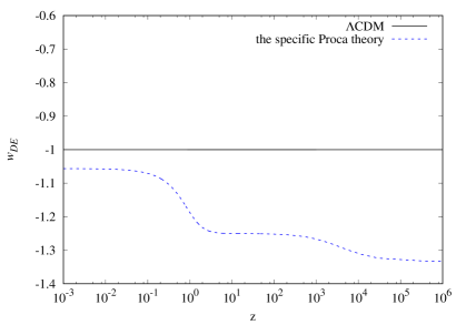
Figure 1: Evolutions of equation of state for dark energy, $w_{DE}$, versus redshift for the model and $\Lambda$CDM

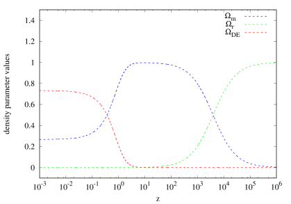
Figure 2: Evolutions of density parameters for matter ($\Omega_{m}$), radiation ($\Omega_{r}$) and dark energy ($\Omega_{DE}$) versus redshift for our model. The initial value are give by ($\Omega_{m}^{0}$, $\Omega_{r}^{0}$, $\Omega_{DE}^{0}$) = $(0.266,6.83\times 10^{-5},0.733)$, where “0” denotes for the value at present.

III Global Fitting Results

We use the CosmoMC Lewis:2002ah and CAMB Lewis:1999bs packages to study the constraints on cosmological parameters at the background level of our specific model in this section. The CosmoMC package is a MCMC engine, which can be used to explore the parameter space based on maximum likelihood method.

To examine the behaviors of our model on the evolutions of the universe, we fit the models with the combination of the CMB and Hubble constant data sets. The CMB data include temperature and polarization angular power spectra from Planck 2018 with TT, TE, EE, low-$l$ polarization, and CMB lensing from SMICA Aghanim:2018eyx ; Aghanim:2018oex ; Akrami:2019izv ; Aghanim:2019ame , while the Hubble constant of $H_{0}=74.03\pm 1.42$ $\rm km\;s^{-1}Mpc^{-1}$ is from Hubble Space Telescope (HST)  Riess:2019cxk . As we set $s=0.25$ and let the neutrino mass sum be a free parameter, both our model and $\Lambda$CDM contain seven free parameters, where the priors are listed in Table 1. To obtain the best fitted values of cosmological parameters, we use the $\chi^{2}$ method with

$$\chi^{2}={\chi^{2}_{CMB}+\chi^{2}_{HST}}\,,$$ (30)

Explicitly, we take

$$\chi^{2}_{CMB}=(x^{th}_{i,CMB}-x^{obs}_{i,CMB})(C^{-1}_{CMB})_{ij}(x^{th}_{j,CMB}-x^{obs}_{j,CMB})\,,$$ (31)

where “th” and “obs” denote theory and observational values, respectively, $C^{-1}_{CMB}$ is the inverse covariance matrix, and $x_{i,CMB}\equiv(l_{A}(z_{*}),R(z_{*}),z_{*})$ with the acoustic scale $l_{A}$ and the shift parameter $R$ at the photon decoupling epoch, $z_{*}$, defined by

$$l_{A}(z_{*}) = (1+z_{*})\frac{\pi D_{A}(z_{*})}{r_{s}(z_{*})}\,,$$

$$R(z_{*}) \equiv (1+z_{*})D_{A}(z_{*})\sqrt{\Omega_{m}H^{2}_{0}}\,.$$ (32)

In Eq. (32), $D_{A}(z)$ and $r_{s}$ are the proper angular diameter distance and comoving sound horizon, given by

$$D_{A}(z) = \frac{1}{1+z}\int_{0}^{z}\frac{dz^{{}^{\prime}}}{H(z^{{}^{\prime}})}\,,$$

$$r_{s}(z) = \frac{1}{\sqrt{3}}\int_{0}^{1/(1+z)}\frac{da}{a^{2}H(a)\sqrt{1+(3\Omega^{0}_{b}/4\Omega^{0}_{r})a}}\,,$$ (33)

respectively, where $\Omega^{0}_{b}$ and $\Omega^{0}_{r}$ present values of baryon and photon density parameters, respectively. For $\chi^{2}_{HST}$ , we have

$$\chi^{2}_{HST}=\frac{(74.03-H^{th}_{0})^{2}}{1.42^{2}}\,,$$ (34)

where $H^{th}_{0}$ is the theoretical value of Hubble parameter in the model.

To compare the results between the models, we use the reduced $\chi^{2}$, defined by

$$\chi^{2}_{reduced}=\frac{\chi^{2}}{\nu}\,,$$ (35)

where $\nu=N-n$ is the degrees of freedom, with “N” and “n” denote as the numbers of data points and free parameters, respectively.

Table 1: Priors of the cosmological parameters for our model and $\Lambda$CDM

Parameter	Prior
Baryon density	$0.5\leq 100\Omega_{b}^{0}h^{2}\leq 10$
CDM density	$0.1\leq 100\Omega_{c}^{0}h^{2}\leq 99$
Optical depth	$0.01\leq\tau\leq 0.8$
Neutrino mass sum	$0\leq\Sigma m_{\nu}\leq 2$ eV
$\frac{\mathrm{Sound\ horizon}}{\mathrm{Angular\ diameter\ distance}}$	$0.5\leq 100\theta_{MC}\leq 10$
Scalar power spectrum amplitude	$2\leq\ln\left(10^{10}A_{s}\right)\leq 4$
Spectral index	$0.8\leq n_{s}\leq 1.2$

The constraints for the cosmological parameters of our model from the specific Proca theory with CMB and CMB+HST are plotted in Fig. 3 and listed in Table 2. It is given that $H_{0}=71.80^{+1.07}_{-0.72}$ ($72.48^{+0.72}_{-0.60}$) $\rm km\;s^{-1}Mpc^{-1}$ in our model and $H_{0}=66.75^{+1.52}_{-0.73}$ ($69.13\pm 0.57$) $\rm km\;s^{-1}Mpc^{-1}$ in $\Lambda$CDM when fitting with CMB (CMB+HST) at $68\%$ C.L. It is interesting to see that our model favors a larger $H_{0}$ even without including the HST data, while the addition of HST pulls $H_{0}$ to an even larger value, agreeing better with the local measurements.

While the early-time observation from Planck provides $H_{0}=67.4\pm 0.5$ $\rm km\;s^{-1}Mpc^{-1}$ with the $\Lambda$CDM scenario Aghanim:2018eyx , late-time measurements of $H_{0}$ exceed early-time estimation to the extent more than $4\sigma$ Riess:2020sih . This Hubble constant tension may call for new physics beyond $\Lambda$CDM with different behavior in early and late times of the universe Riess:2019cxk ; Odintsov:2020qzd . On the other hand, the generalized Proca theory, which has phantom-like behavior of $w_{DE}$ with $s>0$, naturally favors a larger $H_{0}$ and is helpful to resolve the $H_{0}$ tension deFelice:2017paw ; DeFelice:2020sdq ; Heisenberg:2020xak .

With the specific choice of the Lagrangian in the model, our result of $H_{0}=71.80^{+1.07}_{-0.72}$ ($72.48^{+0.72}_{-0.60}$) with CMB (CMB+HST) matches the late-universe measurements of $74.03\pm 1.42$ from HST Riess:2019cxk , $73.5\pm 1.4$ from SH0ES Reid:2019tiq , $75.3^{+3.0}_{-2.9}$ from H0LiCOW Wei:2020suh and $73.9\pm 3.0$ from Megamaser Pesce:2020xfe , in units of $\rm km\;s^{-1}Mpc^{-1}$ for $H_{0}$. This is caused by the phantom-like behavior in our model as plotted in Fig. 1. Moreover, the $H_{0}$ tension is reduced from $3.68\sigma$ ($3.20\sigma$) in $\Lambda$CDM to $1.30\sigma$ ($0.99\sigma$) in our model with CMB (CMB+HST).

In addition, we obtain the best fits with $\chi^{2}_{Proca,reduced}=1.0960$ ($1.0959$) and $\chi^{2}_{\Lambda CDM,reduced}=1.0964$ ($1.1016$) when fitting with CMB (CMB+HST), resulting in that $|\chi^{2}_{Proca,reduced}-1|=0.0960$ ($0.0959$) and $|\chi^{2}_{LCDM,reduced}-1|=0.0964$ ($0.1016$). As $\chi^{2}_{Proca,reduced}$ is closer to unity, our model can well describe the late-time evolution of the universe.

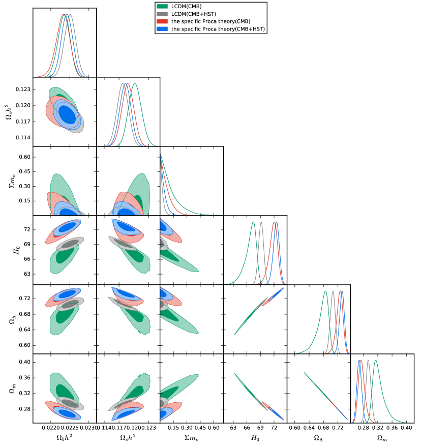
Figure 3: One and two-dimensional distributions of $\Omega_{b}^{0}h^{2}$, $\Omega_{c}^{0}h^{2}$, $\sum m_{\nu}$, $H_{0}$, $\Omega_{\Lambda}^{0}$, $\Omega_{m}^{0}$ for our model and $\Lambda$CDM with the combined data of CMB and CMB + HST, where the contour lines represent 68$\%$  and 95$\%$  C.L., respectively.

Table 2: Fitting results in our model and $\Lambda$CDM with the CMB and CMB + HST data sets, where the cosmological parameters are constrained at 68$\%$ C.L and the $H_{0}$ tension is compared with $H_{0}=74.03\pm 1.42$ $\rm km\;s^{-1}Mpc^{-1}$ from HST, by assuming the Gaussian distribution for 1D posterior.

Parameter	CMB		CMB+HST
Model	our model	$\Lambda$CDM	our model	$\Lambda$CDM
$100\Omega_{b}^{0}h^{2}$	$2.232^{+0.019}_{-0.017}$	$2.234^{+0.017}_{-0.014}$	$2.242\pm 0.015$	$2.251\pm 0.015$
$100\Omega_{c}^{0}h^{2}$	$11.88\pm 0.12$	$12.03^{+0.12}_{-0.14}$	$11.83\pm 0.11$	$11.78\pm 0.12$
$H_{0}$ ($\rm kms^{-1}Mpc^{-1}$)	$71.80^{+1.07}_{-0.72}$	$66.75^{+1.52}_{-0.73}$	$72.48^{+0.72}_{-0.60}$	$69.13\pm 0.57$
$\Omega_{DE}^{0}$	$0.7329^{+0.0103}_{-0.0073}$	$0.6766^{+0.0201}_{-0.0089}$	$0.7313^{+0.0071}_{-0.0062}$	$0.7059^{+0.0068}_{-0.0070}$
$\Omega_{m}^{0}$	$0.2754^{+0.0073}_{-0.0103}$	$0.3234^{+0.0089}_{-0.0200}$	$0.2687^{+0.0062}_{-0.0071}$	$0.2941^{+0.0070}_{-0.0068}$
$H_{0}$ tension	1.30$\sigma$	3.68$\sigma$	0.99$\sigma$	3.20$\sigma$
Reduced $\chi^{2}_{best-fit}$	$1.0960$	$1.0964$	$1.0959$	$1.1016$

Using the fitting results, we plot the evolutions of the Hubble parameter in our model and $\Lambda$CDM in Fig. 4 with the initial conditions given by best-fit values listed in Table 2. The residue of $H(z)_{Proca}-H(z)_{\Lambda CDM}$ are plotted in Fig. 5. We note that $H(z)_{Proca}>H(z)_{\Lambda CDM}$ at the low redshift region when $z\lesssim 0.55$. However, $H(z)_{\Lambda CDM}$ will surpass $H(z)_{Proca}$ at the higher redshift one when $z>0.55$.

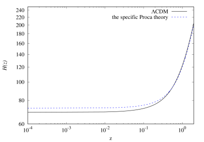
Figure 4: Evolution of Hubble parameter, $H(z)$, in the model and $\Lambda$CDM using the best-fit values from CMB+HST as initial conditions.

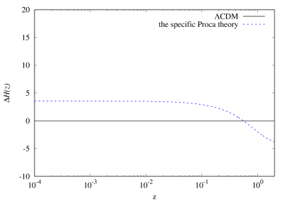
Figure 5: Evolution of Residues of Hubble parameter for the model and $\Lambda$CDM.

IV Conclusion

We have studied a specific dark energy model based on the generalized Proca theories by only including up to the cubic order in the Lagrangian. We have noticed that the dark energy evolution does not depend on the values of $b_{2}$ and $b_{3}$ but $s$. We have shown the phantom-like behavior of $w_{DE}$ and evolutions of $\Omega_{m,r,DE}$ in the model. By using the CosmoMC and CAMB packages and fitting with the observational data of the CMB data form Planck 2018 and the Hubble constant of $H_{0}=74.03\pm 1.42$ $\rm km\;s^{-1}Mpc^{-1}$ from HST, we have constrained the cosmological parameters. In particular, we have obtained that $|\chi^{2}_{Proca,reduced}-1|=0.0960$ ($0.0959$) and $|\chi^{2}_{LCDM,reduced}-1|=0.0964$ ($0.1016$) when fitting with CMB (CMB+HST).

As the generalized Proca theory is able to alleviate the $H_{0}$ tension at the background level deFelice:2017paw , our specific choice of the cubic order in terms of the vector field self-interactions in the Lagrangian also prefers a larger value of $H_{0}$, determined to be $H_{0}^{Proca}=71.80^{+1.07}_{-0.72}$ ($72.48^{+0.72}_{-0.60}$) $\rm km\;s^{-1}Mpc^{-1}$ and $H_{0}^{\Lambda CDM}=66.75^{+1.52}_{-0.73}$ ($69.13\pm 0.57$) $\rm km\;s^{-1}Mpc^{-1}$ at $68\%$ C.L. with CMB (CMB+HST). The increased value of $H_{0}$ in our model matches the local measurements of HST, SH0ES, H0LiCOW and Megamaser, resulting in that the $H_{0}$ tension is reduced to $\sim 1\sigma$ by comparing with the HST data. Furthermore, we have plotted the evolution of $H(z)$ with the initial conditions given by the best-fit from the global fitting results, and found that $H(z)_{Proca}>H(z)_{\Lambda CDM}$ at the low redshift with $z\lesssim 0.55$.

V Appendix: Perturbations

In this Appendix, we briefly list all the perturbed quantities in tensor, vector, and scalar perturbations and outline the perturbation equations for our specific dark energy model from the Generalized Proca theory, as in Refs. DeFelice:2016yws ; DeFelice:2016uil ; deFelice:2017paw . We also adopt the method described in Ref. DeFelice:2016yws . Specifically, we first expand  (1) up to the second order in perturbations, and then vary the second-order action with respect to the perturbed quantities to arrive at the perturbation equations. To perturb the gravity part of the action, we take the perturbing line element Kodama:1985bj ; Mukhanov:1990me ,

$$ds^{2}=-(1+2\alpha)dt^{2}+2(\partial_{i}\chi+V_{i})dtdx^{i}+a^{2}(t)(\delta_{ij}+h_{ij})dx^{i}dx^{j},$$ (36)

and the Proca vector field $A^{\mu}$,

$$A^{0} =\phi(t)+\delta\phi,$$ (37)

$$A^{i} =\frac{1}{a^{2}(t)}\delta^{ij}(\partial_{j}\chi_{V}+E_{j}),$$ (38)

where ($\alpha,\chi$) and ($\delta\phi,\chi_{V}$) are the scalar perturbations of the metric and $A^{\mu}$, respectively, while $V_{i}$, $h_{ij}$, and $E_{i}$ satisfy the conditions:

$$\partial^{i}V_{i} =0,$$ (39)

$$\partial^{i}h_{ij} =0,\quad h^{i}{}_{i}=0,$$ (40)

$$\partial^{i}E_{i} =0.$$ (41)

In addition, we consider the perturbations of the matter action by using the Schutz-Sorkin action Schutz:1977df ; Brown:1992kc ,

$$S_{M}=-\int d^{4}x[\sqrt{-g}\rho_{M}(n)+J^{\mu}(\partial_{\mu}l+\mathcal{A}_{1}\partial_{\mu}\mathcal{B}_{1}+\mathcal{A}_{2}\partial_{\mu}\mathcal{B}_{2})]$$ (42)

where $\rho_{M}$ depends on the number density of the fluid $n$ defined by

$$n=\sqrt{\frac{g_{\alpha\beta}J^{\alpha}J^{\beta}}{g}}.$$ (43)

We note that in this action, the pressure $P_{M}$ is related to $\rho_{M}$ by Schutz:1977df ; Brown:1992kc

$$P_{M}=n_{0}\rho_{M,n}-\rho_{M}$$ (44)

with $n_{0}$ the number density of the fluid in the background. Besides, $l$ is a scalar, whereas $J^{\mu}$ is the vector field of weight one, $\mathcal{A}_{1,2}$ and $\mathcal{B}_{1,2}$ are scalars whose perturbations are meant to describe the vector modes. For the FLRW background, $J^{0}$ corresponds to the total fluid number $\mathcal{N}_{0}$. They can be expressed as DeFelice:2016uil

$$l =-\int^{t}\rho_{M,n}dt^{\prime}-\rho_{M,n}v,$$ (45)

$$J^{0} =\mathcal{N}_{0}+\delta J,$$ (46)

$$J^{i} =\frac{1}{a^{2}}\delta^{ik}(\partial_{k}\delta j+W_{k}),$$ (47)

where $W_{k}$ also obeys the transverse condition,

$$\partial^{k}W_{k}=0.$$ (48)

For the quantities of $\mathcal{A}_{1,2}$ and $\mathcal{B}_{1,2}$, we choose the simplest forms satisfying the required properties for the vector mode as in Ref. DeFelice:2016uil , given by

$$\mathcal{A}_{1}=\delta\mathcal{A}_{1}(t,z),\quad\mathcal{A}_{2}=\delta\mathcal{A}_{2}(t,z),\quad\mathcal{B}_{1}=x+\delta\mathcal{B}_{1},\quad\mathcal{B}_{2}=y+\delta\mathcal{B}_{2}(t,z),$$ (49)

where $\delta\mathcal{A}_{i}$ and $\delta\mathcal{B}_{i}$ are perturbed quantities.

V.1 Tensor perturbations

For the tensor perturbation $h_{ij}$ to the metric, we use the transverse and traceless conditions (40). To be specific, we express the components of $h_{ij}$ to be $h_{ij}=h_{+}e_{ij}^{+}+h_{\times}e_{ij}^{\times}$, where $e_{ij}^{+}$ and $e_{ij}^{\times}$ obey the relations of $e_{ij}^{+}(\bm{k})e_{ij}^{+}(\bm{-k})^{\ast}=1$, $e_{ij}^{\times}(\bm{k})e_{ij}^{\times}(\bm{-k})^{\ast}=1$, and $e_{ij}^{+}(\bm{k})e_{ij}^{\times}(\bm{-k})^{\ast}=0$ in the Fourier space with $\bm{k}$ being the comoving wave number. To obtain the tensor perturbation equations for our model, we first expand the action (1) up to the second order  DeFelice:2016yws ; DeFelice:2016uil ; deFelice:2017paw ,

$$S^{(2)}_{T}=\sum_{\lambda=+,\times}\int dt\,d^{3}x\,M_{pl}^{2}\frac{a^{3}}{8}\Big{[}\dot{h}_{\lambda}^{2}-\frac{1}{a^{2}}(\partial h_{\lambda}^{2})\Big{]}.$$ (50)

Vary the above action (50), we find that

$$\ddot{h}_{\lambda}+3H\dot{h}_{\lambda}+\frac{k^{2}}{a^{2}}h_{\lambda}=0,$$ (51)

where $k=\left|\bm{k}\right|$. We note that this is identical to the one in general relativity.

V.2 Vector perturbations

For the vector perturbations, the dynamical field $\tilde{Z}_{i}$ can be expressed in terms of the combination of $E_{i}$ and $V_{i}$, given by

$$\tilde{Z}_{i}=\frac{1}{a}[E_{i}+\phi(t)V_{i}]\,.$$ (52)

Due to the transverse condition, $\partial^{i}\tilde{Z}_{i}=0$, we can choose that $\tilde{Z}_{i}=(\tilde{Z}_{1}(t,z),\tilde{Z}_{2}(t,z),0)$ without loss of generality. Similar to the case in the tensor perturbations, by expanding the action (1) up to the second order, taking the small-scale limit, and plugging in Eqs. (12) and (16), the resulting action becomes DeFelice:2016uil

$$S^{(2)}_{V}\approx\int dt\,d^{3}x\,\sum_{i=1}^{2}\frac{a^{3}}{2}\Big{[}\dot{\tilde{Z}}_{i}^{2}+\frac{k^{2}}{a^{2}}\tilde{Z}_{i}^{2}\Big{]},$$ (53)

which is similar to (50). As a result, the equations of motion for the vector perturbations are also similar to those in the tensor perturbations,

$$\ddot{\tilde{Z}}_{i}+3H\dot{\tilde{Z}}_{i}+\frac{k^{2}}{a^{2}}\tilde{Z}_{i}=0.$$ (54)

V.3 Scalar perturbations

For the scalar perturbations, the dynamical fields are $\psi=\chi_{V}+\phi(t)\chi$ and $\delta\rho_{M}$. Expanding the action (1) up to the second order in our choices of the parameters, one gets that DeFelice:2016uil

$$S^{(2)}_{S} =\int dtd^{3}x\,a^{3}\bigg{\{}-\frac{n_{0}\rho_{M,n}}{2a^{2}}(\partial v)^{2}+\bigg{[}n_{0}\rho_{M,n}\frac{\partial^{2}\chi}{a^{2}}-\dot{\delta}\rho_{M}-3H(1+c_{M}^{2})\delta\rho_{M}\bigg{]}v$$

$$- \frac{c_{M}^{2}}{2n_{0}\rho_{M,n}}(\delta\rho_{M})^{2}-\alpha\delta\rho_{M}+2\frac{\phi^{2}}{a^{2}}(\partial\alpha)^{2}-(3M_{pl}^{2}H^{2}+b_{2}\phi^{2})\alpha^{2}$$

$$- \bigg{[}3b_{2}\phi\delta\phi+\frac{2\phi}{a^{2}}\partial^{2}(\delta\phi)+\frac{2\phi}{a^{2}}\partial^{2}\dot{\psi}+\frac{b_{2}\phi}{3a^{2}H}\partial^{2}\psi\bigg{]}\alpha$$

$$- \frac{(\partial\delta\phi)^{2}}{2a^{2}}-2b_{2}(\delta\phi)^{2}-\bigg{[}\frac{b_{2}}{3H}\psi+\dot{\psi}\bigg{]}\frac{\partial^{2}(\delta\phi)}{a^{2}}$$

$$- \frac{(\partial\dot{\psi})^{2}}{2a^{2}}+\frac{b_{2}\dot{\phi}}{6\phi Ha^{2}}(\partial\psi)^{2}+\bigg{[}(-2M_{pl}^{2}H+\frac{b_{2}\phi^{2}}{3H})\alpha+\frac{b_{2}\phi}{3H}\delta\phi\bigg{]}\frac{\partial^{2}\chi}{a^{2}}\bigg{\}}\,,$$ (55)

where $c_{M}$ corresponds to the matter propagation speed, given by DeFelice:2016uil

$$c_{M}^{2}=\frac{n_{0}\rho_{M,nn}}{\rho_{M,n}},$$ (56)

and the matter perturbation $\delta\rho_{M}$ is defined by

$$\delta\rho_{M}=\frac{\rho_{M,n}}{a^{3}}\delta J=\frac{\rho_{M}+P_{M}}{n_{0}a^{3}}\delta J.$$ (57)

Vary the action (V.3), the equations of motion in the Fourier space for $\alpha,\chi,\delta\phi,v,\delta\psi$, and $\delta\rho_{M}$ are given by

$$\delta\rho_{M}+(6M_{pl}^{2}H^{2}+2b_{2}\phi^{2})\alpha+3b_{2}\phi\delta\phi+\frac{k^{2}}{a^{2}}\bigg{[}\mathcal{Y}-2M_{pl}^{2}H\chi+\frac{b_{2}\phi}{3H}(\phi\chi-\psi)\bigg{]}=0,$$ (58)

$$(\rho_{M}+P_{M})v+\bigg{(}\frac{b_{2}\phi^{2}}{3H}-2M_{pl}^{2}H\bigg{)}\alpha+\frac{b_{2}\phi}{3H}\delta\phi=0,$$ (59)

$$3b_{2}\phi^{2}+4b_{2}\phi\delta\phi+\frac{k^{2}}{a^{2}}\bigg{[}\frac{1}{2}\mathcal{Y}+\frac{b_{2}\phi}{3H}(\phi\chi-\psi)\bigg{]}=0,$$ (60)

$$\dot{\delta}\rho_{M}+3H(1+c_{M}^{2})\delta\rho_{M}+\frac{k^{2}}{a^{2}}(\rho_{M}+P_{M})(\chi+v)=0,$$ (61)

$$\dot{\mathcal{Y}}+\bigg{(}H-\frac{\dot{\phi}}{\phi}\bigg{)}\mathcal{Y}+\frac{2b_{2}}{3H}(\phi^{2}\alpha+\dot{\phi}\psi)+\frac{2b_{2}\phi}{3H}\delta\phi=0,$$ (62)

$$\dot{v}-3Hc_{M}^{2}v-c_{M}^{2}\frac{\delta\rho_{M}}{\rho_{M}+P_{M}}-\alpha=0,$$ (63)

respectively, where

$$\mathcal{Y}\equiv-2\phi\dot{\psi}-2\phi\delta\phi-4\alpha\phi^{2}.$$ (64)

References

- (1) A. G. Riess et al. [Supernova Search Team], Astron. J. 116, 1009 (1998).
- (2) S. Perlmutter et al. [Supernova Cosmology Project], Astrophys. J. 517, 565 (1999).
- (3) L. Amendola and S. Tsujikawa, Dark Energy : Theory and Observations, (Cambridge Univer- sity Press, 2015).
- (4) S. Weinberg, Gravitation and Cosmology, (Wiley and Sons, New York, 1972).
- (5) S. Weinberg, Rev. Mod. Phys. 61, 1 (1989).
- (6) P. J. E. Peebles and B. Ratra, Rev. Mod. Phys. 75, 559 (2003).
- (7) N. Arkani-Hamed, L. J. Hall, C. F. Kolda and H. Murayama, Phys. Rev. Lett. 85, 4434 (2000).
- (8) E. J. Copeland, M. Sami and S. Tsujikawa, Int. J. Mod. Phys. D 15, 1753 (2006).
- (9) G. W. Horndeski, Int. J. Theor. Phys. 10, 363 (1974).
- (10) C. Deffayet, X. Gao, D. Steer and G. Zahariade, Phys. Rev. D 84, 064039 (2011).
- (11) C. Charmousis, E. J. Copeland, A. Padilla and P. M. Saffin, Phys. Rev. Lett. 108, 051101 (2012).
- (12) L. Heisenberg, JCAP 05, 015 (2014).
- (13) J. Beltran Jimenez and L. Heisenberg, Phys. Lett. B 757, 405 (2016).
- (14) A. De Felice, L. Heisenberg, R. Kase, S. Mukohyama, S. Tsujikawa and Y. Zhang, JCAP 06, 048 (2016).
- (15) A. De Felice, L. Heisenberg, R. Kase, S. Mukohyama, S. Tsujikawa and Y. Zhang, Phys. Rev. D 94, 044024 (2016).
- (16) A. de Felice, L. Heisenberg and S. Tsujikawa, Phys. Rev. D 95, 123540 (2017).
- (17) A. De Felice, C. Q. Geng, M. C. Pookkillath and L. Yin, JCAP 2008, 038 (2020).
- (18) L. Heisenberg and H. Villarrubia-Rojo, arXiv:2010.00513 [astro-ph.CO].
- (19) A. G. Riess, S. Casertano, W. Yuan, L. M. Macri and D. Scolnic, Astrophys. J. 876, 85 (2019).
- (20) N. Aghanim et al. [Planck], arXiv:1807.06209 [astro-ph.CO].
- (21) V. Poulin, T. L. Smith, T. Karwal and M. Kamionkowski, Phys. Rev. Lett. 122, 221301 (2019).
- (22) T. Karwal and M. Kamionkowski, Phys. Rev. D 94, 103523 (2016).
- (23) K. Jedamzik and L. Pogosian, Phys. Rev. Lett. 125, 181302 (2020).
- (24) P. Agrawal, G. Obied and C. Vafa, arXiv:1906.08261 [astro-ph.CO].
- (25) S. Nakamura, A. De Felice, R. Kase and S. Tsujikawa, Phys. Rev. D 99, 063533 (2019).
- (26) A. Lewis and S. Bridle, Phys. Rev. D 66, 103511 (2002).
- (27) A. Lewis, A. Challinor and A. Lasenby, Astrophys. J. 538, 473 (2000).
- (28) N. Aghanim et al. [Planck Collaboration], arXiv:1807.06210 [astro-ph.CO].
- (29) Y. Akrami et al. [Planck Collaboration], arXiv:1905.05697 [astro-ph.CO].
- (30) N. Aghanim et al. [Planck], arXiv:1907.12875 [astro-ph.CO].
- (31) A. G. Riess, Nature Rev. Phys. 2, 10 (2019)
- (32) S. D. Odintsov, D. S. C. Gómez and G. S. Sharov, arXiv:2011.03957 [gr-qc].
- (33) M. J. Reid, D. W. Pesce and A. G. Riess, Astrophys. J. Lett. 886, L27 (2019).
- (34) J. J. Wei and F. Melia, Astrophys. J. 897, 127 (2020)
- (35) D. W. Pesce, J. A. Braatz, M. J. Reid, A. G. Riess, D. Scolnic, J. J. Condon, F. Gao, C. Henkel, C. M. V. Impellizzeri and C. Y. Kuo, et al. Astrophys. J. Lett. 891, L1 (2020)
- (36) H. Kodama and M. Sasaki, Prog. Theor. Phys. Suppl. 78, 1 (1984).
- (37) V. F. Mukhanov, H. Feldman and R. H. Brandenberger, Phys. Rept. 215, 203 (1992).
- (38) B. F. Schutz and R. Sorkin, Annals Phys. 107, 1 (1977).
- (39) J. Brown, Class. Quant. Grav. 10, 1579 (1993).