Boosting quantum battery performance by structure engineering

Abstract

Quantum coherences, correlations and collective effects can be harnessed to the advantage of quantum batteries. Here, we introduce a feasible structure engineering scheme that is applicable to spin-based open quantum batteries. Our scheme, which builds solely upon a modulation of spin energy gaps, allows engineered quantum batteries to exploit spin-spin correlations for mitigating environment-induced aging. As a result of this advantage, an engineered quantum battery can preserve relatively more energy as compared with its non-engineered counterpart over the course of the storage phase. Particularly, the excess in stored energy is independent of system size. This implies a scale-invariant passive protection strategy, which we demonstrate on an engineered quantum battery with staggered spin energy gaps. Our findings establish structure engineering as a useful route for advancing quantum batteries, and bring new perspectives on efficient quantum battery designs.

Introduction.– Devising and realizing quantum batteries (QBs) Campaioli et al. (2018) is a rapidly growing research endeavour, requiring sustained and concerted efforts in quantum thermodynamics, quantum information, statistical mechanics, as well as atomic, molecular and optical physics to succeed. In this respect, numerous theoretical architectures are currently being pursued Alicki and Fannes (2013); Binder et al. (2015); Campaioli et al. (2017); Ferraro et al. (2018); Le et al. (2018); Andolina et al. (2018); Liu et al. (2019); Santos et al. (2019); Andolina et al. (2019a); Zhang et al. (2019); Pirmoradian and Mølmer (2019); Andolina et al. (2019b); Farina et al. (2019); Rossini et al. (2020, 2019); Barra (2019); Hovhannisyan et al. (2020); Gherardini et al. (2020); Santos et al. (2020); Quach and Munro (2020); Bai and An (2020); Rosa et al. (2020); Kamin et al. (2020); Mitchison et al. ; Ghosh et al. (2020); Caravelli et al. (2020) (see Ref. Bhattacharjee and Dutta for a recent review). Among them, spin-based QBs Binder et al. (2015); Ferraro et al. (2018); Le et al. (2018); Andolina et al. (2018); Rossini et al. (2019); Andolina et al. (2019a); Zhang et al. (2019); Pirmoradian and Mølmer (2019); Andolina et al. (2019b); Rossini et al. (2019); Santos et al. (2020); Quach and Munro (2020); Bai and An (2020); Ghosh et al. (2020); Caravelli et al. (2020); Kamin et al. (2020) represent arguably the most promising route towards applications, since spins can be realized in versatile contexts ranging from cavity/circuit quantum electrodynamics (QED) to solid state physics (see Refs. Blais et al. (2020); Burkard et al. (2020) for reviews). The first experimental demonstration of spin-based QB has been carried out recently Quach et al. .

To date, a consensus has been reached that quantum mechanical resources such as entanglement and correlations are crucial for achieving quantum advantage of QBs. However, demonstrations of the quantum advantage of QBs are largely focused on the charging and discharging stages Alicki and Fannes (2013); Campaioli et al. (2017); Le et al. (2018); Ferraro et al. (2018); Andolina et al. (2018, 2019a, 2019b); Rossini et al. (2019); Zhang et al. (2019); Rossini et al. (2020); Rosa et al. (2020); Julià-Farré et al. (2020); García-Pintos et al. (2020). In comparison, obtaining a quantum advantage in the storage stage received less attentions due to the viewpoint that QBs in the storage stage can be treated as closed quantum systems that conserve energy (see, e.g., Ref. Ferraro et al. (2018)). However, it is now recognized that QBs in their storage stage warrant an open-system treatment Liu et al. (2019); Santos et al. (2019); Rossini et al. (2019); Quach and Munro (2020); Rosa et al. (2020); Gherardini et al. (2020); Bai and An (2020); Santos et al. (2020); Mitchison et al. since their ability to store and conserve energy for later purposes is plagued by the unavoidable dissipation stemming from interactions with surrounding environments. Hence, safeguarding open QBs during their storage phase is central to the mission of realizing QBs for quantum technological applications, calling for efforts to exploit nontrivial quantum effects for circumventing this practical challenge.

In this work, we introduce a simple and feasible route for harnessing spin-spin correlations for protecting spin-based QBs during the storage phase. Our proposal relies on a structure engineering (SE) of spin-based QBs by the modulation of spins energy gap, aiming for breaking the translational invariance of the bulk of spin-based QBs. Building on SE, spin-spin correlations are utilized to impact spin population dynamics, altering its decaying pattern from a fast exponential trend to a slower non-exponential decay. Spin-spin correlations can therefore be harnessed for mitigating aging of spin-based QBs Pirmoradian and Mølmer (2019), prolonging the storage time of charged QBs. The so-obtained protection strategy expands the family of passive protection protocols in the storage stage Liu et al. (2019); Santos et al. (2019); Rossini et al. (2019); Quach and Munro (2020); Rosa et al. (2020). We remark that passive protection strategies are favored from a thermodynamic perspective since their active counterparts (see Refs. Gherardini et al. (2020); Bai and An (2020); Santos et al. (2020); Mitchison et al. ) cost extra energy for implementation, thereby reducing the overall efficiency of QBs.

To illustrate the SE strategy, we consider a prototype spin-cavity architecture for spin-based QBs Ferraro et al. (2018); Andolina et al. (2018, 2019a); Pirmoradian and Mølmer (2019); Quach et al. . The working substance consists of a one-dimensional spin-$1/2$ lattice with uniform nearest-neighbor dipole-dipole coupling strengths. The potential of SE is highlighted by contrasting a dimeric engineered QB with staggered spin energy gaps (see Fig. 1) to a non-engineered model with identical units.

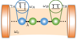
Figure 1: Scheme of a structure-engineered quantum battery architecture consisting a cavity and a working substance–a dimeric spin lattice with staggered energy gaps $\omega_{A,B}$ and decay rates $\gamma_{A,B}$. Nearest-neighbor dipole-dipole couplings $\lambda$ is assumed uniform. In the storage phase, the dimeric spin lattice is decoupled from the cavity (frequency $\omega_{c}$), whereas in the charging and discharging phases the light-matter interaction is turned on and the cavity serves as a charger Ferraro et al. (2018); Andolina et al. (2018, 2019a); Quach et al. (with possible external driving fields) and a superradiant decay channel for spins Pirmoradian and Mølmer (2019), respectively.

Exploiting analytical solutions of quantum Lindblad master equation Lindblad (1976) available for the single-excitation sector of the Hilbert space, we confirm the cooperation of spin-spin correlations in spin population dynamics in an engineered QB, leading to a slower spin decaying pattern. On the contrary, spin population dynamics in the non-engineered counterpart exhibits a fast exponential decay trend. From the energetics, quantified by the stored total energy, we further show that an engineered QB significantly outperforms its non-engineered counterpart, with more energy preserved during the storage phase. In particular, we find that the relative energy gain is independent of system size, indicating that we achieved a scale-invariant protection with potential applications to future scalable quantum battery setups.

Microscopic model.–We consider a spin-cavity architecture (see Fig. 1 for a sketch) in light of existing theoretical proposals Ferraro et al. (2018); Andolina et al. (2018, 2019a); Pirmoradian and Mølmer (2019), and a recent experimental work Quach et al. . The QB model includes a one-dimensional spin-$1/2$ lattice as the working substance with spin gaps $\{\omega_{j}\}$, Pauli spin operators $\{\sigma_{j}^{z,\pm}\}$ ($\sigma_{j}^{-}=(\sigma_{j}^{+})^{\dagger}$), $j\in[1,\cdots,N]$ (setting $N$ an even number), and nearest-neighbor dipole-dipole interactions measured by the strength $\lambda$. The spins are coupled to an optical cavity supporting a single dispersionless mode with frequency $\omega_{c}$ and annihilation operator $a$. The light-matter coupling, measured by strength $\eta$, is treated within the rotating-wave-approximation. In the rotating frame, we obtain the total Hamiltonian (setting $\hbar=1$),

$$H_{\mathrm{tot}}\leavevmode\nobreak\ =\leavevmode\nobreak\ \sum_{j=1}^{N}\frac{\Delta_{j}}{2}\sigma_{j}^{z}+\sum_{j=1}^{N-1}\lambda(\sigma_{j}^{+}\sigma_{j+1}^{-}+\mathrm{H.c.})+\eta\sum_{j=1}^{N}(\sigma_{j}^{-}a^{\dagger}+\mathrm{H.c.}).$$ (1)

Here, $\Delta_{j}=\omega_{j}-\omega_{c}$, ‘H.c’ is short for ‘Hermitian conjugate’. Our results in the storage phase do not depend on the frequency $\omega_{c}$ itself.

In addition to the coherent Hamiltonian $H_{\mathrm{tot}}$, incoherent processes affect the QB. These include the decay of the intensity of the field within the cavity, with a rate constant $\kappa$, and the spontaneous decay of spins, with rate constants $\gamma_{j}$. In the weak dissipation regime of $\gamma_{j}\ll\Delta_{j}$, $\kappa\ll\omega_{c}$, the total density matrix $\rho_{\mathrm{tot}}$ of the cavity and spins is governed by the following Lindblad master equation Lindblad (1976) (explicit time dependence is suppressed)

$$\frac{\partial}{\partial t}\rho_{\mathrm{tot}}\leavevmode\nobreak\ =\leavevmode\nobreak\ -i[H_{\mathrm{tot}},\rho_{\mathrm{tot}}]+\kappa\mathcal{L}[a]\rho_{\mathrm{tot}}+\sum_{j=1}^{N}\gamma_{j}\mathcal{L}[\sigma_{j}^{-}]\rho_{\mathrm{tot}}.$$ (2)

Here, $\mathcal{L}[O]\rho_{\mathrm{tot}}=(2O\rho_{\mathrm{tot}}O^{\dagger}-O^{\dagger}O\rho_{\mathrm{tot}}-\rho_{\mathrm{tot}}O^{\dagger}O)/2$ denotes the Lindblad superoperator. We neglect dephasing and heating (incoherent pumping) of spins, as their rates can be made several orders of magnitude smaller than individual decay rates Schwager et al. (2013).

We limit our analysis to the storage phase. Following Ref. Pirmoradian and Mølmer (2019) we assume that the QB is fully charged (through the cavity Ferraro et al. (2018); Andolina et al. (2018, 2019a)) at time $t=0$ when the storage stage begins. During the storage stage we turn off the light-matter interaction by tuning the cavity frequency away from $\omega_{j}$. Hence, in the storage stage we just consider the reduced quantum master equation for spins (see the supplemental material SM for more details),

$$\frac{\partial}{\partial t}\rho_{S} = -i[H_{S},\rho_{S}]+\sum_{j=1}^{N}\gamma_{j}\mathcal{L}[\sigma_{j}^{-}]\rho_{S}\leavevmode\nobreak\ \equiv\leavevmode\nobreak\ \mathbb{L}\rho_{S}.$$ (3)

Here, $H_{S}=\sum_{j=1}^{N}\frac{\Delta_{j}}{2}\sigma_{j}^{z}+\sum_{j=1}^{N-1}\lambda(\sigma_{j}^{+}\sigma_{j+1}^{-}+\sigma_{j+1}^{+}\sigma_{j}^{-})$ is the spin lattice Hamiltonian in the rotating frame, $\mathbb{L}$ is the total Liouvillian.

Structure engineering scheme.– We begin with dynamical equations for spin population $\langle\sigma_{z}^{j}\rangle$ obtained using Eq. (3),

$$\frac{d}{dt}\langle\sigma_{j}^{z}\rangle = -2i\lambda\Big{[}\langle\sigma_{j}^{+}\sigma_{j+1}^{-}\rangle+\langle\sigma_{j}^{+}\sigma_{j-1}^{-}\rangle-\langle\sigma_{j+1}^{+}\sigma_{j}^{-}\rangle$$ (4)

$$-\langle\sigma_{j-1}^{+}\sigma_{j}^{-}\rangle\Big{]}-\gamma_{j}\langle 1+\sigma_{j}^{z}\rangle.$$

For long spin lattices with $N\gg 1$, we can neglect boundary effects and focus on the bulk of the QB. We observe that the first four terms, representing spin-spin correlations, cancel out exactly in the bulk of a uniform spin lattice with a translational invariance since, for instance, $\langle\sigma_{j-1}^{+}\sigma_{j}^{-}\rangle=\langle\sigma_{j}^{+}\sigma_{j+1}^{-}\rangle$. As a result, even though spin-spin correlations are nonzero, the spin population of a uniform spin lattice decays exponentially and locally, in the sense that the decaying dynamics is independent of other spins, leading to an aging of charged QBs Pirmoradian and Mølmer (2019).

Can one harness spin-spin correlations to mitigate aging? We answer this question affirmatively by introducing a strategy based on SE, building solely on the modulation of spin energy gaps such that, for instance, we should at least have $\Delta_{j}\neq\Delta_{j\pm 1}$ in the present model. Through SE, realized here with the addition of non-homogeneity of spin energy gaps to the otherwise uniform lattice, we break the translation invariance of the bulk such that $\langle\sigma_{j-1}^{+}\sigma_{j}^{-}\rangle\neq\langle\sigma_{j}^{+}\sigma_{j+1}^{-}\rangle$, resulting in nonzero contributions from spin-spin correlations to the spin population dynamics. The result of the inclusion of spin-spin correlations is that we can alter the decaying pattern of spin populations from a fast exponential trend to a non-exponential one. More intriguingly, the SE simultaneously modifies the spontaneous emission rate $\gamma_{j}$ as it is proportional to the spin energy gap (see, e.g., Ref. Lodahl et al. (2015)). Hence the engineered decay dynamics can become relatively slower, thereby mitigating aging effect in a passive manner.

Although here we lay out the SE scheme by focusing on a spin lattice with nearest-neighbor couplings, we emphasize that our SE scheme is not limited to this specific case. In fact, SE strategies can be tailored for other spin lattice models by inspecting the detailed form of the dynamical equations governing spin population dynamics, which is model dependent; more discussions will be provided later.

Dimeric lattice and single-excitation sector.–To facilitate the analysis with numerical insights, we adopt a dimeric SE: A dimeric spin lattice with staggered energy gaps $\Delta_{A,B}$ and decay rates $\gamma_{A,B}$ ($\gamma_{A}/\Delta_{A}=\gamma_{B}/\Delta_{B}$) but uniform dipole-dipole coupling strength $\lambda$ (see Fig. 1) . Without loss of generality, we set $\Delta_{j}=\Delta_{A(B)}$ if $j$ is odd (even). We note that a dimeric SE can either speed or slow the decay dynamics of the spin populations, compared to that of the non-engineered lattice ($\Delta_{A}=\Delta_{B}$), depending on the ratio $\Delta_{B}/\Delta_{A}$. For our purposes, we refer to the system with $\Delta_{A}=\Delta_{B}$ ($\Delta_{A}>\Delta_{B}$) as the non-engineered (engineered) QB.

We first focus on the single-excitation sector of the spin Hilbert space containing one spin excitation in total. Notably, the slowest decay dynamics of the system belongs to this sector Torres (2014); Cabot et al. (2019). Since the jump term $\sum_{j}\gamma_{j}\sigma_{j}^{-}\rho_{S}\sigma_{j}^{+}$ of the Lindblad master equation Eq. (3) does not contribute in this sector, the dissipative dynamics is fully governed by the part $\partial\rho_{S}/\partial t=\mathcal{K}\rho_{S}\equiv-i[K\rho_{S}-\rho_{S}K^{\dagger}]$ with an effective (non-Hermitian) Hamiltonian $K\equiv H_{S}-i\sum_{j}\frac{\gamma_{j}}{2}\sigma_{j}^{+}\sigma_{j}^{-}$. Since $K$ is quadratic, one easily finds its two-band complex eigenvalues under an open boundary condition Cabot et al. (2019) $\Omega_{k}^{\pm}\leavevmode\nobreak\ =\leavevmode\nobreak\ [(\Omega_{A}+\Omega_{B})/2]\pm\frac{1}{2}\sqrt{(\Omega_{A}-\Omega_{B})^{2}+16\lambda^{2}\cos^{2}(k/2)}$. Here, $\Omega_{A(B)}=\Delta_{A(B)}-i\gamma_{A(B)}$ and $k=2\pi l/(N+1)$ with $l=1,2,\cdots,N/2$. The eigenvalues of $K^{\dagger}$ are the complex conjugates $\Omega_{k}^{\pm\ast}$. In general, the eigenvalues of the Liouvillian $\mathbb{L}$ can be constructed by using $\Omega_{k}^{\pm}$ and $\Omega_{k}^{\pm\ast}$ as detailed in Ref. Torres (2014), while the smallest decay rates are $-\mathrm{Im}[\Omega_{k}^{\pm}]$ with ‘Im’ taking imaginary part. For a uniform lattice with $\Omega_{A}=\Omega_{B}$, we have $-\mathrm{Im}[\Omega_{k}^{\pm}]=\gamma_{A}$. Notably, the inverse of $\gamma_{A}$ sets the storage timescale for the non-engineered QB Pirmoradian and Mølmer (2019). On the contrary, we find that the smallest decay rates of the dimeric spin lattice is smaller than that of the uniform lattice (see the supplemental material SM ), indicating a longer storage time.

To quantify the dynamical behavior, we study spin populations $\langle\sigma_{j}^{z}(t)\rangle$ and spin-spin correlations $\langle\sigma_{j}^{+}(t)\sigma_{j^{\prime}}^{-}(t)\rangle$, which have the following analytical expressions in the single-excitation sector Cabot et al. (2019),

$$\langle\sigma_{j}^{z}(t)\rangle\leavevmode\nobreak\ =\leavevmode\nobreak\ 2\sum_{n,m}G_{n,m}(j)e^{-i(\Omega_{n}-\Omega_{m}^{\ast})t}-1,$$

$$\langle\sigma_{j}^{+}(t)\sigma_{j^{\prime}}^{-}(t)\rangle\leavevmode\nobreak\ =\leavevmode\nobreak\ \sum_{n,m}W_{n,m}(j,j^{\prime})e^{-i(\Omega_{n}-\Omega_{m}^{\ast})t}.$$ (5)

Here, $\Omega_{n}$ with $n$ running from $1$ to $N$ are elements of a $1\times N$ vector $\bm{\Omega}$ whose first (second) half belongs to $\Omega_{k}^{-}$ ($\Omega_{k}^{+}$) with $k$ running from $2\pi/(N+1)$ to $\pi N/(N+1)$ (see above). The coefficients $G_{n,m}(j)$ and $W_{n,m}(j,j^{\prime})$ are determined by the eigenvectors of $K$ and $K^{\dagger}$, as well as by the initial condition $\rho_{S}(0)$; we relegate their detailed expressions to the supplemental material SM .

In Fig. 2, we present results for population $\langle\sigma_{j}^{z}(t)\rangle$ and spin-spin correlation $\langle\sigma_{j}^{+}(t)\sigma_{j^{\prime}}^{-}(t)\rangle$ at the bulk of the spin chain (sites $j=10$ and $j=11$). We use Eq. (Boosting quantum battery performance by structure engineering) and assume the (arbitrary) initial state $\rho_{S}(0)=|\Phi_{0}\rangle\langle\Phi_{0}|$; $|\Phi_{0}\rangle=|g\rangle/\sqrt{2}+(|e_{j=10}\rangle+|e_{j=12}\rangle)/2$ with $|e_{j}\rangle=\sigma_{j}^{+}|g\rangle$ and $|g\rangle$ the global ground state of the spins, namely, $\sigma_{j}^{z}|g\rangle=-|g\rangle$. We confirmed that basic features depicted in Fig. 2 are independent of the initial condition adopted in the single-excitation sector.

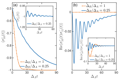
Figure 2: (a) Trajectory of $\langle\sigma_{10}^{z}(t)\rangle$ in a single-excitation sector using Eq. (Boosting quantum battery performance by structure engineering) for $\Delta_{B}/\Delta_{A}=0.25$ (blue solid line) and $\Delta_{B}/\Delta_{A}=1$ (orange dash-dotted line). Inset: Trajectory of $\langle\sigma_{11}^{z}(t)\rangle$ for $\Delta_{B}/\Delta_{A}=0.25$. (b) Trajectory of the real (Re) part of the spin-spin correlation $\langle\sigma_{10}^{+}(t)\sigma_{11}^{-}(t)\rangle$ using Eq. (Boosting quantum battery performance by structure engineering) for $\Delta_{B}/\Delta_{A}=0.25$ (blue solid line) and $\Delta_{B}/\Delta_{A}=1$ (orange dash-dotted line). Inset: Trajectory of the imaginary (Im) part of the spin-spin correlation $\langle\sigma_{10}^{+}(t)\sigma_{11}^{-}(t)\rangle$. Other parameters are $N=50$, $\gamma_{A,B}/\Delta_{A,B}=0.05$, $\lambda=0.05\Delta_{A}$.

From Fig. 2 (a), it is evident that spin population in a uniform (non-engineered) lattice (dash-dotted line) decays initially in an exponential manner. In comparison, the spin population in a dimeric lattice (solid line) depicts a slower decay, dressed by an oscillatory behavior at short times. Moreover, by the time $\Delta_{A}t=25$, the excited state population in the uniform case is close to zero, while in the dimerized case by that time only 40$\%$ had decayed to the ground state.

Based on the SE scheme and Eq. (4), we naturally expect that transient oscillations of the spin population (see also the inset for a nearest-neighbor site) in the dimeric lattice arise from the spin-spin correlations. To verify whether this is the case, we turn to the spin-spin correlation result showed in Fig. 2 (b). For clarity and simplicity, we just depict $\langle\sigma_{10}^{+}(t)\sigma_{11}^{-}(t)\rangle$ in accordance with population results of Fig. 2 (a). From Fig, 2 (b), we immediately note that spin-spin correlations in the dimeric lattice oscillate with a period that is consistent with that inferred from spin population dynamics at short times, confirming that spin-spin correlations indeed affect spin population dynamics in the dimeric lattice. In comparison, although we have nonzero spin-spin correlations in a uniform lattice, its impact on spin population dynamics is negligible, in accordance with Eq. (4). Hence, from the dynamics in the single-excitation sector, we confirm that SE (i) allows for the participation of spin-spin correlation in spin population dynamics, and (i) leads to slower decaying trend of spin populations, thereby mitigating the aging effect.

Energetics in the storage phase.– To characterize the performance of a fully-charged engineered QB, we turn to the energetics in the storage phase. This requires information of higher-order excitation sectors as we have $N$ excitations at $t=0$ ($\langle\sigma_{j}^{z}(t=0)\rangle=1$ but spin coherences and correlations are set to zero), namely, the full Lindblad master equation Eq. (3) should be utilized. We consider the dynamics of the average total energy normalized by frequencies,

$$\mathcal{E}(t)\equiv\frac{\langle H_{S}(t)\rangle}{\sum_{j=1}^{N}\Delta_{j}/2}.$$ (6)

This measure allows for a proper comparison between engineered and non-engineered QBs. It has been demonstrated for spin-based QBs that the average total energy approaches the ergotropy–the maximal extractable work under a cyclic unitary transformation Allahverdyan et al. (2004)–in the large $N$ limit Rossini et al. (2019); Andolina et al. (2019a); Quach and Munro (2020). We thus perform simulations in this limit. We denote by $\mathcal{E}_{d(u)}(t)$ the average total energy in the dimeric (uniform) lattice. The dynamics of $\mathcal{E}(t)$ is obtained by solving Eq. (4) together with those for higher-order correlation terms based on Eq. (3); coupled equations of motion obtained under a second-order cumulant approximation Xu et al. (2014); Meiser and Holland (2010) applicable for large $N$ are listed in the supplemental material SM .

In Fig. 3, we show the dynamics of the relative energy excess $[\mathcal{E}_{d}(t)-\mathcal{E}_{u}(t)]/\mathcal{E}_{u}(t)$ during the storage phase; a similar comparison for the averaged population is depicted in the supplemental material SM .

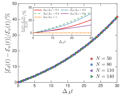
Figure 3: Dynamics of relative stored energy excess $[\mathcal{E}_{d}(t)-\mathcal{E}_{u}(t)]/\mathcal{E}_{u}(t)$ in the storage phase as a function of spin numbers $N$ with a fixed detuning ratio $\Delta_{B}/\Delta_{A}=0.25$. Inset: Relative excess energy when varying detuning ratio $\Delta_{B}/\Delta_{A}$ at a fixed number $N=80$. Other parameters are $\gamma_{A(B)}/\Delta_{A(B)}=0.05$ and $\lambda=0.05\Delta_{A}$.

We observe several features that are worth mentioning: (i) The engineered QB preserves more energy than the non-engineered counterpart as the storage time goes. Particularly, the relative excess $[\mathcal{E}_{d}(t)-\mathcal{E}_{u}(t)]/\mathcal{E}_{u}(t)$ is monotonic as a function of storage time. Approximately, we reveal the scaling $\mathcal{E}_{d}(t)/\mathcal{E}_{u}(t)\propto t^{\alpha}$ with $\alpha=1.5$ at long times SM . Notwithstanding, we point out that the absolute excess $\mathcal{E}_{d}(t)-\mathcal{E}_{u}(t)$ shows a turnover behavior when increasing the storage time SM , implying an optimal protection time for the engineered QB. Notably, one can also infer this property from Fig. 2 (a) for the population dynamics in the one-excitation sector, identified by the maximum population contrast appears around $\Delta_{A}t\sim 30$. (ii) The relative excess is independent of the number of spins $N$, indicating that the resulting passive protection scheme is scale-invariant and can be applied to large-scale QBs. (iii) The inset shows that the relative excess is a nonmonotonic function in the frequency ratio $\Delta_{B}/\Delta_{A}$, with the maximum achieved at an intermediate value. This property indicates that the so-obtained advantage of engineered QBs is not merely a consequence of the modification of decay rates from $\gamma_{A}$ to $\gamma_{B}$ for spins with even indices, otherwise, we should have observed a monotonic dependence of the relative excess on the frequency ratio $\Delta_{B}/\Delta_{A}$ as $\gamma_{B}$ monotonically approaches $\gamma_{A}$ when we increase the ratio. We note that such a dimeric spin lattice allows for an intriguing collective spin motion, namely, quantum transient synchronization Cabot et al. (2019) as featured by decaying oscillations of spin coherences $\langle\sigma_{j}^{x}(t)\rangle$, with the same frequency, in spite of distinct intrinsic spin frequencies (see the supplemental material SM for trajectories with varying $\Delta_{B}/\Delta_{A}$). Interestingly, this synchronization only occurs within a specific range of frequency ratio Cabot et al. (2019); SM . We therefore argue that the observed nonmonotonic behavior in energy stored indicates that the nontrivial collective spin motion enabled by spin-spin correlations contributes to the advantage of engineered QBs.

Discussion.– We envision realization of the engineered QB using circuit QED architectures involving superconducting qubits Houck et al. (2012); Salathé et al. (2015); Müller et al. (2019); Carusotto et al. (2020); Blais et al. (2020); Burkard et al. (2020), leveraging an exquisite tunability over system parameters such as the qubit frequency. Furthermore, one can easily scale up the system size in circuit QED Kollár et al. (2019), allowing for scalable QB designs. The implementation of the engineered QB is not tied to circuit QED setups in light of parallel advances in a variety of other experimental platforms, including cold atoms Reitz et al. (2013); Goban et al. (2014); Douglas et al. (2016); Bernien et al. (2017), quantum dots Yalla et al. (2014); Arcari et al. (2014), and trapped ions Barreiro et al. (2011) in optical traps and photonic structures, where spins connected in a one-dimensional arrangement are concerned.

Two possible extensions of the present strategy to more complicated QB designs are anticipated: (i) Many-body QBs with long-range spin-spin couplings beyond nearest-neighbor order Le et al. (2018); Rossini et al. (2019). In this scenario, equations of motion for spin populations involve long-range correlation terms and we expect engineered structures beyond a dimeric configuration, depending on the details of the underlying spin-spin interaction pattern. (ii) QBs in higher dimensions. Taking a possible two-dimensional QB as an example, we anticipate that the same approach of SE would directly apply if we limit spin-spin interactions to lowest nearest-neighbor terms. Although experimental techniques for connecting spins in two-dimensional arrangements are mature Bloch et al. (2008, 2012), it is challenging to implement the dimeric lattice as it creates a certain spatial-ordered pattern with two kinds of spins. We defer those ideas to future studies.

In summary, we introduced a generic SE scheme applicable to spin-based QBs, obtained by inspecting the dynamical equations of motion for spin populations [cf. Eq. (4) for a lattice with nearest-neighbor couplings]. Through a modulation of spin energy gap, the engineered QB can harness spin-spin correlations to mitigate aging effect in the storage stage, thereby achieving an advantage in extending the longevity of charged QBs. We expect that the resulting scale-invariant protection strategy, which is applicable in noisy environments, to play a central role in boosting the performance of QBs.

Acknowledgement.– We thank Albert Cabot for insightful discussions and assistance in simulations, and Ilia Khait for critical reading of the manuscript. This work was supported by the Natural Sciences and Engineering Research Council (NSERC) of Canada Discovery Grant and the Canada Research Chairs Program.

Supplemental material: Boosting quantum battery performance by structure engineering

In this supplemental material, we analyze spin dynamics in the single-excitation sector, derive coupled equations of motion for spin operators, which govern the dynamics of quantum battery (QB) in the storage phase while taking into account many-excitation sectors, and present additional simulation results that complement those included in the main text.

I I. Dynamical evolution in the single-excitation sector

In the main text, we presented simulations for $\langle\sigma_{j}^{z}(t)\rangle$ and $\langle\sigma_{j}^{+}(t)\sigma_{j^{\prime}}^{-}(t)\rangle$ based on Eqs. (S8) and (S10) below, respectively. For completeness of our presentation, we cover here essential results from Ref. Cabot et al. (2019) to explain how these expressions are derived.

In the single-excitation sector, spin dynamics is fully governed by the master equation $\partial\rho_{S}/\partial t=\mathcal{K}\rho_{S}=-i(K\rho_{S}-\rho_{S}K^{\dagger})$ with $K=H_{S}-i\sum_{j}\frac{\gamma_{j}}{2}\sigma_{j}^{+}\sigma_{j}^{-}$ a quadratic effective Hamiltonian. To solve this master equation, one just needs the eigenspectrum of $K$. We place the eigenvalues in the vector $\bm{\Omega}=(\{\Omega_{n}\})$ and organize the right and left eigenvectors of $K$ in the matrices $\bm{M_{R}}=(\{|K_{n}\rangle\})$, $\bm{M_{L}}=(\{\langle K_{n}^{\ast}|\})$ respectively, with $n$ running from 1 to $N$. Resorting to the Jordan-Wigner transformation tailored for the single-excitation subspace, one finds the following eigenvalues

$$\bm{\Omega}\leavevmode\nobreak\ =\leavevmode\nobreak\ (\{\Omega_{k}^{-}\},\{\Omega_{k}^{+}\})=(\Omega_{1},\Omega_{2},\Omega_{3},\cdots,\Omega_{N}),$$ (S1)

where $\Omega_{k}^{\pm}$ is given by Cabot et al. (2019)

$$\Omega_{k}^{\pm}\leavevmode\nobreak\ =\leavevmode\nobreak\ \frac{\Omega_{A}+\Omega_{B}}{2}\pm\frac{1}{2}\sqrt{(\Omega_{A}-\Omega_{B})^{2}+16\lambda^{2}\cos^{2}(k/2)}.$$ (S2)

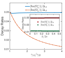
Figure S1: Decay rates $|\mathrm{Im}(\Omega_{k}^{+})|/\Delta_{A}$ (blue solid line) and $|\mathrm{Im}(\Omega_{k}^{-})|/\Delta_{A}$ (red dash-dotted line) of the one-excitation sector with varying ratio $\gamma_{A}/\gamma_{B}$ and a fixed $k=20\pi/(N+1)$. Inset: Decay rates $|\mathrm{Im}(\Omega_{k}^{+})|/\Delta_{A}$ (red circles) and $|\mathrm{Im}(\Omega_{k}^{-})|/\Delta_{A}$ (green squares) as a function of index $k=2\pi l/(N+1)$ ($l=1,2,\cdots,N/2$) with $\Delta_{B}=0.25\Delta_{A}$. The black solid line marks the uniform decay rate $|\mathrm{Im}(\Omega_{k}^{+})|=|\mathrm{Im}(\Omega_{k}^{-})|$ for the uniform lattice with $\Delta_{B}=\Delta_{A}$. Other parameters are $N=50$, $\gamma_{j}/\Delta_{j}=0.05$, $\lambda=0.05\Delta_{A}$.

$\Omega_{A(B)}=\Delta_{A(B)}-i\gamma_{A(B)}$ and $k=2\pi l/(N+1)$ with $l=1,2,\cdots,N/2$. The eigenvalues of $K^{\dagger}$ are the complex conjugates $\Omega_{k}^{\pm\ast}$. In general, the eigenvalues of the Liouvillian $\mathbb{L}$ can be constructed by using $\Omega_{k}^{\pm}$ and $\Omega_{k}^{\pm\ast}$ as detailed in Ref. Torres (2014). Interestingly, for the single-excitation sector with smallest decay rates, the corresponding eigenvalues of the Liouvillian $\mathbb{L}$ are $-i\Omega_{k}^{\pm}$ and $i\Omega_{k}^{\pm\ast}$. Hence, the absolute values of the imaginary parts of $\Omega_{k}^{\pm}$ set the decay rates of the slowest modes. As can be seen, for uniform spin lattice with $\gamma_{A}=\gamma_{B}\equiv\gamma_{0}$, we get $\Omega_{A}=\Omega_{B}$, hence the imaginary parts of $\Omega_{k}^{\pm}$ coincide, and take the value $\gamma_{0}$; for uniform QBs, $\gamma_{0}^{-1}$ sets the storage time scale Pirmoradian and Mølmer (2019). In contrast, for dimeric lattices with $\gamma_{A}\neq\gamma_{B}$, the intrinsic decay rates are modified. Noting that for vanishing dipole-dipole interactions, $\lambda=0$, we still have two bands provided that $\Omega_{A}\neq\Omega_{B}$. In Fig. S1, we present results for the decay rates $|\mathrm{Im}(\Omega_{k}^{\pm})|$ (‘Im’ takes imaginary part hereafter) for the slowest single-excitation sector. From Fig. S1 and its inset, we clearly observe that the engineered decay rates $|\mathrm{Im}(\Omega_{k}^{\pm})|$ of two bands in dimeric spin lattices can be made both smaller than that of the uniform limit ($\gamma_{A}=\gamma_{B}=0.05\Delta_{A}$ in present simulations), thereby implying a much longer storage time for a dimeric QB, as compared with its non-engineered counterpart.

The corresponding eigenvectors are expressed as Cabot et al. (2019)

$$\bm{M_{R}}\leavevmode\nobreak\ =\leavevmode\nobreak\ (\{v_{k}^{\prime}|g\rangle\},\{u_{k}^{\prime}|g\rangle\}),\leavevmode\nobreak\ \leavevmode\nobreak\ \bm{M_{L}}\leavevmode\nobreak\ =\leavevmode\nobreak\ (\{\langle g|v_{k}\},\{\langle g|u_{k}\}).$$ (S3)

Here, $|g\rangle$ is the global ground state of the spin lattice with $\sigma_{j}^{z}|g\rangle=-|g\rangle$. The operators $u_{k}^{\prime},\leavevmode\nobreak\ v_{k}^{\prime}$ are defined as

$$v_{k}^{\prime} = \sqrt{\frac{4}{N+1}}\sum_{m=1}^{N/2}\Big{(}\sigma_{2m-1}^{+}\sin\theta_{k}\sin[k(m-1/2)]+\sigma_{2m}^{+}\cos\theta_{k}\sin(km)\Big{)},$$

$$u_{k}^{\prime} = \sqrt{\frac{4}{N+1}}\sum_{m=1}^{N/2}\Big{(}\sigma_{2m-1}^{+}\cos\theta_{k}\sin[k(m-1/2)]-\sigma_{2m}^{+}\sin\theta_{k}\sin(km)\Big{)}.$$ (S4)

Here, $\theta_{k}$ is determined by $\tan 2\theta_{k}=-4\lambda\cos(k/2)/(\Delta_{A}-\Delta_{B}-i(\gamma_{A}-\gamma_{B}))$. Operators $v_{k}$ and $u_{k}$ are obtained from $v_{k}^{\prime}$ and $u_{k}^{\prime}$, by replacing spin raising operators with lowering ones, respectively.

In terms of the eigenvectors of the effective Hamiltonian $K$, we introduce the decomposition of the reduced system density matrix

$$\rho_{S}\leavevmode\nobreak\ =\leavevmode\nobreak\ \left(\sum_{nm}\mathcal{P}_{n,m}+\sum_{n}\mathcal{P}_{n,0}+\sum_{n}\mathcal{P}_{0,n}+\mathcal{P}_{0,0}\right)\rho_{S}.$$ (S5)

Here, $n,\leavevmode\nobreak\ m$ are indices running from 1 to $N$, we denote projectors as

$$\mathcal{P}_{n,m}\rho_{S} = \langle K_{n}^{\ast}|\rho_{S}|K_{m}^{\ast}\rangle|K_{n}\rangle\langle K_{m}|,$$

$$\mathcal{P}_{n,0}\rho_{S} = \langle K_{n}^{\ast}|\rho_{S}|g\rangle|K_{n}\rangle\langle g|,$$

$$\mathcal{P}_{0,n}\rho_{S} = \langle g|\rho_{S}|K_{n}^{\ast}\rangle|g\rangle\langle K_{n}|,$$

$$\mathcal{P}_{0,0}\rho_{S} = \langle g|\rho_{S}|g\rangle|g\rangle\langle g|.$$ (S6)

To illustrate the occurrence of quantum synchronization, we study the ensemble average $\langle\sigma_{j}^{x}(t)\rangle$,

$$\langle\sigma_{j}^{x}(t)\rangle = 2\mathrm{Re}\langle\sigma_{j}^{-}(t)\rangle\leavevmode\nobreak\ =\leavevmode\nobreak\ 2\mathrm{Re}\langle e_{j}|\rho_{S}(t)|g\rangle$$ (S7)

$$= 2\mathrm{Re}\langle e_{j}|\sum_{n}\mathcal{P}_{n,0}\rho_{S}(t)|g\rangle.$$

Here, $|e_{j}\rangle=\sigma_{j}^{+}|g\rangle$. It is easy to show that $\mathcal{P}_{n,0}\rho_{S}(t)=\mathcal{P}_{n,0}\rho_{S}(0)e^{-i\Omega_{n}t}$ using $\mathcal{K}|K_{n}\rangle\langle g|=-i\Omega_{n}|K_{n}\rangle\langle g|$, hence we have

$$\langle\sigma_{j}^{x}(t)\rangle\leavevmode\nobreak\ =\leavevmode\nobreak\ 2\mathrm{Re}\left[\sum_{n=1}^{N}F_{n}(j)e^{-i\Omega_{n}t}\right],$$ (S8)

with $F_{n}(j)=\langle K_{n}^{\ast}|\rho_{S}(0)|g\rangle\langle e_{j}|K_{n}\rangle$ and $\rho_{S}(0)=|\Phi_{0}\rangle\langle\Phi_{0}|$ ($|\Phi_{0}\rangle$ is the initial state). For our purpose, we also consider $\langle\sigma_{j}^{z}(t)\rangle$ in the single-excitation sector. Using Eq. (S5) and the relation $\mathcal{P}_{n,m}\rho_{S}(t)=\mathcal{P}_{n,m}\rho_{S}(0)e^{-i(\Omega_{n}-\Omega_{m}^{\ast})t}$, we immediately find that

$$\langle\sigma_{j}^{z}(t)\rangle\leavevmode\nobreak\ =\leavevmode\nobreak\ 2\langle e_{j}|\sum_{n,m}\mathcal{P}_{n,m}\rho_{S}(t)|e_{j}\rangle-1\leavevmode\nobreak\ =\leavevmode\nobreak\ 2\sum_{n=1,m=1}^{N}G_{n,m}(j)e^{-i(\Omega_{n}-\Omega_{m}^{\ast})t}-1.$$ (S9)

Here, $G_{n,m}(j)=\langle e_{j}|K_{n}\rangle\langle K_{m}|e_{j}\rangle\langle K_{n}^{\ast}|\rho_{S}(0)|K_{m}^{\ast}\rangle$ with $|K_{n}^{\ast}\rangle$ and $\langle K_{n}|$ the right and left eigenvectors of $K^{\dagger}$ with eigenvalues $\Omega_{n}^{\ast}$. Analogously, we obtain the following expression for spin-spin correlations $\langle\sigma_{j}^{+}(t)\sigma_{j^{\prime}}^{-}(t)\rangle$:

$$\langle\sigma_{j}^{+}(t)\sigma_{j^{\prime}}^{-}(t)\rangle = \langle e_{j^{\prime}}|\rho_{S}(t)|e_{j}\rangle$$ (S10)

$$= \sum_{n=1,m=1}^{N}W_{n,m}(j,j^{\prime})e^{-i(\Omega_{n}-\Omega_{m}^{\ast})t}$$

with $W_{n,m}(j,j^{\prime})=\langle K_{n}^{\ast}|\rho_{S}(0)|K_{m}^{\ast}\rangle\langle K_{m}|e_{j}\rangle\langle e_{j^{\prime}}|K_{n}\rangle$.

In Fig. S2, we present trajectories $\langle\sigma_{j}^{x}(t)\rangle$ using Eq. (S8) while varying the frequency ratio $\Delta_{B}/\Delta_{A}$. From this comparison, we observe that for relative small ratios $\Delta_{B}/\Delta_{A}$ a phase synchronization emerges at the trajectory level as the two trajectories depict almost perfect anti-phase oscillations, while when the ratio $\Delta_{B}/\Delta_{A}$ approaches unity, this anti-phase oscillation becomes obscure as can be seen from Fig. S2 (d), consistent with findings in Ref. Cabot et al. (2019) for short lattices.

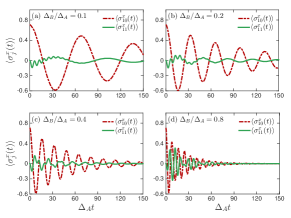
Figure S2: Trajectories for $\langle\sigma_{10}^{x}(t)\rangle$ (red dash-dotted line) and $\langle\sigma_{11}^{x}(t)\rangle$ (green solid line) using Eq. (S8) for a dimeric lattice while varying the detuning ratio $\Delta_{B}/\Delta_{A}$. (a) $\Delta_{B}/\Delta_{A}=0.1$, (b) $\Delta_{B}/\Delta_{A}=0.2$, (c) $\Delta_{B}/\Delta_{A}=0.4$, and (d) $\Delta_{B}/\Delta_{A}=0.8$. We adopt the initial state $|g\rangle/\sqrt{2}+(|e_{j=10}\rangle+|e_{j=12}\rangle)/2$. Other parameters are $N=50$, $\gamma_{j}/\Delta_{j}=0.05$, $\lambda=0.05\Delta_{A}$.

II II. Many excitations case: Dynamical equations for expectation values of spin operators

In this section, we first illustrate how to introduce a superradiant decay channel for spins in the discharging phase when the cavity is coupled to the spin chain. To this end, we consider the so-called bad cavity limit, $\kappa\gg\eta,\leavevmode\nobreak\ \gamma_{j}$ Pirmoradian and Mølmer (2019). In this limit, the cavity degrees of freedom can be adiabatically eliminated using the solution Xu et al. (2014)

$$a\leavevmode\nobreak\ \simeq\leavevmode\nobreak\ -\frac{2i\eta}{\kappa+i\Delta_{A}}J_{A}^{-}-\frac{2i\eta}{\kappa+i\Delta_{B}}J_{B}^{-},$$ (S11)

where $J_{A(B)}^{-}\equiv\sum_{j\in\mathrm{odd}(\mathrm{even})}\sigma_{j}^{-}$ are collective lowering spin operators. Noting that frequency detuning $\Delta_{A,B}=\omega_{A,B}-\omega_{c}$ can be made small relative to $\kappa$ for bad cavities, we simplify Eq. (S11) as $a\simeq-2i\eta J^{-}/\kappa$ with $J^{-}=J_{A}^{-}+J_{B}^{-}=\sum_{j}\sigma_{j}^{-}$, yielding

$$\frac{\partial}{\partial t}\rho_{S} = -i[H_{S},\rho_{S}]+\sum_{j=1}^{N}\gamma_{j}\mathcal{L}[\sigma_{j}^{-}]\rho_{S}+\Gamma\mathcal{L}[J^{-}]\rho_{S}.$$ (S12)

Here, $H_{S}=\sum_{j=1}^{N}\frac{\Delta_{j}}{2}\sigma_{j}^{z}+\sum_{j=1}^{N-1}\lambda(\sigma_{j}^{+}\sigma_{j+1}^{-}+\mathrm{H.c.})$ is the Hamiltonian of dimer spin lattice, $\Gamma=4\eta^{2}/\kappa$ denotes a Purcell-enhanced emission rate marking a cavity-induced superradiant process, which is designed to be the dominant decay channel for spins in the discharging phase. By setting $\Gamma=0$, we recover the quantum master equation used for analyzing the storage phase in the main text.

To derive dynamical equations from the master equation Eq. (S12), we use the relations $\mathrm{Tr}\{A[H_{S},\rho_{S}]\}=\mathrm{Tr}\{[A,H_{S}]\rho_{S}\}$ and

$$\mathrm{Tr}\{A\mathcal{L}[O]\rho_{S}\}\leavevmode\nobreak\ =\leavevmode\nobreak\ \frac{1}{2}\mathrm{Tr}\{[O^{\dagger},A]O\rho_{S}\}+\frac{1}{2}\mathrm{Tr}\{\rho_{S}O^{\dagger}[A,O]\}$$ (S13)

for an arbitrary spin operator $A$ and a Lindblad superoperator $\mathcal{L}[O]\rho_{S}=(2O\rho_{S}O^{\dagger}-O^{\dagger}O\rho_{S}-\rho_{S}O^{\dagger}O)/2$. The dynamical equation for $\langle\sigma_{j}^{z}\rangle$ takes the form (explicit time dependence is suppressed hereafter):

$$\frac{d}{dt}\langle\sigma_{j}^{z}\rangle = -2i\lambda\left[\langle\sigma_{j}^{+}\sigma_{j+1}^{-}\rangle+\langle\sigma_{j}^{+}\sigma_{j-1}^{-}\rangle-\langle\sigma_{j+1}^{+}\sigma_{j}^{-}\rangle-\langle\sigma_{j-1}^{+}\sigma_{j}^{-}\rangle\right]-\gamma_{j}\langle 1+\sigma_{j}^{z}\rangle$$ (S14)

$$-\Gamma\langle 1+\sigma_{j}^{z}\rangle-\Gamma\sum_{m\neq j}\Big{[}\langle\sigma_{j}^{+}\sigma_{m}^{-}\rangle+\mathrm{c.c.}\Big{]},$$

where ‘c.c’ denotes complex conjugate. From the above equation of motion, it is evident that the discharging phase always benefits from a superradiant decay channel with a Purcell-enhanced emission rate, $\Gamma\gg\gamma_{A,B}$, thereby achieving a fast discharging process Pirmoradian and Mølmer (2019). We highlight that our setup lacks a permutation symmetry, that is, spin correlations depend on the indices due to the presence of a nearest-neighbor dipole-dipole coupling, in contrast to the scenario studied in Ref. Pirmoradian and Mølmer (2019).

The above dynamical equation should be solved subject to those for $\langle\sigma_{n}^{+}\sigma_{m}^{-}\rangle$. Below we limit our attention to the storage phase when $\Gamma$ is tuned to zero. For $\langle\sigma_{n}^{+}\sigma_{m}^{-}\rangle$, we find it convenient to separately treat two scenarios, due to the presence of nearest-neighbor dipole-dipole coupling: (i) $m=n\pm 1$ and (ii) $m\neq n,n\pm 1$,

• Case (i):

  $$\frac{d}{dt}\langle\sigma_{n}^{+}\sigma_{n\pm 1}^{-}\rangle = \left[i(\Delta_{n}-\Delta_{n\pm 1})-\frac{\gamma_{n}+\gamma_{n\pm 1}}{2}\right]\langle\sigma_{n}^{+}\sigma_{n\pm 1}^{-}\rangle$$ (S15)

  $$-i\frac{\lambda}{2}\Big{[}\langle\sigma_{n}^{z}\rangle-\langle\sigma_{n\pm 1}^{z}\rangle\Big{]}-i\lambda\Big{[}\langle\sigma_{n}^{z}\sigma_{n\mp 1}^{+}\sigma_{n\pm 1}^{-}\rangle-\langle\sigma_{n\pm 1}^{z}\sigma_{n}^{+}\sigma_{n\pm 2}^{-}\rangle\Big{]}.$$

• Case (ii):

  $$\frac{d}{dt}\langle\sigma_{n}^{+}\sigma_{m}^{-}\rangle = \Big{[}i(\Delta_{n}-\Delta_{m})-\frac{\gamma_{n}+\gamma_{m}}{2}\Big{]}\langle\sigma_{n}^{+}\sigma_{m}^{-}\rangle$$ (S16)

  $$-i\lambda\sum_{h=n\pm 1}\langle\sigma_{n}^{z}\sigma_{m}^{-}\sigma_{h}^{+}\rangle+i\lambda\sum_{h=m\pm 1}\langle\sigma_{m}^{z}\sigma_{n}^{+}\sigma_{h}^{-}\rangle.$$

To form a closed set of coupled dynamical equations, we adopt a semiclassical cumulant approximation that is applicable to large spin numbers: correlations are expanded to second order. Particularly, here we approximate $\langle\sigma_{n}^{z}\sigma_{m}^{+}\sigma_{h}^{-}\rangle\approx\langle\sigma_{n}^{z}\rangle\langle\sigma_{m}^{+}\sigma_{h}^{-}\rangle$ Meiser and Holland (2010). By doing so, we neglect correlations of the type $\langle\sigma_{n}^{z}\sigma_{m}^{+}\rangle$ ($n\neq m$) Xu et al. (2014). Accordingly, we approximate Eqs. (S15) and (S16) as

• Case (i):

  $$\frac{d}{dt}\langle\sigma_{n}^{+}\sigma_{n\pm 1}^{-}\rangle \approx \left[i(\Delta_{n}-\Delta_{n\pm 1})-\frac{\gamma_{n}+\gamma_{n\pm 1}}{2}\right]\langle\sigma_{n}^{+}\sigma_{n\pm 1}^{-}\rangle-i\frac{\lambda}{2}\Big{[}\langle\sigma_{n}^{z}\rangle-\langle\sigma_{n\pm 1}^{z}\rangle\Big{]}$$ (S17)

  $$-i\lambda\Big{[}\langle\sigma_{n}^{z}\rangle\langle\sigma_{n\mp 1}^{+}\sigma_{n\pm 1}^{-}\rangle-\langle\sigma_{n\pm 1}^{z}\rangle\langle\sigma_{n}^{+}\sigma_{n\pm 2}^{-}\rangle\Big{]}.$$

• Case (ii):

  $$\frac{d}{dt}\langle\sigma_{n}^{+}\sigma_{m}^{-}\rangle \approx \left[i(\Delta_{n}-\Delta_{m})-\frac{\gamma_{n}+\gamma_{m}}{2}\right]\langle\sigma_{n}^{+}\sigma_{m}^{-}\rangle$$ (S18)

  $$-i\lambda\sum_{h=n\pm 1}\langle\sigma_{n}^{z}\rangle\langle\sigma_{h}^{+}\sigma_{m}^{-}\rangle+i\lambda\sum_{h=m\pm 1}\langle\sigma_{m}^{z}\rangle\langle\sigma_{n}^{+}\sigma_{h}^{-}\rangle.$$

Eqs. (S14), (S17) and (S18) form a closed set, which can be numerically propagated by means of, for instance, Runge-Kutta algorithm subject to the open boundary condition for the spin lattice.

III III. Additional simulation results

In this section, we include additional simulations that complement those shown in the main text. For characterizing the performance of QBs in the storage phase, one can also look at the normalized population defined as

$$\mathcal{P}(t)\leavevmode\nobreak\ =\leavevmode\nobreak\ \frac{\sum_{j=1}^{N}\frac{\Delta_{j}}{2}\langle\sigma_{j}^{z}(t)\rangle}{\sum_{j=1}^{N}\Delta_{j}/2}.$$ (S19)

Similarly to the main text, we denote by $\mathcal{P}_{d(u)}(t)$ the population of the dimeric (uniform) spin lattice. A typical set of results is presented in Fig. S3.

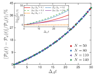
Figure S3: Dynamics of relative excess population $[\mathcal{P}_{d}(t)-\mathcal{P}_{u}(t)]/\mathcal{P}_{u}(t)$ in the storage phase as a function of spin number $N$ with a fixed detuning ratio $\Delta_{B}/\Delta_{A}=0.25$. The inset shows the relative excess energy when varying the detuning ratio $\Delta_{B}/\Delta_{A}$ and a fixed number of spins $N=80$. Other parameters are $\gamma_{A(B)}/\Delta_{A(B)}=0.05$ and $\lambda=0.05\Delta_{A}$.

As can be seen, the normalized population depicts almost the same behavior as the normalized energy shown in the main text. Therefore, the normalized population can also serve as a figure of merit for characterizing QBs in the storage phase.

In Fig. S4, we check the long time behavior of the absolute excess energy $\mathcal{E}_{d}(t)-\mathcal{E}_{h}(t)$.

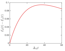
Figure S4: Dynamics of excess energy density $\mathcal{E}_{d}(t)-\mathcal{E}_{h}(t)$ in the storage phase for a dimeric battery with $\Delta_{B}/\Delta_{A}=0.25$. Other parameters are $N=80$, $\gamma_{j}/\Delta_{j}=0.05$, $\lambda=0.05\Delta_{A}$.

We find that $\mathcal{E}_{d}(t)-\mathcal{E}_{h}(t)$ depicts a turnover behavior when increasing the storage time, indicating that there is an optimal protection time for engineered QBs.

In Fig. S5, we analyze the dependence of $[\mathcal{E}_{d}(t)-\mathcal{E}_{u}(t)]/\mathcal{E}_{u}(t)$ on time. We observe a power-law behavior, $\mathcal{E}_{d}(t)/\mathcal{E}_{u}(t)\propto t^{\alpha}$, with $\alpha=1.5$ at longer times.

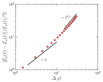
Figure S5: Dynamics of the relative stored energy excess $[\mathcal{E}_{d}(t)-\mathcal{E}_{u}(t)]/\mathcal{E}_{u}(t)$ as a function of time with a fixed detuning ratio $\Delta_{B}/\Delta_{A}=0.25$. Other parameters are $N=80$, $\gamma_{A(B)}/\Delta_{A(B)}=0.05$ and $\lambda=0.05\Delta_{A}$.

References

- Campaioli et al. (2018) F. Campaioli, F. A. Pollock, and S. Vinjanampathy, “Quantum batteries,” in Thermodynamics in the Quantum Regime: Recent Progress and Outlook, edited by F. Binder, L. A. Correa, C. Gogolin, J. Anders, and G. Adesso (Springer, 2018).
- Alicki and Fannes (2013) R. Alicki and M. Fannes, “Entanglement boost for extractable work from ensembles of quantum batteries,” Phys. Rev. E 87, 042123 (2013).
- Binder et al. (2015) F. C Binder, S. Vinjanampathy, K. Modi, and J. Goold, “Quantacell: powerful charging of quantum batteries,” New J. Phys. 17, 075015 (2015).
- Campaioli et al. (2017) F. Campaioli, F. A. Pollock, F. C. Binder, L. Céleri, J. Goold, S. Vinjanampathy, and K. Modi, “Enhancing the charging power of quantum batteries,” Phys. Rev. Lett. 118, 150601 (2017).
- Ferraro et al. (2018) D. Ferraro, M. Campisi, G. M. Andolina, V. Pellegrini, and M. Polini, “High-power collective charging of a solid-state quantum battery,” Phys. Rev. Lett. 120, 117702 (2018).
- Le et al. (2018) T. P. Le, J. Levinsen, K. Modi, M. M. Parish, and F. A. Pollock, “Spin-chain model of a many-body quantum battery,” Phys. Rev. A 97, 022106 (2018).
- Andolina et al. (2018) G. M. Andolina, D. Farina, A. Mari, V. Pellegrini, V. Giovannetti, and M. Polini, “Charger-mediated energy transfer in exactly solvable models for quantum batteries,” Phys. Rev. B 98, 205423 (2018).
- Liu et al. (2019) J. Liu, D. Segal, and G. Hanna, “Loss-free excitonic quantum battery,” J. Phys. Chem. C 123, 18303 (2019).
- Santos et al. (2019) A. C. Santos, B. Çakmak, S. Campbell, and N. T. Zinner, “Stable adiabatic quantum batteries,” Phys. Rev. E 100, 032107 (2019).
- Andolina et al. (2019a) G. Andolina, M. Keck, A. Mari, M. Campisi, V. Giovannetti, and M. Polini, “Extractable work, the role of correlations, and asymptotic freedom in quantum batteries,” Phys. Rev. Lett. 122, 047702 (2019a).
- Zhang et al. (2019) Y. Zhang, T. Yang, L. Fu, and X. Wang, “Powerful harmonic charging in a quantum battery,” Phys. Rev. E 99, 052106 (2019).
- Pirmoradian and Mølmer (2019) F. Pirmoradian and K. Mølmer, “Aging of a quantum battery,” Phys. Rev. A 100, 043833 (2019).
- Andolina et al. (2019b) G. M. Andolina, M. Keck, A. Mari, V. Giovannetti, and M. Polini, “Quantum versus classical many-body batteries,” Phys. Rev. B 99, 205437 (2019b).
- Farina et al. (2019) D. Farina, G. M. Andolina, A. Mari, M. Polini, and V. Giovannetti, “Charger-mediated energy transfer for quantum batteries: An open-system approach,” Phys. Rev. B 99, 035421 (2019).
- Rossini et al. (2020) D. Rossini, G. M. Andolina, D. Rosa, M. Carrega, and M. Polini, “Quantum advantage in the charging process of sachdev-ye-kitaev batteries,” Phys. Rev. Lett. 125, 236402 (2020).
- Rossini et al. (2019) D. Rossini, G. M. Andolina, and M. Polini, “Many-body localized quantum batteries,” Phys. Rev. B 100, 115142 (2019).
- Barra (2019) F. Barra, “Dissipative charging of a quantum battery,” Phys. Rev. Lett. 122, 210601 (2019).
- Hovhannisyan et al. (2020) K. V. Hovhannisyan, F. Barra, and A. Imparato, “Charging assisted by thermalization,” Phys. Rev. Research 2, 033413 (2020).
- Gherardini et al. (2020) S. Gherardini, F. Campaioli, F. Caruso, and F. C. Binder, “Stabilizing open quantum batteries by sequential measurements,” Phys. Rev. Research 2, 013095 (2020).
- Santos et al. (2020) A. C. Santos, A. Saguia, and M. S. Sarandy, “Stable and charge-switchable quantum batteries,” Phys. Rev. E 101, 062114 (2020).
- Quach and Munro (2020) J. Quach and W. Munro, “Using dark states to charge and stabilize open quantum batteries,” Phys. Rev. Applied 14, 024092 (2020).
- Bai and An (2020) S-Y. Bai and J-H. An, “Floquet engineering to reactivate a dissipative quantum battery,” Phys. Rev. A 102, 060201 (2020).
- Rosa et al. (2020) D. Rosa, D. Rossini, G. M. Andolina, M. Polini, and M. Carrega, “Ultra-stable charging of fast-scrambling sachdev-ye-kitaev quantum batteries,” J. High Energ. Phys. 2020, 67 (2020).
- Kamin et al. (2020) F. H. Kamin, F. T. Tabesh, S. Salimi, F. Kheirandish, and A. C Santos, “Non-markovian effects on charging and self-discharging process of quantum batteries,” New J. Phys. 22, 083007 (2020).
- (25) M. T. Mitchison, J. Goold, and J. Prior, “Charging a quantum battery with linear feedback control,” ArXiv:2012.00350.
- Ghosh et al. (2020) S. Ghosh, T. Chanda, and A. Sen(De), “Enhancement in the performance of a quantum battery by ordered and disordered interactions,” Phys. Rev. A 101, 032115 (2020).
- Caravelli et al. (2020) F. Caravelli, G. Coulter-De Wit, L. García-Pintos, and A. Hamma, “Random quantum batteries,” Phys. Rev. Research 2, 023095 (2020).
- (28) S. Bhattacharjee and A. Dutta, “Quantum thermal machines and batteries,” ArXiv:2008.07889.
- Blais et al. (2020) A. Blais, S. M. Girvin, and W. D. Oliver, “Quantum information processing and quantum optics with circuit quantum electrodynamics,” Nat. Phys. 16, 247 (2020).
- Burkard et al. (2020) G. Burkard, M. J. Gullans, X. Mi, and J. R. Petta, “Superconductor-semiconductor hybrid-circuit quantum electrodynamics,” Nat. Rev. Phys. 2, 129 (2020).
- (31) J. Q. Quach, K. E. McGhee, L. Ganzer, D. M. Rouse, B. W. Lovett, E. M. Gauger, J. Keeling, G. Cerullo, D. G. Lidzey, and T. Virgili, “An organic quantum battery,” ArXiv:2012.06026.
- Julià-Farré et al. (2020) S. Julià-Farré, T. Salamon, A. Riera, M. N. Bera, and M. Lewenstein, “Bounds on the capacity and power of quantum batteries,” Phys. Rev. Research 2, 023113 (2020).
- García-Pintos et al. (2020) L. P. García-Pintos, A. Hamma, and A. del Campo, “Fluctuations in extractable work bound the charging power of quantum batteries,” Phys. Rev. Lett. 125, 040601 (2020).
- Lindblad (1976) G. Lindblad, “On the generators of quantum dynamical semigroups,” Commun. Math. Phys. 48, 119 (1976).
- Schwager et al. (2013) H. Schwager, J. I. Cirac, and G. Giedke, “Dissipative spin chains: Implementation with cold atoms and steady-state properties,” Phys. Rev. A 87, 022110 (2013).
- (36) See Supplemental Material for details related to the dynamics in single-excitation sector, derivations of coupled dynamical equations of motion for spins and additional simulation results.
- Lodahl et al. (2015) P. Lodahl, S. Mahmoodian, and S. Stobbe, “Interfacing single photons and single quantum dots with photonic nanostructures,” Rev. Mod. Phys. 87, 347–400 (2015).
- Note (1) For systems with nearest-neighbor couplings, we note that a dimeric lattice is sufficient to break the translational invariance. However, one can consider more complicated structural engineering, for instance, a trimeric lattice.
- Torres (2014) J. M. Torres, “Closed-form solution of lindblad master equations without gain,” Phys. Rev. A 89, 052133 (2014).
- Cabot et al. (2019) A. Cabot, G. Giorgi, F. Galve, and R. Zambrini, “Quantum synchronization in dimer atomic lattices,” Phys. Rev. Lett. 123, 023604 (2019).
- Allahverdyan et al. (2004) A. E. Allahverdyan, R. Balian, and T. M. Nieuwenhuizen, “Maximal work extraction from finite quantum systems,” Europhys. Lett. 67, 565 (2004).
- Xu et al. (2014) M. Xu, D. A. Tieri, E. C. Fine, J. K. Thompson, and M. J. Holland, “Synchronization of two ensembles of atoms,” Phys. Rev. Lett. 113, 154101 (2014).
- Meiser and Holland (2010) D. Meiser and M. J. Holland, “Intensity fluctuations in steady-state superradiance,” Phys. Rev. A 81, 063827 (2010).
- Houck et al. (2012) A. A. Houck, H. E. T reci, and J. Koch, “On-chip quantum simulation with superconducting circuits,” Nat. Phys. 8, 292 (2012).
- Salathé et al. (2015) Y. Salathé, M. Mondal, M. Oppliger, J. Heinsoo, P. Kurpiers, A. Potočnik, A. Mezzacapo, U. Las Heras, L. Lamata, E. Solano, S. Filipp, and A. Wallraff, “Digital quantum simulation of spin models with circuit quantum electrodynamics,” Phys. Rev. X 5, 021027 (2015).
- Müller et al. (2019) C. Müller, J. H. Cole, and J. Lisenfeld, “Towards understanding two-level-systems in amorphous solids: insights from quantum circuits,” Rep. Prog. Phys. 82, 124501 (2019).
- Carusotto et al. (2020) I. Carusotto, A. Houck, A. Kollár, P. Roushan, D. Schuster, and J. Simon, “Photonic materials in circuit quantum electrodynamics,” Nat. Phys. , 268 (2020).
- Kollár et al. (2019) A. Kollár, M. Fitzpatrick, and A. Houck, “Hyperbolic lattices in circuit quantum electrodynamics,” Nature 571, 45 (2019).
- Reitz et al. (2013) D. Reitz, C. Sayrin, R. Mitsch, P. Schneeweiss, and A. Rauschenbeutel, “Coherence properties of nanofiber-trapped cesium atoms,” Phys. Rev. Lett. 110, 243603 (2013).
- Goban et al. (2014) A. Goban, C.-L. Hung, S.-P. Yu, J.D. Hood, J.A. Muniz, J.H. Lee, M.J. Martin, A.C. McClung, K.S. Choi, D.E. Chang, O. Painter, and H.J. Kimble, “Atom-light interactions in photonic crystals,” Nat. Commun. 5, 3808 (2014).
- Douglas et al. (2016) J. S. Douglas, T. Caneva, and D. E. Chang, “Photon molecules in atomic gases trapped near photonic crystal waveguides,” Phys. Rev. X 6, 031017 (2016).
- Bernien et al. (2017) H. Bernien, S. Schwartz, A. Keesling, H. Levine, A. Omran, H. Pichler, S. Choi, A. S. Zibrov, M. Endres, M. Greiner, V. Vuleti?, and M. D. Lukin, “Probing many-body dynamics on a 51-atom quantum simulator,” Nature 551, 579 (2017).
- Yalla et al. (2014) R. Yalla, M. Sadgrove, K. P. Nayak, and K. Hakuta, “Cavity quantum electrodynamics on a nanofiber using a composite photonic crystal cavity,” Phys. Rev. Lett. 113, 143601 (2014).
- Arcari et al. (2014) M. Arcari, I. Söllner, A. Javadi, S. Lindskov Hansen, S. Mahmoodian, J. Liu, H. Thyrrestrup, E. H. Lee, J. D. Song, S. Stobbe, and P. Lodahl, “Near-unity coupling efficiency of a quantum emitter to a photonic crystal waveguide,” Phys. Rev. Lett. 113, 093603 (2014).
- Barreiro et al. (2011) J. T. Barreiro, M. Müller, P. Schindler, D. Nigg, T. Monz, M. Chwalla, M. Hennrich, C. F. Roos, P. Zoller, and R. Blatt, “An open-system quantum simulator with trapped ions,” Nature 470, 486 (2011).
- Bloch et al. (2008) I. Bloch, J. Dalibard, and W. Zwerger, “Many-body physics with ultracold gases,” Rev. Mod. Phys. 80, 885 (2008).
- Bloch et al. (2012) I. Bloch, J. Dalibard, and S. Nascimbéne, “Quantum simulations with ultracold quantum gases,” Nat. Phys. 8, 267 (2012).