Topological correlators of $SU(2)$, $\mathcal{N}=2^{*}$ SYM on four-manifolds

Abstract:

We consider topologically twisted $\mathcal{N}=2$, $SU(2)$ gauge theory with a massive adjoint hypermultiplet on a smooth, compact four-manifold $X$. A consistent formulation requires coupling the theory to a ${\rm Spin}^{c}$ structure, which is necessarily non-trivial if $X$ is non-spin. We derive explicit formulae for the topological correlation functions when $b_{2}^{+}\geq 1$. We demonstrate that, when the ${\rm Spin}^{c}$ structure is canonically determined by an almost complex structure and the mass is taken to zero, the path integral reproduces known results for the path integral of the $\mathcal{N}=4$ gauge theory with Vafa-Witten twist. On the other hand, we reproduce results from Donaldson-Witten theory after taking a suitable infinite mass limit.

The topological correlators are functions of the UV coupling constant $\tau_{\rm uv}$ and we confirm that they obey the expected $S$-duality transformation laws. The holomorphic part of the partition function is a generating function for the Euler numbers of the matter (or obstruction) bundle over the instanton moduli space. For $b_{2}^{+}=1$, we derive a non-holomorphic contribution to the path integral, such that the partition function and correlation functions are mock modular forms rather than modular forms.

We comment on the generalization of this work to the large class of $\mathcal{N}=2$ theories of class $S$.

1 Introduction

This paper investigates applications of supersymmetric quantum field theory (SQFT) to the differential topology of four-dimensional manifolds. The story of the relation of SQFT and four-manifold topology is one of the paradigmatic examples of the interplay between mathematics and questions raised by fundamental physics, a subject sometimes called physical mathematics. Indeed the invention of topological quantum field theory (TQFT) by Witten was motivated by the desire to give a QFT interpretation of the Donaldson invariants [1]. The desire to use the SQFT interpretation to give an effective evaluation of the Donaldson invariants was in turn one of the motivations for the ground-breaking work of Seiberg and Witten on the low-energy dynamics of SQFT with $\mathcal{N}=2$ supersymmetry [2, 3]. (We henceforth refer to such theories as $d=4,\mathcal{N}=2$ theories.) The discoveries of Seiberg and Witten led to the formulation of the Seiberg-Witten invariants of four-manifolds, culminating in the formulation of the Witten conjecture expressing the Donaldson invariants in terms of the Seiberg-Witten invariants [4]. (For a complete derivation of the Witten conjecture using ideas from quantum field theory see [5].)

Witten’s original application of SQFT to Donaldson invariants made use of “pure” $\mathcal{N}=2$ supersymmetric Yang-Mills (SYM) with a nonabelian gauge group of rank one, where the adjective “pure” means that the field content consists entirely of a vectormultiplet. However, the general twisting procedure of [1] can in principle be applied to any $d=4,\mathcal{N}=2$ field theory and it can be interesting to investigate other such theories. (For much more about this general point, see Section 8 below.) The present paper focuses on the extension to $d=4,\mathcal{N}=2$ rank one SYM with an adjoint-valued hypermultiplet with $\mathcal{N}=2$ preserving mass term, a theory sometimes referred to as the $\mathcal{N}=2^{*}$ theory. We carry out a detailed investigation of the topological correlators of this theory on a certain class of four-manifolds $X$.

Throughout this paper $X$ will be a smooth, compact, oriented four-dimensional manifold without boundary. For simplicity we will assume $X$ is simply connected, although this condition could certainly be relaxed. Let $b_{2}^{+}$ denote the dimension of the maximal positive definite subspace of $H^{2}(X,\mathbb{R})$ under the intersection pairing. We will assume that $b_{2}^{+}$ is positive and odd. When $b_{2}^{+}$ is even and positive the topological correlators all vanish. When $b_{2}^{+}=0$ important new considerations enter the story which are beyond the scope of this paper. It is worth noting that the manifolds in the above class always admit an almost complex structure (ACS). (For a detailed explanation see Section 10.1 of [6].)

In order to formulate the topological correlators of the twisted $\mathcal{N}=2^{*}$ theory we will need the following four pieces of data:

1. An “ultraviolet coupling.” Mathematically this is encoded in a point $\tau_{\rm uv}\in\mathbb{H}$, the upper half of the complex plane. Following standard definitions we will denote $q_{\rm uv}:=e^{2\pi{\rm i}\tau_{\rm uv}}$.

2. A “mass parameter” $m\in\mathbb{C}$ and a “UV scale” $\Lambda\in\mathbb{C}$. These quantities enter the topological correlators only through the dimensionless ratio $t:=m/\Lambda$.

3. An “ultraviolet” ${\rm Spin}^{c}$-structure $\mathfrak{s}_{\rm uv}$ on $X$ endowed with ${\rm Spin}^{c}$ connection. The invariants only depend on this data through the characteristic class of $\mathfrak{s}_{\rm uv}$, denoted $c_{\rm uv}\in H^{2}(X,\mathbb{Z})$.

4. A “homology orientation,” that is, an orientation on $H^{2}(X,\mathbb{R})$. (Physically, this is used to orient the Berezinian of fermion zero modes.)

We use the adjective “ultraviolet” to characterize the ${\rm Spin}^{c}$-structure $\mathfrak{s}_{\rm uv}$ because (as was noted long ago [7]) the presence of adjoint-valued hypermultiplet fields in the $\mathcal{N}=2^{*}$ theory requires a choice of ${\rm Spin}^{c}$-structure in order to formulate a well-defined topologically twisted theory. This ${\rm Spin}^{c}$-structure will play a very important role in this paper. It should be distinguished from the “infrared” ${\rm Spin}^{c}$-structures that appear in the LEET evaluation of the path integral. For example in the Witten conjecture, and its generalizations discussed below the result is expressed as a sum over infrared ${\rm Spin}^{c}$-structures.

A generating function for the topological correlators can be written as a formal power series of polynomial functions on the homology $H_{*}(X,\mathbb{C})$. See equation (2) below. Formal path integral arguments suggest that, while the formulation of the QFT path integral makes use of a choice of Riemannian metric on $X$, nevertheless, the result of the QFT path integral should be independent of this choice of metric. Thus, formally, the topological correlators should be smooth manifold invariants, much like the Donaldson invariants. However, careful analysis reveals that the alleged metric-independence is not quite true: The path integral argument only guarantees that the variation of the path integral with respect to the metric is an integral over field space of a total derivative. There can be “BRST anomalies” when the boundary contribution is nonzero. For $b_{2}^{+}>1$ the invariants really are metric independent, but for $b_{2}^{+}=1$ there is metric dependence. The dependence enters only through the period point $J\in H^{2}(X,\mathbb{R})$. The period point $J$ is defined to be the unique class in the forward light cone of $H^{2}(X,\mathbb{R})$ which satisfies $J=*J$ and $J^{2}=1$. (The use of the forward light cone here is one place where the homology orientation enters in the expressions.) The dependence on $J$ turns out to be not a bug, but a feature. It is crucial in the derivation of the formulae for the invariants for manifolds with $b_{2}^{+}>1$, as explained in Section 7.

The topological correlators we study have a mathematical definition in terms of intersection theory on a moduli space of equations that generalize both the instanton and the Seiberg-Witten equations. We will now explain this in some detail. The relevant equations are the “nonabelian (adjoint) monopole equations” or the “nonabelian Seiberg-Witten equations.” Their relevance in our context was already noted long ago [7, 8]. To formulate the invariants we choose a principal $SO(3)$ bundle $P\to X$ with connection. Since $X$ has a ${\rm Spin}^{c}$ structure $\mathfrak{s}_{\rm uv}$ there is an associated rank 2 bundle $W^{+}\to X$ of chiral spinors and we choose a section $M\in\Gamma(W^{+}\otimes{\rm ad}P)$. There is a natural ${\rm Spin}^{c}$-Dirac operator acting on $M$ and the nonabelian monopole equations state that $M$ satisfies the Dirac equation while the self-dual curvature $F^{+}$ is equal to the hyperkähler moment map of the action of the group of gauge transformations on $W^{+}\otimes{\rm ad}P$. See (102) below for the precise statement.

We note in passing that if we choose the ${\rm Spin}^{c}$ structure $\mathfrak{s}_{\rm uv}$ to be the one canonically determined by an ACS then the adjoint-Seiberg-Witten equations are closely related to the renowned Vafa-Witten (VW) equations. The VW equations are equations for a gauge connection on $P$ together with a section $C\oplus B^{+}$ of $(L\oplus\Lambda^{2,+}T^{*}X)\otimes{\rm ad}P$ where $L$ is the trivial real line bundle. The essential observation is that, given an ACS, there is a canonical isomorphism $\Lambda^{2,+}T^{*}X\cong L\oplus K_{\mathbb{R}}$ where $K_{\mathbb{R}}$ is the underlying real 2-plane bundle of the canonical bundle $K$. On the other hand, one also has the natural isomorphism $W^{+}\cong L\otimes\mathbb{C}\oplus K$. In this way we can identify the fields $C,B^{+}$ of the VW theory with the monopole fields $M$. For a Kähler manifolds, the standard VW equation $D_{\mu}C+D^{\nu}B^{+}_{\mu\nu}=0$ is then equivalent to the Spin^c Dirac equation, and the equations for the curvature become isomorphic as well. For an almost complex manifold, we find that the nonabelian Seiberg-Witten equations are equivalent to a deformation of the standard VW equations. The deformation involves a compact perturbation of the Vafa-Witten operator $d\oplus d^{\dagger}$ by a term involving the Nijenhuis tensor. Based on the explicit results of this paper, we have reasons to believe that the solution spaces of the original and deformed VW equations give rise to the same topological invariants.

Returning to the mathematical formulation of the invariants we recall that the isomorphism class of the bundle $P$ is determined by the instanton number $k$ (see equation (121) for our normalization of the instanton number) and the “’t Hooft flux” $\nu:=w_{2}(P)$. Let $\mathcal{M}_{k,\nu,\mathfrak{s}}$ denote the moduli space (stack) of solutions to the nonabelian monopole equations. There is a Donaldson-type $\mu$ map:

$$\mu:H_{*}(X)\to H^{4-*}(\mathcal{M}_{k,\nu,\mathfrak{s}})$$ (1)

and the mathematical definition of the generating function for the topological correlators is of the form

$$Z_{\nu}(x;\tau_{\rm uv},c_{\rm uv},t):=\sum_{k\geq 0}q_{\rm uv}^{k}\int_{\mathcal{M}_{k,\nu,\mathfrak{s}}}e^{\mu(x)}\,{\rm Eul}(\mathcal{E}_{\mathfrak{s}};t),$$ (2)

where $x\in H_{*}(X,\mathbb{C})$ and ${\rm Eul}(\mathcal{E}_{\mathfrak{s}};t)$ is the $U(1)$-equivariant Euler class of a certain virtual bundle over the moduli space (stack) $\mathcal{M}_{k,\nu,\mathfrak{s}}$ (with equivariant parameter $t$). Here we are using a natural $U(1)$ symmetry of the nonablian monopole equations that rotates the monopole field by a phase. One arrives at the expression (2) by localization arguments, starting with the path integral of the twisted theory. See Section 3.6 for some more details. The basic elements of the argument can be found in [1, 8, 9, 10, 11, 12]. It must be said that giving a proper and careful mathematical definition of the intersection numbers in (2) is beyond the scope of this paper, and is a task best left to experts on the theory of moduli spaces. Among other things, one needs to orient ${\cal M}_{k,\nu,\mathfrak{s}}$. (For an ACS it will have a canonical orientation.) Indeed, already for projective surfaces, a careful definition of the VW invariants (which, we have explained, are a special case of our expressions) is a nontrivial and delicate mathematical problem [13, 14].

In this paper we will give very explicit formulae for (2). For the case $b_{2}^{+}>1$, the final results can be found in Section 7. They are given as a sum of three expressions, each of which is a sum over (infrared) ${\rm Spin}^{c}$-structures. The three expressions are Equations (427), (436) and (444) when $x=0$. The rules for including the dependence on $x$ are summarized in Tables 5 and 6. Upon specialization of the ${\rm Spin}^{c}$ structure, we find agreement with results in the physics literature [15, 16, 17]. In the $m\to\infty$ limit, we reproduce the Witten conjecture [4] from the perspective of $\mathcal{N}=2^{*}$ theory. In addition we find a very interesting connection to the recent mathematical works [18, Appendix C][19, 20]. These papers considered the addition of observables to the VW partition function for smooth projective surfaces with $h^{2,0}>0$. Our expressions for the path integral (derived in a completely independent way) are in precise agreement with those mathematical papers, as discussed in detail in Section 7. See especially Table 7.

The key to the derivation of the results of Section 7 is the so-called $u$-plane integral or Coulomb branch (CB) integral. This integral appears when discussing the invariants for the case $b_{2}^{+}=1$. When $b_{2}^{+}=1$ the full expression for the invariants derived from the path integral is of the form

$$Z_{\nu}^{J}(x;\tau_{\rm uv},c_{\rm uv},t)=\Phi_{\nu}^{J}+\sum_{j=1}^{3}Z^{J}_{SW,\nu,j}$$ (3)

where $\Phi_{\nu}^{J}$ is the CB integral and $Z^{J}_{SW,\nu,j}$ is the “Seiberg-Witten contribution” arising from singularities in the Coulomb branch measure at the point $u_{j}$ of the discriminant locus. We dropped the arguments of the functions on the right-hand side for readability and noted that in general the quantities that appear are $J$-dependent.

After discussing, in Section 2, several relevant aspects of the LEET of the $\mathcal{N}=2^{*}$ theory, we give an in depth discussion of the Coulomb branch integral in sections 4 and 5. The basic strategy for determining the measure on the Coulomb branch follows [5], but there are several important new technical points that need to be overcome when $c_{\rm uv}\not=0$. (The case when $c_{\rm uv}=0$ is discussed in [5, 17].) In one parametrization (as the base of a Hitchin fibration) the Coulomb branch can be identified with the complex plane punctured at three points $u_{i}\in\mathbb{C}$, and it is often called the “$u$-plane.” The $u$-plane can also naturally be identified with the modular curve for the modular subgroup $\Gamma(2)$ of $SL(2,\mathbb{Z})$ with a puncture at the point $\tau_{\rm uv}\in\mathbb{H}$. We will return to this modular parametrization presently.

If one blindly uses the formulae for the measure from the 1990’s one discovers that the measure is not single-valued. The problem is that one must take into account couplings to the background ${\rm Spin}^{c}$ connection. According to standard folkore, those couplings should be topological and holomorphic as functions of $u$ [21, 22]. Somewhat surprisingly, it appears that no choice of such couplings will lead to a single-valued measure. Rather the coupling of the $\mathcal{N}=2^{*}$ theory to a ${\rm Spin}^{c}$ structure induces a new non-holomorphic coupling in the effective action on the Coulomb branch. This becomes clear if we view the background ${\rm Spin}^{c}$ connection as a connection for a weakly-coupled background $U(1)$ vectormultiplet in a theory with $SU(2)\times U(1)$ gauge symmetry, following a trick going back at least to the work of Nelson and Seiberg [23]. See section 4.2 below for a detailed description of the coupling. One important consequence of this coupling is to modify the “theta function” $\Psi_{\boldsymbol{\mu}}^{J}$ arising from the sum over fluxes of the low energy $U(1)$ photon. See equation (171) where the coupling to $\mathfrak{s}_{\rm uv}$ is achieved by the inclusion of the parameter denoted $z$ in that equation. While the non-holomorphic part of the coupling is $Q$-exact, the global duality group of the theory requires the presence of this coupling. Explicit evaluation of the partition functions demonstrates a strong dependence on the characteristic class $c_{\rm uv}$ of the ${\rm Spin}^{c}$ structure, giving rise to an infinite family of functions labelled by $\mathfrak{s}_{\rm uv}$.

As mentioned above, the Coulomb branch can be identified with the modular curve $\mathbb{H}/\Gamma(2)$, and the modular parametrization can be quite useful. The ingredients used in constructing the Coulomb branch measure are modular objects in both the UV coupling $\tau_{\rm uv}$ and in the parameter $\tau$ of the Seiberg-Witten curve. Checking that the measure is single-valued is a delicate issue. For example, one factor in the measure is the topological coupling to the signature $\sigma$ of $X$. It is given by $B^{\sigma/8}$ where $B$ is a holomorphic function of $u$ with simple zeroes on the discriminant locus $\{u_{1},u_{2},u_{3}\}$. Thus, unless $\sigma=0~{}\mod~{}8$, this factor is multi-valued. Other factors, such as the theta function $\Psi_{\boldsymbol{\mu}}^{J}$, depend explicitly on the choice of duality frame, and there is no globally valid duality frame on the Coulomb branch. Only when all the factors are combined will we obtain a single-valued measure, as shown carefully in Section 4.6. The failure of the Coulomb branch measure should be viewed as a kind of anomaly. It would be nice to interpret it more directly in the modern formulation of the theory of anomalies. Once we have checked the measure is single-valued we must ask if the Coulomb branch integral is well-defined. In fact, an analysis of the measure near the locus $\{u_{1},u_{2},u_{3}\}$ and at $u\to\infty$ in Section 5.1 reveals singularities. Therefore, the definition of the Coulomb branch integral requires careful definition. This is given in Section 4.9.

In checking the single-valuedness and deriving the singularities of the measure we make use of certain remarkable identities for topological couplings involving the UV ${\rm Spin}^{c}$ structure. These identities should be of independent interest. These identities can be found in Equations (67) and (68). A partial derivation of these identities is given in section 2.8 but further work is required to give a complete proof.

When $b_{2}^{+}=1$ the Coulomb branch integral exhibits interesting anomalies in the “BRST” $Q$-symmetry. These anomalies are related to the boundary terms mentioned above. After localization of the path integral, the relevant boundaries in field space become the boundaries near the discriminant locus and the circle at $u\to\infty$. Because of the anomalies there is non-holomorphic dependence on $\tau_{\rm uv}$ as well as metric dependence. These are examined in Sections 5.3 and 5.4. The essential technical point is that the variation of the measure with respect to $J$ can be written as an exact form which has good $q$-expansions near the cusps. One finds familiar piecewise constant (“wall-crossing”) type behavior from the boundary contributions near $u_{j}$. (Indeed it is exactly this behavior which allows us to derive the topological correlators for $b_{2}^{+}>1$ as explained in Section 7.) One also finds behavior at $u\to\infty$ leading to continuous metric dependence (along with a holomorphic anomaly). See equations (295) and (305) for conditions stating precisely which correlators do not have continuous metric dependence (nor holomorphic anomaly). (A similar phenomenon was noted for the $SU(2)$, $N_{f}=4$ theory in [5].)

It turns out that the Coulomb branch integral itself (not just the difference for two different period points) can be evaluated using integration by parts. Performing such a computation makes essential use of the theory of mock modular forms, and here we build on the results of reference [24]. Many works have noted similar appearances of mock modular forms in the context of path integrals of two dimensional theories [25, 26, 27, 28, 29, 30] where the non-holomorphic contribution can be attributed to a non-compact direction in field space. Since the different $\Phi^{J_{1}}_{\nu}-\Phi^{J_{2}}_{\nu}$ can be evaluated using integration by parts it suffices to find a special period point where $\Phi^{J}_{\nu}$ can conveniently be done by integration by parts. We identify such a point in Section 6. Of course, if we write the measure as a total derivative $\omega=d\Omega$ then the one form $\Omega$ should be single-valued and non-singular away from the singularities of $\omega$. The non-singularity of $\Omega$ turns out to be a rather subtle condition that depends strongly on the choice of UV ${\rm Spin}^{c}$ structure. We give a thorough discussion when $\mathfrak{s}_{\rm uv}$ is determined by an ACS. The Coulomb branch integral with $x=0$ is given rather explicitly in Equation (343), where $\widehat{g}_{\mu}$ is a mock modular form defined in Equation (341). When $\mathfrak{s}_{\rm uv}$ is not determined by an ACS we describe many partial results, but a complete picture must be left for future work. This includes finding a useful way to impose the non-singularity constraint on $\Omega$ and verifying the rather nontrivial modular properties of some of the expressions which appear. (See, for example equation (352).)

Using the above results, and taking $\mathfrak{s}_{\rm uv}$ to be determined by an ACS, we reproduce results from VW theory for four-manifolds with $b_{2}^{+}=1$. For example for $X=\mathbb{CP}^{2}$ and other rational surfaces, the (holomorphic part of the) partition functions of the $\mathcal{N}=4$, $SU(2)$ VW theory [15] have long been known to be examples of mock modular forms [15, 31, 32, 33, 34]. This was originally derived using techniques from algebraic geometry [35], toric localization [36] and analytic number theory [37]. We give in this paper a derivation of the partition functions for all four-manifolds with $b_{2}^{+}=1$ from the perspective of the $\mathcal{N}=2^{*}$ theory. This further enhances the physical understanding of the holomorphic anomaly which has been of recent interest. In the context of the hypermultiplet geometry of Calabi-Yau compactifications of Type IIB string theory, a derivation of the mock modularity of the VW partition function was obtained by Alexandrov et al. [38, 39]. Within the setting of the twisted $\mathcal{N}=4$ theory and the dual two-dimensional field theory, Dabholkar, Putrov and Witten [30] have given a derivation of the non-holomorphic anomaly. Moreover, Bonelli et al. [40] have arrived at the holomorphic anomaly using toric localization in supersymmetric field theory.

In the example of $\mathbb{C}\mathbb{P}^{2}$ we also give very explicit results for the topological correlators when $x$ is the point class. This can be found in Tables 1 and 2 for the ACS case. The results nicely interpolate between non-vanishing Donaldson and Vafa-Witten invariants. Since $H^{2}(\mathbb{C}\mathbb{P}^{2};\mathbb{Z})\cong\mathbb{Z}$ we can identify $c_{\rm uv}$ with an odd integer. The ACS case is $c_{\rm uv}=3$. We also give results for the case $c_{\rm uv}=1$ in Tables 3 and 4 and the data here exhibit some interesting features.

The $\mathcal{N}=2^{*}$ theory is famously an example of an $S$-dual theory [3]. In Section 2.9, we review the action of $S$-duality on the relevant theories. As we show in Sections 5.2 and 7.4, our results are compatible with the expected action of $S$-duality.

Finally, in Section 9 we list several open problems and avenues for further research. In addition Section 8 discusses the CB integral for general $d=4,\mathcal{N}=2$ theories of class S. This entire section is more in the nature of a research proposal than a report on completed research. The results of the present paper have some important implications for this research program.

We have included four appendices with further details and background material. Appendix A summarizes several useful facts about (mock) modular forms used in this paper. Appendix B gives a derivation of some important identities in the modular parametrization of quantities used in the LEET of the $\mathcal{N}=2^{*}$ theory. Appendix C reviews aspects of almost complex four-manifolds. Finally Appendix D gives a concordance for the notation used throughout the paper. We hope it will be useful to those brave souls attempting to read it.

Note on convention. Our convention for the $u$ and $a$ variable is that for large $a$, $u=a^{2}+$ subleading terms. The periodicity of the complexified coupling constant $\tau$ is 2, and the duality group of the $N_{f}=0$ Seiberg-Witten theory is the congruence subgroup $\Gamma(2)\in SL(2,\mathbb{Z})$ as in [2]. This $\tau$ is half the effective coupling used in the convention with duality group $\Gamma^{0}(4)$ in, for example, [3, 5].

2 The $\mathcal{N}=2^{*}$, $SU(2)$ theory

This Section discusses various aspects of $\mathcal{N}=2^{*}$ gauge theory with gauge group $SU(2)$ in $\mathbb{R}^{4}$. After reviewing the field content and the non-perturbative solution of the theory, we discuss the monodromies, effective couplings and the $S$-duality action for this theory.

2.1 Field content

The $\mathcal{N}=2^{*}$ theory consists of a vector multiplet and a hypermultiplet, both in the adjoint representation of the gauge group. We introduce a mass $m$ for the hypermultiplet. The global symmetry group of the theory is $SU(2)_{R}\times U(1)_{B}$, with $SU(2)_{R}$ the ${R}-$symmetry and $U(1)_{B}$ the baryon symmetry. The theory contains furthermore an anomalous $U(1)_{R}$ symmetry.

The field content of the vector multiplet is $(A_{\mu},\phi,\psi^{I}_{\alpha},\bar{\psi}^{I}_{\dot{\alpha}})$, here $I=1,2$ and $\alpha$ and $\dot{\alpha}$ are spinor indices. The vector multiplet is invariant under $U(1)_{B}$. The bosons of the vector multiplet form the following representation under the spacetime rotation group $SO(4)=SU(2)_{-}\times SU(2)_{+}$, and $SU(2)_{R}$,

$$({\bf 2},{\bf 2},{\bf 1})\oplus({\bf 1},{\bf 1},{\bf 1})\oplus({\bf 1},{\bf 1},{\bf 1}).$$ (4)

The fermions (and the supersymmetry generators) form the representation

$$({\bf 2},{\bf 1},{\bf 2})\oplus({\bf 1},{\bf 2},{\bf 2}),$$ (5)

and are sections of the positive and negative spin bundles over $\mathbb{R}^{4}$, $S^{+}$ and $S^{-}$. The $U(1)_{R}$-charge (also known as ghost number) of $\phi$ is 2.

The hypermultiplet consists of two copies, $Q$ and $\tilde{Q}$, of the $\mathcal{N}=1$ chiral multiplet. $U(1)_{B}$ acts on $Q$ and $\tilde{Q}$ as $Q\to e^{i\varphi}Q$ and $\tilde{Q}\to e^{-i\varphi}\tilde{Q}$. The bosons $q$ and $\tilde{q}$ of the hypermultiplet form the following representation under the spacetime rotation group, and $SU(2)_{R}$-symmetry group,

$$({\bf 1},{\bf 1},{\bf 2})\oplus({\bf 1},{\bf 1},{\bf 2}),$$ (6)

where the first term is the doublet $(q,\tilde{q}^{\dagger})$, and the second term the doublet $(-\tilde{q},q^{\dagger})$. More precisely, the bosons form a quaternion

$$H=\left(\begin{array}[]{cc}q&\tilde{q}^{\dagger}\\ -\tilde{q}&q^{\dagger}\end{array}\right).$$ (7)

The $SU(2)_{R}$ symmetry correspond to right multiplication of $H$ by unit quaternions. The fermions $\lambda_{\alpha}$ and $\chi_{\alpha}$ of the hypermultiplet form the representation

$$({\bf 2},{\bf 1},{\bf 1})\oplus({\bf 2},{\bf 1},{\bf 1})\oplus({\bf 1},{\bf 2},{\bf 1})\oplus({\bf 1},{\bf 2},{\bf 1}).$$ (8)

The mass $m$ of the hypermultiplet has $R$-charge 2.

The $\mathcal{N}=2^{*}$ superpotential reads

$$W=m\mathrm{Tr}(\tilde{Q}Q)+\mathrm{Tr}(\tilde{Q}[\Phi,Q]),$$ (9)

where $Q$ and $\tilde{Q}$ are $\mathcal{N}=1$ chiral superfields. The scalar potential is minimized by

$$\begin{split}&\left[\phi,\phi^{\dagger}\right]=0,\qquad q\,q^{\dagger}-\tilde{q}^{\dagger}\,\tilde{q}=0,\\ &\left[q,\tilde{q}\right]=0,\\ &\phi\,q+m\,q=0,\qquad\tilde{q}\,\phi+m\,\tilde{q}=0.\end{split}$$ (10)

The Coulomb branch is the branch of solutions to (10) with $q=\tilde{q}=0$, and $\phi,\phi^{\dagger}$ in a commutative subalgebra. Classically, a gauge transformation can bring $\phi$ to $\phi=\frac{1}{\sqrt{2}}\,{\rm diag}(a,-a)$ with $a\in\mathbb{C}$. For generic $a$, the gauge group is partially broken to $U(1)$. The $SU(2)$ bundle splits as $\mathcal{L}\oplus\mathcal{L}^{-1}$.

2.2 The Seiberg-Witten solutions

We review in this subsection the Seiberg-Witten solution of the “pure” $N_{f}=0$, $SU(2)$ theory followed by the $\mathcal{N}=2^{*}$ theory with mass $m$.

The $\mathcal{N}=2$, $SU(2)$ theory without hypermultiplets

The Coulomb branch of the $N_{f}=0$, $SU(2)$ $\mathcal{N}=2$ theory is parametrized by the order parameter $u_{0}=\frac{1}{16\pi^{2}}\left<{\rm Tr}[\phi^{2}]\right>_{\mathbb{R}^{4}}$, and is topologically a sphere $S^{2}$ with three points removed. The effective theories near the three points are characterized by,

• $u_{0}\to\infty$, where $\tau\to i\infty$:
  In this limit, two charged components of the adjoint vector multiplet become infinitely massive.

• $u_{0}\to\Lambda_{0}^{2}$, where $\tau\to 0$:
  In this limit, a hypermultiplet corresponding to a monopole becomes massless.

• $u_{0}\to-\Lambda_{0}^{2}$, where $\tau\to 1$:
  In this limit, a hypermultiplet corresponding to a dyon becomes massless.

Here and in the following, we label the quantities for the $N_{f}=0$ theory with a subscript 0.

The elliptic curve which provides the non-perturbative solution of the $N_{f}=0$, $\mathcal{N}=2$ gauge theory with gauge group $SU(2)$ is [2]

$$y^{2}=(x_{0}-u_{0})(x_{0}^{2}-\Lambda_{0}^{4}).$$ (11)

The effective coupling $\tau$ is identified with the complex structure of this curve. From (11), one can derive that the order parameter $u_{0}$ is given as function of $\tau$ by,

$$\begin{split}u_{0}(\tau)&=\left(2\frac{\vartheta_{3}(\tau)^{4}}{\vartheta_{2}(\tau)^{4}}-1\right)\Lambda_{0}^{2}\\ &=\frac{\Lambda_{0}^{2}}{8}\,q^{-\frac{1}{2}}+\dots,\end{split}$$ (12)

where $q=e^{2\pi i\tau}$ and $\vartheta_{j}$ are Jacobi theta series defined by Equation (509) in the Appendix. Equation (12) demonstrates that $u_{0}(\tau)$ is invariant under $\Gamma(2)$ transformations of $\tau$. We have moreover,

$$\begin{split}\left(\frac{da}{du}\right)_{0}&=\frac{1}{2\sqrt{2}\Lambda_{0}}\,\vartheta_{2}(\tau)^{2}\\ &=\frac{\sqrt{2}}{\Lambda_{0}}\,q^{\frac{1}{4}}+\dots,\end{split}$$ (13)

and thus $a_{0}\sim\sqrt{u_{0}}$ for large $u_{0}$. Moreover, the discriminant $\Delta_{0,\rm phys}$ equals

$$\frac{\Delta_{0,\rm phys}}{\Lambda_{0}^{4}}=(u_{0}^{2}/\Lambda_{0}^{4}-1)=64\,\left(\frac{\eta(\tau)}{\vartheta_{2}(\tau)}\right)^{12},$$ (14)

where $\eta$ is the Dedekind eta function defined by Equation (506) in the Appendix. For later reference, we state the form of the prepotential for $N_{f}=0$,

$$\mathcal{F}_{0}=-\frac{1}{8\pi i}2(2a)^{2}\log(2a/\Lambda_{0})+a^{2}\sum_{k=1}^{\infty}d_{k}\,\left(\frac{\Lambda_{0}}{a}\right)^{4k},$$ (15)

with $d_{k}\in\mathbb{Q}$.

The $\mathcal{N}=2^{*}$, $SU(2)$ theory with adjoint hypermultiplet

The Coulomb branch of the $SU(2)$ $\mathcal{N}=2^{*}$ theory is topologically a sphere $S^{2}$ with four points removed. The effective theories near the four points are characterized by,

• $u\to\infty$, where $\tau\to\tau_{\rm uv}$:
  In this limit, two charged components of the adjoint vector multiplet become infinitely massive, while the effective mass of two components of the adjoint hypermultiplet also diverge. In this limit the mass parameter $m$ becomes negligible and the theory becomes a superconformal theory with conformal invariance only broken by the vev’s of the scalars.

• $u\to u_{1}=\frac{m^{2}}{4}e_{1}(\tau_{\rm uv})$, where $\tau\to i\infty$:
  In this limit, a hypermultiplet corresponding to a quark becomes massless.

• $u\to u_{2}=\frac{m^{2}}{4}e_{2}(\tau_{\rm uv})$, where $\tau\to 0$:
  In this limit, a hypermultiplet corresponding to a monopole becomes massless.

• $u\to u_{3}=\frac{m^{2}}{4}e_{3}(\tau_{\rm uv})$, where $\tau\to 1$:
  In this limit, a hypermultiplet corresponding to a dyon becomes massless.

The $\mathcal{N}=2^{*}$ Coulomb branch parametrizes a family of elliptic curves [3, Section 16.2]

$$y^{2}=\prod_{j=1}^{3}\left(x-e_{j}(\tau_{\rm uv})\,u-\frac{1}{4}\,e_{j}(\tau_{\rm uv})^{2}\,m^{2}\right),$$ (16)

where $\tau_{\rm uv}$ is the UV coupling constant, and the half-periods $e_{j}$, $j=1,2,3,$ are defined in Equation (525). The curve is singular for $u\in\{\infty,u_{1},u_{2},u_{3}\}$. Moreover, the curve is invariant under SL$(2,\mathbb{Z})$ transformations of $\tau_{\rm uv}$, since different half-periods are permuted by the modular transformations. The parameter $u$ differs from the trace of $\phi^{2}$ by possible non-perturbative corrections [41],

$$u=\frac{1}{16\pi^{2}}\langle\text{Tr}[\phi^{2}]\rangle+m^{2}\sum_{n\in\mathbb{Z}_{\geq 0}}d_{n}\,q_{\rm uv}^{n},$$ (17)

where $q_{\rm uv}=\exp(2\pi i\tau_{\rm uv})$. The physical discriminant is defined as

$$\Delta_{\rm phys}=(u-u_{1})(u-u_{2})(u-u_{3}).$$ (18)

The physical quantities of the $\mathcal{N}=2^{*}$ theory are functions of the UV coupling constant $\tau_{\rm uv}$ as well as the effective coupling constant $\tau$. Since the modular group acts on each of these variables, they are examples of bi-modular forms. Following [42, 43], we give a definition of such function in Appendix A. In addition, to the action of the modular group, they transform under the transformation where $\tau$ circles around $\tau_{\rm uv}$ or vice versa. Appendix B provides a derivation of $u$, $da/du$ and the physical discriminant $\Delta_{\rm phys}$. The final result reproduces the expression for $u$ derived in [44, 45], while we find for $da/du$ and $\Delta_{\rm phys}$,

$$\begin{split}\frac{da}{du}(\tau,\tau_{\rm uv})&=\frac{1}{4\,m}\frac{(\,\vartheta_{4}(\tau)^{4}\,\vartheta_{3}(\tau_{\rm uv})^{4}-\vartheta_{3}(\tau)^{4}\,\vartheta_{4}(\tau_{\rm uv})^{4}\,)^{\frac{1}{2}}}{\eta(\tau_{\rm uv})^{6}},\\ \Delta_{\rm phys}(\tau,\tau_{\rm uv})&=(2m)^{6}\,\frac{\eta(\tau_{\rm uv})^{24}\,\eta(\tau)^{12}}{\left(\vartheta_{4}(\tau)^{4}\vartheta_{3}(\tau_{\rm uv})^{4}-\vartheta_{3}(\tau)^{4}\vartheta_{4}(\tau_{\rm uv})^{4}\right)^{3}}.\end{split}$$ (19)

The $N_{f}=0$ theory described above is obtained from the $\mathcal{N}=2^{*}$ theory in the double scaling limit,

$$\begin{split}&\tau_{\rm uv}\to 1+i\infty,\\ &m\to\infty,\\ &\sqrt{2}\,q_{\rm uv}^{1/4}\,m=i\,\Lambda_{0}\,\,{\rm fixed},\\ &\Lambda\to\Lambda_{0}/\sqrt{2}.\end{split}$$ (20)

We denote this limit by $\mathcal{N}=2^{*}\to N_{f}=0$. The limit for $\tau_{\rm uv}$ is chosen, such that (21) and (22) below hold. As before, the parameter $\Lambda_{0}$ is the dynamical scale of the $N_{f}=0$ Seiberg-Witten theory. Moreover, $\Lambda$ is the natural scale of the massive $\mathcal{N}=2^{*}$ theory, which will feature in the next Subsection.

Together with the change of variables,

$$\begin{split}&u=u_{0}-\frac{1}{8}e_{1}(\tau_{\rm uv})m^{2},\\ &x=x_{0}-\frac{1}{2}e_{1}(\tau_{\rm uv})u-\frac{1}{8}e_{1}(\tau_{\rm uv})^{2}m^{2},\end{split}$$ (21)

the SW curve of $\mathcal{N}=2^{*}$ (16) reduces to the curve for $N_{f}=0$ (11) in the limit (20). Moreover, the other $\mathcal{N}=2^{*}$ quantities reduce in the limit to

$$\begin{split}\lim_{2^{*}\to N_{f}=0}\,\,\frac{da}{du}=\left(\frac{da}{du}\right)_{0},\qquad\lim_{2^{*}\to N_{f}=0}-\frac{4}{m^{2}}\,\Delta_{\rm phys}=\Delta_{0,\rm phys}.\end{split}$$ (22)

2.3 The prepotential

Key quantities of the $\mathcal{N}=2^{*}$ theory are the central charge of the W-boson $a$, the central charge of the magnetic monopole is $a_{D}$, and the effective coupling constant $\tau$. The latter two can be derived from the prepotential $\mathcal{F}$ [46, 47, 48, 49]. The perturbative part of $\mathcal{F}$ reads

$$\begin{split}\mathcal{F}_{\rm pert}(a,m)&=\frac{1}{2}\tau_{\rm uv}a^{2}-\frac{1}{8\pi i}\left[\,2(2a)^{2}\log(2a/\Lambda)-(2a+m)^{2}\log((2a+m)/\Lambda)\right.\\ &\quad\left.-(2a-m)^{2}\log((2a-m)/\Lambda)-m^{2}\log(m/\Lambda)+\tfrac{9}{2}\,m^{2}\,\right]\\ &=\frac{1}{2}\tau_{\rm uv}a^{2}-\frac{1}{8\pi i}\left[\,2(2a)^{2}\log(2a/m)-(2a+m)^{2}\log(2a/m+1)\right.\\ &\quad\left.-(2a-m)^{2}\log(2a/m-1)-3m^{2}\log(m/\Lambda)+\tfrac{9}{2}\,m^{2}\right],\end{split}$$ (23)

where $\Lambda$ is the dynamically generated scale. We recognize the three contributions from the components of the adjoint hypermultiplet. The dependence can also be understood by weakly gauging the $U(1)$ flavor symmetry, and viewing $m$ as the scalar vev of the vector multiplet [49].

We introduce the variables $a_{D}$ and $m_{D}$, which are dual to $a$ and $m$

$$a_{D}=\frac{\partial\mathcal{F}}{\partial a},\qquad m_{D}=\frac{\partial\mathcal{F}}{\partial m}.$$ (24)

The perturbative parts of these couplings are

$$\begin{split}a_{D,{\rm pert}}&=\tau_{\rm uv}\,a-\frac{1}{2\pi i}\left(4a\,\log(2a/\Lambda)-(2a+m)\,\log((2a+m)/\Lambda)\right.\\ &\quad\left.-(2a-m)\,\log((2a-m)/\Lambda)+\dots\right),\\ m_{D,{\rm pert}}&=\frac{1}{4\pi i}\left((2a+m)\,\log((2a+m)/\Lambda)-(2a-m)\,\log((2a-m)/\Lambda)\right.\\ &\quad\left.+m\,\log(m/\Lambda)-\tfrac{9}{2}\,m+\dots\right),\end{split}$$ (25)

where the $\dots$ are polynomial in $a^{-1}$ and $m$.

The full prepotential receives further contributions from instantons, which take the form

$$\mathcal{F}(a,m)=\mathcal{F}_{\rm pert}(a,m)-\frac{1}{4\pi i}\sum_{n=2}^{\infty}\frac{1}{(2n-2)}\frac{m^{2n}}{(2a)^{2n-2}}\sum_{\ell=0}^{\infty}c_{n}(\lceil n/2\rceil+\ell)\,q_{\rm uv}^{\lceil n/2\rceil+\ell},$$ (26)

where the $c_{n}(\ell)\in\mathbb{Q}$. The non-perturbative part reproduces the non-perturbative prepotential of pure Seiberg-Witten theory in the limit $m\to\infty$, $q_{\rm uv}\to 0$, with $2|q_{\rm uv}^{1/2}m^{2}|=|\Lambda_{0}|$ fixed.

Reference [46] demonstrated that the unknown coefficients $c_{n}(\lceil n/2\rceil+\ell)$ can be determined by imposing that the $q_{\rm uv}$-series are quasi-modular forms of $SL(2,\mathbb{Z})$. To this end, one expands $\mathcal{F}_{\rm pert}$ for $a\gg m$, which gives the constant terms of the modular forms. Requiring that the next non-vanishing coefficient is $q_{\rm uv}^{\lceil n/2\rceil}$ as in (26), allows to determine the expansion, since the space of quasi-modular forms is finite dimensional.

As a result, the full prepotential can be written as an expansion in the ratio $m/(2a)$ [46, 47, 48],

$$\begin{split}\mathcal{F}(a,m)&=\frac{1}{2}\,\tau_{\rm uv}\,a^{2}+\frac{1}{4\pi i}\,f_{1}(\tau_{\rm uv})\,m^{2}\,\left(\log(2a/m)-\frac{3}{4}+\frac{3}{2}\,\log(m/\Lambda)\right)\\ &\quad-\frac{1}{4\pi i}\sum_{n=2}^{\infty}\frac{f_{n}(\tau_{\rm uv})}{(2n-2)}\frac{m^{2n}}{(2a)^{2n-2}}.\end{split}$$ (27)

The $f_{n}$ are determined in [46] by requiring that $\mathcal{F}$ reduces to the SW prepotential (15). As discussed above, the coefficients of $f_{n}$ display a gap, the constant part of $f_{n}$ is determined by the perturbative prepotential, whereas the next non-vanishing coefficient is the one of $q_{\rm uv}^{\lceil n/2\rceil}$. The first few $f_{n}$ are

$$\begin{split}&f_{1}=1,\\ &f_{2}=\frac{1}{6}E_{2},\\ &f_{3}=\frac{1}{18}E_{2}^{2}+\frac{1}{90}E_{4},\\ &f_{4}=\frac{5}{216}E_{2}^{3}+\frac{1}{90}E_{2}E_{4}+\frac{11}{7560}E_{6},\\ \end{split}$$ (28)

where the $E_{k}$ are the Eisenstein series of weight $k$ defined by Equation (500) in the Appendix. The prepotential (27) is homogeneous of degree 2 in $a$, $m$, and $\Lambda$,

$$a\frac{\partial\mathcal{F}}{\partial a}+m\frac{\partial\mathcal{F}}{\partial m}+\Lambda\frac{\partial\mathcal{F}}{\partial\Lambda}=2\mathcal{F}.$$ (29)

The derivative of $\Lambda\partial_{\Lambda}\mathcal{F}$ is a monomial in $m$, $\Lambda\partial_{\Lambda}\mathcal{F}=-\frac{3}{8\pi i}m^{2}$. Let us also mention that the Coulomb branch parameter $u$ (19) can be expressed in terms of $\mathcal{F}$ as

$$u=2\,\frac{\partial\mathcal{F}(a,m)}{\partial\tau_{\rm uv}}-\frac{m^{2}}{12}E_{2}(\tau_{\rm uv}).$$ (30)

2.4 $\mathcal{N}=2^{*}$ couplings

As mentioned before, our strategy to derive the topological couplings in the $u$-plane integrand is to consider the mass $m$ as the vev of the scalar field of an additional vector multiplet, which is “frozen”. Then further couplings could be derived from the prepotential,

$$\tau=\frac{\partial^{2}\mathcal{F}}{\partial a^{2}},\qquad v=\frac{\partial^{2}\mathcal{F}}{\partial a\partial m},\qquad\xi=\frac{\partial^{2}\mathcal{F}}{\partial m^{2}}.$$ (31)

Using the homogeneity of the prepotential (29), one can show that the coupling $v$ satisfies

$$v=\frac{1}{m}\left(a_{D}-a\,\tau\right).$$ (32)

From (27), we have the following expansions for $a\gg m$,

$$\begin{split}\tau&=\tau_{\rm uv}-\frac{1}{\pi i}\sum_{n=1}^{\infty}(2n-1)\,f_{n}(\tau_{\rm uv})\left(\frac{m}{2a}\right)^{2n},\\ v&=\frac{1}{\pi i}\sum_{n=1}^{\infty}n\,f_{n}(\tau_{\rm uv})\left(\frac{m}{2a}\right)^{2n-1},\\ \xi&=\frac{1}{2\pi i}\ f_{1}(\tau_{\rm uv})\left(\log(2a/m)+\frac{3}{2}\log(m/\Lambda)\right)\\ &\quad-\frac{1}{2\pi i}\sum_{n=2}^{\infty}\frac{n(2n-1)}{2n-2}\,f_{n}(\tau_{\rm uv})\,\left(\frac{m}{2a}\right)^{2n-2}.\end{split}$$ (33)

Moreover, one can consider $\frac{d\tau}{da}=\frac{d^{3}\mathcal{F}}{da^{3}}$. The large $a$ expansions (33) provide an independent check on the expression for $da/d\tau$ in terms of $\Delta_{\rm phys}$ and $da/du$ (566).

For later calculations, it is useful to expand $a$ as function of $\tau-\tau_{\rm uv}$. To this end, we define the variable $s=-\pi i(\tau-\tau_{\rm uv})$, and assume $\mathrm{Im}(\tau)>\mathrm{Im}(\tau_{\rm uv})$, with vanishing ${\rm Re}(\tau)={\rm Re}(\tau_{\rm uv})=0$. Then

$$\begin{split}a(s)&=\frac{m}{2\sqrt{s}}\left(1+\frac{3}{2}f_{2}\,s+\frac{1}{8}(20f_{3}-45f_{2}^{2})\,s^{2}\right.\\ &\quad+\left.\frac{1}{16}(567\,f_{2}^{3}-420f_{2}f_{3}+56f_{4})s^{3}+O(s^{4})\right),\end{split}$$ (34)

with the $f_{j}$ as in (28).

2.5 Gravitational couplings and the $\Omega$-background

In addition to the couplings discussed above, there are gravitational couplings of the form $A^{\chi}B^{\sigma}$, where $A$ and $B$ are [5, 21]

$$\begin{split}&A=\alpha\,\left(\frac{du}{da}\right)^{\frac{1}{2}},\\ &B=\beta\,\Delta_{\rm phys}^{\frac{1}{8}},\end{split}$$ (35)

where $\Delta_{\rm phys}$ is the physical discriminant, which vanishes linearly at the singularities. Equation (19) expresses $du/da$ and $\Delta_{\rm phys}$ as function of $\tau$, $\tau_{\rm uv}$ and $m$. We introduce furthermore,

$$C=\exp\!\left(-2\pi i\,\xi\right),$$ (36)

where $\xi=\frac{\partial^{2}\mathcal{F}}{\partial m^{2}}$ as in (33). These couplings can be derived from the $\Omega$-background [50], which we will briefly recall here. Let $\mathcal{Z}$ be the Nekrasov partition function of the $\mathcal{N}=2^{*}$ theory with gauge group $SU(2)$ in the $\Omega$-background $\mathbb{C}^{2}_{\varepsilon_{1},\varepsilon_{2}}$ with equivariant parameters $\varepsilon_{1}$ and $\varepsilon_{2}$ [51, 52]. Let also $\varepsilon_{\pm}=(\varepsilon_{1}\pm\varepsilon_{2})/2$. Note $\chi(\mathbb{C}^{2}_{\varepsilon_{1},\varepsilon_{2}})=\varepsilon_{1}\varepsilon_{2}$ and $\sigma(\mathbb{C}_{\varepsilon_{1},\varepsilon_{2}}^{2})=(\varepsilon_{1}^{2}+\varepsilon_{2}^{2})/3$ [50].

We define the refined free energy

$$\mathcal{F}(a,m,\varepsilon_{1},\varepsilon_{2})=\varepsilon_{1}\varepsilon_{2}\log(\mathcal{Z}).$$ (37)

The free energy $\mathcal{F}(a,m,\varepsilon_{1},\varepsilon_{2})$ has an expansion [51]

$$-4\pi i\mathcal{F}(a,m)+(\varepsilon_{1}+\varepsilon_{2})\mathcal{F}_{1}+\varepsilon_{1}\varepsilon_{2}\mathcal{F}_{A}+\frac{1}{3}(\varepsilon_{1}^{2}+\varepsilon_{2}^{2})\mathcal{F}_{B}+\dots,$$ (38)

where the $\dots$ denote higher order terms in the $\varepsilon_{i}$, and the prefactor in front of $\mathcal{F}(a,m)$ is chosen such that $\mathcal{F}(a,m)$ agrees with (26). The term $\mathcal{F}_{A}$ corresponds to the coupling $A=e^{\mathcal{F}_{A}}$, and the term $\mathcal{F}_{B}$ to the coupling $B=e^{\mathcal{F}_{B}}$ in the $u$-plane integral [50]. One finds [49]

$$\begin{split}&\alpha=\Lambda^{-\frac{1}{2}},\\ &\beta=2^{\frac{3}{4}}m^{\frac{1}{8}}\Lambda^{-\frac{7}{8}}.\end{split}$$ (39)

In the analysis of [49] a term $\mathcal{Z}_{\rm extra}=\prod_{n=1}^{\infty}(1-q_{\rm uv}^{n})^{-\frac{2}{\varepsilon_{1}\varepsilon_{2}}(m^{2}-\varepsilon_{-}^{2})}$ was divided out from the $U(2)$ partition function to determine the $SU(2)$ partition function [53, 54]. This also has the effect that $\mathcal{F}_{1}$ vanishes. On the other hand, $S$-duality and comparison with mathematical results lead us to keeping $\mathcal{Z}_{\rm extra}$ for the analyses in this paper. In fact, rather than working with $\mathcal{Z}_{\rm extra}$, let us include a “classical” term for $m$, and redefine $\mathcal{Z}_{\rm extra}=\eta(\tau_{\rm uv})^{-\frac{2}{\varepsilon_{1}\varepsilon_{2}}(m^{2}-\varepsilon_{-}^{2})}$ in terms of the $\eta$-function. The new refined prepotential $\widetilde{\mathcal{F}}(a,m,\varepsilon_{1},\varepsilon_{2})$ is related to the $\mathcal{F}(a,m,\varepsilon_{1},\varepsilon_{2})$ by

$$\widetilde{\mathcal{F}}(a,m,\varepsilon_{1},\varepsilon_{2})=\mathcal{F}(a,m,\varepsilon_{1},\varepsilon_{2})-2(m^{2}-\varepsilon_{-}^{2})\,\log(\eta(\tau_{\rm uv})),$$ (40)

and the unrefined prepotential

$$\widetilde{\mathcal{F}}(a,m)=\mathcal{F}(a,m)+\frac{m^{2}}{2\pi i}\,\log(\eta(\tau_{\rm uv})),$$ (41)

Then (38) demonstrates that the couplings $\tilde{A}$, $\tilde{B}$ and $\tilde{C}$ derived from $\widetilde{\mathcal{F}}$ are related to $A$, $B$ and $C$ as

$$\begin{split}&\tilde{A}=\eta(\tau_{\rm uv})^{-1}\,A,\\ &\tilde{B}=\eta(\tau_{\rm uv})^{\frac{3}{2}}\,B,\\ &\tilde{C}=\eta(\tau_{\rm uv})^{-2}\,C.\end{split}$$ (42)

These $\eta$-powers are in agreement with results in the the literature. For example, they lead to the correct topological couplings in the effective action [55, Equation (3.6)] (upto complex conjugation). We will find further agreement in Sections 6 and 7.

We note that the relation for $u$ in terms of the prepotential, Equation (30), reads in terms of $\widetilde{\mathcal{F}}$,

$$u=2\frac{\partial\widetilde{\mathcal{F}}}{\partial\tau_{\rm uv}}-\frac{m^{2}}{6}E_{2}(\tau_{\rm uv}).$$ (43)

For later reference, we also introduce the alternative coordinate $\tilde{u}$ on the $u$-plane

$$\tilde{u}=2\frac{\partial\widetilde{\mathcal{F}}}{\partial\tau_{\rm uv}}.$$ (44)

We can understand the coupling to a ${\rm Spin}^{c}$ structure in the $\Omega$-background as an $(\varepsilon_{1},\varepsilon_{2})$-dependent shift of the mass. If the ${\rm Spin}^{c}$ structure corresponds to an almost complex structure, the shift $m\to m-\varepsilon_{+}$ gives rise to the extra coupling $C^{\varepsilon_{+}^{2}/(\varepsilon_{1}\varepsilon_{2})}$, since $C$ is the exponential of the second derivative of the prepotential with respect to $m$. Note that, equivariantly $\chi(\mathbb{C}_{\varepsilon_{1},\varepsilon_{2}})=\varepsilon_{1}\varepsilon_{2}$ and $\sigma(\mathbb{C}_{\varepsilon_{1},\varepsilon_{2}})=\frac{1}{3}p_{1}(\mathbb{C}_{\varepsilon_{1},\varepsilon_{2}})=\frac{1}{3}(\varepsilon_{1}^{2}+\varepsilon_{2}^{2})$ so $\varepsilon_{+}^{2}=(2\chi(\mathbb{C}_{\varepsilon_{1},\varepsilon_{2}})+3\sigma(\mathbb{C}_{\varepsilon_{1},\varepsilon_{2}}))/4$. Thus one can view the Nekrasov partition function for the Vafa-Witten twist as the Nekrasov partition function for the Donaldson-Witten twist with this modified mass. This is important for the application of toric localization to the topologically twisted $\mathcal{N}=2^{*}$ theory on non-spin toric manifolds [56].

2.6 Monodromies

As mentioned before, the $u$-plane is topologically a four punctured sphere, with punctures at $u=\infty$ and the points $u_{j}$, $j=1,2,3$. The variables $(m_{D},m,a_{D},a)$ change under monodromies around the punctures by matrix multiplication. To determine these monodromies, we choose a base point $u_{*}$ as follows,

$$u_{*}:\qquad\mathrm{Re}(\tau)=\mathrm{Re}(\tau_{\rm uv})=0,\qquad\mathrm{Im}(\tau)>\mathrm{Im}(\tau_{\rm uv})\gg 0.$$ (45)

The monodromies of $u$ around $\infty$ and $u_{1}$ can be determined from the perturbative prepotential (23). This approach can not be applied near $u_{2}$ and $u_{3}$, since the theory is strongly coupled near these singularities. We instead determine the monodromies around $u_{2}$ and $u_{3}$ by imposing that they preserve the four-dimensional symplectic form $\omega=da\wedge da_{D}+dm\wedge dm_{D}$, and are conjugate to each other. This allows to solve for the elements of the $4\times 4$ monodromy matrix. Where possible, we will confirm the monodromies using the explicit expressions.

Under the monodromy $M_{\infty}$, $u$ follows a simple closed curve, starting and ending at $u_{*}$, and moving counter-clockwise on the $u$-plane. Since $u\sim(\tau-\tau_{\rm uv})^{-1}$ (560), this is equivalent with $\tau$ moving clockwise around $\tau_{\rm uv}$. From the perturbative prepotential, we find that the vector $(m_{D},m,a_{D},a)$ changes under the monodromy by,

$$\begin{split}&m_{D}\mapsto m_{D}+\tfrac{1}{2}\,m,\\ &m\mapsto m,\\ &a_{D}\mapsto-a_{D},\\ &a\mapsto-a,\\ \end{split}$$ (46)

or in matrix notation

$$M_{\infty}=\left(\begin{array}[]{rrrr}1&\frac{1}{2}&0&0\\ 0&1&0&0\\ 0&0&-1&0\\ 0&0&0&-1\end{array}\right).$$ (47)

We let $M_{1}$ be the monodromy for $u$ following a simple closed curve, counter clockwise around $u_{1}$ and starting and ending at $u_{*}$. This is the $T^{2}$-translation acting on $\tau$. We deduce from the perturbative prepotential (23), that the variables change under this monodromy as

$$\begin{split}&m_{D}\mapsto m_{D}+\tfrac{1}{2}m-a,\\ &m\mapsto m,\\ &a_{D}\mapsto a_{D}-m+2a,\\ &a\mapsto a,\\ \end{split}$$ (48)

or in matrix notation

$$M_{1}=\left(\begin{array}[]{rrrr}1&\frac{1}{2}&0&-1\\ 0&1&0&0\\ 0&-1&1&2\\ 0&0&0&1\end{array}\right).$$ (49)

We let $M_{2}$ be the monodromy moving counter clockwise around $u_{2}$. As an $SL(2,\mathbb{Z})$ transformation, it reads $ST^{2}S^{-1}=\left(\begin{array}[]{cc}1&0\\ -2&1\end{array}\right)$. Using the approach mentioned at the beginning of this section, we find that the four variables transform as

$$\begin{split}&m_{D}\mapsto m_{D}+\tfrac{1}{2}m-a_{D},\\ &m\mapsto m,\\ &a_{D}\mapsto a_{D},\\ &a\mapsto a-2a_{D}+m,\end{split}$$ (50)

or as a matrix

$$M_{2}=\left(\begin{array}[]{rrrr}1&\frac{1}{2}&-1&0\\ 0&1&0&0\\ 0&0&1&0\\ 0&1&-2&1\end{array}\right).$$ (51)

Finally, we let $M_{3}$ be the monodromy moving counter clockwise around $u_{3}$. Its corresponding $SL(2,\mathbb{Z})$ matrix is $(TS)T^{2}(TS)^{-1}=\left(\begin{array}[]{cc}-1&2\\ -2&3\end{array}\right)=\left(\begin{array}[]{cc}1&0\\ 2&1\end{array}\right)\left(\begin{array}[]{cc}-1&2\\ 0&-1\end{array}\right)$. Again using the approach from above, we arrive at

$$\begin{split}&m_{D}\mapsto m_{D}+\tfrac{1}{2}m-a_{D}+a,\\ &m\mapsto m,\\ &a_{D}\mapsto m-a_{D}+2a,\\ &a\mapsto m-2a_{D}+3a,\end{split}$$ (52)

with matrix form

$$M_{3}=\left(\begin{array}[]{rrrr}1&\frac{1}{2}&-1&1\\ 0&1&0&0\\ 0&1&-1&2\\ 0&1&-2&3\end{array}\right).$$ (53)

The four matrices satisfy $M_{1}\,M_{2}\,M_{3}=M_{\infty}$.

We see that the monodromy matrices $M_{j}$ generate a group in the set of symplectic matrices with half-integer entries. The lower right $(2\times 2)$ blocks of the monodromy matrices generate the congruence subgroup $\Gamma(2)\in SL(2,\mathbb{Z})$. If we had chosen to work with the $\Gamma^{0}(4)$ convention for the $N_{f}=0$ theory, the corresponding monodromy matrices would have been elements in $Sp(2,\mathbb{Z})$.

2.7 Action on the couplings $\tau$, $v$ and $\xi$

Since the monodromies modify the parameters $m$ and $a$, we have to be careful determining the transformations of the couplings $\tau$, $v$ and $\xi$ (31). We denote the transformed couplings by $\tilde{m}$ and $\tilde{a}$. To determine the transformations of the coupling, it will be important to determine the derivatives $\partial(\tilde{m},\tilde{a})/\partial(m,a)$. We have

$$\left(\begin{array}[]{cc}\partial m/\partial\tilde{m}&\partial m/\partial\tilde{a}\\ \partial a/\partial\tilde{m}&\partial a/\partial\tilde{a}\end{array}\right)=\left(\begin{array}[]{cc}\partial\tilde{m}/\partial m&\partial\tilde{m}/\partial a\\ \partial\tilde{a}/\partial m&\partial\tilde{a}/\partial a\end{array}\right)^{-1}=\frac{1}{\partial\tilde{a}/\partial a}\left(\begin{array}[]{cc}\partial\tilde{a}/\partial a&0\\ -\partial\tilde{a}/\partial m&1\end{array}\right),$$ (54)

since $\partial\tilde{m}/\partial m=1$ and $\partial\tilde{m}/\partial a=0$, for each of the monodromies.

The action of the monodromies on the couplings $\tau$, $v$ and $\xi$ (31) are

• For $M_{\infty}$,

  $$\tau\mapsto\tau,\qquad v\mapsto-v,\qquad\xi\mapsto\xi+\frac{1}{2}.$$ (55)

• For $M_{1}$,

  $$\tau\mapsto\tau+2,\qquad v\mapsto v-1,\qquad\xi\mapsto\xi+\frac{1}{2}.$$ (56)

• For $M_{2}$,

  $$\begin{split}&\tau\mapsto\frac{\tau}{-2\tau+1},\qquad v\mapsto\frac{v-\tau}{-2\tau+1},\\ &\xi\mapsto\xi+\frac{1}{2}-v+\frac{(v-\tau)(2v-1)}{-2\tau+1}.\end{split}$$ (57)

• For $M_{3}$,

  $$\begin{split}&\tau\mapsto\frac{-\tau+2}{-2\tau+3},\qquad v\mapsto\frac{v-\tau+1}{-2\tau+3},\\ &\xi\mapsto\xi+\frac{1}{2}-v+\frac{(v-\tau+1)(2v-1)}{-2\tau+3}.\end{split}$$ (58)

We observe from these transformations that $v$ transforms as an elliptic Jacobi variable. This is familiar for the off-diagonal element of a genus 2 modular matrix transforming under $Sp(2,\mathbb{Z})$. The action of the duality group on $(\tau,v)$ can therefore be identified with subgroup of the Jacobi group $\Gamma(2)\ltimes\mathbb{Z}^{2}$, where $\mathbb{Z}^{2}$ denote translations of the elliptic variable. Elements in $SL(2,\mathbb{Z})/\Gamma(2)$ map between different theories, which we will discuss in more detail in Section 2.9.

2.8 The coupling $C$ and Jacobi forms

For the evaluation of the $u$-plane integral, we need to know expressions for the couplings near the other singularities. An elegant way to obtain these expansions is if we can determine expressions in terms of modular functions in $\tau$ and $\tau_{\rm uv}$. We were able to arrive at such relations for topological couplings $du/da$ and $\Delta_{\rm phys}$ in (19). We will analyze here the coupling $C$, and demonstrate that it can be expressed as a Jacobi form with arguments $\tau$ and $v$.

Since $\mathcal{F}$ is homogeneous of degree $2$, $C$ is only a function of $\tau$ and $\tau_{\rm uv}$. The monodromies discussed in Subsection 2.7 demonstrate that $C(\tau,\tau_{\rm uv})$ transforms as a Jacobi form with $v$ as elliptic variable in the following sense: $C$ can be expressed as a function of three variables, $\phi_{C}(\tau,v(\tau,\tau_{\rm uv});\tau_{\rm uv})$, where $\phi_{C}(\tau,z;\tau_{\rm uv})$ transforms as a Jacobi form in $(\tau,z)$ for $\Gamma(2)$ with an independent elliptic variable $z$. It has index 1, and weight 0 in $\tau$, and is anti-symmetric in $z$, $\phi_{C}(\tau,-z;\tau_{\rm uv})=-\phi_{C}(\tau,z;\tau_{\rm uv})$. These properties are very restrictive, especially if we assume that $\phi_{C}(\tau,z;\tau_{\rm uv})$ is holomorphic in $z$ and weakly holomorphic in $\tau$ and $\tau_{\rm uv}$. The space of such Jacobi forms is finite dimensional [57], and $\phi_{C}$ must be a linear combination of $\vartheta_{1}(2\tau,2z)$, $\vartheta_{1}(\tau/2,z)$ and $\vartheta_{1}((\tau+1)/2,z)$.

Indeed, if we substitute for $\tau$, $v$ and $\xi$ the series (33), we find by comparing expansions on each side of (36) that $C(\tau,\tau_{\rm uv})$ equals $\phi_{1,C}(\tau,v;\tau_{\rm uv})$ with $\phi_{1,C}$ given by

$$\begin{split}\phi_{1,C}(\tau,z;\tau_{\rm uv})&=\left(\frac{\Lambda}{m}\right)^{3/2}\frac{-i}{\vartheta_{2}(\tau_{\rm uv})^{2}}\,\frac{\vartheta_{1}(2\tau,2z)}{\vartheta_{4}(2\tau)}.\end{split}$$ (59)

This expression is checked up to order $O(\left(\frac{m}{2a}\right)^{7},q_{\rm uv}^{5})$.

Interestingly, this is not a unique expression for $C(\tau,\tau_{\rm uv})$ in terms of a Jacobi form. Using the series (33), one can also verify that $C(\tau,\tau_{\rm uv})$ equals $\phi_{2,C}(\tau,v;\tau_{\rm uv})$ with $C$ given by

$$\begin{split}\phi_{2,C}(\tau,z;\tau_{\rm uv})&=\left(\frac{\Lambda}{m}\right)^{3/2}\frac{-i}{\vartheta_{4}(\tau_{\rm uv})^{2}}\,\frac{\vartheta_{1}(\tau/2,z)}{\vartheta_{2}(\tau/2)}\\ &=\left(\frac{\Lambda}{m}\right)^{3/2}\frac{\vartheta_{2}(\tau_{\rm uv}/2)}{\vartheta_{2}(\tau/2)}\,\frac{\vartheta_{1}(\tau/2,z)}{2i\,\eta(\tau_{\rm uv}/2)^{3}},\end{split}$$ (60)

where we used the identity $\vartheta_{4}^{2}(\tau_{\rm uv})=2\eta(\tau_{\rm uv}/2)^{3}/\vartheta_{2}(\tau_{\rm uv}/2)$. Moreover, the coupling $C$ must be invariant under the simultaneous $T$-transformation $(\tau,\tau_{\rm uv})\to(\tau+1,\tau_{\rm uv}+1)$, leading to the function

$$\begin{split}\phi_{3,C}(\tau,z;\tau_{\rm uv})&=\left(\frac{\Lambda}{m}\right)^{3/2}\frac{-i}{\vartheta_{3}(\tau_{\rm uv})^{2}}\,\frac{\vartheta_{1}((\tau+1)/2,z)}{\vartheta_{2}((\tau+1)/2)}.\end{split}$$ (61)

We stress that, for general values of $z$,

$$\phi_{1,C}(\tau,z;\tau_{\rm uv})\neq\phi_{2,C}(\tau,z;\tau_{\rm uv}).$$ (62)

However, from the above remarks it is clear that when we substitute $z\to v(\tau,\tau_{\rm uv})$ then in fact we do have:

$$\phi_{1,C}(\tau,v;\tau_{\rm uv})=\phi_{2,C}(\tau,v;\tau_{\rm uv})\quad.$$ (63)

Moreover, the equality (63) implies an interesting identity among the couplings $\tau_{\rm uv}$, $\tau$ and $v$. To express this in a more useful form, we want to eliminate the dependence on $\vartheta_{2}(\tau/2)$ and $\vartheta_{4}(2\tau)$. Note that

$$\left(\frac{\vartheta_{4}(\tau_{\rm uv})}{\vartheta_{2}(\tau_{\rm uv})}\right)^{2}=\frac{1}{2}\left(W(\tau_{\rm uv})^{-1}-W(\tau_{\rm uv})\right),$$ (64)

with

$$W(\tau_{\rm uv}):=\frac{\vartheta_{2}(2\tau_{\rm uv},0)}{\vartheta_{3}(2\tau_{\rm uv},0)}.$$ (65)

Moreover, the equality (63) demonstrates that (64) equals

$$\frac{\vartheta_{1}(\tau/2,v)}{\vartheta_{1}(2\tau,2v)}\frac{\vartheta_{4}(2\tau)}{\vartheta_{2}(\tau/2)}=\frac{1}{2}\left(\frac{\vartheta_{3}(2\tau,v)}{\vartheta_{2}(2\tau,v)}-\frac{\vartheta_{2}(2\tau,v)}{\vartheta_{3}(2\tau,v)}\right).$$ (66)

The equality follows from identities for Jacobi theta series such as (511) and (512).

Comparing with (64), we find the identity

$$\frac{\vartheta_{2}(2\tau,v)}{\vartheta_{3}(2\tau,v)}=W(\tau_{\rm uv}),$$ (67)

We checked this identity up to order $O(\left(\frac{m}{2a}\right)^{12},q_{\rm uv}^{6})$ in the large $a$-expansion after substitution of $\tau=\tau(a,m,\tau_{\rm uv})$, $v=v(a,m,\tau_{\rm uv})$. Assuming that (67) holds, we conclude that

$$C(\tau,\tau_{\rm uv})=\phi_{j,C}(\tau,v;\tau_{\rm uv}),\qquad j=1,2,3.$$ (68)

We will find (68) useful in Section 6, since it provides a way to deduce expressions for $v$ at the different singular points. Note that the rhs of (67) RG flow independent. It is thus a conserved quantity along the RG flow. Using the monodromies in Section 2.6, one can verify that (67) is invariant under monodromies. The identity agrees moreover with the $\mathcal{N}=2^{*}\to N_{f}=0$ limit detailed in Equation (197).

The coupling $v(\tau,\tau_{\rm uv})$ is a complicated function of $\tau$. A useful property for Section 6 is that the identity (67) implies that $v$ can not take specific values for a generic choice of $\tau_{\rm uv}$. Namely, if we consider the ratio $\frac{\vartheta_{2}(2\tau,z)}{\vartheta_{3}(2\tau,z)}$ for arbitrary $z\in\mathbb{C}$, then for

$$\begin{split}&e^{2\pi iz}=-q^{n/2},\qquad n\in\mathbb{Z},\\ &e^{2\pi iz}=q^{n+\frac{1}{2}},\qquad n\in\mathbb{Z},\end{split}$$ (69)

this ratio is independent of $\tau$ and equals $0,1,\infty$ or $\pm i$. Therefore given the identity (67), $v$ can never assume these values.

Another interesting consequence of the relation (63) is $S$-duality. The analysis of Subsection 5.1 demonstrates that $v$ transforms as

$$v(-1/\tau,-1/\tau_{\rm uv})=-\frac{v(\tau,\tau_{\rm uv})}{\tau},$$ (70)

under simultaneous inversion of $\tau$ and $\tau_{\rm uv}$. The transformation $(\tau,\tau_{\rm uv})\mapsto(-1/\tau,-1/\tau_{\rm uv})$ applied to (67) gives the identity

$$\frac{\vartheta_{4}(\tau/2,v/2)}{\vartheta_{3}(\tau/2,v/2)}=\frac{\vartheta_{4}(\tau_{\rm uv}/2,0)}{\vartheta_{3}(\tau_{\rm uv}/2,0)}.$$ (71)

Using (511) for Jacobi theta series, one can show that this identity is equivalent to (67).

Using the transformations, in the appendix we find furthermore

$$\begin{split}\varphi_{1,C}(-1/\tau,-1/\tau_{\rm uv},z/\tau)&=\tau_{\rm uv}^{-1}e^{2\pi iz^{2}/\tau}\varphi_{2,C}(\tau,\tau_{\rm uv},z/\tau).\end{split}$$ (72)

We have therefore for the $S$-duality transformation of $C$,

$$C(-1/\tau,-1/\tau_{\rm uv})=-\tau_{\rm uv}^{-1}e^{2\pi iv^{2}/\tau}\,C(\tau,\tau_{\rm uv}).$$ (73)

2.9 S-duality action on the three non-abelian rank one theories

It is well-known that there are three inequivalent $\mathcal{N}=2^{*}$ theories with nonabelian rank one gauge group [58, 59, 60]. These theories are sometimes referred to as the $\mathcal{T}_{SU(2)}$ and $\mathcal{T}_{SO(3)_{\pm}}$ theories, and can be distinguished by their (category of) line defects. The $S$-duality group $SL(2,\mathbb{Z})$ acts through its quotient $S_{3}\cong SL(2,\mathbb{Z})/\Gamma(2)$ via a permutation action with [58, 59, 60]:

$$\begin{split}&S:\quad\mathcal{T}_{SU(2)}\leftrightarrow\mathcal{T}_{SO(3)_{+}},\qquad\qquad\mathcal{T}_{SO(3)_{-}}\leftrightarrow\mathcal{T}_{SO(3)_{-}},\\ &T:\quad\mathcal{T}_{SO(3)_{+}}\leftrightarrow\mathcal{T}_{SO(3)_{-}},\qquad\qquad\mathcal{T}_{SU(2)}\leftrightarrow\mathcal{T}_{SU(2)}.\\ \end{split}$$ (74)

Figure 1 displays these relations between the theories.

Figure 1: Action of the generators $S$ and $T$ of $SL(2,\mathbb{Z})$ on the theories $\mathcal{T}_{SU(2)}$, $\mathcal{T}_{SO(3)_{+}}$ and $\mathcal{T}_{SO(3)_{-}}$. The three nodes of the equilateral triangle represent the three theories. The $S$ and $T$ transformations act as reflections on the triangle.

The $SO(3)_{-}$ theory differs from the $SO(3)_{+}$ theory by an additional topological term in the action [59]:

$$\exp\!\left(-\frac{i\pi}{2}\int P_{2}(w_{2}(E))\right)$$ (75)

where $w_{2}(E)\in H^{2}(X;\mathbb{Z}_{2})$ is the Stiefel-Whitney class of the $SO(3)$ gauge bundle and $P_{2}:H^{2}(X;\mathbb{Z}_{2})\rightarrow H^{4}(X;\mathbb{Z}_{4})$ is the Pontryagin square. We will confirm this term in the action of the $\mathcal{T}_{SO(3)_{\pm}}$ theory by explicit computation of the partition function in Section 6 below.

Since $\exp\!\left(-\frac{i\pi}{2}\int P_{2}(w_{2}(E))\right)$ is a fourth root of unity in general one might wonder if a new theory can be obtained by using instead the topological term $\exp\!\left(\frac{i\pi}{2}\int P_{2}(w_{2}(E))\right)$. However,

$$\exp\!\left(\frac{i\pi}{2}\int_{X}P_{2}(w_{2}(E))\right)=\exp\!\left(-\frac{i\pi}{2}\int_{X}P_{2}(w_{2}(E))+i\pi\int_{X}w_{2}(E)w_{2}(X)\right)$$ (76)

(where we have used $P_{2}(w_{2}(E))=w_{2}(E)^{2}\mod 4$ and the Wu formula). We will interpret the insertion of $\exp(i\pi\int w_{2}(E)w_{2}(X))$ as defining two partition functions within the same theory $\mathcal{T}_{SO(3)_{\pm}}$, rather than as a definition of distinct theories.

If we consider the domain of definition of the theory to include non-spin manifolds and include the category of line defects in the definition of “theory” then the $S$-duality diagram will be more elaborate [61].

3 Formulation of the UV theory on a four-manifold

This Section discusses aspects of the ultraviolet (UV) theory on a four-manifold. The first subsection starts by reviewing basic aspects of four-manifolds followed by a subsection on four-manifolds with $b_{2}^{+}$ odd. Section 3.3 discusses Spin and Spin^c structures. After discussing topological twisting in Section 3.4, we compare the $Q$-fixed equations of the Donaldson-Witten and Vafa-Witten twist in Section 3.5. Subsection 3.6 discusses index formula’s for the virtual dimensions of various moduli spaces, namely moduli spaces of instantons and Seiberg-Witten equations. Subsection 3.7 discusses the supersymmetric localization of the topological path integral of the $\mathcal{N}=2^{*}$ theory.

3.1 Four-manifolds and lattices

We consider a smooth, compact, orientable four-manifold $X$. We let $L$ be the image of the Abelian group $H^{2}(X,\mathbb{Z})$ in $H^{2}(X,\mathbb{R})$. Since $L$ is a lattice in a real vector space, we can divide its elements without ambiguity. The intersection form on $H^{2}(X,\mathbb{Z})$ provides a natural non-degenerate bilinear form $B:(L\otimes\mathbb{R})\times(L\otimes\mathbb{R})\to\mathbb{R}$ that pairs degree two co-cycles,

$$B({\boldsymbol{k}}_{1},{\boldsymbol{k}}_{2}):=\int_{X}{\boldsymbol{k}}_{1}\wedge{\boldsymbol{k}}_{2},$$ (77)

and whose restriction to $L\times L$ is an integral bilinear form. The bilinear form provides the quadratic form $Q({\boldsymbol{k}}):=B({\boldsymbol{k}},{\boldsymbol{k}})\equiv{\boldsymbol{k}}^{2}$, which is uni-modular and possibly indefinite. We let $H^{2,\pm}(X,\mathbb{R})$ be the positive and negative definite subspace of $H^{2}(X,\mathbb{Z})$ and set $b^{\pm}_{2}=\dim(H^{2,\pm}(X,\mathbb{R}))$ and $\sigma=b_{2}^{+}-b_{2}^{-}$.

A vector ${\boldsymbol{c}}$ is a characteristic vector of $L$, if for all ${\boldsymbol{k}}\in L$,

$$B({\boldsymbol{c}},{\boldsymbol{k}})+{\boldsymbol{k}}^{2}\in 2\mathbb{Z}.$$ (78)

A characteristic vector ${\boldsymbol{c}}$ satisfies

$${\boldsymbol{c}}^{2}=\sigma\mod 8.$$ (79)

Any integral lift of the second Stiefel-Whitney class $w_{2}(T_{X})$ to $L$ is a characteristic vector.

For manifolds with $b_{2}^{+}=1$, we let $J$ be the generator for the unique self-dual direction in $H^{2}(X,\mathbb{R})$. We normalize it, such that it satisfies

$$*J=J,\qquad Q(J)=\int_{X}J\wedge J=1,\qquad dJ=0.$$ (80)

It provides the projection ${\boldsymbol{k}}_{+}$ of a vector ${\boldsymbol{k}}\in L$ to the positive definite space $L^{+}\subset L\otimes\mathbb{R}$ spanned by $J$ and the orthogonal complement $L^{-}$. We define

$${\boldsymbol{k}}_{+}=B({\boldsymbol{k}},J)\,J\in L^{+},\qquad{\boldsymbol{k}}_{-}={\boldsymbol{k}}-{\boldsymbol{k}}_{+}\in L^{-}.$$ (81)

As in [24], it will be important for us that a lattice with signature $(1,b_{2}-1)$ can be brought to a simple standard form [62, Section 1.1.3]. The standard form depends on whether the lattice is even or odd:

• If $Q$ is odd, an integral change of basis can bring the quadratic form to the diagonal form

  $$\left<1\right>\oplus m\left<-1\right>,$$ (82)

  with $m=b_{2}-1$. This has an important consequence for characteristic elements of such lattices. If $K$ is a characteristic element, ${\boldsymbol{k}}^{2}+B(K,{\boldsymbol{k}})\in 2\mathbb{Z}$ for any ${\boldsymbol{k}}\in L$. In the diagonal basis (82) this equivalent to $\sum_{j=1}^{b_{2}}k_{j}^{2}+K_{j}k_{j}\in 2\mathbb{Z}$ with $K=(K_{1},K_{2},\dots,K_{b_{2}})$. This can only be true for all ${\boldsymbol{k}}\in L$ if $K_{j}$ is odd for all $j=1,\dots,b_{2}$.

• If $Q$ is even, the quadratic form $Q$ can be brought to the form

  $$\mathbb{I}^{1,1}\oplus n\,L_{E_{8}},$$ (83)

  where $\mathbb{I}^{1,1}$ and $L_{E_{8}}$ as defined above and $n=(b_{2}-2)/8$. The components $K_{j}$, $j=1,2$ must therefore be even in this basis.

3.2 Simply connected four-manifolds with $b_{2}^{+}$ odd

This paper is mostly concerned with simply connected four-manifolds with $b_{2}^{+}$ odd. We will discuss in Section 3.6 that for manifolds with $b_{2}^{+}+b_{1}$ even, correlators of topological point and surface observables vanish. For a simply connected four-manifold $X$, $\pi_{1}(X)$ and $b_{1}=0$, and we thus naturally assume that $b_{2}^{+}$ odd. Such manifolds are almost complex [6], which means that they admit an almost complex structure $\mathcal{J}$ on $TX$. We review a few aspects of almost-complex four-manifolds in Appendix C.

Since the tangent bundle $T_{X}$ of a manifold with almost complex structure is complex, one can define its first Chern class $c_{1}(T_{X})$. Moreover, the first Chern class of the line bundle of holomorphic 2-forms on $X$, $\Omega^{2,0}(X)$ is the canonical class $K_{X}=-c_{1}(T_{X})$. The canonical class $K_{X}$ and $c_{1}(T_{X})$ are integral lifts of $w_{2}(T_{X})$ to $H^{2}(X,\mathbb{Z})$ and are thus characteristic vectors of $L$.

By the Hirzebruch signature theorem, we have

$$K^{2}_{X}=c_{1}(T_{X})^{2}=2\chi+3\sigma,$$ (84)

which becomes for simply connected four-manifolds with $b_{2}^{+}=1$,

$$K_{X}^{2}=\sigma+8.$$ (85)

Any element ${\boldsymbol{k}}\in H^{2}(X,\mathbb{Z})$ satisfying (84) gives rise to an almost complex structure. If $X$ is simply connected, such an ${\boldsymbol{k}}$ always exists if $b_{2}^{+}$ is odd. To shorten notation, we define

$$\lambda:=K_{X}^{2}.$$ (86)

The Riemann-Roch theorem gives for the holomorphic Euler characteristic

$$\chi_{\rm h}=\frac{\chi+\sigma}{4}.$$ (87)

If $X$ is complex, $\chi_{\rm h}$ equals $1-h^{0,1}+h^{0,2}$, where $h^{i,j}=\dim(H^{i,j}(X))$. In this case, combination of these two equations demonstrates that $b_{2}^{+}=1+2\,h^{0,2}$, and there is a unique positive definite direction in $H^{1,1}(X,\mathbb{R})$ spanned a harmonic two-form. For generalizations of these statements to arbitrary almost complex manifolds see [63].

We let $\omega$ be the fundamental (1,1)-form compatible with the metric. The bundle of self-dual two-forms $\Omega^{2+}$ therefore splits as,

$$\Omega^{2+}\cong R\oplus[\Omega^{2,0}\oplus\Omega^{0,2}]_{\mathbb{R}},$$ (88)

Here $R$ denotes the space of $(1,1)$ forms proportional to $\omega$. Note that $R$ is isomorphic to the space of real-valued functions on $X$. The subscript $\mathbb{R}$ in the second summand means we take the real points with respect to the obvious real structure that exchanges $\Omega^{2,0}$ with $\Omega^{0,2}$.

3.3 ${\rm Spin}$ and ${\rm Spin}^{c}$ structures

As explained below in section 3.4, the formulation of the topologically twisted UV theory makes use of spinor fields on $X$. In order to introduce spinors we must make a choice of a ${\rm Spin}^{c}$ structure. Let us recall what this means.

The Lie group Spin${}^{c}(4)$ can be defined as

$${\rm Spin}^{c}(4)=\{(u_{1},u_{2})\,|\,{\rm det}(u_{1})={\rm det}(u_{2})\}\subset U(2)\times U(2).$$ (89)

If we identify $\mathbb{R}^{4}$ with the quaternions then the action $q\mapsto u_{1}qu_{2}^{-1}$ defines a homomorphism $\pi:{\rm Spin}^{c}(4)\to SO(4)$ so that we have an exact sequence

$$1\to U(1)\to{\rm Spin}^{c}(4)\to SO(4)\to 1~{}.$$ (90)

Since $X$ is oriented and Riemannian its tangent bundle has a reduction of structure group to $SO(4)$. A ${\rm Spin}^{c}$ structure, by definition, is a further “reduction” of structure group to ${\rm Spin}^{c}(4)$ using the homomorphism $\pi$. What this means, in plain English, is that one can choose an atlas $\{\mathcal{U}_{\alpha}\}$ on $X$ with transition functions $g_{\alpha\beta}:{\cal{U}}_{\alpha\beta}\to{\rm Spin}^{c}(4)$ on patch overlaps ${\cal{U}}_{\alpha\beta}$ that satisfy the cocycle condition and moreover are such that $\pi(g_{\alpha\beta})$ provide a set of transition functions for the oriented tangent bundle $TX$. Topological considerations allow one to prove that every oriented four-manifold admits a ${\rm Spin}^{c}$-structure [6, 64, 65]. The set of ${\rm Spin}^{c}$-structures is a torsor for the group of line bundles since $U(1)$ is in the kernel of $\pi:{\rm Spin}^{c}\to SO(4)$.

The fundamental two-dimensional representation of $U(2)$ gives two inequivalent representations of Spin${}^{c}(4)$ corresponding to the two projections of ${\rm Spin}^{c}(4)$ to $U(2)$. The associated bundles $W^{\pm}$ are known as the chiral spin bundles. They satisfy

$$\begin{split}&{\rm Hom}(W^{\pm},W^{\pm})\cong(W^{\pm})^{\lor}\otimes W^{\pm}\cong\Lambda^{2,\pm}T^{*}X\otimes\mathbb{C},\\ &{\rm Hom}(W^{+},W^{-})\cong TX\otimes\mathbb{C}.\end{split}$$ (91)

We define

$$\mathcal{L}:={\rm det}(W^{\pm})\cong\Lambda^{2}(W^{\pm})~{}.$$ (92)

The first Chern class $c_{1}(\mathcal{L})$ is known as the characteristic class of the ${\rm Spin}^{c}$-structure. We will denote it as $c_{1}(\mathfrak{s})$ or simply $c(\mathfrak{s})$. One can show that its reduction modulo two is equal to $w_{2}(X)$. Thus $c(\mathfrak{s})$ is a characteristic vector in $H^{2}(X,\mathbb{Z})$. Two different ${\rm Spin}^{c}$ structures define chiral spin bundles related by $W^{+}_{1}\cong W^{+}_{2}\otimes T$ where $T$ is a complex line bundle and hence $c(\mathfrak{s}_{1})=c(\mathfrak{s}_{2})+2c_{1}(T)$.

If $X$ is an almost complex manifold, there is a canonical associated Spin^c structure, as we now explain: If $X$ is an almost complex four-manifold, the real tangent bundle $TX$ has a complex structure and one can choose a metric so that the structure group of $TX$ is reduced to $U(2)$. Let $s:U(2)\to SO(4)$ be the standard embedding,

$$s(u)=\left(\begin{array}[]{cc}A&B\\ -B&A\end{array}\right)\in SO(4).$$ (93)

where $A,B$ are the real and imaginary parts of $u\in U(2)$, so $u=A+iB$. One embeds the structure group $U(2)$ in ${\rm Spin}^{c}(4)$ by

$$\phi(u)=\left(u,\begin{pmatrix}\det u&0\\ 0&1\\ \end{pmatrix}\right)\in{\rm Spin}^{c}(4).$$ (94)

Then we claim that the following diagram commutes,

(95)

Where $\tilde{s}$ is a suitable conjugate of the embedding $s$. Now, because the structure group can be reduced to $U(2)$ we can define transition functions for $TX$ on patch overlaps of the form $s(\hat{g}_{\alpha\beta})$ where $\hat{g}_{\alpha\beta}:{\cal U}_{\alpha\beta}\to U(2)$ satisfies the cocycle condition. But then, thanks to the above diagram $\phi(\hat{g}_{\alpha\beta})$ define ${\rm Spin}^{c}(4)$ transition functions which map correctly to $SO(4)$, thus defining the canonical ${\rm Spin}^{c}$ structure on $X$ associated to an ACS.

An ACS determines a canonical class $K_{X}$ and for the canonically associated ${\rm Spin}^{c}$-structure the line bundle $\mathcal{L}$ above is isomorphic to $K_{X}^{-1}$. In this case we have

$$c_{1}(\mathfrak{s})^{2}=2\chi+3\sigma~{}.$$ (96)

Moreover, in this case there is an isomorphism of vector bundles so that

$$\begin{split}&W^{+}\simeq\Lambda^{0,0}\oplus\Lambda^{0,2},\\ &W^{-}\simeq\Lambda^{0,1}.\\ \end{split}$$ (97)

A quick way to understand these decompositions is to note that, if $V$ is the fundamental two-dimensional representation of $U(2)$, then $W^{+}$ is the restriction of the representation $1\otimes V$ of $U(2)\times U(2)$ and $W^{-}$ is the restriction of the representation $V\otimes 1$ of $U(2)\times U(2)$. Rather obviously we have

$$\begin{split}\phi^{*}(W^{+})&\cong\Lambda^{2}V\oplus 1\\ \phi^{*}(W^{-})&\cong V\\ \end{split}$$ (98)

establishing the isomorphisms (97). For another proof see [64, Corollary 3.4.6]. We will discuss in the next subsection that this choice of ${\rm Spin}^{c}$ structure has interesting physical implications.

If $w_{2}(X)=0$ then $X$ admits a spin structure. In the language used above a spin structure is a “reduction” of structure group of $TX$ from $SO(4)$ to ${\rm Spin}(4)$ relative to the standard covering homomorphism $\pi:{\rm Spin}(4)\to SO(4)$. The pullback of this reduction is then a reduction of the ${\rm Spin}^{c}(4)$-structure to a ${\rm Spin}(4)\times U(1)$ structure on $X$. In this case $c(\mathfrak{s})$ is an even class and $\mathcal{L}$ has a square root. Then we can identify $W^{+}\cong S^{+}\otimes\mathcal{L}^{1/2}$, where a choice of square root of $\mathcal{L}$ is determined by (and determines) a choice of ${\rm Spin}$-structure. It is important to recognize that, even if $X$ is spin, there is an infinite number of potential ${\rm Spin}^{c}$ structures. After all the set of ${\rm Spin}^{c}$-structures is a torsor for the group of line bundles. In the spin case, if we choose an almost complex structure we can identify the space of chiral spinors in the representation $(2,1)$ with $\Omega^{0,1}(X)\otimes K_{X}^{1/2}$ and anti-chiral spinors in the representation $(1,2)$ with $(\Omega^{0,0}(X)\oplus\Omega^{0,2}(X))\otimes K_{X}^{1/2}$.

3.4 Topological twisting

We consider first the case that the four-manifold $X$ is a spin-manifold, such that the spinor bundles $S^{+}$ and $S^{-}$ are well-defined. With the Donaldson-Witten twist [1], we replace the $SU(2)_{+}$ representations by that of the diagonally embedded subgroup in $SU(2)_{+}\times SU(2)_{R}$. The spacetime representations of the bosonic fields in the vector multiplet are unchanged since their $SU(2)_{R}$ representation is one-dimensional. The representations for the vectormultiplet fermionic fields (5) become $({\bf 2},{\bf 2})\oplus({\bf 1},{\bf 2}\otimes{\bf 2})$, or

$$({\bf 2},{\bf 2})\oplus({\bf 1},{\bf 1})\oplus({\bf 1},{\bf 3}).$$ (99)

These terms corresponds geometrically to a 1-form $\psi$, a 0-form $\eta$ and a self-dual 2-form $\chi$. This can be understood more precisely from the tensor products $S^{-}\otimes S^{+}\simeq\Lambda^{1}$ and $S^{+}\otimes S^{+}\simeq\Lambda^{0}\oplus\Lambda^{2,+}$.

The spacetime representations of the bosons of the hypermultiplet become

$$({\bf 1},{\bf 2})\oplus({\bf 1},{\bf 2}),$$ (100)

where the first term corresponds to the $SU(2)_{R}$ doublet $(q,\tilde{q}^{\dagger})$ of the untwisted theory, and the second term to $(\tilde{q},-q^{\dagger})$. This representation does thus not correspond to four complex variables, but rather a real (quaternionic) subspace. We denote the two terms in (100) by $M_{\dot{\alpha}}$ and $\bar{M}_{\dot{\alpha}}$ respectively. The representations of the fermionic fields become

$$({\bf 2},{\bf 1})\oplus({\bf 2},{\bf 1})\oplus({\bf 1},{\bf 2})\oplus({\bf 1},{\bf 2}),$$ (101)

which combine to a pair of massive Dirac spinors.

The spinor representations in (100) and (101) are problematic for the formulation of the theory on a non-spin manifold, since if $w_{2}(X)\neq 0$ the spin bundles $S^{\pm}$ are not well-defined. The field $M$ is in that case a section of a Spin^c bundle $W^{+}$. To implement this physically, we couple the massive hypermultiplet to a weakly coupled $U(1)$, whose flux ${\boldsymbol{k}}_{m}$ equals the Chern class of a Spin^c structure. The two terms with the same representation in (100) and (101) have opposite charge under this $U(1)$. After coupling to a Spin^c bundle $\mathcal{L}$, the holomorphic bosons are sections of $S^{+}\otimes\mathcal{L}^{1/2}$, and their complex conjugates are sections of $S^{+}\otimes\mathcal{L}^{-1/2}$. Similarly, the fermions combine to sections of the bundles $S^{-}\otimes\mathcal{L}^{\pm 1/2}$ and $S^{+}\otimes\mathcal{L}^{\pm 1/2}$. For a mathematical description of this procedure see equation (482) below. Since there is an infinite family of Spin^c structures ${\boldsymbol{k}}_{m}\in L+K_{X}/2$, we have an infinite family of twisted theories. Put differently, the definition of the twisted theory in the UV requires the introduction of the extra datum of a ${\rm Spin}^{c}$ structure. Moreover, in order to write the Lagrangian one must also choose a ${\rm Spin}^{c}$ connection. Two different ${\rm Spin}^{c}$ connections differ by a globally defined one-form.

Once we have chosen a ${\rm Spin}^{c}$-structure and formulated the topologically twisted theory the hypermultiplet fields become spinors in the chiral spin bundle $W^{+}$. The $Q$-fixed point equations of this twist are the non-Abelian (adjoint) monopole equations [4, 17]

$$\begin{split}&F^{+}_{\mu\nu}+\frac{1}{2}\,(\bar{\sigma}_{\mu\nu})^{\dot{\alpha}\dot{\beta}}\left[\bar{M}_{(\dot{\alpha}},M_{\dot{\beta})}\right]=0,\\ &\not{D}M=\sum_{\mu=1}^{4}\sigma^{\mu}D_{\mu}M_{\dot{\alpha}}=0,\end{split}$$ (102)

Here $D_{\mu}$ is the chosen ${\rm Spin}^{c}$-connection on $W^{+}$. Moreover, in explicit computations we choose a representation of gamma matrices in an orthonormal frame in the form

$$\gamma^{a}=\begin{pmatrix}0&\sigma^{a}\\ \bar{\sigma}^{a}&0\\ \end{pmatrix}$$ (103)

where $\sigma^{a}_{\alpha\dot{\beta}}$ are the standard Pauli matrices in Euclidean space,

$$\sigma^{1}=\left(\begin{array}[]{cc}0&1\\ 1&0\end{array}\right),\qquad\sigma^{2}=\left(\begin{array}[]{cc}0&-i\\ i&0\end{array}\right),\qquad\sigma^{3}=\left(\begin{array}[]{cc}1&0\\ 0&-1\end{array}\right),\qquad\sigma^{4}=\left(\begin{array}[]{cc}i&0\\ 0&i\end{array}\right).$$ (104)

while $(\bar{\sigma}^{a})^{\dot{\alpha}\beta}=\varepsilon^{\dot{\alpha}\dot{\beta}}\varepsilon^{\alpha\beta}\sigma^{a}_{\alpha\dot{\beta}}$ and

$$\left(\bar{\sigma}^{ab}\right)^{\dot{\beta}}_{\,\,\dot{\alpha}}=\frac{1}{4}\left(\bar{\sigma}^{a}\sigma^{b}-\bar{\sigma}^{b}\sigma^{a}\right)^{\dot{\beta}}_{\,\,\dot{\alpha}}~{}.$$ (105)

We will sometimes refer to (102) as the adjoint-SW equations.

The equations (102) are invariant under the transformation $M\to e^{i\varphi}M$, $\bar{M}\to e^{-i\varphi}\bar{M}$ [66, 67], which is the $U(1)_{B}$ symmetry in the untwisted theory. We deduce from (9) that the mass $m$ is neutral under this $U(1)$. The ghost number of $m$ is 2, the same as the ghost number of $\phi$ [66].

The fixed point locus of this equation consists of two components [66, 67]:

• The instanton component: $M_{\dot{\alpha}}=0$ and $F^{+}=0$.

• The Abelian component: This is the component where the $U(1)_{B}$ action is pure gauge. This can only be the case if the gauge group is broken to its diagonal subgroup, i.e. the $SU(2)$ bundle is a sum of line bundles $\mathcal{E}=T\oplus T^{-1}$ for some line bundle $T$. Then $M_{\dot{\alpha}}$ must be of the form $\left(\begin{array}[]{cc}0&0\\ &0\end{array}\right)$ or $\left(\begin{array}[]{cc}0&*\\ 0&0\end{array}\right)$. The equations reduce to the Abelian Seiberg-Witten equations on this locus.

If we choose the canonical ${\rm Spin}^{c}$ structure associated to an almost complex structure on $X$ then the adjoint-SW equations simplify. In this case the line bundle $\mathcal{L}$ is identified with $K^{-1}_{X}$, and sections of $W^{+}\cong S^{+}\otimes K_{X}^{-1/2}$ are identified with elements of $\Omega^{0,0}(X,\mathbb{C})\oplus\Omega^{0,2}(X,\mathbb{C})$ (97). With $\alpha\in\Omega^{0,0}(X,\mathbb{C})$ and $\bar{\beta}\in\Omega^{0,2}(X,\mathbb{C})$, we let

$$M=\left(\begin{array}[]{c}\bar{\beta}\\ \alpha\end{array}\right).$$ (106)

The curvature equation of (102) then reads,

$$\begin{split}&F^{2,0}+\frac{1}{2}[\alpha,\beta]=0,\\ &i\,\omega\wedge F^{1,1}+\frac{1}{2}\,\omega^{2}\,[\alpha,\bar{\alpha}]+[\beta,\bar{\beta}]=0,\end{split}$$ (107)

while the Spin^c Dirac equation of the monopole equations reads [73],

$$\not{D}M=\sqrt{2}(\bar{\partial}\alpha+\bar{\partial}^{\dagger}\bar{\beta})+\frac{1}{4}\theta.M+\frac{1}{2}ia.M=0,$$ (108)

where $\theta$ is the Lee form, defined through $d\omega=\theta\wedge\omega$. The . stands for the Clifford action, acting on $W^{+}$ as wedge product on the 0-form, and contraction $\lrcorner$ on the 2-forms,

$$\theta.M=\sqrt{2}(\theta^{0,1}\wedge\alpha-\theta^{0,1}\lrcorner\bar{\beta}).$$ (109)

Here $a\in\Omega^{1}(X)$ is such that the connection $\nabla_{\mathcal{L}}$ for $\mathcal{L}$ is $\nabla_{\mathcal{L}}=\nabla^{\prime}_{\mathcal{L}}+ia$, with $\nabla^{\prime}_{\mathcal{L}}$ the Chern connection for $\mathcal{L}$. We will in the following choose $a=0$. If $X$ is a spin manifold, $\not{D}$ is the Riemannian Dirac operator ($P$ in [73, Eq. (3.5.1)]) twisted by $\nabla_{\mathcal{L}}$.

3.5 Comparison with the Vafa-Witten twist

In Section 3.7 below we are going to show that if we choose the canonical ${\rm Spin}^{c}$ structure associated to an almost complex structure then the $m\to 0$ limit of the partition function of the $\mathcal{N}=2^{*}$ theory (without the insertion of observables) computes, at least formally, the Euler characteristic of the moduli space of instantons on $X$. On the other hand, we will also show later on that the partition function of the $N=2^{*}$ theory is $S$-duality covariant. These statements should remind one of the renowned Vafa-Witten (VW) topological quantum field theory obtained by a different topological twist of the $\mathcal{N}=4$ SYM [15]. Indeed, the $S$-duality transformations of the $\mathcal{N}=2^{*}$ partition function discussed in Sections 6 and 7 are identical to those of the VW partition functions. On the other hand, the VW twist and the twist used to define Donaldson theory are decidedly different. It is therefore interesting to compare the $Q$-fixed equations in detail.

The fields appearing in the Vafa-Witten equations are a connection on a principal bundle $P\to X$ together with a real section $C\in\Omega^{0}(X;{\rm ad}P)$ and a real self-dual 2-form $B^{+}\in\Omega^{2,+}(X;{\rm ad}P)$. The $Q$-fixed equations of the twisted theory are [15]:

$$\begin{split}&F^{+}_{\mu\nu}+\frac{1}{2}[C,B^{+}_{\mu\nu}]+\frac{1}{4}[B^{+}_{\mu\rho},B^{+}_{\nu\sigma}]\,g^{\rho\sigma}=0,\\ &D_{\mu}C+D^{\nu}B^{+}_{\mu\nu}=0.\end{split}$$ (110)

Refs [74, 75] discuss analytical aspects of these equations.

At first sight the matter fields in the adj-SW and VW equations appear to be very different. However, under the isomorphism (97) we can identify $M_{\dot{1}}\in\Omega^{0,2}(X;{\rm ad}P)$ and $M_{\dot{2}}\in\Omega^{0,0}(X;{\rm ad}P)$. Note that $\Omega^{0,0}(X;{\rm ad}P)$ is the space of complex-valued sections of ${\rm ad}P$. One the other hand, again using the almost complex structure we can identify

$$\Omega^{2,+}=R\oplus\left[\Omega^{2,0}\oplus\Omega^{0,2}\right]_{\mathbb{R}},$$ (111)

where $R$ is the space of $(1,1)$ forms proportional to the almost Kähler form $\omega$. Put differently, we can decompose

$$B^{+}=\kappa\,\omega+\beta+\bar{\beta},$$ (112)

with $\beta\in\Omega^{2,0}(X;{\rm ad}P)$, $\bar{\beta}$ is its complex conjugate and $\kappa$ is a real section of ${\rm ad}P$. Under these isomorphisms can thus identify $M_{\dot{2}}$ with $C-i\kappa$ and $M_{\dot{1}}$ with $\bar{\beta}$.

Indeed, one can check that on $\mathbb{R}^{4}$, if we set:

$$\begin{split}&C=\frac{1}{2}(M_{\dot{2}}+\bar{M}_{\dot{2}}),\\ &B^{+}_{12}=-\frac{i}{2}(M_{\dot{2}}-\bar{M}_{\dot{2}}),\\ &B^{+}_{13}=\frac{1}{2}(M_{\dot{1}}+\bar{M}_{\dot{1}}),\\ &B^{+}_{14}=\frac{i}{2}(M_{\dot{1}}-\bar{M}_{\dot{1}}),\end{split}$$ (113)

where the other components of $B^{+}_{\mu\nu}$ are determined by self-duality then the adjoint-SW equations are identical to the VW equations. The “first” equation of each pair of equations, which determines the self-dual part of the curvature, becomes the same, while the four real equations of the second line of (110) in $\mathbb{R}^{4}$, are equivalent to the Dirac equation $\sigma^{\mu}\partial_{\mu}M=0$. If we choose a complex structure for $\mathbb{R}^{4}\simeq\mathbb{C}^{2}$ by choosing complex coordinates $z_{1}=x_{1}+ix_{2}$ and $z_{2}=x_{3}+ix_{4}$, the $(1,1)$ component corresponds to $B^{+}_{12}\,\omega=B^{+}_{12}\,(\frac{i}{2}dz_{1}\wedge d\bar{z}_{1}+\frac{i}{2}dz_{2}\wedge d\bar{z}_{2})\in\Omega^{1,1}(\mathbb{C}^{2})$, while $\beta=\frac{1}{2}(B^{+}_{13}-iB_{14})dz_{1}\wedge dz_{2}\in\Omega^{2,0}(\mathbb{C}^{2})$ and $\bar{\beta}=\frac{1}{2}(B^{+}_{13}+iB_{14})d\bar{z}_{1}\wedge d\bar{z}_{2}\in\Omega^{0,2}(\mathbb{C}^{2})$. In particular in this case the VW equations have an $SO(2)$ symmetry: The $U(1)_{B}$ action on $M_{\dot{\alpha}}$ becomes an $SO(2)$ action on the separate pairs $(C,B^{+}_{12})$ and $(B^{+}_{13},-B^{+}_{14})$.

On a general almost complex manifold the above identification of $\mathcal{N}=2^{*}$ fields and VW fields again reveals that the first of the adjoint-SW equations is identical to the first of the VW equations. The relation between the second of the pairs of equations is a little more complicated. To understand this relation we begin by writing the second equation of (110) in a coordinate independent way as

$$d_{A}C+d_{A}^{\dagger}B^{+}=0,$$ (114)

with $d_{A}^{\dagger}=-*d_{A}*$.

The $(0,1)$ component of (114) reads

$$\bar{\partial}_{A}C-i\bar{\partial}_{A}\kappa-i\kappa\,\pi_{0,1}\circ\theta+\bar{\partial}_{A}^{\dagger}\bar{\beta}+\pi_{0,1}\circ(d_{A}^{\dagger}\beta)=0,$$ (115)

where we used that $*\,\omega\wedge\eta=i\eta$ for $\eta\in\Omega^{0,1}(X)$. The terms with $\beta$ and $\theta$ break the $U(1)_{B}$ symmetry, since $\alpha$ and $\bar{\beta}$ are multiplied by $e^{i\varphi}$, while $\beta$ is multiplied by $e^{-i\varphi}$.

If $X$ is Kähler, $\pi_{0,1}\circ(d^{\dagger}\beta)=0$ and $\theta=0$, (115) equals the Dirac equation (108) with $\alpha=C-i\kappa$. For a generic ACS manifold, the term $\pi_{0,1}\circ(d^{\dagger}_{A}\beta)$ in Eq. (115) is non-vanishing, and expressed in terms of the Nijenhuis tensor defined in Eq. (568). One has, in terms of components,

$$\pi_{0,1}\circ(d^{\dagger}\beta)=-\frac{1}{2}\,*(N_{\mathcal{J}})^{a}_{bc}\,\beta_{a\ell}\,e^{b}\wedge e^{c}\wedge e^{\ell}.$$ (116)

Note well that the right hand side is tensorial in $\beta$.

While a non-vanishing Nijenhuis tensor and $\theta$ obstruct a direct equivalence between the adjoint-SW equations and VW equations, we can determine the deformation of the VW equations to which the adjoint-SW equations are equivalent. To this end, we consider the connection $\nabla_{A,\mathcal{J}}:\Omega^{0}\oplus\Omega^{2+}\to\Omega^{1}$, defined by

$$\begin{split}\nabla_{A,\mathcal{J}}C&=(d_{A}+\tfrac{1}{4}\theta)\,C,\\ \nabla_{A,\mathcal{J}}B^{+}&=d^{\dagger}_{A}B^{+}+\tfrac{1}{2}\,*(N_{\mathcal{J}})^{a}_{bc}\,B^{+}_{a\ell}e^{b}\wedge e^{c}\wedge e^{\ell}+\tfrac{1}{2}\,(*\theta\wedge\omega)(\omega\lrcorner B^{+})-\tfrac{1}{4}\theta\lrcorner B^{+}\\ &=d^{\dagger}_{A}B^{+}+\tfrac{1}{2}\,*(N_{\mathcal{J}})^{a}_{bc}\,\beta_{a\ell}e^{b}\wedge e^{c}\wedge e^{\ell}+\tfrac{1}{2}\,*(N_{\mathcal{J}})^{a}_{bc}\,\bar{\beta}_{a\ell}e^{b}\wedge e^{c}\wedge e^{\ell}\\ &\quad+\tfrac{3}{4}\,\kappa\,*\theta\wedge\omega-\tfrac{1}{4}\theta\lrcorner(\beta+\bar{\beta}).\end{split}$$ (117)

Using that $*\omega^{2}=2$, and $*\theta\wedge\omega=\theta\lrcorner\omega$, one verifies that the $(0,1)$ component of

$$\nabla_{A,\mathcal{J}}C+\nabla_{A,\mathcal{J}}B^{+}=0,$$ (118)

equals the Spin^c Dirac equation (108) for an ACS manifold. Thus the $\mathcal{N}=2^{*}$ equations are equivalent to the “deformed” VW equations, (118) together with the first equation of (110).

The VW equations and the deformed VW equations (118) differ by a compact operator on the space of fields. This leads one to conjecture that the moduli space of solutions will be topologically equivalent. Indeed we will confirm this with our computations. In the Kähler case the $Q$-fixed point equations are equivalent without deformation and a nice check on our computations is the agreement of our partition functions (in the $m\to 0$ limit) with the known expressions for VW theory on Kähler manifolds given in [15, 16].

It is interesting to compare the instanton and Abelian components in the adjoint-SW and VW equations. For $X$ a Kähler manifold, the VW equations are left invariant under the $U(1)_{B}$ symmetry, and the fixed point locus consists of two components [15]. The instanton component corresponds to $B=C=0$ and $F^{+}=0$. For the abelian component, the gauge bundle is a sum of two line bundles $\mathcal{E}=T\oplus T^{-1}$. Furthermore, $C=0$, and $B$ is a sum of a $(2,0)$-form $\beta$ and a $(0,2)$-form $\bar{\beta}$, which are of the form $\left(\begin{array}[]{cc}0&0\\ &0\end{array}\right)$ or $\left(\begin{array}[]{cc}0&*\\ 0&0\end{array}\right)$. The results for Kähler manifolds were earlier obtained using a mass deformation to $\mathcal{N}=1^{*}$ [15], which demonstrated that the abelian component of the theories gives rise to the same abelian monopole equations [16].

The vanishing theorem of [15] states that the abelian component does not contribute for Kähler manifolds with curvature $R\geq 0$. These manifolds include K3 and the Fano surfaces, such as $\mathbb{P}^{2}$, the Hirzebruch surfaces $\mathbb{F}_{0}$ and $\mathbb{F}_{1}$. For more general algebraic surfaces with $b_{2}^{+}\geq 3$, a mathematical theory has recently developed for the contribution from the abelian component [13, 14, 76, 77, 78]. It confirms and extends results by Vafa and Witten [15] for such four-manifolds. Analogously, explicit results for the contribution from the instanton component have been determined mathematically for such manifolds [18, 19, 20, 79].

3.6 Virtual dimensions of moduli spaces for instantons and monopoles

We recall in this subsection a number of aspects of bundles, characteristic classes and moduli spaces.

Bundles and characteristic classes

Let $G$ be a Lie group, and $P$ a principal $G$-bundle. We let $\mathcal{P}_{r}$ be the complex vector bundle $r(P)\otimes\mathbb{C}$ associated to the representation $r$. We are mostly interested in this article in the groups $G=SU(2)$, $U(2)$ or $SO(3)$. For the semi-simple groups $SU(2)$ and $SO(3)$, we let $\mathcal{A}={\rm ad}(P)\otimes\mathbb{C}$ be the complex vector bundle associated to their adjoint representation, and $\mathcal{E}={\rm sp}(P)\otimes\mathbb{C}$ the complex bundle associated to the two-dimensional (spinorial) representation of the Lie group.

Since the Lie algebra’s of $SU(2)$ and $SO(3)$ are isomorphic the principal bundle are closely related. If the second Stiefel-Whitney class $w_{2}(P)$ vanishes for a principal $SO(3)$-bundle, it can be lifted to a principal $SU(2)$ bundle, while it can be lifted to a principal $U(2)$-bundle for any $w_{2}(P)\in H^{2}(X,\mathbb{Z}/2\mathbb{Z})$. The first Chern class of the complex associated bundle $\mathcal{E}$ satisfies $c_{1}(\mathcal{E})=w_{2}(P)\mod 2H^{2}(X,\mathbb{Z})$.

There are a number of relations between the Chern classes of the different bundles. The adjoint representation gives an endomorphism of the fundamental representation. As a result, the adjoint bundle $\mathcal{A}$ for $G=U(2)$ can be understood as the tensor product, $\mathcal{A}\cong\mathcal{E}^{\lor}\otimes\mathcal{E}$. Using the familiar formulas for the Chern character of a complex vector bundle $E$, ${\rm ch}(E)={\rm rank}(E)+c_{1}(E)+c_{1}(E)^{2}/2-c_{2}(E)$, and its property under the tensor product, one finds

$$c_{1}(\mathcal{A})=0,\qquad c_{2}(\mathcal{A})=4c_{2}(\mathcal{E})-c_{1}(\mathcal{E})^{2}.$$

Moreover, if $V$ is a complex bundle, its complexification $V\otimes_{\mathbb{R}}\mathbb{C}\cong V\oplus iV$, is isomorphic to $E\oplus\bar{E}$. As a result, the Chern classes of $V\otimes\mathbb{C}$ and $V$ are related as

$$c_{1}(V\otimes\mathbb{C})=0,\qquad c_{2}(V\otimes\mathbb{C})=2c_{2}(V)-c_{1}(V)^{2}.$$

Applying this to the tangent bundle of an almost complex manifold $X$, we find that the first Pontryagin class $p_{1}(X)=p_{1}(T_{X})$ gives the signature of $X$,

$$\int_{X}p_{1}(X)=-\int_{X}c_{2}(T_{X}\otimes\mathbb{C})=3\sigma,$$ (119)

where we used (84).

For a complex bundle $\mathcal{P}_{r}$ with connection, the Chern character is expressed in terms of the (real) field strength $F$ as

$${\rm ch}(\mathcal{P}_{r})={\rm Tr}_{r}[\,\exp(F/2\pi)\,],$$ (120)

where the trace is taken in the representation $r$. We define the instanton number $k(P)$ as

$$k(P)=-\frac{1}{8\pi^{2}}\int_{X}{\rm Tr}_{\bf 2}(F^{2}),$$

where the trace is taken in the two-dimensional spinorial representations of the Lie algebras. In terms of Chern classes $c_{j}(\mathcal{E})$, $k(P)$ reads,

$$\begin{split}&SU(2):\quad k(P)=c_{2}(\mathcal{E}),\\ &U(2):\quad k(P)=c_{2}(\mathcal{E})-\frac{1}{2}c_{1}(\mathcal{E})^{2},\\ &SO(3):\quad k(P)=c_{2}(\mathcal{E})-\frac{1}{4}c_{1}(\mathcal{E})^{2}.\end{split}$$ (121)

Note the trace in the adjoint representation, ${\rm Tr}_{\bf 3}(F^{2})$, is 4 times ${\rm Tr}_{\bf 2}(F^{2})$. We have more generally for the instanton number $k(P)=-1/(16h^{\lor}\pi^{2})\int_{X}{\rm Tr}_{\dim(G)}(F^{2})$, where ${\rm Tr}_{\dim(G)}$ is the trace in the adjoint representation of $G$, and $h^{\lor}_{G}$ is its dual Coxeter number. (Recall $h^{\lor}_{SO(3)}=2$.)

Atiyah-Hitchin-Singer index formula

The Atiyah-Hitchin-Singer index formula is an important tool for the determination of the expected or virtual dimensions of the moduli spaces. To state this formula, we consider a principal $G$-bundle $P$, and a Dirac operator coupled to the complex associated $\mathcal{P}_{r}$ in representation $r$.

$${\rm\bf D}_{A}:\Gamma(S^{+}\otimes\mathcal{P}_{r})\to\Gamma(S^{-}\otimes\mathcal{P}_{r}).$$ (122)

If $X$ is not a spin-manifold, we consider $S^{\pm}\otimes\mathcal{P}_{r}$ as Spin^c bundles. Its index is defined as

$${\rm Ind}({\bf D}_{A})={\rm dim}({\rm Ker}({\bf D}_{A}))-{\rm dim}({\rm Ker}({\bf D}_{A}^{\dagger})).$$ (123)

The Atiyah-Hitchin-Singer index theorem expresses the index as

$${\rm Ind}({\rm\bf D}_{A})=\int_{X}{\rm ch}(\mathcal{P}_{r})\,\hat{A}(X),$$ (124)

where for $X$ a four-manifold, $\hat{A}(X)=1-p_{1}(X)/24$.

Instantons

Let $\mathcal{M}_{\rm i}(k)$ be the moduli space of anti-self dual connections with instanton number $k$. The complex dimension of $\mathcal{M}_{\rm i}(k)$ is the index of the operator

$$\delta_{A}=d_{A}^{\dagger}+d_{A}^{+}:\Omega^{1}(\mathcal{A})\to\Omega^{0}(\mathcal{A})\oplus\Omega^{2+}(\mathcal{A}).$$ (125)

To this end, we recall for ${\rm Index}(\delta_{A}^{\dagger})=-{\rm Index}(\delta_{A})$ [80]

$${\rm Index}(\delta_{A}^{\dagger})=-2\,h^{\lor}_{G}\,k(P)+{\rm dim}(G)\,(\chi+\sigma)/4.$$ (126)

As a result, the virtual real dimension of the moduli space of $G=SO(3)$ instantons is

$$\begin{split}{\rm vdim}(\mathcal{M}^{\rm i}_{k,{\boldsymbol{\mu}}})&=4\,h^{\lor}_{G}\,k(P)-{\rm dim}(G)\,(\chi+\sigma)/2\\ &=8\,k-\frac{3}{2}\,(\chi+\sigma).\end{split}$$ (127)

Abelian monopole equations (Seiberg-Witten equations)

The monopole equations (102) consist of two equations, and the deformation operator consists therefore of two operators $\mathcal{D}_{A}=(\delta_{A},{\rm\bf D}_{A})$. As discussed in Section 3.3, the spinors are sections of a Spin^c bundle $W^{+}$, which can be informally written as $S^{+}\otimes\mathcal{L}^{1/2}$ with $c_{1}(\mathcal{L})=c_{1}(\mathfrak{s})$. The index of $\mathcal{D}_{A}$ splits, ${\rm Index}(\mathcal{D}_{A})={\rm Index}(\delta_{A})+{\rm Index}({\rm\bf D}_{A})$. As before, we have

$${\rm Index}(\delta_{A})=-{\rm Index}(\delta_{A}^{\dagger})=-\frac{1}{4}(\chi+\sigma),$$ (128)

since the Chern character of the associated bundle ${\rm ch}(\mathcal{E}^{\lor}\otimes\mathcal{E})$ equals 1. Furthermore, for the index of the Dirac operator coupled to the Spin^c bundle, the Chern character is ${\rm ch}(\mathcal{A})=e^{c_{1}(\mathfrak{s})/2}$. As a result, the index is

$${\rm Index}({\rm\bf D}_{A})=\frac{c_{1}(\mathfrak{s})^{2}-\sigma}{8}.$$ (129)

Adding the two contributions and multiplying by two, we find that the virtual real (expected) dimension of the moduli space of solutions to the monopole equations is [4]

$${\rm vdim}(\mathcal{M}^{\rm m}_{\mathfrak{s}})=\frac{1}{4}\,(c_{1}(\mathfrak{s})^{2}-(2\chi+3\sigma))\in 2\mathbb{Z}.$$ (130)

Since $c_{1}(\mathfrak{s})$ is a characteristic vector for $L$, $c_{1}(\mathfrak{s})^{2}=\sigma\mod 8$, and $(2\chi+2\sigma)/4=1-b_{1}+b_{2}^{+}$ rhs is indeed an integer if $X$ is smooth and compact. Taking $c_{1}(\mathfrak{s})=c_{\rm uv}$ we define

$$\ell:=\frac{1}{8}\left(c_{\rm uv}^{2}-2\chi-3\sigma\right)\in\mathbb{Z}.$$ (131)

The integer $\ell$ will play an important role in many formulae below.

Non-abelian monopole equations

The non-abelian monopole equations are the $Q$-fixed equations of the $\mathcal{N}=2^{*}$ theory, and the generalization of the monopole equations (102) to an arbitrary gauge group $G$. We are interested in $G=SO(3)$. As for the abelian monopole equations, the deformation operator is a combination of two operators, $\mathcal{D}_{A}=(\delta_{A},{\rm\bf D}_{A})$. The contribution of $\delta_{A}$ is $-1$ times (126). For the index of ${\rm\bf D}_{A}$, ${\rm ch}(\mathcal{P}_{r})$ in the index formula (124) is given by $e^{c_{1}(\mathfrak{s})/2}\,{\rm ch}(\mathcal{A})$. This index then reads

$${\rm Index}({\rm\bf D}_{A})=-2\,h^{\lor}_{G}\,k(P)+{\rm dim}(G)\,\frac{c_{1}(\mathfrak{s})^{2}-\sigma}{8}.$$ (132)

Thus the two dimensions added together give for the virtual real dimension of the moduli space of non-Abelian monopole equations $\mathcal{M}^{Q}_{k,{\boldsymbol{\mu}},\mathfrak{s}}$,

$${\rm vdim}(\mathcal{M}^{Q}_{k,{\boldsymbol{\mu}},\mathfrak{s}})=\dim(G)\,\frac{c_{1}(\mathfrak{s})^{2}-(2\chi+3\sigma)}{4}.$$ (133)

Interestingly, this is independent of the instanton number $k$. This is closely related to the fact that the correlation functions of any fixed topological operator $\mathcal{O}(x)$ with $x\in H_{*}(X)$ are infinite series in $q_{\rm uv}$. If $b_{1}=0$, $c_{1}(\mathfrak{s})^{2}$ needs to be sufficiently positive for the ${\dim}(\mathcal{M}^{Q}_{k,{\boldsymbol{\mu}},\mathfrak{s}})\geq 0$. We deduce moreover that if $\mathfrak{s}$ corresponds to an almost complex structure, ${\dim}(\mathcal{M}^{Q}_{k,{\boldsymbol{\mu}},\mathfrak{s}})=0$, and the rank of the obstruction bundle equals the dimension of the instanton moduli space (127). Our main interest is in gauge groups with $\dim(G)=3={\rm odd}$, such that ${\dim}(\mathcal{M}^{\rm i}_{k,{\boldsymbol{\mu}}})=1+b_{2}^{+}\mod 2$. Correlation functions are therefore only non-vanishing for $b_{2}^{+}$ odd, since all observables have even ghost number for $b_{1}=0$.

Finally, we can consider $N_{f}$ spinors in the fundamental representation of $SO(3)$. Then ${\rm ch}(\mathcal{E})=2-k(P)$. The index of the Dirac operator becomes in this case [81, 82]

$$-k+\frac{1}{4}(c_{1}(\mathfrak{s})^{2}-\sigma).$$ (134)

The dimension of the moduli space of anti-self dual connections coupled to $N_{f}$ spinors in the fundamental representation is thus

$${\rm vdim}(\mathcal{M}^{{Q},N_{f}}_{k,{\boldsymbol{\mu}},\mathfrak{s}})=2(4-N_{f})k+\frac{1}{2}(N_{f}\,c_{1}(\mathfrak{s})^{2}-3\chi-(3+N_{f})\sigma).$$ (135)

3.7 Localization of the $\mathcal{N}=2^{*}$ path integral

This final subsection discusses the geometric content of the topological correlators of the $\mathcal{N}=2^{*}$ theory. Before discussing the infinite dimensional path integral of the $\mathcal{N}=2^{*}$ theory, we first discuss a finite dimensional model, namely the Mathai-Quillen model.

Mathai-Quillen formalism

To understand the geometric content of the path integral, we review a few aspects of the Mathai-Quillen formalism [9, 10, 12, 83]. Topologically twisted $\mathcal{N}=2$ Yang-Mills theory is an infinite dimensional analogue of the Mathai-Quillen formalism. Let $M$ be a compact oriented manifold of even dimension $d$, and $V$ a real oriented vector bundle of even rank $r\leq d$ with $SO(r)$ connection $A$, and metric $g_{ab}$, $a,b=1,\dots,r$. Recall that the Euler class of $V$ is given by

$${\rm Eul}(V)=\frac{1}{(2\pi)^{r/2}}\,{\rm Pf}(F),$$ (136)

where $F$ is the 2-form field strength of the connection $A$.

Let $s$ be a generic section of $V$. The connection $A$ defines a linear operator for each point $p\in M$,

$$\nabla_{A}s(p):\quad T_{p}M\to V_{p}.$$ (137)

Let $E\to M$ be the bundle with fiber ${\rm Ker}(\nabla_{A}s(p))$ over the point $p\in M$. Similarly, let $W\to M$ be the bundle with fiber ${\rm Cok}(\nabla_{A}s(p))$ over $p$. We then have the exact sequence

$$0\longrightarrow E\longrightarrow TM\longrightarrow V\longrightarrow W\longrightarrow 0.$$ (138)

Let us recall a basic construction in supergeometry [84, 85, 86]. Given the vector bundle $V\to M$. We denote by $\Pi V$ the superspace, where the coordinates of the fiber of $V$ are considered odd. For $V=TM$, we let furthermore $\widehat{M}=\Pi TM$. We then have the isomorphism

$$C^{\infty}(\widehat{M})\cong\Omega^{*}(M),$$ (139)

since the odd variables $\psi^{i}$, are linear functions on the fibers of $TM$, $\psi^{i}(\partial_{x^{j}})=\delta^{i}_{j}$.

The MQ model has a topological symmetry $Q$, and a ghost number operator $U$. We introduce local coordinates $x^{i}$, $i=1,\dots,d$ on $M$, and fermionic partners $\psi^{i}$. The ghost numbers of $x^{i}$ and $\psi^{i}$ are respectively $0$ and $1$. We introduce in addition the anti-ghost multiplets for $a=1,\dots,r$, consisting of a fermion $\chi^{a}$ (with ghost number -1) and boson $H^{a}$ (with ghost number 0).

The action of $Q$ on the fields is

$$\begin{split}[Q,x^{j}]&=i\psi^{j},\\ [Q,\psi^{j}]&=0,\\ [Q,\chi^{a}]&=H^{a}-i\psi^{j}A_{jb}^{a}\chi^{b},\\ [Q,H^{a}]&=i\psi^{j}A_{jb}^{a}H^{b}-\tfrac{i}{2}\psi^{i}\psi^{j}F^{a}_{ijb}\chi^{b}.\\ \end{split}$$ (140)

Let $s:M\to\mathbb{R}^{r}$ be a section of $V$. We consider the $Q$-exact “Lagrangian”

$$L=\frac{1}{2\hbar}g_{ab}H^{a}(H^{b}-is^{b})+\frac{1}{\hbar}g_{ab}\chi^{a}(\nabla_{A,i}x^{b})\psi^{i}-\frac{1}{2\hbar}F_{ijab}\psi^{i}\psi^{j}\chi^{a}\chi^{b}.$$ (141)

We define the partition function as

$$Z=\frac{1}{(2\pi)^{(d+r)/2}}\int dx\,d\psi\,d\chi\,dH\,e^{-L}.$$ (142)

Since $L$ is $Q$-exact, $Z$ is independent of $s^{a}$ and $g_{ab}$; it depends only on topological properties of $M$ and $V$. For $s^{a}=0$, we find

$$Z=\int_{\Pi V}dx\,d\psi\,{\widehat{\rm Eul}}(V),$$ (143)

where

$${\widehat{\rm Eul}}(V)=\frac{1}{(2\pi)^{d/2}}{\rm Pf}(F_{ij}\psi^{i}\psi^{j}).$$ (144)

Since the $\psi^{i}$ are odd, $Z$ vanishes for $r\neq d$. For $r=d$, integration over the $\psi^{i}$ gives the Euler class (136),

$$Z=\int_{M}dx\,{{\rm Eul}}(V)=\chi(V),\qquad r=d.$$ (145)

For a non-vanishing section $s^{a}$, $Z$ can also be evaluated and reduces to a weighted sum of signs. Let $S(s^{a})\in M$ be the collection of points where the sections $s^{a}$ vanish. This is also the on-shell $Q-$fixed locus of the fields, $M_{Q}$. Then,

$$Z=\sum_{x\in S(s)}\mathrm{sgn}(\mathrm{det}(\nabla_{A,i}s^{b})).$$ (146)

Equations (143) and (146) are well-known expressions for $\chi(V)$. The equality is an example of the Thom isomorphism.

If we have more variables than equations, $r<d$, one can insert observables with total ghost number $d-r$ to reach a non-vanishing answer. Let $\iota:S(s)\hookrightarrow M$ be the inclusion of $S(s)$. If $\nabla_{A}s$ has maximal rank for each point on $S(s)$, the dimension of $S(s)$ equals the dimension of ${\rm Ker}(\nabla_{A}s)=d-r$. For an observable $\mathcal{O}$, which corresponds to the form $\omega_{\mathcal{O}}$ on $M$ with degree $d-r$, we then arrive at

$$\begin{split}Z&=\int_{M}\omega_{\mathcal{O}}\wedge{\rm Eul}(V)\\ &=\int_{S(s)}\iota^{*}(\omega_{\mathcal{O}}).\end{split}$$ (147)

More generally, $\nabla_{A}s(p)$ is not necessarily surjective, and can have a non-trivial cokernel $V_{p}/{\rm Im}(\nabla_{A}s(p))$. This gives rise to the Euler class ${\rm Eul}(W)$. For an observable $\mathcal{O}$, which corresponds to the form $\omega_{\mathcal{O}}$ on $M$, (147) is then modified to

$$\begin{split}Z&=\int_{M}\omega_{\mathcal{O}}\wedge{\rm Eul}(V)\\ &=\int_{S(s)}\iota^{*}(\omega_{\mathcal{O}})\wedge{\rm Eul}(W),\end{split}$$ (148)

where $W$ is the cokernel bundle introduced above (138). We can enhance this model by considering a model with the action of a Lie group $G$. In that case, the Euler class becomes the equivariant Euler class with respect to $G$.

$\mathcal{N}=2^{*}$ path integral

Let us first consider the path integral of the $N_{f}=0$ theory with only a vector multiplet. The topological twisted vector multiplet is an infinite dimensional version of the MQ formalism, where $d-r={\dim}_{\mathbb{R}}(\mathcal{M}^{\rm i}_{k,{\boldsymbol{\mu}}})$. The path integral reduces to an integral over $\mathcal{M}^{\rm i}_{k,{\boldsymbol{\mu}}}$. The Donaldson observables are

$$\begin{split}u_{0}&=\frac{1}{16\pi^{2}}\mathrm{Tr}[\phi^{2}],\\ I_{0}({\boldsymbol{x}})&=\frac{1}{4\pi^{2}}\int_{\boldsymbol{x}}\mathrm{Tr}\left[\frac{1}{8}\psi\wedge\psi-\frac{1}{\sqrt{2}}\phi\,F\right].\end{split}$$ (149)

where ${\boldsymbol{x}}\in H_{2}(X,\mathbb{Q})$. The first observable, $u_{0}$ has ghost number four, and corresponds to a four-form $\omega_{u_{0}}$ on instanton moduli $\mathcal{M}^{\rm i}_{k,{\boldsymbol{\mu}}}$. Similarly, the integrand of the surface observable $I({\boldsymbol{x}})$ has ghost number 2 and corresponds to a two-form $\omega_{{\boldsymbol{x}}}$ on $\mathcal{M}^{\rm i}_{k,{\boldsymbol{\mu}}}$. It is natural to include these in exponentiated form

$$\left<e^{2p\,u_{0}/\Lambda_{0}^{2}+I_{0}({\boldsymbol{x}})/\Lambda_{0}}\right>.$$ (150)

Since $u_{0}$ has ghost number 4, the fugacity $p$ naturally has ghost number $-4$. Similarly, we associate ghost number $-2$ to ${\boldsymbol{x}}$. Donaldson polynomials of the pure $SU(2)$ theory are homogenous polynomials with monomials of the form $p^{s}\,{\boldsymbol{x}}^{t}$, satisfying $-4s-2t=-\mathrm{dim}(\mathcal{M}_{k,{\boldsymbol{\mu}}})$.

We consider next the $\mathcal{N}=2^{*}$ theory, with the massive hypermultiplet. The topological observables (149) are closely related for this theory. While the surface operator is essentially identical, Equation (197) shows that the $\mathcal{N}=2^{*}$ analogue of Donaldson’s point observable $\mu(p)$ is shifted, $u_{\rm D}=u+\frac{1}{8}e_{1}(\tau_{\rm uv})m^{2}$. We will explain this in more detail in Section 4.8. From the perspective of the MQ formalism, the adjoint hypermultiplet is corresponds to a bundle over $\mathcal{M}^{\rm i}_{k,{\boldsymbol{\mu}}}$ together with anti-ghost multiplet, leading to the insertion of the Euler class of this bundle [8]. More precisely, the bundle is the index bundle of the Dirac operator in the adjoint representation of $SO(3)$. The hypermultiplet fields, $M_{\dot{\alpha}}$, give rise to an infinite number of additional variables and equations, whose difference is the rank of the index bundle (132).

The path integral of the UV theory, reduces to an integral over the solution space of non-Abelian monopole equations (102). From the perspective of the MQ formalism, these equations correspond to the zero locus of sections over an ambient space. It is most convenient to work to work with the fixed point locus of the $U(1)_{B}$ symmetry. The monopole equations then correspond to sections over the union $\mathcal{M}^{\rm i}_{k,{\boldsymbol{\mu}}}\cup\mathcal{M}^{\rm a}_{k,{\boldsymbol{\mu}},\mathfrak{s}}$ of the instanton component and abelian component respectively. For $\mathcal{M}^{\rm i}_{k,{\boldsymbol{\mu}}}$, the hypermultiplet fields $M_{\dot{\alpha}}=0$ vanish, whereas for $\mathcal{M}^{\rm a}_{k,{\boldsymbol{\mu}},\mathfrak{s}}$ the gauge connection is reducible.

The equivariant parameter of the $U(1)_{B}$ symmetry is the mass $m$. Since $m$ has ghost number $2$, correlation functions will evaluate to sums of monomials of the form $m^{r}p^{s}\,{\boldsymbol{x}}^{t}$, where $r$, $s$ and $t$ satisfy

$$2r-4s-2t=-\mathrm{vdim}(\mathcal{M}^{Q}_{k,{\boldsymbol{\mu}},\mathfrak{s}}),$$ (151)

with $\mathrm{vdim}(\mathcal{M}^{Q}_{k,{\boldsymbol{\mu}},\mathfrak{s}})$ given in (133).

Let ${\rm Ind}({\rm\bf D}_{A}))$ be the index bundle of ${\rm\bf D}_{A}$. This is a formal difference of bundles; it is an element of K-theory or a virtual bundle, with rank ${\rm Index}({\rm\bf D}_{A})$ as in (132). We let furthermore $W$ be the bundle with fibers ${\rm Cok}({\rm\bf D}_{A}^{\dagger})$. This bundle $W$ is the analogue of the bundle $W$ introduced above (148) in the Mathai-Quillen formalism. Correlation functions then evaluate to

$$\begin{split}\left<\mathcal{O}_{1}\dots\mathcal{O}_{p}\right>&=\sum_{k}q_{\rm uv}^{k}\,m^{-{\rm Index}({\rm\bf D}_{A})}\int_{\mathcal{M}^{Q}_{k,{\boldsymbol{\mu}},\mathfrak{s}}}\,c_{\ell}(W)\,\omega_{1}\dots\omega_{p},\end{split}$$ (152)

with ${\rm Index}({\rm\bf D}_{A})$ as in (132).

We can express this as an integral over $\mathcal{M}^{\rm i}_{k,{\boldsymbol{\mu}}}\cup\mathcal{M}^{\rm a}_{k,{\boldsymbol{\mu}},\mathfrak{s}}$. The equivariant Euler class with respect to $U(1)_{B}$ is given in terms of splitting classes $x_{i}$ as $\prod_{i=1}^{{\rm rk}(E)}(x_{i}+m)$. We can express this in terms of Chern classes $c_{\ell}$ as

$$m^{-{\rm rk}(E)}\prod_{i=1}(x_{i}+m)=\sum_{\ell=0}^{{\rm rk}(E)}\frac{c_{\ell}}{m^{\ell}}.$$ (153)

Note that if $\mathfrak{s}$ corresponds to an almost complex structure, the index bundle ${\rm Ind}({\rm\bf D}_{A}^{\dagger})$ (or obstruction bundle) is equal to the tangent bundle of $\mathcal{M}^{\rm i}_{k,{\boldsymbol{\mu}}}\cup\mathcal{M}_{k,{\boldsymbol{\mu}},\mathfrak{s}}^{\rm a}$. More generally, physical correlation functions evaluate to intersection numbers of Chern classes and differential forms corresponding to observables [8, Equation (5.13)]. In the present case of $\mathcal{N}=2^{*}$, we arrive at

$$\begin{split}\left<\mathcal{O}_{1}\dots\mathcal{O}_{p}\right>&=\sum_{k}q_{\rm uv}^{k}\,m^{-{\rm Index}({\rm\bf D}_{A})}\int_{\mathcal{M}^{\rm i}_{k,{\boldsymbol{\mu}}}\cup\mathcal{M}^{\rm a}_{k,{\boldsymbol{\mu}},\mathfrak{s}}}\sum_{\ell\geq 0}\frac{c_{\ell}}{m^{\ell}}\,\omega_{1}\dots\omega_{p}\\ &=m^{-3\ell+D_{\omega}}\sum_{k}q_{\rm uv}^{k}\\ &\quad\times\left[\int_{\mathcal{M}^{\rm i}_{k,{\boldsymbol{\mu}}}}c_{\ell}\,\omega_{1}\dots\omega_{p}+\int_{\mathcal{M}^{\rm a}_{k,{\boldsymbol{\mu}},\mathfrak{s}}}c_{\ell}\,\omega_{1}\dots\omega_{p}\right],\end{split}$$ (154)

where the $\omega_{j}$ are the differential forms on either $\mathcal{M}^{\rm i}_{k,{\boldsymbol{\mu}}}$ or $\mathcal{M}^{\rm a}_{k,{\boldsymbol{\mu}},\mathfrak{s}}$, corresponding to the topological observables $\mathcal{O}_{j}$, and $D_{\omega}={\rm deg}(\omega_{1}\dots\omega_{p})$. The latter can also be identified as the $U(1)_{R}$-charge of $\mathcal{O}_{1}\dots\mathcal{O}_{p}$. The factor $m^{-{\rm Index}({\rm\bf D}_{A})}$ is a consequence of integrating out the massive hypermultiplet fields [66]. We will find that the physical partition function of the $\mathcal{N}=2^{*}$ theory is multiplied by a factor $\Lambda^{3\ell}$, where $\Lambda$ is the scale.

We can similarly write down the correlation function of exponentiated observables. For example, if $\mathcal{O}$ is the point observable with mass dimension 2, then

$$\begin{split}\left<e^{\mathcal{O}/\Lambda^{2}}\right>&=\sum_{k}\sum_{s=0}^{\infty}\sum_{\ell\geq 0}q_{\rm uv}^{k}\,m^{-{\rm Index}({\rm\bf D}_{A})}\\ &\quad\times\left[\int_{\mathcal{M}^{\rm i}_{k,{\boldsymbol{\mu}}}}\frac{1}{s!}\frac{c_{\ell}}{m^{\ell}\Lambda^{2s}}\,\omega_{\mathcal{O}}^{s}+\int_{\mathcal{M}^{\rm a}_{k,{\boldsymbol{\mu}},\mathfrak{s}}}\frac{1}{s!}\frac{c_{\ell}}{m^{\ell}\Lambda^{2s}}\,\omega_{\mathcal{O}}^{s}\right].\end{split}$$ (155)

When the UV ${\rm Spin}^{c}$ structure does not correspond to an almost complex structure the obstruction bundle will be different and the cohomology classes $c_{\ell}$ in (154) will not be the Chern classes of the tangent bundle, but rather those of a different bundle (namely, the obstruction bundle).

It is interesting to consider the asymptotics of these formulae for $m\to 0$ and $m\to\infty$, respectively. Physically, the limit $m\to 0$ corresponds to the case of $\mathcal{N}=4$ SYM. When we choose the UV ${\rm Spin}^{c}$ structure to be an almost complex structure the leading terms in the $m\to 0$ limit are expected to be closely related to Vafa-Witten theory as discussed in Section 3.5. Indeed, for a fixed value of $k$ in the sum in (154) the leading term will be the integral over $\mathcal{M}^{\rm i}_{k}$ of the highest Chern class of the tangent bundle thus, formally, producing the Euler character $\chi(\mathcal{M}^{\rm i}_{k,{\boldsymbol{\mu}}})$ of instanton moduli space. This leads to a conundrum, since the moduli space $\mathcal{M}^{\rm i}_{k,{\boldsymbol{\mu}}}$ changes by a bordism under metric deformations of $X$, while the Euler character is not a bordism invariant. On the other hand, we expect that the path integral is a topological invariant, at least for four-manifolds with $b_{2}^{+}>1$. The envisioned resolution is that the abelian solutions of (102) contribute to the partition function, and that this contribution is also not bordism invariant. However, the sum of the contributions is expected to be a bordism invariant, such that a change of the Euler number $\chi(\mathcal{M}^{\rm i}_{k,{\boldsymbol{\mu}}})$ due to a bordism, is exactly cancelled by a change due to the abelian solutions.

In addition to the limit $m\to 0$, there is the limit $m\to\infty$ (with $q_{\rm uv}\to 0$ such that $4m^{4}q_{\rm uv}=\Lambda_{0}^{4}$ is held fixed). This limit should physically reproduce pure $\mathcal{N}=2$ SYM. In the twisted theory we therefore expect the leading term in the $m\to\infty$ limit to reproduce the Donaldson invariants. Indeed equation (154) makes this clear: The leading term in the $m\to\infty$ asymptotics is given by the term with $\ell=0$: The Chern-classes drop out and, for any choice of UV ${\rm Spin}^{c}$ structure we should reproduce the Donaldson invariants.

Equation (154) ignores the singularities in the moduli space $\mathcal{M}^{\rm i}_{k,{\boldsymbol{\mu}}}$ due to reducible connections. is that the obstruction “bundle” (really, a sheaf over a stack), i.e., the index “bundle,” cannot be identified with $\ker({\rm\bf D}_{A}^{\dagger})$. Nevertheless, we would conjecture that when the index in (132) is sufficiently negative that the obstruction bundle $E$ is a well-defined vector bundle which can be identified with the bundle of fermion zeromodes with fiber $\ker({\rm\bf D}_{A}^{\dagger})$.

4 Path integral of the $\mathcal{N}=2^{*}$ effective IR theory

We formulate in the $u$-plane integral for the $\mathcal{N}=2^{*}$ theory in this section. We start in Section 4.1 and 4.2 with the effective Lagrangian and its coupling to the Spin^c structure. Section 4.3 deals with the analogue of an important non-trivial phase of Donaldson-Witten theory for the $\mathcal{N}=2^{*}$ theory. After determining the sum over $U(1)$ fluxes in Section 4.4, we determine the $u-$plane integrand in Section 4.5. We demonstrate that the integral is well-defined in Section 4.6. We discuss moreover the limit to the $N_{f}=0$ theory, inclusion of observables and regularization of the $u$-plane integral.

4.1 General twisted, effective Lagrangian

Having discussed the formulation of the UV theory, we turn to the low energy effective theory. To couple the hypermultiplet to a ${\rm Spin}^{c}$ structure, we consider first the low energy effective theory for a gauge group with rank $r>1$, whose effective theory has gauge group $U(1)^{r}$. For four-manifolds with $b_{2}^{+}=1$, the $u$-plane integral reduces to an integral over zero modes [5]. To write this Lagrangian, we let the indices $I,J,K$ run from 1 to $r$ for lower indices, and $(1)$ to $(r)$ for upper indices. The bosonic zero-modes of the twisted effective theory are the scalars $a^{I}$ and field strengths $F^{I}$ (with positive/negative definite projections $F^{I}_{\pm}$). When $b_{1}=0$, the fermionic zero modes are the 0-forms $\eta^{I}$ and self-dual 2-forms $\chi^{I}$. We have in addition the auxiliary fields $D^{I}$. Together with $\tau_{IJ}=\partial_{a^{I}}\partial_{a^{J}}\mathcal{F}$, $y_{IJ}=\mathrm{Im}(\tau_{IJ})$ and $\mathcal{F}_{IJK}=\partial_{a^{I}}\tau_{JK}$, the zero mode Lagrangian reads [87]

$$\begin{split}\mathcal{L}&=\frac{i}{8\pi}\left(\bar{\tau}_{IJ}F_{+}^{I}\wedge F_{+}^{J}+\tau_{IJ}F_{-}^{I}\wedge F_{-}^{J}\right)-\frac{1}{4\pi}y_{IJ}D^{I}\wedge D^{J}\\ &\quad+\frac{i\sqrt{2}}{8\pi}\bar{\mathcal{F}}_{IJK}\eta^{I}\chi^{J}\wedge(D+F_{+})^{K}.\end{split}$$ (156)

The action of the BRST symmetry $Q$ on the zero modes is

$$\begin{split}&[Q,A^{I}]=\psi^{I}=0,\qquad\qquad[Q,\psi^{I}]=4\sqrt{2}\,da^{I},\\ &[Q,a^{I}]=0,\qquad\qquad\qquad[Q,\bar{a}^{I}]=\sqrt{2}i\,\eta^{I},\\ &[Q,\eta^{I}]=0,\qquad\qquad\qquad[Q,\chi^{I}]=i(F_{+}^{I}-D_{+}^{I}),\\ &[Q,D^{I}]=(d\psi^{I})_{+}=0.\end{split}$$ (157)

We can express $Q$ in terms of the fields as

$$Q=\sqrt{2}i\eta^{I}\frac{\partial}{\partial\bar{a}^{I}}+i(F_{+}^{I}-D_{+}^{I})\frac{\partial}{\partial\chi^{I}}.$$ (158)

The Lagrangian $\mathcal{L}$ can be written as a topological, holomorphic term plus a $Q$-exact term,

$$\mathcal{L}=\frac{i}{8\pi}\tau_{IJ}F^{I}\wedge F^{J}+\left\{Q,W\right\},$$ (159)

with

$$W=-\frac{i}{4\pi}y_{IJ}\chi^{I}(F_{+}^{J}+D^{J}).$$ (160)

This makes it manifest that $\{Q,\mathcal{L}\}=0$.

4.2 Coupling to a ${\rm Spin}^{c}$ structure in the effective theory

We model the effective theory of the $\mathcal{N}=2^{*}$ theory coupled to a ${\rm Spin}^{c}$ structure as the effective theory of a theory with gauge group $SU(2)\times U(1)$. The hypermultiplet is charged under both factors of the gauge group, and the fields of the vector multiplet associated with the $U(1)$ are “frozen” in a specific way as discussed below. The Lagrangian of this theory is that in (156) with $r=2$. We identify the index “1” with the unbroken $U(1)$ of the $SU(2)$ gauge group, and identify the index “2” with the $U(1)$ factor of the gauge group. The mass $m$ of the $\mathcal{N}=2^{*}$ hypermultiplet is the vev of the scalar field of the $U(1)$ vector multiplet, $\left<\phi^{(2)}\right>=a^{(2)}=m$ [23]. The field strength $F^{(2)}$ provides the coupling of the $\mathcal{N}=2^{*}$ hypermultiplet to the ${\rm Spin}^{c}$ structure $c_{1}(\mathfrak{s})$; we set $[F^{(2)}]=4\pi{\boldsymbol{k}}_{m}$ with ${\boldsymbol{k}}_{m}=c_{1}(\mathfrak{s})/2\in L/2$. We will later also frequently use $c_{\rm uv}=2{\boldsymbol{k}}_{m}$.

We determine the values of the other fields from the BRST variations (157). We set the fermionic fields to 0, $\eta^{(2)}=\chi^{(2)}=0$, such that the BRST variation of $\bar{a}^{(2)}$ vanishes. Finally, to ensure that the BRST variation of $\chi^{(2)}$ vanishes, we set $D^{(2)}=F^{(2)}_{+}$. With this prescription, the BRST operator $Q$ (158) of the $U(1)\times U(1)$ theory reduces to the BRST operator of the $U(1)$ theory,

$$Q=\sqrt{2}i\eta^{(1)}\frac{\partial}{\partial\bar{a}^{(1)}}+i(F^{(1)}_{+}-D_{+}^{(1)})\frac{\partial}{\partial\chi^{(1)}}.$$ (161)

With the vanishing of the fermionic fields $\eta^{(2)}=\chi^{(2)}=0$, the Lagrangian (156) evaluates to

$$\begin{split}\mathcal{L}&=\frac{i}{8\pi}\tau_{IJ}F^{I}\wedge F^{J}+\left\{Q,W\right\}\\ &=\frac{i}{8\pi}\tau_{IJ}F^{I}\wedge F^{J}+\frac{1}{4\pi}y_{11}F_{+}^{(1)}\wedge F_{+}^{(1)}-\frac{1}{4\pi}y_{11}D^{(1)}\wedge D^{(1)}\\ &\quad+\frac{i\sqrt{2}}{8\pi}\bar{\mathcal{F}}_{11J}\eta^{(1)}\chi^{(1)}\wedge(D+F_{+})^{J}+\frac{1}{4\pi}y_{12}(F_{+}^{(1)}-D^{(1)})\wedge(F_{+}^{(2)}+D^{(2)}),\end{split}$$ (162)

where as before $y_{IJ}=\mathrm{Im}(\tau)_{IJ}$. Substitution of $D^{(2)}=F^{(2)}_{+}$ gives

$$\begin{split}\mathcal{L}&=\frac{i}{8\pi}\tau_{IJ}F^{I}\wedge F^{J}+\frac{1}{4\pi}y_{11}F_{+}^{(1)}\wedge F_{+}^{(1)}-\frac{1}{4\pi}y_{11}D^{(1)}\wedge D^{(1)}\\ &\quad+\frac{i\sqrt{2}}{8\pi}\bar{\mathcal{F}}_{111}\eta^{(1)}\chi^{(1)}\wedge(D^{(1)}+F_{+}^{(1)})+\frac{i\sqrt{2}}{4\pi}\bar{\mathcal{F}}_{112}\eta^{(1)}\chi^{(1)}\wedge F_{+}^{(2)}\\ &\quad+\frac{1}{2\pi}y_{12}(F_{+}^{(1)}-D^{(1)})\wedge F_{+}^{(2)}.\end{split}$$ (163)

The integral over $D^{(1)}$ is a standard Gaussian integral after analytic continuation. The effective Lagrangian then becomes

$$\begin{split}\mathcal{L}&=\frac{i}{8\pi}\tau_{IJ}F^{I}\wedge F^{J}+\frac{1}{4\pi}y_{11}F_{+}^{(1)}\wedge F_{+}^{(1)}+\frac{1}{4\pi}\frac{y_{12}^{2}}{y_{11}}\,F_{+}^{(2)}\wedge F_{+}^{(2)}+\frac{1}{2\pi}y_{12}F_{+}^{(1)}\wedge F_{+}^{(2)}\\ &\quad+\frac{i\sqrt{2}}{8\pi}\bar{\mathcal{F}}_{111}\eta^{(1)}\chi^{(1)}\wedge(F_{+}^{(1)}-\frac{y_{12}}{y_{11}}F_{+}^{(2)})+\frac{i\sqrt{2}}{4\pi}\bar{\mathcal{F}}_{112}\eta^{(1)}\chi^{(1)}\wedge F_{+}^{(2)}\\ &\quad+\log\!\left(\frac{\sqrt{y_{11}}}{2\pi i}\right),\end{split}$$ (164)

where the last term is due to the integral over $D^{(1)}$. Integrating over the fermion zero modes, we arrive at

$$\begin{split}&\int d\eta^{(1)}\,d\chi^{(1)}\,e^{-\int_{X}\mathcal{L}}\\ &=\left[\frac{\partial}{\partial\bar{a}_{1}}\left(\sqrt{2y_{11}}\,B(F^{(1)}+\frac{y_{12}}{y_{11}}F^{(2)},J)\right)\right]e^{-\int_{X}\mathcal{L}_{0}},\end{split}$$ (165)

where $\mathcal{L}_{0}$ is now the first line of (164),

$$\begin{split}\mathcal{L}_{0}&=\frac{i}{8\pi}\tau_{IJ}F^{I}\wedge F^{J}+\frac{1}{4\pi}y_{11}F_{+}^{(1)}\wedge F_{+}^{(1)}+\frac{1}{4\pi}\frac{y_{12}^{2}}{y_{11}}\,(F_{+}^{(2)})^{2}+\frac{1}{2\pi}y_{12}F_{+}^{(1)}\wedge F_{+}^{(2)}\\ &=\frac{i}{8\pi}\tau_{11}F^{(1)}_{-}\wedge F^{(1)}_{-}+\frac{i}{8\pi}\bar{\tau}_{11}F^{(1)}_{+}\wedge F^{(1)}_{+}+\frac{i}{4\pi}\tau_{12}F^{(1)}_{-}\wedge F^{(2)}_{-}\\ &\quad+\frac{i}{4\pi}\bar{\tau}_{12}F^{(1)}_{+}\wedge F^{(2)}_{+}+\frac{1}{4\pi}\frac{y_{12}^{2}}{y_{11}}\,(F_{+}^{(2)})^{2}+\frac{i}{8\pi}\tau_{22}F^{(2)}\wedge F^{(2)}.\end{split}$$ (166)

An important point in the discussion we have just given is the importance of the role of $Q$-exact terms. If we just drop the exact terms we will not produce convergent expressions, nor will we obtain a single-valued measure on the Coulomb branch. For example, dropping $Q$ exact terms we might expect that the action is holomorphic in $\tau_{11}$, but if we just keep that term the resulting theta function will not make sense. Similarly, the sum of the last two terms in (163) is $Q$-exact, $[Q,\frac{1}{2\pi i}y_{12}\chi^{(1)}\wedge F_{+}^{(2)}]$. Without this term, the exponentiated action is holomorphic in $\tau_{12}$, and single-valued around the large $u$ limit and around $u_{1}$. However, omitting the term is incompatible with the monodromies around the strong-coupling singularities $u_{2}$ and $u_{3}$. This will become more clear when we discuss the modular transformations in Section 4. Similar remarks apply to the dependence on $\tau_{12}$ in (166). Dropping the $Q$-exact nonholomorphic dependence on $\tau_{12}$ turns out to lead to a measure which is not single-valued, at least when $F^{(2)}\neq 0$. Standard reasoning would lead us to believe that the coupling of the Coulomb branch measure to the background ${\rm Spin}^{c}$-connection should be holomorphic [22]. Our example serves as a cautionary tale that this is not always the case. It is not completely clear that one can drop $Q$-exact terms when the object that $Q$ acts on is not globally well-behaved. This important phenomenon deserves to be much better understood, since dropping $Q$-exact expressions is a very commonly used maneuver.

4.3 Integrating out the massive modes

The massive modes are irrelevant on four-manifolds with $b_{2}^{+}=1$ [5]. Even so, they do give rise to an important interaction in the $u$-plane integrand for $N_{f}=0$, namely a flux dependent sign [21], which is crucial for the integrand to be single valued on the $N_{f}=0$ $u$-plane.

We perform here the analogous analysis for the $\mathcal{N}=2^{*}$ theory following closely Section 4.4 of [21]. All fields of the $\mathcal{N}=2^{*}$ theory are in the 3-dimensional, adjoint representation of $SU(2)$ or $SO(3)$. One component is neutral, while the other two components have charge $\pm 1$ under the unbroken $U(1)$ gauge group on the $u$-plane. For a generic value of $u$, the charged components become massive. In addition, the index of a two-dimensional $SU(2)_{R}$ representation labels after twisting and coupling to a ${\rm Spin}^{c}$ structure, the two components of $W^{+}\simeq S^{+}\otimes K_{X}^{-1/2}$. We can then label the fields of the vector multiplet as $\psi^{\pm\pm}_{\alpha}$, where the first $\pm$ are the indices for $W^{+}$, and the second $\pm$ labels the charge under the unbroken $U(1)$ gauge group.

As explained in Section 4.4 of [21], there are essentially two ways to write the measure for the massive fermions, which differ by the sign. The natural one in the UV theory is

$$(\mathcal{D}\psi)_{\rm UV}=\prod_{I=1}^{N_{++}}d\psi^{++}_{I}d\psi^{--}_{I}\prod_{J=1}^{N_{+-}}d\psi^{+-}_{J}d\psi^{-+}_{J}\prod_{K=1}^{\bar{N}_{++}}d\bar{\psi}^{++}_{K}d\bar{\psi}^{--}_{K}\prod_{L=1}^{\bar{N}_{+-}}d\bar{\psi}^{+-}_{L}d\bar{\psi}^{-+}_{L}.$$ (167)

In addition, there is a “positive definite” measure,

$$(\mathcal{D}\psi)_{+}=\prod_{I=1}^{N_{++}}d\psi^{++}_{I}d\psi^{--}_{I}\prod_{J=1}^{N_{+-}}d\psi^{-+}_{J}d\psi^{+-}_{J}\prod_{K=1}^{\bar{N}_{++}}d\bar{\psi}^{++}_{K}d\bar{\psi}^{--}_{K}\prod_{L=1}^{\bar{N}_{+-}}d\bar{\psi}^{-+}_{L}d\bar{\psi}^{+-}_{L}.$$ (168)

These two measures differ by a sign,

$$(\mathcal{D}\psi)_{\rm UV}=(-1)^{N_{+-}+\bar{N}_{+-}}(\mathcal{D}\psi)_{+}=(-1)^{N_{+-}-\bar{N}_{+-}}(\mathcal{D}\psi)_{+}.$$ (169)

While $N_{+\pm}$ and $\bar{N}_{+\pm}$ are individually infinite, $N_{+-}-\bar{N}_{+-}$ is finite and equal to the index of the Dirac operator ${\rm\bf D}_{+-}$ acting on spinors with charge $+-$. Thus, they are sections of $S^{+}\otimes K^{1/2}\otimes E$ with $c_{1}(E)=\bar{w}_{2}(E)\mod 2H^{2}(X,\mathbb{Z})$. We set ${\boldsymbol{k}}=c_{1}(E)/2={\boldsymbol{\mu}}\mod L$, with ${\boldsymbol{\mu}}\in L/2$. With (124), we find for the index

$$\begin{split}{\rm Index}({\rm\bf D}_{+-})&=\frac{1}{2}(K_{X}/2+2{\boldsymbol{k}})^{2}-\sigma/8\\ &=\frac{1}{2}\left(B(K_{X},2{\boldsymbol{k}})+(2{\boldsymbol{k}})^{2}\right)+\frac{1}{8}(K_{X}^{2}-\sigma)\in\mathbb{Z}.\\ \end{split}$$ (170)

Since $K_{X}$ is a lift $\bar{w}_{2}(X)$ of $w_{2}(X)$, $(-1)^{N_{+-}-N_{-+}}$ changes sign under a change of ${\boldsymbol{k}}$, ${\boldsymbol{k}}\to{\boldsymbol{k}}+{\boldsymbol{\ell}}$ with ${\boldsymbol{\ell}}\in L$, if and only if the phase $(-1)^{B(\bar{w}_{2}(X),{\boldsymbol{k}})}$ changes sign as well. The integration over massive fermionic modes gives therefore rise to the insertion of $(-1)^{B(\bar{w}_{2}(X),{\boldsymbol{k}})}$ in the sum over fluxes for the $N_{f}=0$ theory [5],[21].

For the $\mathcal{N}=2^{*}$ theory, we must also take into account the massive modes of the fermions of the hypermultiplet, which decomposes in two $\mathcal{N}=1$ copies of each chirality. We weakly couple this multiplet to the additional “frozen” $U(1)$ gauge group with flux $c_{1}(\mathfrak{s})/2$ for $\mathfrak{s}$ a Spin^c structure. The two $\mathcal{N}=1$ copies have opposite electric charge with respect to this $U(1)$. Thus we can write the fields as $\lambda^{\pm\pm}_{\alpha}$, where the first $\pm$ now corresponds to the charge under the “frozen” $U(1)$, and the second the charge under the unbroken $U(1)$ of $SU(2)$ or $SO(3)$. Thus the measure for the hypermultiplet fermions $\mathcal{D}(\lambda)_{\rm UV}$, which is completely analogous to equations (167) and (168), with $\psi$ replaced by $\lambda$, gives rise to another sign $(-1)^{{\rm Index}({\rm\bf\tilde{D}}_{+-})}$, where ${\rm Index}({\rm\bf\tilde{D}}_{+-})$ is as in (170), but with $K_{X}$ replaced by $c_{1}(\mathfrak{s})$. Multiplying the two signs for the two multiplets gives a ${\boldsymbol{k}}$-independent sign (for fixed ${\boldsymbol{\mu}}$). If we choose $c_{1}(\mathfrak{s})=K_{X}$, the vector and hypermultiplet give rise to the same sign, such that the combined sign is +1.

Since the combined sign is ${\boldsymbol{k}}$-independent, there is no insertion of the type $(-1)^{B(\bar{w}_{2}(X),{\boldsymbol{k}})}$ in the sum over fluxes for $\mathcal{N}=2^{*}$ in Section 4.4. This is an important difference from the integrand for the $N_{f}=0$, $SU(2)$ theory. It suggests there is a canonical orientation for the integral in equation (2). Interestingly, in the limit from $\mathcal{N}=2^{*}$ to $N_{f}=0$ the sign $(-1)^{B(\bar{w}_{2}(X),{\boldsymbol{k}})}$ appears in an unexpected way, namely due to the limit of the coupling $v$ (197).

4.4 Sum over fluxes: $\Psi^{J}_{\boldsymbol{\mu}}$

We consider the $u$-plane integral for $\mathcal{N}=2^{*}$ theory with gauge group $SU(2)$ and fixed non-trivial ’t Hooft flux ${\boldsymbol{\mu}}\in L/2$. To evaluate the integrand, we specialize (166) to $\mathcal{N}=2^{*}$ with the $U(1)$ flavor symmetry weakly gauged. We will set $F^{(1)}=4\pi{\boldsymbol{k}}$ and $F^{(2)}=4\pi{\boldsymbol{k}}_{m}$, with ${\boldsymbol{k}}\in L+{\boldsymbol{\mu}}$ and ${\boldsymbol{k}}_{m}\in L/2$. We will find that requiring that the integrand is single-valued will put further constraints on ${\boldsymbol{k}}_{m}$. We identify furthermore the couplings $\tau_{IJ}$ of (166) with the couplings $\tau$, $v$ and $\xi$ of Section 2.3. In particular, $y_{11}=y$, $\tau_{12}=v$, and $\tau_{22}=\xi=\frac{\partial^{2}\mathcal{F}}{\partial m^{2}}$.

Summing the fluxes ${\boldsymbol{k}}$ in the rhs of (LABEL:intferm) over $L+{\boldsymbol{\mu}}$ and multiplying by $\partial\bar{a}/\partial\bar{\tau}$, we arrive at the sum over fluxes $\Psi^{J}_{\boldsymbol{\mu}}$,

$$\begin{split}\Psi_{\boldsymbol{\mu}}^{J}(\tau,\bar{\tau},{\boldsymbol{z}},\bar{\boldsymbol{z}})&=e^{-4\pi y\,{\boldsymbol{b}}_{+}^{2}}\sum_{{\boldsymbol{k}}\in L+{\boldsymbol{\mu}}}\partial_{\bar{\tau}}\left(\sqrt{4{y}}\,B({\boldsymbol{k}}+{\boldsymbol{b}},J)\right)\,q^{-{\boldsymbol{k}}_{-}^{2}}\,\bar{q}^{{\boldsymbol{k}}_{+}^{2}}\\ &\quad\times\,e^{-4\pi iB({\boldsymbol{k}}_{-},{\boldsymbol{z}})-4\pi iB({\boldsymbol{k}}_{+},\bar{\boldsymbol{z}})},\end{split}$$ (171)

where ${\boldsymbol{b}}=\mathrm{Im}({\boldsymbol{z}})/y$ and ${\boldsymbol{z}}=v{\boldsymbol{k}}_{m}$. When we include observables in Section 4.8, we will also use an argument $\bar{\boldsymbol{z}}$, which is not the complex conjugate of ${\boldsymbol{z}}$. To include these cases, we define

$${\boldsymbol{b}}=\frac{{\boldsymbol{z}}-\bar{\boldsymbol{z}}}{2i\,y}.$$ (172)

Using the (rescaled) error function defined by Equation (533), we can write the summand of $\Psi_{\boldsymbol{\mu}}^{J}$ as a total derivative to $\bar{\tau}$,

$$\begin{split}\Psi_{\boldsymbol{\mu}}^{J}(\tau,\bar{\tau},{\boldsymbol{z}},\bar{\boldsymbol{z}})&=\tfrac{1}{2}\sum_{{\boldsymbol{k}}\in L+{\boldsymbol{\mu}}}\partial_{\bar{\tau}}E(\sqrt{4{y}}\,B({\boldsymbol{k}}+{\boldsymbol{b}},J))\,q^{-{\boldsymbol{k}}^{2}}\,e^{-4\pi iB({\boldsymbol{k}},{\boldsymbol{z}})}.\end{split}$$ (173)

This expression does not directly allow to write the integrand as a total derivative of a well-defined function, since the sum is divergent if $\partial_{\bar{\tau}}$ is taken out. We will later determine suitable anti-derivatives using mock modular forms in Section 6.

We define more generally the theta series $\Psi_{\boldsymbol{\mu}}^{J}[\mathcal{K}]$ with kernel $\mathcal{K}$,

$$\begin{split}\Psi_{\boldsymbol{\mu}}^{J}[\mathcal{K}](\tau,\bar{\tau},{\boldsymbol{z}},\bar{\boldsymbol{z}})&=e^{-4\pi y\,{\boldsymbol{b}}_{+}^{2}}\sum_{{\boldsymbol{k}}\in L+{\boldsymbol{\mu}}}\mathcal{K}({\boldsymbol{k}})\,q^{-{\boldsymbol{k}}_{-}^{2}}\,\bar{q}^{{\boldsymbol{k}}_{+}^{2}}\,e^{-4\pi iB({\boldsymbol{k}}_{-},{\boldsymbol{z}})-4\pi iB({\boldsymbol{k}}_{+},\bar{\boldsymbol{z}})}.\end{split}$$ (174)

The function $\Psi_{\boldsymbol{\mu}}^{J}(\tau,\bar{\tau},{\boldsymbol{z}},\bar{\boldsymbol{z}})$ is an example of a non-holomorphic Jacobi form. We list various of its properties in the following with $\tau$ and ${\boldsymbol{z}}\in\mathbb{C}^{b_{2}}$ as independent variables.

From the definition follows for ${\boldsymbol{\mu}}\in L/2$ and ${\boldsymbol{\nu}}\in L$, that

$$\begin{split}\Psi_{{\boldsymbol{\mu}}+{\boldsymbol{\nu}}}^{J}(\tau,\bar{\tau},{\boldsymbol{z}},\bar{\boldsymbol{z}})&=\Psi_{{\boldsymbol{\mu}}}^{J}(\tau,\bar{\tau},{\boldsymbol{z}},\bar{\boldsymbol{z}}),\\ \Psi_{\boldsymbol{\mu}}^{J}(\tau,\bar{\tau},-{\boldsymbol{z}},-\bar{\boldsymbol{z}})&=-\Psi_{\boldsymbol{\mu}}^{J}(\tau,\bar{\tau},{\boldsymbol{z}},\bar{\boldsymbol{z}}),\end{split}$$ (175)

and in particular $\Psi_{\boldsymbol{\mu}}^{J}(\tau,\bar{\tau},0,0)=0$.

As function of ${\boldsymbol{z}}$, $\Psi_{\boldsymbol{\mu}}^{J}(\tau,{\boldsymbol{z}})$ is quasi-periodic under shifts by half-integer vectors in the lattice $L$. For ${\boldsymbol{\nu}}\in L/2$, we have

$$\begin{split}\Psi_{\boldsymbol{\mu}}^{J}(\tau,\bar{\tau},{\boldsymbol{z}}+{\boldsymbol{\nu}},\bar{\boldsymbol{z}}+{\boldsymbol{\nu}})&=e^{-4\pi iB({\boldsymbol{\nu}},{\boldsymbol{\mu}})}\,\Psi_{\boldsymbol{\mu}}^{J}(\tau,\bar{\tau},{\boldsymbol{z}},\bar{\boldsymbol{z}}),\\ \Psi_{\boldsymbol{\mu}}^{J}(\tau,\bar{\tau},{\boldsymbol{z}}+{\boldsymbol{\nu}}\tau,{\boldsymbol{z}}+{\boldsymbol{\nu}}\bar{\tau})&=q^{{\boldsymbol{\nu}}^{2}}\,e^{4\pi iB({\boldsymbol{\nu}},{\boldsymbol{z}})}\,\Psi_{{\boldsymbol{\mu}}+{\boldsymbol{\nu}}}^{J}(\tau,\bar{\tau},{\boldsymbol{z}},\bar{\boldsymbol{z}}).\end{split}$$ (176)

To determine the transformation properties of $\Psi_{\boldsymbol{\mu}}^{J}$, it is useful to introduce a characteristic vector $K$ of $L$. We find then for the $\tau\mapsto\tau+1/2$ and $\tau\mapsto-1/\tau$ transformations:

$$\begin{split}&\Psi^{J}_{{\boldsymbol{\mu}}+K/2}(-1/\tau,-1/\bar{\tau},{\boldsymbol{z}}/\tau,\bar{\boldsymbol{z}}/\bar{\tau})=-i(-i\tau/2)^{b_{2}/2}(i\bar{\tau}/2)^{2}\,\exp(-2\pi i{\boldsymbol{z}}^{2}/\tau)\\ &\qquad\qquad\times\Psi^{J}_{0}(\tau/4,\bar{\tau}/4,{\boldsymbol{z}}/2-{\boldsymbol{\mu}}/2-K/4,\bar{\boldsymbol{z}}/2-{\boldsymbol{\mu}}/2-K/4),\\ &\Psi^{J}_{{\boldsymbol{\mu}}+K/2}(\tau+1/2,\bar{\tau}+1/2,{\boldsymbol{z}},\bar{\boldsymbol{z}})=e^{\pi i({\boldsymbol{\mu}}^{2}-K^{2}/4)}\,\Psi^{J}_{{\boldsymbol{\mu}}+K/2}(\tau,\bar{\tau},{\boldsymbol{z}}+{\boldsymbol{\mu}}/2,\bar{\boldsymbol{z}}+{\boldsymbol{\mu}}/2),\end{split}$$ (177)

where the shift of $\tau$ by $1/2$ on the last line is a consequence of the $\Gamma(2)$ convention. Removing the dependence on $K$ on the left-hand side by shifting ${\boldsymbol{\mu}}$, we have for the two transformations,

$$\begin{split}\Psi^{J}_{\boldsymbol{\mu}}\!\left(-1/\tau,-1/\bar{\tau},{\boldsymbol{z}}/\tau,\bar{\boldsymbol{z}}/\bar{\tau}\right)&=-i(-i\tau/2)^{b_{2}/2}(i\bar{\tau}/2)^{2}\,\exp\!\left(-2\pi i{\boldsymbol{z}}^{2}/\tau\right)\\ &\quad\times\,\Psi^{J}_{0}\!\left(\tau/4,\bar{\tau}/4,{\boldsymbol{z}}/2-{\boldsymbol{\mu}}/2,\bar{\boldsymbol{z}}/2-{\boldsymbol{\mu}}/2\right),\\ &=-i(-i\tau/2)^{b_{2}/2}(i\bar{\tau})^{2}\,\exp\!\left(-2\pi i{\boldsymbol{z}}^{2}/\tau\right)\\ &\quad\times\sum_{{\boldsymbol{\nu}}\in(L/2)/L}e^{4\pi iB({\boldsymbol{\nu}},{\boldsymbol{\mu}})}\,\Psi_{\boldsymbol{\nu}}^{J}(\tau,\bar{\tau},{\boldsymbol{z}},\bar{\boldsymbol{z}}),\\ \Psi^{J}_{\boldsymbol{\mu}}(\tau+1/2,\bar{\tau}+1/2,{\boldsymbol{z}},\bar{\boldsymbol{z}})&=e^{\pi i({\boldsymbol{\mu}}^{2}-B({\boldsymbol{\mu}},K))}\\ &\quad\times\,\Psi_{\boldsymbol{\mu}}^{J}(\tau,\bar{\tau},{\boldsymbol{z}}+{\boldsymbol{\mu}}/2-K/4,\bar{\boldsymbol{z}}+{\boldsymbol{\mu}}/2-K/4).\end{split}$$ (178)

Furthermore, we have for the two generators of $\Gamma(2)$,

$$\begin{split}&\Psi^{J}_{{\boldsymbol{\mu}}}\!\left(\frac{\tau}{-2\tau+1},\frac{\bar{\tau}}{-2\bar{\tau}+1},\frac{{\boldsymbol{z}}}{-2\tau+1},\frac{\bar{\boldsymbol{z}}}{-2\bar{\tau}+1}\right)=\\ &\qquad(-2\tau+1)^{b_{2}/2}(-2\bar{\tau}+1)^{2}\exp\!\left(\frac{4\pi i{\boldsymbol{z}}^{2}}{-2\tau+1}\right)\Psi^{J}_{{\boldsymbol{\mu}}-K/2}(\tau,\bar{\tau},{\boldsymbol{z}},\bar{\boldsymbol{z}})\\ &\Psi^{J}_{{\boldsymbol{\mu}}}\!\left(\tau+2,\bar{\tau}+2,{\boldsymbol{z}},\bar{\boldsymbol{z}}\right)=e^{2\pi iB({\boldsymbol{\mu}},K)}\Psi^{J}_{{\boldsymbol{\mu}}}\!\left(\tau,\bar{\tau},{\boldsymbol{z}},\bar{\boldsymbol{z}}\right).\end{split}$$ (179)

4.5 Formulation of the $u$-plane integral

We proceed by formulating the $u$-plane integral for the $\mathcal{N}=2^{*}$ theory. This question has been addressed before in [5, 17]. As for the $N_{f}=0$ theory, the $\mathcal{N}=2^{*}$ path integral reduces for $b_{2}^{+}=1$ to an integral over the zero modes of the vector multiplet. Besides the sum over fluxes $\Psi_{\boldsymbol{\mu}}^{J}$ (171) and the topological couplings $A$, $B$ (35), we also include the coupling to a ${\rm Spin}^{c}$ structure, $C^{{\boldsymbol{k}}_{m}^{2}}$ (36), which was first put forward by Shapere and Tachikawa [22]. Equation (19) gives non-perturbative, modular expressions for $du/da$ and $\Delta_{\rm phys}$, and thus $A$ and $B$, while Equation (60) gives a closed expression for $C$ as function of $\tau$, $v$ and $\tau_{\rm uv}$.

Combining all ingredients, we find that the $u$-plane integral reads

$$\Phi_{\boldsymbol{\mu}}^{J}=K_{u}\,\eta(\tau_{\rm uv})^{-4\ell-2\chi}\,\int_{\mathcal{B}}da\wedge d\bar{a}\,\frac{d\bar{\tau}}{d\bar{a}}\,A^{\chi}\,B^{\sigma}\,C^{{\boldsymbol{k}}_{m}^{2}}\,\Psi^{J}_{\boldsymbol{\mu}}(\tau,\bar{\tau},v{\boldsymbol{k}}_{m},\bar{v}{\boldsymbol{k}}_{m}),$$ (180)

where $\ell$ is as in (131) and we included the power of $\eta$ due to (42). Note that if ${\boldsymbol{k}}_{m}$ corresponds to an almost complex structure, ${\boldsymbol{k}}_{m}^{2}=(2\chi+3\sigma)/4$, the power of $\eta$ simplifies to $\eta(\tau_{\rm uv})^{-2\chi}$. The factor $d\bar{\tau}/d\bar{a}$ has arisen from the integration over fermion zero modes of the vector multiplet for the unbroken $U(1)$ gauge group. It carries $R$-charge 2. The leading behavior of $A$, $B$ and $C$ can be understood from the local $R$ symmetry [21, 22]. We will comment on this in Section 5.

The three parameters $(K_{u},\alpha,\beta)$ in (180) are normalization factors. We set

$$K_{u}=-\frac{i\,\kappa}{\pi\,\Lambda}$$ (181)

with $\kappa$ a numerical factor, which we fix in Section 6.2 by comparison with mathematical results for Euler numbers of instanton moduli spaces. Since $\chi+\sigma=4$, there is an ambiguity [88]

$$(K_{u},\alpha,\beta)\sim(\zeta^{-4}K_{u},\zeta\,\alpha,\zeta\,\beta).$$

The integration domain $\mathcal{B}$ in (180) is the Coulomb branch for the variables $a$ and $\bar{a}$. A more rigorously defined integration domain is obtained by changing coordinates to $\tau$. We let $\mathrm{Im}(\tau_{\rm uv})\gg 1$, and remove an epsilon disk $B(\tau_{\rm uv},\varepsilon)$ around $\tau_{\rm uv}$ from the fundamental domain $\mathbb{H}/\Gamma(2)$. The Coulomb branch takes in these variables the form of a “punctured” modular curve

$$\mathcal{U}_{\varepsilon}=(\mathbb{H}/\Gamma(2))\backslash B(\tau_{\rm uv},\varepsilon).$$ (182)

The fundamental domain $\mathbb{H}/\Gamma(2)$ consists of six images of elements of $SL(2,\mathbb{Z})/\Gamma(2)$ of the key hole fundamental domain $\mathcal{F}$ for $SL(2,\mathbb{Z})$. An example is the union of $\mathcal{F}$, $T\mathcal{F}$, $S\mathcal{F}$, $TST\mathcal{F}$, $STS\mathcal{F}$ and $TS\mathcal{F}$. We have displayed the domain and $\mathcal{U}_{\varepsilon}$ in Figure 2.

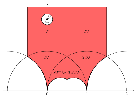
Figure 2: Fundamental domain $\mathcal{U}_{\varepsilon}$ for $\tau$: the fundamental domain $\mathbb{H}/\Gamma(2)$ with the $\varepsilon$-neighborhood of $\tau_{\rm uv}$, $B(\tau_{\rm uv},\varepsilon)$, excluded.

The integral $\Phi_{\boldsymbol{\mu}}^{J}$ now reads

$$\Phi_{\boldsymbol{\mu}}^{J}=\lim_{\varepsilon\to 0}\int_{\mathcal{U}_{\varepsilon}}d\tau\wedge d\bar{\tau}\,\nu(\tau,\tau_{\rm uv},m)\,\Psi^{J}_{\boldsymbol{\mu}}(\tau,\bar{\tau},v{\boldsymbol{k}}_{m},\bar{v}{\boldsymbol{k}}_{m}),$$ (183)

where we defined the measure $\nu$,

$$\nu(\tau,\tau_{\rm uv},m)=K_{u}\,\eta(\tau_{\rm uv})^{-4\ell-2\chi}\,\frac{da}{d\tau}\,A^{\chi}\,B^{\sigma}\,C^{{\boldsymbol{k}}_{m}^{2}}.$$ (184)

We express $\nu$ more explicitly using (35), (39), (42) and Matone’s relation [89] for $\mathcal{N}=2^{*}$ theory,

$$\frac{1}{2\pi i}\frac{du}{d\tau}=\frac{8}{m^{2}}\,\Delta_{\rm phys}\left(\frac{da}{du}\right)^{2}.$$ (185)

This gives,

$$\begin{split}\nu(\tau,\tau_{\rm uv},m)&=\frac{16\pi i\,K_{u}\,\alpha^{\chi}\,\beta^{\sigma}}{m^{2}}\,\eta(\tau_{\rm uv})^{-4\ell-2\chi}\,\left(\frac{du}{da}\right)^{\frac{\chi}{2}-3}\,\Delta_{\rm phys}^{\frac{\sigma}{8}+1}\,C^{{\boldsymbol{k}}_{m}^{2}}\\ &=\frac{\kappa\,m^{\frac{\sigma}{8}-2}}{4\,\eta(\tau_{\rm uv})^{2\chi+4\ell}}\left(\frac{4}{\Lambda}\right)^{\frac{3}{8}(2\chi+3\sigma)}\left(\frac{du}{da}\right)^{\frac{\chi}{2}-3}\,\Delta_{\rm phys}^{\frac{\sigma}{8}+1}\,C^{{\boldsymbol{k}}_{m}^{2}}.\end{split}$$ (186)

4.6 Single-valuedness of the $u$-plane integrand

In the following subsections, we discuss the single-valuedness of the integrand under monodromies around the four singularities of the Coulomb branch.

4.6.1 $\infty$

For the monodromy around $u=\infty$, we have $a\to e^{\pi i}a$ and $v\to e^{-\pi i}v$. The different ingredients of the integrand transform as follows:

$$\begin{split}&\frac{du}{da}\mapsto e^{\pi i}\,\frac{du}{da},\\ &\Delta_{\rm phys}\mapsto e^{6\pi i}\,\Delta_{\rm phys},\\ &C\mapsto e^{-\pi i}\,C.\end{split}$$ (187)

The sum over fluxes changes by a sign (175).

The integrand of $\Phi^{J}_{\boldsymbol{\mu}}$ therefore changes by a phase

$$e^{\pi i\,\chi/2+6\pi i\,\sigma/8-\pi i\,{\boldsymbol{k}}_{m}^{2}}.$$ (188)

For $b_{2}^{+}=1$, we have $\chi+\sigma=4$, such that this phase equals

$$e^{2\pi i\,\sigma/8-\pi i\,{\boldsymbol{k}}_{m}^{2}}.$$ (189)

Therefore, if we set ${\boldsymbol{k}}_{m}\in K/2+L$, with $K$ a characteristic vector of $L$ (78), then (189) equals 1. We thus find that ${\boldsymbol{k}}_{m}$ must correspond to a ${\rm Spin}^{c}$ structure, for the $u$-plane integral to be single-valued with respect to monodromies around $\infty$. We will demonstrate that this requirement also implies single-valuedness with respect to the monodromies around $u_{j}$, $j=1,2,3$.

4.6.2 $u_{1}$

For the monodromy around $u_{1}=\frac{m^{2}}{4}e_{1}$ (or $\tau\to i\infty$), we have using (48) and (56)

$$\begin{split}&\tau\mapsto\tau+2,\\ &v\mapsto v-1,\\ &\frac{du}{da}\mapsto\frac{du}{da},\\ &\Delta_{\rm phys}\mapsto e^{2\pi i}\,\Delta_{\rm phys},\\ &C\mapsto e^{-\pi i}C.\end{split}$$ (190)

For the sum over fluxes, we have using (179) and (176)

$$\begin{split}\Psi^{J}_{\boldsymbol{\mu}}(\tau+2,\bar{\tau}+2,{\boldsymbol{z}}-{\boldsymbol{k}}_{m},\bar{\boldsymbol{z}}-{\boldsymbol{k}}_{m})&=e^{2\pi iB({\boldsymbol{\mu}},K)}\,\Psi^{J}_{\boldsymbol{\mu}}(\tau,\bar{\tau},{\boldsymbol{z}}-{\boldsymbol{k}}_{m},\bar{\boldsymbol{z}}-{\boldsymbol{k}}_{m})\\ &=e^{2\pi iB({\boldsymbol{\mu}},K+2{\boldsymbol{k}}_{m})}\,\Psi^{J}_{\boldsymbol{\mu}}(\tau,\bar{\tau},{\boldsymbol{z}},\bar{\boldsymbol{z}}).\end{split}$$ (191)

The integrand is therefore multiplied by the following phase

$$e^{2\pi i\,\sigma/8-\pi i\,{\boldsymbol{k}}_{m}^{2}+2\pi iB({\boldsymbol{\mu}},K+2{\boldsymbol{k}}_{m})}.$$ (192)

Therefore for ${\boldsymbol{k}}_{m}\in K/2+L$, the integrand is single-valued for the monodromy around $u_{1}$. This condition on ${\boldsymbol{k}}_{m}$ is compatible with the condition found for the monodromy around $\infty$.

4.6.3 $u_{2}$

For the monodromy around $u_{2}=\frac{m^{2}}{4}e_{2}$, we have using (50) and (57)

$$\begin{split}&\tau\mapsto\frac{\tau}{-2\tau+1},\\ &v\mapsto\frac{v-\tau}{-2\tau+1},\\ &\frac{du}{da}\mapsto(-2\tau+1)^{-1}\,\frac{du}{da},\\ &\Delta_{\rm phys}\mapsto e^{2\pi i}\,\Delta_{\rm phys},\\ &C\mapsto e^{-\pi i+2\pi iv-2\pi i(v-\tau)(2v-1)/(-2\tau+1)}\,C.\end{split}$$ (193)

Finally we need to determine the transformation of $\Psi^{J}_{\boldsymbol{\mu}}$. We have

$$\begin{split}&\Psi^{J}_{\boldsymbol{\mu}}\!\left(\frac{\tau}{-2\tau+1},\frac{\bar{\tau}}{-2\bar{\tau}+1},\frac{v-\tau}{-2\tau+1}{\boldsymbol{k}}_{m},\frac{\bar{v}-\bar{\tau}}{-2\bar{\tau}+1}{\boldsymbol{k}}_{m}\right)\\ &=\exp\!\left(2\pi i\left(\frac{\tau\,{\boldsymbol{k}}_{m}^{2}-2\,v\,{\boldsymbol{k}}_{m}^{2}}{-2\tau+1}\right)\right)\,\Psi^{J}_{{\boldsymbol{\mu}}-{\boldsymbol{k}}_{m}}\!\left(\frac{\tau}{-2\tau+1},\frac{\bar{\tau}}{-2\bar{\tau}+1},\frac{v}{-2\tau+1}{\boldsymbol{k}}_{m},\frac{\bar{v}}{-2\bar{\tau}+1}{\boldsymbol{k}}_{m}\right)\\ &=(-2\tau+1)^{b_{2}/2}\,(-2\bar{\tau}+1)^{2}\,\exp\!\left(2\pi i\frac{(\tau-2\,v+2\,v^{2})\,{\boldsymbol{k}}_{m}^{2}}{-2\tau+1}\right)\\ &\quad\times\Psi^{J}_{{\boldsymbol{\mu}}-{\boldsymbol{k}}_{m}-K/2}\!\left(\tau,\bar{\tau},v\,{\boldsymbol{k}}_{m},\bar{v}\,{\boldsymbol{k}}_{m}\right),\end{split}$$ (194)

where we used (176) for the first equality sign, and (179) for the second.

The weights of the various functions and $d\tau\wedge d\bar{\tau}$ cancel among each other. Moreover, the terms involving $v$ cancel beautifully between $C^{{\boldsymbol{k}}_{m}^{2}}$ and $\Psi^{J}_{\boldsymbol{\mu}}$. The remaining phase is

$$e^{2\pi i\sigma/8-\pi i{\boldsymbol{k}}_{m}^{2}}$$ (195)

which evaluates to $1$ for ${\boldsymbol{k}}_{m}\in K/2+L$. Finally, for this choice of ${\boldsymbol{k}}_{m}$, $\Psi_{{\boldsymbol{\mu}}-{\boldsymbol{k}}_{m}-K/2}^{J}=\Psi_{{\boldsymbol{\mu}}}^{J}$. We thus conclude that the integrand is single-valued under the monodromy around $u_{2}$ if ${\boldsymbol{k}}_{m}$ represents a ${\rm Spin}^{c}$ structure.

4.6.4 $u_{3}$

This monodromy must be single-valued too, since $M_{1}\,M_{2}\,M_{3}=M_{\infty}$. As a check, we determine the various transformations using (LABEL:aDaz3) and (58)

$$\begin{split}&\tau\mapsto\frac{-\tau+2}{-2\tau+3},\\ &v\mapsto\frac{v-\tau+1}{-2\tau+3},\\ &\frac{du}{da}\mapsto(-2\tau+3)^{-1}\,\frac{du}{da},\\ &\Delta_{\rm phys}\mapsto e^{2\pi i}\,\Delta_{\rm phys},\\ &C\mapsto e^{-\pi i-2\pi i(\tau-1-2v+v^{2})/(-2\tau+3)}C.\end{split}$$ (196)

4.7 The limit to $N_{f}=0$

Note the sum over fluxes $\Psi_{\boldsymbol{\mu}}^{J}(\tau,\bar{\tau},v{\boldsymbol{k}}_{m},\bar{v}{\boldsymbol{k}}_{m})$ appears at first sight to differ from the theory with $N_{f}=0$, since there is no insertion $(-1)^{B({\boldsymbol{k}},K)}$. However, (197) demonstrates that this will appear in the limit.

The non-perturbative contributions to $v$ and $\xi$ vanish in the limit to the pure SW theory. Equation (25) shows that their perturbative parts evaluates to constants. From (60), one obtains for the three couplings

$$\tau\mapsto\tau,\qquad v=-\frac{1}{2}+O(q_{\rm uv}),\qquad\xi\mapsto-\frac{1}{4}-\frac{1}{2\pi i}\frac{3}{2}\log(\Lambda/m)+O(q_{\rm uv}),$$ (197)

One of the striking effects of this limit is that the non-holomorphic, non-topological coupling

$$e^{-4\pi ivB({\boldsymbol{k}}_{-},{\boldsymbol{k}}_{m})-4\pi i\bar{v}B({\boldsymbol{k}}_{+},{\boldsymbol{k}}_{m})}$$ (198)

in (171) and (180), becomes holomorphic and topological,

$$e^{-2\pi iB({\boldsymbol{k}}_{m},{\boldsymbol{k}})}.$$ (199)

This phase is crucial in the sum over fluxes of the effective theory of pure SW theory.

The topological couplings for the $N_{f}=0$ theory, $A_{0}$ and $B_{0}$ are defined as in (35), with for $\alpha_{0}$ and $\beta_{0}$ [49]

$$\alpha_{0}=\Lambda^{-1/2},\qquad\beta_{0}=\sqrt{2}\,\Lambda^{-1/2}.$$ (200)

From (35) and (39), we deduce that in the limit to pure $SU(2)$ the gravitational couplings $A$, $B$ and $C$ become

$$A\to A_{0},\qquad B\to\left(\frac{m}{\Lambda}\right)^{3/8}e^{-\pi i/8}B_{0},\qquad C\to\left(\frac{\Lambda}{m}\right)^{3/2}e^{\pi i/2}.$$ (201)

The measure $\nu_{0}(\tau)$ of the $u$-plane integral for pure SW-theory is

$$\nu_{0}(\tau)=-\frac{i}{4}\frac{\vartheta_{4}(2\tau)^{13-b_{2}}}{\eta(2\tau)^{9}},$$ (202)

while the sum over fluxes reads

$$\Psi^{J}_{0,{\boldsymbol{\mu}}}(\tau,\bar{\tau})=\sum_{{\boldsymbol{k}}\in L+{\boldsymbol{\mu}}}\partial_{\bar{\tau}}\left(\sqrt{4y}B({\boldsymbol{k}},J)\right)e^{\pi iB({\boldsymbol{k}},K_{0})}q^{-{\boldsymbol{k}}_{-}^{2}}\bar{q}^{{\boldsymbol{k}}_{+}^{2}},$$ (203)

with $K_{0}$ a characteristic vector of $L$, and therefore $K_{0}\in\bar{w}_{2}(X)+2L$. Two different choices for the characteristic vector, $K_{0}$ and $\tilde{K}_{0}$, change $\Psi^{J}_{0,{\boldsymbol{\mu}}}$ by a sign, $(-1)^{B({\boldsymbol{\mu}},K_{0}-\tilde{K}_{0})}$. This dependence on the lift of $w_{2}(X)$, can be compensated by an additional sign in $\Psi^{J}_{0,{\boldsymbol{\mu}}}$ [5],

$$e^{\frac{i\pi}{2}((2{\boldsymbol{\mu}})^{2}-B(2{\boldsymbol{\mu}},K_{0}))},$$ (204)

with $2{\boldsymbol{\mu}}$ a lift of $w_{2}(E)$ to $L$ as before. With (204), $\Psi^{J}_{0,{\boldsymbol{\mu}}}$ is independent of $K_{0}$, and the change of sign, due to a different choice of ${\boldsymbol{\mu}}$, corresponds to a change of orientation of instanton moduli space discussed in [62, Section 7.1.6].

The $N_{f}=0$ limit of $\nu$ is

$$\nu(\tau,\tau_{\rm uv},m)\sim i\,\kappa\,\eta(\tau_{\rm uv})^{-4\ell-2\chi}\left(\frac{\Lambda}{m}\right)^{\frac{3}{2}({\boldsymbol{k}}_{m}^{2}-\frac{\sigma}{4})}\,e^{\pi i({\boldsymbol{k}}_{m}^{2}/2-\sigma/8)}\,\nu_{0}(\tau).$$ (205)

Moreover, the $N_{f}=0$ limit of the $\mathcal{N}=2^{*}$ sum over fluxes is

$$\Psi^{J}_{{\boldsymbol{\mu}}}(\tau,\bar{\tau},v{\boldsymbol{k}}_{m},\bar{v}{\boldsymbol{k}}_{m})\to(-1)^{B({\boldsymbol{\mu}},K_{0}-2{\boldsymbol{k}}_{m})}\,\Psi^{J}_{0,{\boldsymbol{\mu}}}(\tau,\bar{\tau}).$$ (206)

Put differently, the $N_{f}=0$ limit leads to a canonical choice of $K_{0}=2{\boldsymbol{k}}_{m}=c_{\rm uv}$. Combining the factors, we find that for the $N_{f}=0$ limit, $\Phi_{\boldsymbol{\mu}}^{J}$ and $Z_{\boldsymbol{\mu}}$ more generally, should be multiplied by

$$R_{\boldsymbol{\mu}}^{X}(K_{0},2{\boldsymbol{k}}_{m})=e^{-\pi i(\chi+\sigma)/8}\,(-1)^{B({\boldsymbol{\mu}},K_{0}-2{\boldsymbol{k}}_{m})+({\boldsymbol{k}}_{m}^{2}/2-\sigma/8)}\,\eta(\tau_{\rm uv})^{2\chi+4\ell}\times\left(\frac{m}{\Lambda}\right)^{\frac{3}{2}({\boldsymbol{k}}_{m}^{2}-\frac{\sigma}{4})},$$ (207)

where we have replaced $-i$ by $e^{-\pi i(\chi+\sigma)/8}$, such that this formula can be applied to study this limit for generic manifolds of simple type in Section 7.5. We have also set $\kappa=1$, which will follow from explicit calculation in Section 6.2.

For later reference, we define the dimensionless partition function $\underline{\Phi}_{\boldsymbol{\mu}}^{J}$,

$$\underline{\Phi}_{\boldsymbol{\mu}}^{J}(\tau_{\rm uv},\bar{\tau}_{\rm uv})=R_{\boldsymbol{\mu}}^{X}(K_{0},2{\boldsymbol{k}}_{m})\,\Phi_{\boldsymbol{\mu}}^{J}(\tau_{\rm uv},\bar{\tau}_{\rm uv}).$$ (208)

The leading term of $\underline{\Phi}_{\boldsymbol{\mu}}^{J}$ is a constant $\sim q_{\rm uv}^{0}$, since 0 is the smallest instanton number.

4.8 Observables

The $\mathcal{N}=2^{*}$ theory gives rise to correlation functions of non-trivial observables. The observables are proportional to the mass $m$, and vanish in the massless limit.

The point observable
It is straightforward to include the point observable, which corresponds to the order parameter $u$ on the Coulomb branch. Mathematically, this observable corresponds to a 4-form $\mu_{D}(p)$ on the instanton moduli space, where $\mu_{D}:H_{i}(X,\mathbb{Q})\to H^{4-i}(\mathcal{M}_{k,{\boldsymbol{\mu}}},\mathbb{Q})$ is Donaldson’s $\mu$-map. Since the limit to pure SW theory (197) involves a shift, the appropriate $\mathcal{N}=2^{*}$ observable is

$$u_{\rm D}=u+\frac{1}{8}e_{1}(\tau_{\rm uv})m^{2}.$$ (209)

We determine the normalization by the limit to the pure theory.

$$e^{pu_{\rm D}/\Lambda^{2}}.$$ (210)

If $u$ approaches the singularities $u_{j}$, $j=1,2,3$, $u_{\rm D}(\tau,\tau_{\rm uv})$ approaches

$$\begin{split}u_{{\rm D},1}&=\tfrac{3}{8}m^{2}e_{1}(\tau_{\rm uv})=m^{2}\left(\tfrac{1}{4}+6\,q_{\rm uv}+O(q_{\rm uv}^{2})\right),\\ u_{{\rm D},2}&=\tfrac{1}{4}m^{2}e_{2}(\tau_{\rm uv})+\tfrac{1}{8}m^{2}e_{1}(\tau_{\rm uv})=-2\,m^{2}\,q_{\rm uv}^{1/2}+O(q_{\rm uv})\\ &=\Lambda_{0}^{2}\,(1+O(q_{\rm uv}^{1/2})),\\ u_{{\rm D},3}&=\tfrac{1}{4}m^{2}e_{3}(\tau_{\rm uv})+\tfrac{1}{8}m^{2}e_{1}(\tau_{\rm uv})=2\,m^{2}\,q_{\rm uv}^{1/2}+O(q_{\rm uv})\\ &=-\Lambda_{0}^{2}\,(1+O(q_{\rm uv}^{1/2})).\\ \end{split}$$ (211)

Thus $u_{{\rm D},1}$ diverges in the limit to pure SW, while $u_{{\rm D},2}$ and $u_{{\rm D},3}$ approach the strong coupling singularities of the pure theory.

The surface observable
For $S\in H_{2}(X,\mathbb{Q})$, the surface observable reads

$$I_{-}(S)=\frac{1}{4\pi^{2}}\int_{S}{\rm Tr}\left[\frac{1}{8}\psi\wedge\psi-\frac{1}{\sqrt{2}}\phi F\right].$$ (212)

The coupling flows in the infra-red to:

$$\tilde{I}_{-}(S)=\frac{i}{\sqrt{2}\pi}\int_{S}\left(\frac{1}{32}\frac{d^{2}u}{da^{2}}\psi\wedge\psi-\frac{\sqrt{2}}{4}\frac{du}{da}(F_{-}+D)\right).$$ (213)

Then we add to the effective action

$$e^{\tilde{I}_{-}(S)/\Lambda}.$$ (214)

The overall normalization is such that the leading power of $q$ of the Seiberg-Witten limit (197) of $\tilde{I}_{-}$ is $q^{-1/4}B(S,F/4\pi)=q^{-1/4}B(S,{\boldsymbol{k}}_{m})$.

After reduction to zero modes and integrating over $D$, the insertion of the surface operator $e^{\tilde{I}_{-}(S)}$ in the effective action is taken into account by adding an extra term to $v{\boldsymbol{k}}_{m}$ in (180),

$${\boldsymbol{z}}_{S}=\frac{S}{4\pi\,\Lambda}\frac{du}{da},\qquad v{\boldsymbol{k}}_{m}\mapsto v{\boldsymbol{k}}_{m}+{\boldsymbol{z}}_{S},\qquad\bar{v}{\boldsymbol{k}}_{m}\mapsto\bar{v}{\boldsymbol{k}}_{m},$$ (215)

In this way, we can easily take the surface observable into account in the sum over fluxes. This becomes

$$\Psi_{\boldsymbol{\mu}}^{J}(\tau,\bar{\tau},v{\boldsymbol{k}}_{m}+{\boldsymbol{z}}_{S},\bar{v}{\boldsymbol{k}}_{m}),$$ (216)

with $\Psi_{\boldsymbol{\mu}}^{J}$ as in (171). For the monodromy $M_{2}$, (194) is modified to

$$\begin{split}&\Psi^{J}_{\boldsymbol{\mu}}\!\left(\frac{\tau}{-2\tau+1},\frac{\bar{\tau}}{-2\bar{\tau}+1},\frac{(v-\tau){\boldsymbol{k}}_{m}+{\boldsymbol{z}}_{S}}{-2\tau+1},\frac{(\bar{v}-\bar{\tau}){\boldsymbol{k}}_{m}}{-2\bar{\tau}+1}\right)\\ &=\exp\!\left(2\pi i\frac{(\tau-2\,v+2\,v^{2})\,{\boldsymbol{k}}_{m}^{2}+(4v-2)B({\boldsymbol{k}}_{m},{\boldsymbol{z}}_{S})+2{\boldsymbol{z}}_{S}^{2}}{-2\tau+1}\right)\\ &\quad\times(-2\tau+1)^{b_{2}/2}\,(-2\bar{\tau}+1)^{2}\,\Psi^{J}_{{\boldsymbol{\mu}}}\!\left(\tau,\bar{\tau},v\,{\boldsymbol{k}}_{m}+{\boldsymbol{z}}_{S},\bar{v}\,{\boldsymbol{k}}_{m}\right).\end{split}$$ (217)

Contact term $T_{2}$
Since ${\boldsymbol{z}}_{S}\sim S$ appears in the exponential prefactor, we deduce that single valuedness of the integrand requires the presence of contact terms in the effective action [8, 5, 87]. We denote the term for $S^{2}$ is by $e^{T_{2}\,S^{2}}$, and for $B({\boldsymbol{k}}_{m},{\boldsymbol{z}})$ by $e^{T_{3}\,B({\boldsymbol{k}}_{m},{\boldsymbol{z}})}$. We discuss first $T_{2}$, which is given by

$$T_{2}(\tau,\tau_{\rm uv})=\frac{1}{2\pi i\Lambda^{2}}\frac{\partial^{2}\widetilde{\mathcal{F}}(a,m,\tau_{\rm uv})}{\partial\tau_{\rm uv}^{2}},$$ (218)

where the derivative to $\tau_{\rm uv}$ is for fixed $a$ and $m$. We can express this function in terms of $u$ and $du/da$ [92],

$$\begin{split}T_{2}(\tau,\tau_{\rm uv})&=\frac{1}{24\Lambda^{2}}\left(-\frac{E_{2}(\tau)}{2}\left(\frac{du}{da}\right)^{2}+2\,E_{2}(\tau_{\rm uv})\,u+\frac{m^{2}}{6}E_{4}(\tau_{\rm uv})+\frac{m^{2}}{\pi i}\,\frac{dE_{2}(\tau_{\rm uv})}{d\tau_{\rm uv}}\right)\\ &=\frac{1}{24\Lambda^{2}}\left(-\frac{E_{2}(\tau)}{2}\left(\frac{du}{da}\right)^{2}+2\,E_{2}(\tau_{\rm uv})\,u+\frac{m^{2}}{6}\,E_{2}(\tau_{\rm uv})^{2}\,\right),\end{split}$$ (219)

where we used (530) for the second identity.

We can derive the modular properties also from (218). Using (43), we can write $T_{2}$ as a derivative of $u$,

$$\frac{\partial^{2}\widetilde{\mathcal{F}}(a,m,\tau_{\rm uv})}{\partial\tau_{\rm uv}^{2}}=\left.\frac{\partial}{\partial\tau_{\rm uv}}\left(\tfrac{1}{2}u+\tfrac{m^{2}}{12}E_{2}(\tau_{\rm uv})\right)\right|_{a,m},$$ (220)

where we consider $u$ as a function of $a$, $m$ and $\tau_{\rm uv}$. We next change variables from $a$ to $\tau$ for $u$, such that $\partial^{2}_{\tau_{\rm uv}}\widetilde{\mathcal{F}}$ becomes

$$\begin{split}\frac{\partial\widetilde{\mathcal{F}}(a,m,\tau_{\rm uv})}{\partial\tau_{\rm uv}^{2}}=&\left.\frac{\partial}{\partial\tau_{\rm uv}}\left(\tfrac{1}{2}u(\tau,\tau_{\rm uv},m)+\tfrac{m^{2}}{12}E_{2}(\tau_{\rm uv})\right)\right|_{\tau,m}\\ &+\frac{1}{2}\left.\frac{\partial u(\tau,\tau_{\rm uv},m)}{\partial\tau}\right|_{\tau_{\rm uv},m}\,\left.\frac{\partial\tau(a,\tau_{\rm uv},m)}{\partial\tau_{\rm uv}}\right|_{a,m}.\end{split}$$ (221)

Using that the last term equals $\partial\tau/\partial\tau_{\rm uv}=\frac{1}{2}\partial^{2}u/\partial a^{2}$, we can determine the transformations as in Section 2.7. This gives

$$M_{2}:\qquad\frac{\partial^{2}\widetilde{\mathcal{F}}}{\partial\tau_{\rm uv}^{2}}\mapsto\frac{\partial^{2}\widetilde{\mathcal{F}}}{\partial\tau_{\rm uv}^{2}}+\frac{1}{2(-2\tau+1)}\left(\frac{du}{da}\right)^{2},$$ (222)

where we used $\partial_{a}\mapsto 1/(-2\tau+1)\partial_{a}$ (50).

We have moreover for $SL(2,\mathbb{Z})$ transformations of $\tau_{\rm uv}$,

$$\begin{split}T_{2}\!\left(\tau,\frac{a\tau_{\rm uv}+b}{c\tau_{\rm uv}+d}\right)&=(c\tau_{\rm uv}+d)^{4}\,\left(T_{2}(\tau,\tau_{\rm uv})+\frac{1}{2\pi i\,\Lambda^{2}}\frac{c}{c\tau_{\rm uv}+d}\,\left(u+\frac{m^{2}}{6}E_{2}(\tau_{\rm uv})\right)\right.\\ &\qquad\left.-\frac{m^{2}}{4}\frac{c^{2}}{(c\tau_{\rm uv}+d)^{2}}\right).\end{split}$$ (223)

where we used (30).

The last aspect we mention here is the limit of $T_{2}$ to the $N_{f}=0$ theory. Denoting this limit by $T_{2,0}$, we find

$$T_{2,0}(\tau)=\frac{1}{24\Lambda_{0}^{2}}\left(u_{0}-E_{2}(\tau)\left(\frac{du}{da}\right)^{2}_{0}\right),$$

where $u_{0}$ is as in Equation (12).

Contact term $T_{3}$
Due to the coupling $B({\boldsymbol{k}}_{m},{\boldsymbol{z}})$, there must be a third contact term. We will demonstrate that this contact term is given by

$$T_{3}(\tau,\tau_{\rm uv})=-\frac{2i}{\Lambda}\frac{\partial^{2}\widetilde{\mathcal{F}}}{\partial\tau_{\rm uv}\partial m},$$ (224)

where the derivatives act for fixed $a$. Again using (30), we can write $T_{3}$ as a derivative of $u$ to $m$ for fixed $a$. Changing variables from $a$ to $\tau$, we can express $\partial^{2}\widetilde{\mathcal{F}}/\partial\tau_{\rm uv}\partial m$ as

$$\frac{\partial^{2}\widetilde{\mathcal{F}}(a,m,\tau_{\rm uv})}{\partial\tau_{\rm uv}\partial m}=\tfrac{1}{2}\partial_{m}(u+\tfrac{m^{2}}{6}E_{2}(\tau_{\rm uv}))|_{\tau,\tau_{\rm uv}}+\tfrac{1}{2}\partial_{\tau}u|_{\tau_{\rm uv},m}\,\partial_{m}\tau|_{a,\tau_{\rm uv}}$$ (225)

Using that $\partial_{m}\tau=\partial^{2}m_{D}/\partial a^{2}$, we can use the transformations of $m_{D}$ and $a$ to derive the transformations of $T_{3}$. We then find using $v=\partial_{a}m_{D}$,

$$\begin{split}&M_{\infty},M_{1}:\qquad\frac{\partial^{2}\widetilde{\mathcal{F}}}{\partial\tau_{\rm uv}\partial m}\mapsto\frac{\partial^{2}\widetilde{\mathcal{F}}}{\partial\tau_{\rm uv}\partial m},\\ &M_{2}\qquad\,:\qquad\frac{\partial^{2}\widetilde{\mathcal{F}}}{\partial\tau_{\rm uv}\partial m}\mapsto\frac{\partial^{2}\widetilde{\mathcal{F}}}{\partial\tau_{\rm uv}\partial m}+\frac{2v-1}{2(-2\tau+1)}\frac{du}{da}.\end{split}$$ (226)

These transformations are of the expected form to match the transformation of the sum over fluxes (217).

To write $T_{3}$ more explicitly, we use

$$\left.\frac{\partial\tau}{\partial m}\right|_{a,\tau_{\rm uv}}=-\frac{a}{m}\left.\frac{\partial\tau}{\partial a}\right|_{m,\tau_{\rm uv}}.$$ (227)

Moreover, we determine from (32) that

$$a=-m\frac{dv}{d\tau}.$$ (228)

We then arrive at

$$T_{3}(\tau,\tau_{\rm uv})=-\frac{2i}{\Lambda}\left(\frac{u}{m}+\frac{m}{6}\,E_{2}(\tau_{\rm uv})+\frac{1}{2}\frac{dv}{d\tau}\,\frac{du}{da}\right).$$ (229)

Therefore, under an $SL(2,\mathbb{Z})$ transformation of $\tau_{\rm uv}$, we have

$$T_{3}\!\left(\tau,\frac{a\tau_{\rm uv}+b}{c\tau_{\rm uv}+d}\right)=(c\tau_{\rm uv}+d)^{2}\left(T_{3}(\tau,\tau_{\rm uv})-\frac{2m}{\pi\Lambda}\frac{c}{c\tau_{\rm uv}+d}\right).$$ (230)

Finally, we consider the $N_{f}=0$ limit. This limit of $T_{3,0}$ in fact diverges,

$$\lim_{\mathcal{N}=2^{*}\to N_{f}=0}T_{3}=\infty.$$ (231)

On the other hand, the limit of $\partial^{2}\mathcal{F}/\partial\tau_{\rm uv}\partial m$ vanishes. Since the $N_{f}=0$ limit of $T_{3}$ is infinite, we define an alternative contact term by replacing $u$ with $u_{\rm D}$ (209) in (229), and subtract the term involving $E_{2}$. We have then

$$T_{{\rm D},3}=T_{3}+\frac{i\,m}{3\Lambda}E_{2}(\tau_{\rm uv})-\frac{i\,m}{4\Lambda}e_{1}(\tau_{\rm uv}).$$ (232)

4.9 Regularization of the $u$-plane integral

The $u$-plane integrand often diverges near the singularities, which will become more clear from the discussion in Section 5.1. Due to the divergences, it is necessary to reguralize the integral. To this end, we first compactify $\mathcal{U}_{\varepsilon}$ by introducing a cut-off $\mathrm{Im}(\tau)\leq Y$ for the cusp $\tau=\tau_{1}\to i\infty$, and similarly for the local couplings $\tau_{2}$ and $\tau_{3}$ near the cusps $\tau=0$ and $\tau=1$. We denote this space by $\mathcal{U}_{Y,\varepsilon}$. Then $\Phi_{\boldsymbol{\mu}}^{J}$ is defined as

$$\begin{split}\Phi_{\boldsymbol{\mu}}^{J}&=\lim_{Y\to\infty,\varepsilon\to 0}K_{u}\,\eta(\tau_{\rm uv})^{-4\ell-2\chi}\,\alpha^{\chi}\beta^{\sigma}\\ &\qquad\times\int_{\mathcal{U}_{Y,\varepsilon}}d\tau\wedge d\bar{\tau}\,\left(\frac{du}{da}\right)^{\frac{\chi}{2}-1}\frac{du}{d\tau}\,\Delta_{\rm phys}^{\frac{\sigma}{8}}\,C^{{\boldsymbol{k}}_{m}^{2}}\,\Psi^{J}_{\boldsymbol{\mu}}(\tau,\bar{\tau},v{\boldsymbol{k}}_{m},\bar{v}{\boldsymbol{k}}_{m}),\end{split}$$ (233)

assuming that the limits exist. This integral requires careful regularization, especially if observables are included. We will assume that the $\tau$-dependent of the integrand is a linear combination of the following terms near the boundaries $u_{j}$ and $\infty$,

$$\begin{split}&\text{For}\,\,u\to u_{j}:\qquad y^{s}q_{j}^{m}\bar{q}_{j}^{n},\qquad n\geq 0,m-n\in\mathbb{Z}/2,\\ &\text{For}\,\,u\to\infty:\qquad(\tau-\tau_{\rm uv})^{m}(\bar{\tau}-\bar{\tau}_{\rm uv})^{n},\qquad n\geq 0,m-n\in\mathbb{Z}.\end{split}$$ (234)

where $q_{j}=e^{2\pi i\tau_{j}}$ with $\tau_{1}=\tau$, $\tau_{2}=-1/\tau$ and $\tau_{3}=-1/(\tau-1)$. The analysis in Section 5 will confirm that the expansions of the $u$-plane integrand are of the form in (234). For the cusps $u_{j}$, the ”familiar” regularization is then applicable [93, 94, 95]. For example for $u_{1}$, we have

$$\int^{Y}_{Y_{0}}dy\int_{-1/2}^{3/2}dx\,y^{s}q_{j}^{m}\bar{q}_{j}^{n}=2\delta_{m,n}\int^{Y}_{Y_{0}}y^{s}e^{-4\pi ym},$$ (235)

which is convergent for $Y\to\infty$ for $n>0$, and for $s<-1$ if $n=0$. Similarly for $u\to\infty$, we have

$$\int^{r_{0}}_{\varepsilon}r\,dr\int_{0}^{2\pi}d\varphi\,(\tau-\tau_{\rm uv})^{m}(\bar{\tau}-\bar{\tau}_{\rm uv})^{n}=2\pi\delta_{m,n}\int^{r_{0}}_{\varepsilon}dr\,r^{2m+1},$$ (236)

with $\tau-\tau_{\rm uv}=r\,e^{i\varphi}$. This is also convergent for $\varepsilon\to 0$ for $n\geq 0$. With this regularization, we thus have a well-defined $u$-plane integral.

It is possible to introduce observables to the path integral, which violate the condition $n\geq 0$ in Equation (234) and which are therefore not included in Section 4.8. An example is the anti-holomorphic surface observable [96, 24]

$$\tilde{I}_{+}(S)=-\frac{i}{\sqrt{2}\pi}\int_{S}\frac{1}{2}\frac{d^{2}\bar{u}}{d\bar{a}^{2}}\eta\chi+\frac{\sqrt{2}}{4}\frac{d\bar{u}}{d\bar{a}}(F_{+}-D)$$

Such observables lead to a more severe divergence than the divergences occuring if (234) is satisfied. We therefore had to make the non-symmetric replacement of $v{\boldsymbol{k}}_{m}$ and $\bar{v}{\boldsymbol{k}}_{m}$ in (215). For the $N_{f}=0$ theory, such severe divergences were regularized in [97]. This regularization also applies to the cusps $u_{1}$, $u_{2}$ and $u_{3}$ of the $\mathcal{N}=2^{*}$ theory. We expect that such divergences for $u\to\infty$ can be treated in a similar way, but will leave this for future work.

4.10 Evaluation using Stokes’ Theorem

Having established the regularization of the integral, we proceed with outlining the evaluation using Stokes’ Theorem, which follows [96, 88, 24]. The $u$-plane integral $\Phi_{\boldsymbol{\mu}}^{J}$ is schematically of the form

$$\Phi^{J}_{\boldsymbol{\mu}}=\int_{\mathcal{B}}\omega.$$ (237)

We aim to express $\omega$ manifestly as an exact form, $\omega=d\Omega$, with $\Omega$ being a smooth 1-form on $\mathcal{B}$. We can then evaluate $\Phi^{J}_{\boldsymbol{\mu}}$ on the boundary $\partial\mathcal{B}$

$$\Phi^{J}_{\boldsymbol{\mu}}=\int_{\partial\mathcal{B}}\Omega.$$ (238)

There is an ambiguity in the choice of $\Omega$, since for a closed one-form $\varphi$, replacing $\Omega$ by $\Omega+\varphi$ does not change the integral. This is simply a choice of integration constant. $\varphi$ can be written as a linear combination of closed, non-exact one-forms. Since the Coulomb branch of the $\mathcal{N}=2^{*}$ is a four punctured sphere, it has three independent one-cycles, and consequently three independent closed, non-exact one-forms $\varphi_{j}$, $j=1,2,3$. One can choose the following representatives

$$\begin{split}\varphi_{1}&=\vartheta_{3}(\tau)^{4}\,d\tau,\\ \varphi_{2}&=\vartheta_{4}(\tau)^{4}\,d\tau,\\ \varphi_{3}&=\frac{\vartheta_{3}(\tau)^{4}\,\vartheta_{4}(\tau)^{4}}{\vartheta_{3}(\tau)^{4}\,\vartheta_{4}(\tau_{\rm uv})^{4}-\vartheta_{4}(\tau)^{4}\,\vartheta_{3}(\tau_{\rm uv})^{4}}\,d\tau.\end{split}$$ (239)

The integrals of $\varphi_{j}$ along the boundary arcs in $\partial\mathcal{B}$ vanish. The integral of $\varphi_{1}$ receives two non-vanishing, opposite contributions from arcs around $u_{1}$ and $u_{2}$. Similarly, the non-vanishing contributions for $\varphi_{2}$ are due to $u_{1}$ and $u_{3}$, and for $\varphi_{3}$ due to $u_{\infty}$ and $u_{1}$. Using the ambiguity in $\Omega$, one can in principle “fix” the contribution from three out of four cusps. On the other hand, we can require that the magnitude of the anti-derivative near each of the boundaries of $\mathcal{B}$ is of the same order as that of the integrand. This fixes the anti-derivative uniquely, and appears to be the most natural choice from the physical perspective.

Concretely, (183) demonstrates that $\omega$ reads

$$d\tau\wedge d\bar{\tau}\,\nu\,\Psi_{\boldsymbol{\mu}}^{J}.$$ (240)

To express the integrand as an exact form, we write the integrand $\nu\,\Psi_{\boldsymbol{\mu}}^{J}$ as a total deriviative using mock modular forms,

$$\nu(\tau,\tau_{\rm uv},m)\,\Psi_{\boldsymbol{\mu}}^{J}(\tau,\bar{\tau},v{\boldsymbol{k}}_{m},\bar{v}{\boldsymbol{k}}_{m})=\frac{d}{d\bar{\tau}}\widehat{\mathcal{H}}_{\boldsymbol{\mu}}^{J}(\tau,\bar{\tau},\tau_{\rm uv},m).$$ (241)

The 1-form $\Omega$ from (238) then reads

$$\Omega=-d\tau\,\widehat{\mathcal{H}}_{\boldsymbol{\mu}}^{J}(\tau,\bar{\tau},\tau_{\rm uv},m),$$ (242)

and the orientation of $\partial\mathcal{B}$ is such that “the interior of $\mathcal{B}$ is on the lhs”. The integral can now be written as a sum of contributions from the various boundary components of the Coulomb branch. For $\mathcal{N}=2^{*}$, the boundaries are a circle of radius $\varepsilon$ around $\tau=\tau_{\rm uv}$, and the three arcs around the cusps of $\mathbb{H}/\Gamma(2)$, which we take at $\tau=0,2$ and $i\infty$. Reversing the orientation of $\partial\mathcal{B}$, (183) is expressed as

$$\begin{split}\Phi_{\boldsymbol{\mu}}^{J}&=2[\widehat{\mathcal{H}}_{\boldsymbol{\mu}}^{J}(\tau,\bar{\tau},\tau_{\rm uv},m)]_{q^{0}}+2[\tau\mapsto-1/\tau]_{q^{0}}+2[\tau\mapsto 1-1/\tau]_{q^{0}}\\ &\quad+\lim_{\varepsilon\to 0}\oint_{|\tau-\tau_{\rm uv}|=\varepsilon}d\tau\,\widehat{\mathcal{H}}_{\boldsymbol{\mu}}^{J}(\tau,\bar{\tau},\tau_{\rm uv},m),\end{split}$$ (243)

with $\tau$ circling counter-clockwise around an $\varepsilon$-disc centered at $\tau_{\rm uv}$.

5 Analysis of the $u$-plane integral

This section will analyze the $u$-plane integral. We start with determining the behavior of various quantities near the singularities in Section 5.1, followed by derivations of $S$-duality, holomorphic anomaly, metric dependence and the effect of blowing-up a point on $X$ on $\Phi_{\boldsymbol{\mu}}^{J}$.

5.1 Behavior near the boundaries

Since the $u$-plane integral can be expressed as a sum of boundary contributions, it is important to analyze the behavior of the couplings $A$, $B$, $C$, $v$ and other quantities near the boundaries.

5.1.1 $u\to\infty$

We first consider the limit $u\to\infty$ or $\tau\to\tau_{\rm uv}$. To avoid ambiguities with the phases of square roots, we assume that $\mathrm{Im}(\tau-\tau_{\rm uv})>0$ and $\mathrm{Re}(\tau-\tau_{\rm uv})=0$.

The first terms for large $a$ are

$$\begin{split}&\frac{da}{du}=\frac{1}{2a}+O(a^{-5}),\\ &u=a^{2}-\frac{m^{2}}{12}E_{2}(\tau_{\rm uv})+O(a^{-2}),\\ &\Delta_{\rm phys}=a^{6}-\frac{m^{2}}{4}E_{2}(\tau_{\rm uv})\,a^{4}+O(a^{2}),\\ &v=\frac{1}{2\pi i}\left(\frac{m}{a}+\frac{m^{3}}{12a^{3}}E_{2}(\tau_{\rm uv})+O(a^{-5})\right),\\ &C=\left(\frac{\Lambda}{m}\right)^{3/2}\,\left(\frac{m}{2a}+\frac{m^{3}}{16a^{3}}E_{2}(\tau_{\rm uv})+O(a^{-5})\right).\\ \end{split}$$ (244)

Substitution of (34), with $s=-\pi i(\tau-\tau_{\rm uv})$, gives for the different ingredients of the $u$-plane integrand

$$\begin{split}&\frac{da}{du}=\frac{1}{m}\,s^{1/2}\left(1-\frac{E_{2}(\tau_{\rm uv})}{4}\,s+O(s^{2})\right),\\ &u=\frac{m^{2}}{4}s^{-1}+\frac{m^{2}}{24}E_{2}(\tau_{\rm uv})+O(s),\\ &\Delta_{\rm phys}=\left(\frac{m}{2}\right)^{6}s^{-3}\left(1+\frac{E_{2}(\tau_{\rm uv})}{2}\,s+O(s^{2})\right),\\ &v=\frac{1}{\pi i}\,s^{1/2}\left(1+\frac{E_{2}(\tau_{\rm uv})}{12}\,s+O\!\left(s^{2}\right)\right),\\ &C=\left(\frac{\Lambda}{m}\right)^{3/2}s^{1/2}\left(1+\frac{E_{2}(\tau_{\rm uv})}{4}\,s+O(s^{2})\right).\\ \end{split}$$ (245)

With these expansions, we are able to make a verification of the selection rule (151). We find for the behavior of the measure

$$\begin{split}\nu(\tau,\tau_{\rm uv},m)&=\frac{\kappa}{4\,\eta(\tau_{\rm uv})^{2\chi+4\ell}}\left(\frac{\Lambda}{m}\right)^{3\ell}s^{\ell-\frac{3}{2}}\left(1+N(c_{\rm uv})\,E_{2}(\tau_{\rm uv})\,s+O(s^{2})\right),\end{split}$$ (246)

where we used $\chi+\sigma=4$, and defined

$$\begin{split}\ell&=\frac{{\boldsymbol{k}}_{m}^{2}}{2}-\frac{(2\chi+3\sigma)}{8}\in\mathbb{Z}\\ N(c_{\rm uv})&=\frac{1}{4}\left(\frac{\chi}{2}-3\right)+\frac{1}{2}\left(\frac{\sigma}{8}+1\right)+\frac{{\boldsymbol{k}}_{m}^{2}}{4}\\ &=\frac{1}{16}(4-\sigma+c_{\rm uv}^{2}).\end{split}$$ (247)

For four-manifolds with $b_{2}=b_{2}^{+}=1$, $\ell\geq-1$, while if $b_{2}>1$, $\ell$ is unbounded. Moreover, since $c_{\rm uv}=2{\boldsymbol{k}}_{m}$, we have the identity $2\dim(G)\,\ell={\rm vdim}(\mathcal{M}^{Q}_{k,{\boldsymbol{\mu}},\mathfrak{s}})$ (133), such that we find agreement with the selection rule (151). If $\mathfrak{s}$ corresponds to an almost complex structure, $\ell=0$ and the dependence on $m/\Lambda$ disappears.

The leading behavior $s^{\ell-3/2}$ of $\nu$ (246) can be understood from the anomalous $U(1)_{R}$ symmetry. Integration over the fermion zero modes in the $u$-multiplet contributes $R$-charge 2 to the measure. Together with the change of variables from $(a,\bar{a})$ to $(\tau,\bar{\tau})$, it gives rise to the factor $da/d\tau\sim s^{-3/2}$. The masses of the two massive components of the $SU(2)$ vector multiplet diverge for $u\to\infty$. After integrating out, these components contribute each $(\chi+\sigma)/2$ to the $R$-charge of the measure [21]. In addition, the masses of two of the three components of the adjoint hypermultiplet diverge for $u\to\infty$. These two components are charged under $U(1)_{B}$, such that their $R$-charge depends on $c_{\rm uv}$. Each component contributes $-2\,{\rm Index}({\rm\bf D})_{A}=(\sigma-c_{\rm uv}^{2})/4$ (129) to the $R$-charge of the measure. The total $R$-charge of the measure is thus $2-4\ell$. Since the $R$-charge of $u$ is 4, this gives for the leading behavior,

$$\nu\sim\frac{da}{d\tau}\,A^{\chi}\,B^{\sigma}\,C^{c_{\rm uv}^{2}/4}\sim s^{-3/2}\,u^{\frac{2\chi+3\sigma-c_{\rm uv}^{2}}{8}}\sim s^{\ell-3/2},$$ (248)

in agreement with (246).

Finally, we list the limits of the contact terms $T_{2,\infty}=\lim_{u\to\infty}T_{2}$ and $T_{3,\infty}=\lim_{u\to\infty}T_{3}$,

$$\begin{split}&T_{2,\infty}(\tau_{\rm uv})=\frac{m^{2}}{288\,\Lambda^{2}}\left(E_{2}(\tau_{\rm uv})^{2}-E_{4}(\tau_{\rm uv})\right),\\ &T_{3,\infty}(\tau_{\rm uv})=-\frac{i\,m}{6\Lambda}\,E_{2}(\tau_{\rm uv}).\end{split}$$ (249)

5.1.2 $u\to u_{1}$

This boundary corresponds to $\tau=\tau_{1}\to i\infty$. We start by listing the different quantities of the integrand in the limit $\tau_{1}\to i\infty$.

From (19), we have

$$\frac{du}{da}=m\,\vartheta_{3}(\tau_{\rm uv})^{2}\,\vartheta_{4}(\tau_{\rm uv})^{2}+O(q_{1}^{1/2}),\\$$ (250)

where $q_{1}=e^{2\pi i\tau_{1}}$. For the leading term in the $q_{1}$-expansion of the discriminant, we find

$$\Delta_{\rm phys}=(2m)^{6}\frac{\eta(\tau_{\rm uv})^{24}}{\vartheta_{2}(\tau_{\rm uv})^{12}}\,q_{1}^{1/2}+O(q_{1}^{3/2}).$$ (251)

We find for the leading terms of the coupling $v$,

$$v=-\frac{\tau_{1}}{2}+\frac{1}{2\pi i}\left(2\log(W)-2(W^{-2}-W^{2})\,q_{1}^{\frac{1}{2}}+O(q_{1})\right).$$ (252)

Substition of this expansion in (60) demonstrates that the leading term in the $q_{1}$-expansion of $C$ is

$$\begin{split}C(\tau_{1},\tau_{\rm uv},v)&=\left(\frac{\Lambda}{m}\right)^{3/2}\,\frac{e^{2\pi i(v+\tau_{1}/4)}}{\vartheta_{2}(\tau_{\rm uv})^{2}}+O(1)\\ &=\left(\frac{\Lambda}{m}\right)^{3/2}\frac{\vartheta_{2}(2\tau_{\rm uv})}{2\vartheta_{3}(2\tau_{\rm uv})^{3}}\,q_{1}^{-1/4}+O(1),\end{split}$$ (253)

where we used the identity $\vartheta_{2}(\tau)^{2}=2\,\vartheta_{2}(2\tau)\,\vartheta_{3}(2\tau)$.

With (250), (251) and (253), we find for the leading behavior of the measure $\nu$

$$\begin{split}\nu(\tau_{1},\tau_{\rm uv},m)&=\kappa\,2^{12+\sigma-2\ell}\left(\frac{\Lambda}{m}\right)^{3\ell}\eta(\tau_{\rm uv})^{4\ell+4\chi+9\sigma}\,\vartheta_{2}(\tau_{\rm uv})^{-3\sigma/2-12}\\ &\qquad\times\vartheta_{3}(\tau_{\rm uv})^{\chi-6}\,\vartheta_{4}(\tau_{\rm uv})^{\chi-6}\left(\frac{\vartheta_{2}(2\tau_{\rm uv})}{\vartheta_{3}(2\tau_{\rm uv})^{3}}\right)^{{\boldsymbol{k}}_{m}^{2}}\,q_{1}^{-\ell/2}+\dots.\end{split}$$ (254)

We can understand the leading behavior of $\nu$ from the local $R$-symmetry [21, 22]. The local $R$-charges are normalized such that the local coordinate $a_{1}$ has charge 2. Since $u-u_{1}$ vanishes linearly with the local coordinate $a_{1}$ for $u$ near $u_{1}$, the local $R$-charge of $u-u_{1}$ is 2. The massless modes of the $u$-multiplet account for $(\chi+\sigma)/2=2$, whereas the light quark contributes $-2$ Index$({\rm\bf D}_{A})=(\sigma-c_{\rm uv}^{2})/4$ (129) to the $R$-charge of the measure. The total $R$-charge of the measure is therefore $-2\ell$. We therefore arrive at,

$$\nu\sim\frac{da}{d\tau}\,A^{\chi}\,B^{\sigma}\,C^{c_{\rm uv}^{2}/4}\sim(u-m^{2}\,e_{1}/4)^{-\ell}\sim q_{1}^{-\ell/2},$$ (255)

in agreement with (254).

We finish this subsection by listing the limits of the contact terms, $T_{2,1}=\lim_{u\to u_{1}}T_{2}$ and $T_{3,1}=\lim_{u\to u_{1}}T_{3}$,

$$\begin{split}T_{2,1}(\tau_{\rm uv})&=\frac{m^{2}}{144\,\Lambda^{2}}\left(-3\,\vartheta_{3}^{4}(\tau_{\rm uv})\,\vartheta_{4}^{4}(\tau_{\rm uv})\right.\\ &\left.\quad+\,E_{2}(\tau_{\rm uv})\,(\vartheta_{3}^{4}(\tau_{\rm uv})+\vartheta_{4}^{4}(\tau_{\rm uv}))+E_{4}(\tau_{\rm uv})+\frac{6}{\pi i}\,\frac{dE_{2}(\tau_{\rm uv})}{d\tau_{\rm uv}}\right),\\ T_{3,1}(\tau_{\rm uv})&=-\frac{i\,m}{6\,\Lambda}\left(\vartheta_{3}(\tau_{\rm uv})^{4}+\vartheta_{4}(\tau_{\rm uv})^{4}+2\,E_{2}(\tau_{\rm uv})\right)+\frac{i}{2\Lambda}\left(\frac{du}{da}\right)_{1},\end{split}$$ (256)

where $(du/da)_{1}=\lim_{u\to u_{1}}du/da$ is the leading term in (250).

5.1.3 $u\to u_{2}$

We determine the behavior of the various quantities in the strong-coupling limit $\tau\to 0$. We denote the dual weak coupling by $\tau_{2}=-1/\tau$.

We define the strongly coupled version of $du/da$, $(du/da)_{2}(\tau_{2})=\tau_{2}(du/da)(-1/\tau_{2})$. In the limit $\tau\to 0$, this approaches

$$\begin{split}\left(\frac{du}{da}\right)_{2}\!\!(\tau_{2})&=m\,\vartheta_{2}(\tau_{\rm uv})^{2}\,\vartheta_{3}(\tau_{\rm uv})^{2}+O(q_{2}^{1/2})\\ &=2\sqrt{2}i\,\Lambda_{0}+O(q_{\rm uv}^{1/2},q_{2}^{1/2}).\end{split}$$ (257)

Similarly, the dual of the discriminant $\Delta_{\rm phys}(\tau)=\Delta_{\rm phys}(-1/\tau_{2})$. The leading term is

$$\Delta_{\rm phys,2}(\tau_{2}):=\Delta_{\rm phys}(-1/\tau_{2})=-(2m)^{6}\frac{\eta(\tau_{\rm uv})^{24}}{\vartheta_{4}(\tau_{\rm uv})^{12}}\,q_{2}^{1/2}+O(q_{2}).$$ (258)

To determine the dual version, $v_{2}$ of $v$, we deduce from the monodromy (57), that the leading term is $\tau_{2}/2$. Using (67), we deduce sub-leading terms,

$$\begin{split}&\tau_{2}=-\frac{1}{\tau}\mapsto i\infty,\qquad v_{2}=-\frac{v}{\tau}\mapsto\frac{\tau_{2}}{2}+\frac{1}{\pi i}\log\!\left(\frac{\vartheta_{3}(\tau_{\rm uv}/2)}{\vartheta_{4}(\tau_{\rm uv}/2)}\right)+O\!\left(q_{2}^{1/2}\right).\end{split}$$ (259)

We let $C_{2}$ be the coupling dual to $C$ near $u_{2}$, defined as

$$C_{2}(\tau_{2},\tau_{\rm uv},v_{2})=\exp(-2\pi iv_{2}^{2}/\tau_{2})\,C(-1/\tau_{2},\tau_{\rm uv},v_{2}/\tau_{2}).$$ (260)

Using (60), we find that it is given by

$$\begin{split}C_{2}(\tau_{2},\tau_{\rm uv},v_{2})&=-\left(\frac{\Lambda}{m}\right)^{\frac{3}{2}}\,\frac{1}{\vartheta_{4}(\tau_{\rm uv})^{2}}\,\frac{\vartheta_{1}(2\tau_{2},2v_{2})}{\vartheta_{4}(2\tau_{2})}\\ &=i\left(\frac{\Lambda}{m}\right)^{\frac{3}{2}}\frac{1}{\vartheta_{4}(\tau_{\rm uv})^{2}}\,e^{-2\pi iv_{2}}\,q_{2}^{1/4}+O(q_{2}^{1/4})\\ &=i\left(\frac{\Lambda}{m}\right)^{\frac{3}{2}}\frac{\vartheta_{4}(\tau_{\rm uv}/2)}{\vartheta_{3}(\tau_{\rm uv}/2)^{3}}\,q_{2}^{-1/4}+O(q_{2}^{1/4}).\end{split}$$ (261)

As expected, the coefficient of $q_{2}^{-1/4}$ is the UV $S$-dual of the coefficient of $q_{1}^{-1/4}$ in (253).

With (257), (258) and (261), the leading behavior of $\nu$ is

$$\begin{split}\nu(\tau,\tau_{\rm uv},m)&=\kappa\,(-1)^{\ell}\,2^{10+3\sigma/2}\,\left(\frac{\Lambda}{m}\right)^{3\ell}\eta(\tau_{\rm uv})^{4\ell+4\chi+9\sigma}\,\vartheta_{4}(\tau_{\rm uv})^{-3\sigma/2-12}\\ &\qquad\times\vartheta_{2}(\tau_{\rm uv})^{\chi-6}\,\vartheta_{3}(\tau_{\rm uv})^{\chi-6}\left(\frac{\vartheta_{4}(\tau_{\rm uv}/2)}{\vartheta_{3}(\tau_{\rm uv}/2)^{3}}\right)^{{\boldsymbol{k}}_{m}^{2}}\,q_{2}^{-\ell/2}+\dots.\end{split}$$ (262)

Analogously to $u_{1}$, we can understand the leading behavior of $\nu$ from the local $R$-symmetry. The massless monopole contributes $(\sigma-c_{\rm uv}^{2})/4$ to the $R$-charge of the measure.

We finish this subsection by listing the limits of the contact terms $T_{2}$ and $T_{3}$ for $u\to u_{2}$,

$$\begin{split}T_{2,2}(\tau_{\rm uv})&=\frac{m^{2}}{144\,\Lambda^{2}}\left(-3\,\vartheta_{2}^{4}(\tau_{\rm uv})\,\vartheta_{3}^{4}(\tau_{\rm uv})\right.\\ &\left.\quad-E_{2}(\tau_{\rm uv})\,(\vartheta_{2}^{4}(\tau_{\rm uv})+\vartheta_{3}^{4}(\tau_{\rm uv}))+E_{4}(\tau_{\rm uv})+\frac{6}{\pi i}\,\frac{dE_{2}(\tau_{\rm uv})}{d\tau_{\rm uv}}\right),\\ T_{3,2}(\tau_{\rm uv})&=-\frac{i\,m}{6\,\Lambda}\left(-\vartheta_{2}(\tau_{\rm uv})^{4}-\vartheta_{3}(\tau_{\rm uv})^{4}+2\,E_{2}(\tau_{\rm uv})\right)-\frac{i}{2\Lambda}\left(\frac{du}{da}\right)_{2}.\end{split}$$ (263)

5.1.4 $u\to u_{3}$

We define the dual coupling near this singularity by

$$\tau_{3}=-\frac{1}{\tau-1}.$$ (264)

We define the strong coupling version of $(du/da)_{3}=\tau_{3}\,(du/da)(1-1/\tau_{3})$. Near $u_{3}$, this gives

$$\begin{split}\left(\frac{du}{da}\right)_{\!\!3}(\tau_{3})&=-m\,i\,\vartheta_{2}(\tau_{\rm uv})^{2}\,\vartheta_{4}(\tau_{\rm uv})^{2}+O(q_{3}^{1/2})\\ &=2\sqrt{2}\,\Lambda_{0}+O(q_{\rm uv}^{1/2},q_{3}^{1/2})\end{split}$$ (265)

We have resolved the ambiguity of the square root, by requiring that the $N_{f}=0$ limit matches with the limit of $du/da$ of the $N_{f}=0$ theory.

The dual discriminant is $\Delta_{{\rm phys},3}(\tau_{3})=\Delta_{\rm phys}(1-1/\tau_{3})$, with leading term

$$\Delta_{{\rm phys},3}(\tau_{3})=-(2m)^{6}\,\frac{\eta(\tau_{\rm uv})^{24}}{\vartheta_{3}(\tau_{\rm uv})^{12}}\,q_{3}^{1/2}+O(q_{3}).$$ (266)

The strong-coupling limit $\tau\to 1$,

$$\tau_{3}\mapsto i\infty,\qquad v_{3}=-\frac{v}{\tau-1}\mapsto\frac{\tau_{3}}{2}+\frac{1}{\pi i}\log\!\left(\frac{\vartheta_{4}((\tau_{\rm uv}+1)/2)}{\vartheta_{3}((\tau_{\rm uv}+1)/2)}\right)+O(q_{3}^{1/2}),$$ (267)

The dependence of $v_{3}$ on $\tau_{3}$ matches with the monodromy around $u_{3}$ (58).

For $C_{3}(\tau_{3},\tau_{\rm uv},v_{3})=\exp(-2\pi iv_{3}^{2}/\tau_{3})\,C(1-1/\tau_{3},\tau_{\rm uv},v_{3}/\tau_{3})$,

$$\begin{split}C_{3}(\tau_{3},\tau_{\rm uv},v_{3})&=\left(\frac{\Lambda}{m}\right)^{\frac{3}{2}}\,\frac{-1}{\vartheta_{3}(\tau_{\rm uv})^{2}}\,\frac{\vartheta_{1}(2\tau_{3},2v_{3})}{\vartheta_{4}(2\tau_{3})}\\ &=i\left(\frac{\Lambda}{m}\right)^{\frac{3}{2}}\frac{1}{\vartheta_{3}(\tau_{\rm uv})^{2}}\,e^{-2\pi iv_{3}}q_{3}^{1/4}+O(q_{3}^{1/4})\\ &=i\left(\frac{\Lambda}{m}\right)^{\frac{3}{2}}\frac{\vartheta_{4}((\tau_{\rm uv}+1)/2)}{\vartheta_{4}((\tau_{\rm uv}+1)/2)^{3}}\,q_{3}^{-1/4}+O(q_{3}^{1/4})\end{split}$$ (268)

With (265), (266) and (268), we find for the leading behavior of $\nu$

$$\begin{split}\nu(\tau,\tau_{\rm uv},m)&=\kappa\,e^{-\frac{\pi i}{2}(\frac{\chi}{2}-3)}\,(-1)^{\ell}\,2^{10+3\sigma/2}\,\left(\frac{\Lambda}{m}\right)^{3\ell}\eta(\tau_{\rm uv})^{4\ell+4\chi+9\sigma}\,\vartheta_{3}(\tau_{\rm uv})^{-3\sigma/2-12}\\ &\qquad\times\vartheta_{2}(\tau_{\rm uv})^{\chi-6}\,\vartheta_{4}(\tau_{\rm uv})^{\chi-6}\left(\frac{\vartheta_{4}((\tau_{\rm uv}+1)/2)}{\vartheta_{3}((\tau_{\rm uv}+1)/2)^{3}}\right)^{{\boldsymbol{k}}_{m}^{2}}\,q_{3}^{-\ell/2}+\dots.\end{split}$$ (269)

Analogously to $u_{1}$, we can understand the leading behavior of $\nu$ from the local $R$-symmetry. The massless dyon contributes $(\sigma-c_{\rm uv}^{2})/4$ to the $R$-charge of the measure.

We finish this subsection by listing the limits of the contact terms $T_{2}$ and $T_{3}$ for $u\to u_{3}$,

$$\begin{split}T_{2,3}(\tau_{\rm uv})&=\frac{m^{2}}{144\,\Lambda^{2}}\left(3\,\vartheta_{2}^{4}(\tau_{\rm uv})\,\vartheta_{4}^{4}(\tau_{\rm uv})\right.\\ &\left.\quad+E_{2}(\tau_{\rm uv})\,(\vartheta_{2}^{4}(\tau_{\rm uv})-\vartheta_{4}^{4}(\tau_{\rm uv}))+E_{4}(\tau_{\rm uv})+\frac{6}{\pi i}\,\frac{dE_{2}(\tau_{\rm uv})}{d\tau_{\rm uv}}\right),\\ T_{3,3}(\tau_{\rm uv})&=-\frac{i\,m}{6\,\Lambda}\left(\vartheta_{2}(\tau_{\rm uv})^{4}-\vartheta_{4}(\tau_{\rm uv})^{4}+2\,E_{2}(\tau_{\rm uv})\right)-\frac{i}{2\Lambda}\left(\frac{du}{da}\right)_{3}.\end{split}$$ (270)

5.2 $S$-duality of $\Phi^{J}_{\boldsymbol{\mu}}$

In this subsection, we will analyze relations and duality properties of $\Phi^{J}_{\boldsymbol{\mu}}=\Phi^{J}_{\boldsymbol{\mu}}(\tau_{\rm uv},\bar{\tau}_{\rm uv};{\boldsymbol{k}}_{m})$. Equation (175) implies a periodicity for ${\boldsymbol{\mu}}$,

$$\Phi^{J}_{{\boldsymbol{\mu}}+{\boldsymbol{\nu}}}(\tau_{\rm uv},\bar{\tau}_{\rm uv};{\boldsymbol{k}}_{m})=\Phi^{J}_{{\boldsymbol{\mu}}}(\tau_{\rm uv},\bar{\tau}_{\rm uv};{\boldsymbol{k}}_{m}),\qquad{\boldsymbol{\nu}}\in L.$$ (271)

In other words, $\Phi^{J}_{{\boldsymbol{\mu}}}$ is independent of the choice of lift $\bar{w}_{2}(E)=2{\boldsymbol{\mu}}\in L$ of $w_{2}(E)$. For the dependence on ${\boldsymbol{k}}_{m}$, we have the relation,

$$\Phi^{J}_{\boldsymbol{\mu}}(\tau_{\rm uv},\bar{\tau}_{\rm uv};-{\boldsymbol{k}}_{m})=-\Phi^{J}_{\boldsymbol{\mu}}(\tau_{\rm uv},\bar{\tau}_{\rm uv};{\boldsymbol{k}}_{m}),$$ (272)

thus in particular $\Phi^{J}_{\boldsymbol{\mu}}=0$ for ${\boldsymbol{k}}_{m}=0$. (Nevertheless, the topological correlators can be nonzero when ${\boldsymbol{k}}_{m}=0$.)

We first consider the $T$-transformation, $\tau_{\rm uv}\mapsto\tau_{\rm uv}+1$. To determine the effect on $\Phi^{J}_{\boldsymbol{\mu}}$, we also shift $\tau\mapsto\tau+1$. This changes the integration domain, but using a $\Gamma(2)$ transformation on some of the $\mathcal{F}_{\infty}$ images, we can map this back to the original domain. Since the couplings, $A$, $B$ and $C$ are unchanged under this transformation, the only change is from $\eta(\tau_{\rm uv})^{-\chi+3/2\sigma-2{\boldsymbol{k}}_{m}^{2}}$ and $\Psi_{\boldsymbol{\mu}}^{J}$ (178). We find

$$\begin{split}\Phi^{J}_{\boldsymbol{\mu}}(\tau_{\rm uv}+1,\bar{\tau}_{\rm uv}+1)&=e^{2\pi i({\boldsymbol{\mu}}^{2}-B({\boldsymbol{\mu}},K)-(\chi+2\ell)/12)}\,\Phi^{J}_{\boldsymbol{\mu}}(\tau_{\rm uv},\bar{\tau}_{\rm uv})\\ &=e^{-2\pi i({\boldsymbol{\mu}}^{2}+(\chi+2\ell)/12)}\,\Phi^{J}_{\boldsymbol{\mu}}(\tau_{\rm uv},\bar{\tau}_{\rm uv}).\end{split}$$ (273)

We note that while the integrand is invariant under the shift of the effective coupling constant, $\tau\mapsto\tau+2$, the integral $\Phi^{J}_{\boldsymbol{\mu}}$ is in general multiplied by a phase for $\tau_{\rm uv}\mapsto\tau_{\rm uv}+2$.

We proceed similarly for the $S$-transformation, $\tau_{\rm uv}\mapsto-1/\tau_{\rm uv}$. We change variables in the integrand, $\tau\mapsto-1/\tau$. Then,

$$\begin{split}&\frac{da}{du}(-1/\tau,-1/\tau_{\rm uv})=-\frac{\tau}{\tau_{\rm uv}^{2}}\frac{da}{du}(\tau,\tau_{\rm uv}),\\ &\Delta_{\rm phys}(-1/\tau,-1/\tau_{\rm uv})=\tau_{\rm uv}^{6}\,\Delta_{\rm phys}(\tau,\tau_{\rm uv}),\\ &C(-1/\tau,-1/\tau_{\rm uv})=-\tau_{\rm uv}^{-1}\,e^{2\pi i{\boldsymbol{k}}_{m}^{2}v^{2}/\tau}\,C(\tau,\tau_{\rm uv}).\end{split}$$ (274)

Therefore, $\nu$ transforms as

$$\begin{split}\nu(-1/\tau,-1/\tau_{\rm uv},m)&=i\,(-i\tau_{\rm uv})^{-\chi/2-4\ell}(-i\tau)^{3-\chi/2}(-1)^{\ell}\\ &\quad\times e^{2\pi i{\boldsymbol{k}}_{m}^{2}v^{2}/\tau}\,\nu(\tau,\tau_{\rm uv},m).\end{split}$$ (275)

Using $\chi+\sigma=4$, and (175), (178) for the transformation of $\Psi^{J}_{\boldsymbol{\mu}}$, we arrive at

$$\begin{split}\Phi^{J}_{\boldsymbol{\mu}}(-1/\tau_{\rm uv},-1/\bar{\tau}_{\rm uv})&=2^{-b_{2}/2}e^{\pi i({\boldsymbol{k}}_{m}^{2}/2-\sigma/8)}\,(-i\tau_{\rm uv})^{-\chi/2-4\ell}\\ &\quad\times\sum_{{\boldsymbol{\nu}}\in(L/2)/L}e^{4\pi iB({\boldsymbol{\mu}},{\boldsymbol{\nu}})}\,\Phi^{J}_{\boldsymbol{\nu}}(\tau_{\rm uv},\bar{\tau}_{\rm uv}),\end{split}$$ (276)

Thus $\Phi^{J}_{\boldsymbol{\mu}}$ forms a vector-valued representation of $SL(2,\mathbb{Z})$ for any choice of ${\rm Spin}^{c}$ structure ${\boldsymbol{k}}_{m}$. Note that for ${\boldsymbol{k}}_{m}^{2}$ an almost complex structure, $\ell=0$, the weight reduces to $-\chi/2$, which is the familiar weight from VW theory [15]. We make a more thorough comparison in Section 6.6.

In Section 4.7, we introduced the “renormalized” partition function $\underline{\Phi}^{J}_{\boldsymbol{\mu}}$ (208). It transforms as (276), except that its weight is $\chi/2-2\ell$.

Observables and $S$-duality
We collect all the couplings involving $p$ and $S$ discussed in Section 4.8. These give rise to the factor

$$P(\tau,\tau_{\rm uv},p,S)=e^{T_{2}\,S^{2}+T_{3}B(S,{\boldsymbol{k}}_{m})+p\,\tilde{u}/\Lambda^{2}-\frac{i}{\Lambda}\frac{du}{da}B({\boldsymbol{k}}_{-},S)}.$$ (277)

From the transformation properties for $u$, $du/da$, $T_{2}$ (223) and $T_{3}$ (230), we can deduce the $S$-duality action on $p$ and $S$. For an element $\gamma=\left(\begin{array}[]{cc}a&b\\ c&d\end{array}\right)\in SL(2,\mathbb{Z})$, we set

$$\begin{split}&p\mapsto\gamma\cdot p:=\frac{1}{(c\tau_{\rm uv}+d)^{2}}\left(p-\frac{c(c\tau_{\rm uv}+d)}{2\pi i}\,S^{2}\right),\\ &S\mapsto\gamma\cdot S:=\frac{S}{(c\tau_{\rm uv}+d)^{2}}.\end{split}$$ (278)

Similarly to before we determine the transformation of the simultaneous IR and UV S-duality. We find that $P$ (277) transforms as

$$\begin{split}&P(\gamma\cdot\tau,\gamma\cdot\tau_{\rm uv},\gamma\cdot p,\gamma\cdot S)=\\ &e^{-\frac{m^{2}\,S^{2}}{4\pi^{2}\,\Lambda^{2}}\frac{c^{2}}{(c\tau_{\rm uv}+d)^{2}}-\frac{2m}{\pi\Lambda}\frac{c}{c\tau_{\rm uv}+d}B(S,{\boldsymbol{k}}_{m})}\,P\!\left(\tau,\tau_{\rm uv},p,-\frac{S}{c\tau+d}\right).\end{split}$$ (279)

The $-S/(c\tau+d)$ matches with the duality transformation of the elliptic variable of $\Psi_{\boldsymbol{\mu}}^{J}$.

Then the $S$ and $T$ transformations of $\Phi^{J}_{\boldsymbol{\mu}}$ including observables are

$$\begin{split}&\Phi^{J}_{\boldsymbol{\mu}}\!\left(-1/\tau_{\rm uv},-1/\bar{\tau}_{\rm uv},(p-\tau_{\rm uv}\,S^{2}/2\pi i)/\tau_{\rm uv}^{2},S/\tau_{\rm uv}^{2}\right)=\\ &\qquad e^{-\frac{m^{2}\,S^{2}}{4\pi^{2}\,\Lambda^{2}\,\tau_{\rm uv}^{2}}-\frac{2m}{\pi\Lambda\,\tau_{\rm uv}}B(S,{\boldsymbol{k}}_{m})}\,2^{-b_{2}/2}e^{\pi i({\boldsymbol{k}}_{m}^{2}/2-\sigma/8)}\,(-i\tau_{\rm uv})^{-\chi/2-4\ell}\\ &\qquad\times\sum_{{\boldsymbol{\nu}}\in(L/2)/L}e^{4\pi iB({\boldsymbol{\mu}},{\boldsymbol{\nu}})}\,\Phi^{J}_{\boldsymbol{\nu}}(\tau_{\rm uv},\bar{\tau}_{\rm uv},p,S),\\ &\Phi^{J}_{\boldsymbol{\mu}}(\tau_{\rm uv}+1,\bar{\tau}_{\rm uv}+1,p,S)=e^{-2\pi i({\boldsymbol{\mu}}^{2}+(\chi+2\ell)/12)}\,\Phi^{J}_{\boldsymbol{\mu}}(\tau_{\rm uv},\bar{\tau}_{\rm uv},p,S).\end{split}$$ (280)

Remark The transformation laws of $(p,S)$ can be understood from the Lagrangian viewpoint by studying the standard Abelian S-duality transformation at the path integral level, at least in a simplified version of the low energy Abelian theory. See [17, pages 41-43].

$S$-Duality of the $SU(2)$ and $SO(3)_{\pm}$ theories
Using the transformations under $S$ and $T$, we can analyze the $S$-duality properties of the partition functions of the three theories $\mathcal{T}_{SU(2)}$ and $\mathcal{T}_{SO(3)_{\pm}}$, which we discussed in Section 2.9. Leaving aside the Seiberg-Witten contributions, we define the following partition functions for these theories,

$$\begin{array}[]{ll}Z_{{\boldsymbol{\mu}}}[\mathcal{T}_{SU(2)}]=\Phi_{\boldsymbol{\mu}}^{J},&\\ Z_{{{\boldsymbol{\mu}}}}[\mathcal{T}_{SO(3)_{+}}]=\sum_{{\boldsymbol{\nu}}\in(L/2)/L}e^{4\pi iB({\boldsymbol{\mu}},{\boldsymbol{\nu}})}\Phi_{\boldsymbol{\nu}}^{J},&\\ Z_{{\boldsymbol{\mu}}}[\mathcal{T}_{SO(3)_{-}}]=\sum_{{\boldsymbol{\nu}}\in(L/2)/L}e^{4\pi iB({\boldsymbol{\mu}},{\boldsymbol{\nu}})-2\pi i{\boldsymbol{\nu}}^{2}}\Phi_{\boldsymbol{\nu}}^{J}.&\end{array}$$ (281)

Thus for each of the $\mathcal{T}_{SU(2)}$ and $\mathcal{T}_{SO(3)_{\pm}}$ theories, we define a $|L/(L/2)|$ partition functions, each with a fixed ’t Hooft flux ${\boldsymbol{\mu}}$.

These partition functions are mapped to each other under $S,T\in SL(2,\mathbb{Z})$, up to an overall factor due to the non-trivial weight and phase. We identify partition functions, which differ by such an overall factor and denote an equivalence class by $\left[Z_{\boldsymbol{\mu}}(G)\right]$. The duality diagram for such equivalence classes is given in Figure 3. This is in a sense a doubling of the diagram of theories in Figure 1, with three extra nodes with partition functions for ’t Hooft flux ${\boldsymbol{\mu}}+\bar{w}_{2}(X)/2\in L/2$. We consider these as partition functions for one of the three theories, but with a different ’t Hooft flux. Note that if $X$ is a spin manifold, then $\bar{w}_{2}(X)=0$, and the diagram in in Figure 3 reduces to one in Figure 1. The diagram in Figure 3 with ${\boldsymbol{\mu}}=0$ recently also appeared in [61, 98]. It was suggested in these papers that the partition function for $Z^{SU(2)}_{\bar{w}_{2}(X)}$, was that of a different theory, namely spin-$SU(2)$, and similarly for $SO(3)_{\pm}$, which is slightly different from our interpretation.

Figure 3: Action of the generators $S$ and $T$ of $SL(2,\mathbb{Z})$ on equivalence classes $[Z^{G}_{\boldsymbol{\mu}}]$ of partition functions $Z^{G}_{\boldsymbol{\mu}}:=Z_{\boldsymbol{\mu}}[\mathcal{T}(G)]$. $\bar{w}_{2}$ is an integral lift of $w_{2}(X)$ to $L$.

5.3 Holomorphic anomaly

An intriguing aspect is the dependence on the anti-holomorphic coupling constant $\bar{\tau}_{\rm uv}$ of the Coulomb path integral $\Phi^{J}_{\boldsymbol{\mu}}$. The $\bar{\tau}_{\rm uv}$ dependence of the Lagrangian (159) is contained in its $Q$-exact part. The $\bar{\tau}_{\rm uv}$-dependence therefore evaluates to the one-point function

$$\frac{\partial}{\partial\bar{\tau}_{\rm uv}}\Phi^{J}_{\boldsymbol{\mu}}=\left<[Q,G]\right>,$$ (282)

with $G=\int_{X}\partial_{\bar{\tau}_{\rm uv}}W$. Since $Q$ is a global fermionic symmetry of the theory, a non-vanishing value of $\left<[Q,G]\right>$ implies the presence of a $Q$-anomaly. On the other hand, the path integral for such correlation functions of a $Q$-exact observable can be expressed as a total derivative on field space, and therefore relatively easily evaluated at the boundary of field space. We will demonstrate that the result is non-vanishing. The result suggests that the $Q$-anomaly is due to the contribution from a class of classical solutions which do not satisfy the $Q$-fixed point equations. These are the reducible connections or abelian configurations, whose field strength in the two-dimensional representation is of the form

$$\left[\frac{F}{2\pi}\right]=\left(\begin{array}[]{cc}\boldsymbol{c}&0\\ 0&-\boldsymbol{c}\end{array}\right),$$ (283)

with ${\boldsymbol{c}}\in H^{2}(X,\mathbb{Z})$. These are solutions to the equations of motion but are not anti-self-dual. The instanton number of these solutions is $k=-{\boldsymbol{c}}^{2}$. Thus $k$ can be either positive or negative, while $k\geq 0$ for proper $Q$-fixed solutions. Moreover, the kinetic part evaluates to

$$\frac{1}{8\pi^{2}}\int_{X}\mathrm{Tr}_{\bf 2}\left(F\wedge*F\right)=2\,B({\boldsymbol{c}},J)^{2}-{\boldsymbol{c}}^{2},$$ (284)

which for generic $J$ exceeds the lower bound $k=-{\boldsymbol{c}}^{2}$. For the $Q$-fixed anti-self-dual instanton solutions, the lower bound is saturated. Solutions which exceed the lower bound give necessarily rise to anti-holomorphic dependence of the path integral.

Solutions which do not saturate the $Q$-bound typically do not contribute to the path integral due to cancellations between bosonic and fermionic degrees of freedom. However, for four-manifolds with $b_{2}^{+}=1$, the Coulomb branch is shown to contribute at tree level [5], and the Coulomb branch measure involves a sum over all the harmonic connections on the low energy line bundle. If we view these as reducible connections, they are not self-dual.

A complementary viewpoint is given by string dualities. This is most straightforward for the $\mathcal{N}=4$ case, i.e. the massless theory with ${\boldsymbol{k}}_{m}$ an ACS. Then the theory can be related to a two-dimensional field theory with $(0,4)$ supersymmetry. The non-compact field space of this theory can lead to a spectral asymmetry, which prevents the precise cancellation among bosonic and fermionic states for non-BPS states [99, 100, 101, 102]. In our context, $u\to\infty$ gives rise to a non-compact direction in field space. One can also reduce further to a quantum-mechanical model of BPS particles of an $\mathcal{N}=2$ theory in four dimensions. From this perspective, the non-holomorphic contribution can be obtained as the contribution from multi-particle BPS states to the Witten index in [103, 104].

Anomaly for ${\boldsymbol{k}}_{m}$ an almost complex structure
To determine the dependence of the partition function on $\bar{\tau}_{\rm uv}$ explicitly, let us start with ${\boldsymbol{k}}_{m}$ an almost complex structure. Changing variables to $\sigma=\tau-\tau_{\rm uv}$ in the integrand, we arrive at

$$\begin{split}\partial_{\bar{\tau}_{\rm uv}}\Phi_{\boldsymbol{\mu}}^{J}(\tau_{\rm uv},\bar{\tau}_{\rm uv})&=\partial_{\bar{\tau}_{\rm uv}}\int_{\mathcal{U}_{\varepsilon}-\tau_{\rm uv}}d\sigma\wedge d\bar{\sigma}\,\nu(\sigma+\tau_{\rm uv},\tau_{\rm uv},m)\,\\ &\quad\times\Psi_{\boldsymbol{\mu}}^{J}(\sigma+\tau_{\rm uv},\bar{\sigma}+\bar{\tau}_{\rm uv},v{\boldsymbol{k}}_{m},\bar{v}{\boldsymbol{k}}_{m}),\end{split}$$ (285)

with $v=v(\sigma+\tau_{\rm uv},\tau_{\rm uv})$. Thus the integrand depends explicitly on $\bar{\tau}_{\rm uv}$ through the shift of $\bar{\sigma}$, and the explicit dependence in $\bar{v}$. The first dependence gives naturally rise to a total $\bar{\tau}$-derivative.

To understand the dependence through $\bar{v}$, we replace $v{\boldsymbol{k}}_{m}$ by a generic elliptic variable ${\boldsymbol{z}}\in H^{2}(X,\mathbb{C})$ in the sum over fluxes $\Psi_{\boldsymbol{\mu}}^{J}$ (171). Then for fixed $\tau$, we have

$$\partial_{\bar{\tau}_{\rm uv}}\Psi_{\boldsymbol{\mu}}^{J}(\tau,\bar{\tau},{\boldsymbol{z}},\bar{\boldsymbol{z}})|_{\tau\,\,{\rm fixed}}=\partial_{\bar{\tau}}\left(\frac{i}{\sqrt{y}}\left(\partial_{\bar{\tau}_{\rm uv}}\bar{\boldsymbol{z}}|_{\bar{\tau}\,\,{\rm fixed}}\right)\,\Psi_{\boldsymbol{\mu}}^{J}[1](\tau,\bar{\tau},{\boldsymbol{z}},\bar{\boldsymbol{z}})\right).$$ (286)

where $\Psi_{\boldsymbol{\mu}}^{J}[1]$ is the series (174) with kernel $\mathcal{K}=1$. In the $u$-plane integral ${\boldsymbol{z}}=v\,{\boldsymbol{k}}_{m}$. We therefore arrive at

$$\begin{split}&\partial_{\bar{\tau}_{\rm uv}}\Psi_{\boldsymbol{\mu}}^{J}(\sigma+\tau_{\rm uv},\bar{\sigma}+\bar{\tau}_{\rm uv},v{\boldsymbol{k}}_{m},\bar{v}{\boldsymbol{k}}_{m})=\partial_{\bar{\sigma}}\left(\Psi_{\boldsymbol{\mu}}^{J}(\sigma+\tau_{\rm uv},\bar{\sigma}+\bar{\tau}_{\rm uv},v{\boldsymbol{k}}_{m},\bar{v}{\boldsymbol{k}}_{m})\right.\\ &\quad\left.+\frac{i\,B({\boldsymbol{k}}_{m},J)}{\sqrt{y_{\rm uv}+\mathrm{Im}(\sigma)}}\left(\partial_{\bar{\tau}_{\rm uv}}\bar{v}|_{\bar{\sigma}+\bar{\tau}_{\rm uv}\,\,{\rm fixed}}\right)\,\Psi_{\boldsymbol{\mu}}^{J}[1](\sigma+\tau_{\rm uv},\bar{\sigma}+\bar{\tau}_{\rm uv},v{\boldsymbol{k}}_{m},\bar{v}{\boldsymbol{k}}_{m})\right).\end{split}$$ (287)

We can express $\partial_{\bar{\tau}_{\rm uv}}\bar{v}|_{\bar{\sigma}+\bar{\tau}_{\rm uv}\,\,{\rm fixed}}$ as $(\partial_{\bar{\tau}_{\rm uv}}-\partial_{\bar{\sigma}})\overline{v(\tau_{\rm uv}+\sigma,\tau_{\rm uv})}$. The $\partial_{\bar{\sigma}}$-term of this derivative cancels against a term of the kernel $\partial_{\bar{\tau}}(\sqrt{4y}B({\boldsymbol{k}}+{\boldsymbol{b}},J))$ of $\Psi_{\boldsymbol{\mu}}^{J}$ (171) after changing variables to $\tau=\sigma+\tau_{\rm uv}$. The theta series within the brackets in (287) can then be expressed as a theta series $\Psi_{\boldsymbol{\mu}}^{J}[\mathcal{K}_{0}]$ (174),

$$\partial_{\bar{\tau}_{\rm uv}}\Psi_{\boldsymbol{\mu}}^{J}(\sigma+\tau_{\rm uv},\bar{\sigma}+\bar{\tau}_{\rm uv},v{\boldsymbol{k}}_{m},\bar{v}{\boldsymbol{k}}_{m})=\partial_{\bar{\sigma}}\Psi_{\boldsymbol{\mu}}^{J}[\mathcal{K}_{0}](\sigma+\tau_{\rm uv},\bar{\sigma}+\bar{\tau}_{\rm uv},v{\boldsymbol{k}}_{m},\bar{v}{\boldsymbol{k}}_{m}),$$ (288)

with the kernel $\mathcal{K}_{0}$ given by

$$\mathcal{K}_{0}=\frac{i}{2\sqrt{y_{\rm uv}+\mathrm{Im}(\sigma)}}B({\boldsymbol{k}}-{\boldsymbol{b}},J)+\frac{i}{\sqrt{y_{\rm uv}+\mathrm{Im}(\sigma)}}B({\boldsymbol{k}}_{m},J)\partial_{\bar{\tau}_{\rm uv}}\overline{v(\sigma+\tau_{\rm uv},\tau_{\rm uv})}.$$ (289)

Since the integrand is a total derivative in $\bar{\sigma}$, we need to determine the term proportional to $\sigma^{1/2}=(\tau-\tau_{\rm uv})^{\frac{1}{2}}$ in the expansion near $\tau=\tau_{\rm uv}$, or equivalently near $\sigma=0$. Given the behavior of $v$ for $\tau$ near $\tau_{\rm uv}$ (245), we realize that the second term does not contribute. For $\tau$ near $\tau_{\rm uv}$, the leading term of $\mathcal{K}_{0}\,e^{-4\pi ivB({\boldsymbol{k}}_{-},{\boldsymbol{k}}_{m})}$ therefore reads

$$\frac{1}{\pi i}(-\pi i(\tau-\tau_{\rm uv}))^{1/2}\left(-\frac{B({\boldsymbol{k}}_{m},J)}{4\,y_{\rm uv}^{3/2}}+\frac{2\pi}{\sqrt{y_{\rm uv}}}B({\boldsymbol{k}},J)\,B({\boldsymbol{k}}_{-},{\boldsymbol{k}}_{m})\right).$$ (290)

Computing the residue integral for $\tau$ around $\tau_{\rm uv}$, we arrive at

$$\boxed{\begin{split}\partial_{\bar{\tau}_{\rm uv}}\Phi_{\boldsymbol{\mu}}^{J}(\tau_{\rm uv},\bar{\tau}_{\rm uv})&=\frac{\kappa}{8\pi iy_{\rm uv}^{3/2}\,\eta(\tau_{\rm uv})^{2\chi}}\\ &\quad\times\sum_{{\boldsymbol{k}}\in L+{\boldsymbol{\mu}}}\left[B({\boldsymbol{k}}_{m},J)-8\pi y_{\rm uv}B({\boldsymbol{k}},J)\,B({\boldsymbol{k}}_{-},{\boldsymbol{k}}_{m})\right]q_{\rm uv}^{-{\boldsymbol{k}}_{-}^{2}}\bar{q}_{\rm uv}^{{\boldsymbol{k}}_{+}^{2}}.\end{split}}$$ (291)

For $b_{2}=1$ and ${\boldsymbol{k}}_{m}=3/2$, the second term in the square bracket is necessarily 0, such that we arrive at,

$$\begin{split}\partial_{\bar{\tau}_{\rm uv}}\Phi_{\mu}^{\mathbb{P}^{2}}(\tau_{\rm uv},\bar{\tau}_{\rm uv})&=-\frac{3i\kappa}{16\pi y_{\rm uv}^{3/2}}\,\frac{\Theta_{\mu}(-\bar{\tau})}{\eta(\tau_{\rm uv})^{6}},\\ \end{split}$$ (292)

where $\Theta_{\mu}$ is given by

$$\Theta_{\mu}(\tau)=\sum_{k\in\mathbb{Z}+\mu}q^{k^{2}}.$$ (293)

This is in agreement with the known holomorphic anomaly for $\mathbb{P}^{2}$ [15]. The comparison fixes the undetermined constant, $\kappa=1$, which we will use in the following. We deduce that $\eta^{6}\,\Phi_{\mu}^{\mathbb{P}^{2}}$ is annihilated by the Laplacian $\partial_{\tau_{\rm uv}}y_{\rm uv}^{3/2}\partial_{\bar{\tau}_{\rm uv}}$, and is thus a harmonic Maass form.

Equation (291) is also in agreement with the holomorphic anomaly derived for Hirzebruch surfaces on page 12 of [34] for $\kappa=1$ and ${\boldsymbol{k}}_{m}=-K/2$ with $K$ the canonical class of the Hirzebruch surface. The second term in the brackets of the summand may be absent in special cases. One case is if $J\sim{\boldsymbol{k}}_{m}$, and another case is if $J=(1,0,\dots,0)$. The rational elliptic surface is an interesting case [32, 105, 106]. Since $K^{2}=0$, the period point $J=-K$ is at the boundary of the Kähler cone for this four-manifold. The holomorphic anomaly therefore changes from mock modular forms to that of quasi-modular forms. Moreover, T-duality relates the partition function to that of topological strings.

Anomaly for ${\boldsymbol{k}}_{m}$ not an almost complex structure
Let us consider the case that ${\boldsymbol{k}}_{m}$ is not an ACS. If ${\boldsymbol{k}}_{m}^{2}>(2\chi+3\sigma)/4$ or $\ell>0$, the leading term of $\nu$ goes as $\sigma^{c}$, with $c\geq-1/2$. As a result, there are no poles in $\sigma$, and the holomorphic anomaly vanishes. We discuss below that a non-vanishing holomorphic anomaly is possible for $\ell>0$ for correlation functions, since $u$ and $du/da$ diverge for $\sigma\to 0$.

On the other hand, if ${\boldsymbol{k}}_{m}^{2}<(2\chi+3\sigma)/4$ or $\ell<0$, the leading term of $\nu$ goes as $\sigma^{c}$, with $c\leq-5/2$, such that there is generically an holomorphic anomaly. To get an idea of the type of anomaly, let us also determine this for $X=\mathbb{P}^{2}$ with $k_{m}=1/2$. Then $\nu$ diverges as $\sigma^{-5/2}$, and we need to determine also the first subleading term in the $\sigma$-expansion of $\nu$ and $\Psi_{\boldsymbol{\mu}}^{J}$ using the expansions in (246). After collecting all the terms, we find that the holomorphic anomaly becomes

$$\partial_{\bar{\tau}_{\rm uv}}\Phi_{\mu}^{\mathbb{P}^{2}}(\tau_{\rm uv},\bar{\tau}_{\rm uv})=-\frac{i}{48\pi\,y_{\rm uv}^{3/2}}\,\frac{\widehat{E}_{2}(\tau_{\rm uv},\bar{\tau}_{\rm uv})\,\Theta_{\mu}(-\bar{\tau}_{\rm uv})}{\,\eta(\tau_{\rm uv})^{2}},$$ (294)

where $\widehat{E}_{2}$ is the non-holomorphic Eisenstein series defined in (505) and $\Theta_{\mu}$ by (293). Since the theta series $\Theta_{\mu}$ is multiplied by $\widehat{E}_{2}$, the numerator is more general than the class of harmonic Maass forms.

Anomaly for correlations functions
The holomorphic anomaly is generically also present for correlation functions, even when absent for the partition function. There is an holomorphic anomaly for the coefficients of $S^{r}p^{n}$ for

$$\left\{\begin{array}[]{ll}\ell\leq n+r/2,&\qquad r\,\,{\rm even},\\ \ell\leq n+(r+1)/2,&\qquad r\,\,{\rm odd}.\end{array}\right.$$ (295)

Thus only for $\ell>0$ can the holomorphic anomaly be absent, and then it is only absent for a finite set of correlators.

As an explicit example, we consider $X=\mathbb{P}^{2}$, $k_{m}=3/2$, and the one-point function $\left<u\right>$. We find for the holomorphic anomaly

$$\partial_{\bar{\tau}_{\rm uv}}\Phi_{\mu}^{\mathbb{P}^{2}}[u](\tau_{\rm uv},\bar{\tau}_{\rm uv})=-\frac{3i\,m^{2}}{64\pi\,y_{\rm uv}^{3/2}}\,\frac{\widehat{E}_{2}(\tau_{\rm uv},\bar{\tau}_{\rm uv})\,\,\Theta_{\mu}(-\bar{\tau}_{\rm uv})}{\,\eta(\tau_{\rm uv})^{6}}.$$ (296)

This equals (294) up to the power of $\eta$ and the prefactor. We leave a more in depth analysis for future work.

Since the space of modular forms is finite dimensional for fixed weight and multiplier system, combined knowledge of the holomorphic anomaly and $S$-duality of Section 5.2 is very powerful. Let us recall that the weight of the ”normalized” partition function $\underline{\Phi}_{\boldsymbol{\mu}}^{J}$ (208) is $\chi/2-2\ell$ and that $\underline{\Phi}^{J}_{\boldsymbol{\mu}}$ is holomorphic with leading term $q_{\rm uv}^{0}$ or smaller. Therefore for $\ell>\chi/4$, we have necessarily that $\underline{\Phi}^{J}_{\boldsymbol{\mu}}$ and $\Phi_{\boldsymbol{\mu}}^{J}$ vanish, since holomorphic vector-valued modular forms of negative weight necessarily vanish. Therefore for $X=\mathbb{P}^{2}$, $\Phi_{\mu}^{\mathbb{P}^{2}}$ is only non-vanishing for $k_{m}=1/2$ and $k_{m}=3/2$.

Similarly to the determination of partition functions for topological strings [107], a potential approach to determine $\Phi_{\boldsymbol{\mu}}^{J}$ is to integrate the anomaly (291) with respect to $\bar{\tau}_{\rm uv}$, and fix the holomorphic ambiguity using independent information, . This avenue is taken in [108] for VW theory, However for generic $c_{\rm uv}$ and $\mathcal{N}=2^{*}$ observables, we do not have enough information to fix the holomorphic ambiguity. The next Section will evaluate $\Phi_{\boldsymbol{\mu}}^{J}$ by explicit evaluation of the $u$-plane integral.

5.4 Metric dependence and wall-crossing

The metric dependence of the Lagrangian is also contained in the $Q$-exact part. However, the path integral and correlation functions can still exhibit a metric dependence similarly to what found in the previous subsection for the dependence on $\bar{\tau}_{\rm uv}$. To determine the metric dependence, the aim of this subsection is to evaluate the difference

$$\Phi_{\boldsymbol{\mu}}^{J}-\Phi_{\boldsymbol{\mu}}^{J^{\prime}}$$ (297)

for two period points $J$ and $J^{\prime}$. To this end, we write the difference $\Psi_{\boldsymbol{\mu}}^{J}-\Psi_{\boldsymbol{\mu}}^{J^{\prime}}$ as a total derivative to $\bar{\tau}$,

$$\begin{split}&\Psi_{\boldsymbol{\mu}}^{J}(\tau,\bar{\tau},{\boldsymbol{z}},\bar{\boldsymbol{z}})-\Psi_{\boldsymbol{\mu}}^{J^{\prime}}(\tau,\bar{\tau},{\boldsymbol{z}},\bar{\boldsymbol{z}})=\partial_{\bar{\tau}}\widehat{\Theta}_{{\boldsymbol{\mu}}}^{JJ^{\prime}}(\tau,\bar{\tau},{\boldsymbol{z}},\bar{\boldsymbol{z}}),\end{split}$$ (298)

with

$$\begin{split}\widehat{\Theta}_{{\boldsymbol{\mu}}}^{JJ^{\prime}}(\tau,\bar{\tau},{\boldsymbol{z}},\bar{\boldsymbol{z}})&=\tfrac{1}{2}\sum_{{\boldsymbol{k}}\in L+{\boldsymbol{\mu}}}\left[E(\sqrt{4y}B({\boldsymbol{k}}+{\boldsymbol{b}},J))-E(\sqrt{4y}B({\boldsymbol{k}}+{\boldsymbol{b}},J^{\prime}))\right]\\ &\qquad\times q^{-{\boldsymbol{k}}^{2}}\,e^{-4\pi iB({\boldsymbol{k}},{\boldsymbol{z}})},\end{split}$$ (299)

with $E(t)$ is the rescaled error function defined in (533). We also define the holomorphic part

$$\begin{split}\Theta_{{\boldsymbol{\mu}}}^{JJ^{\prime}}(\tau,{\boldsymbol{z}})&=\tfrac{1}{2}\sum_{{\boldsymbol{k}}\in L+{\boldsymbol{\mu}}}\left[\mathrm{sgn}(B({\boldsymbol{k}}+{\boldsymbol{b}},J))-\mathrm{sgn}(\sqrt{4y}B({\boldsymbol{k}}+{\boldsymbol{b}},J^{\prime}))\right]\\ &\qquad\times q^{-{\boldsymbol{k}}^{2}}\,e^{-4\pi iB({\boldsymbol{k}},{\boldsymbol{z}})}.\end{split}$$ (300)

The transformations of $\widehat{\Theta}_{{\boldsymbol{\mu}}}^{JJ^{\prime}}$ are similar to (178),

$$\begin{split}\widehat{\Theta}_{{\boldsymbol{\mu}}}^{JJ^{\prime}}(-1/\tau,-1/\bar{\tau},{\boldsymbol{z}}/\tau,\bar{\boldsymbol{z}}/\bar{\tau})&=i(-i\tau/2)^{b_{2}/2}\,\exp(-2\pi i{\boldsymbol{z}}^{2}/\tau)\\ &\quad\times\widehat{\Theta}_{0}^{JJ^{\prime}}(\tau/4,\bar{\tau}/4,{\boldsymbol{z}}/2-{\boldsymbol{\mu}}/2,\bar{\boldsymbol{z}}/2-{\boldsymbol{\mu}}/2)\\ &=i(-i\tau/2)^{b_{2}/2}\,\exp(-2\pi i{\boldsymbol{z}}^{2}/\tau)\\ &\quad\times\sum_{{\boldsymbol{\nu}}\in(L/2)/L}e^{4\pi iB({\boldsymbol{\mu}},{\boldsymbol{\nu}})}\,\widehat{\Theta}_{{\boldsymbol{\nu}}}^{JJ^{\prime}}(\tau,\bar{\tau},{\boldsymbol{z}},\bar{\boldsymbol{z}}),\\ \widehat{\Theta}^{JJ^{\prime}}_{\boldsymbol{\mu}}(\tau+1/2,\bar{\tau}+1/2,{\boldsymbol{z}},\bar{\boldsymbol{z}})&=e^{\pi i({\boldsymbol{\mu}}^{2}-B({\boldsymbol{\mu}},K))}\\ &\quad\times\widehat{\Theta}_{\boldsymbol{\mu}}^{JJ^{\prime}}(\tau,\bar{\tau},{\boldsymbol{z}}+{\boldsymbol{\mu}}/2-K/4,\bar{\boldsymbol{z}}+{\boldsymbol{\mu}}/2-K/4).\end{split}$$ (301)

The completed theta series $\widehat{\Theta}_{{\boldsymbol{\mu}}}^{JJ^{\prime}}$ is a smooth function of $J$ and $J^{\prime}$. However, we will see below that the contributions to $\Phi_{\boldsymbol{\mu}}^{J}-\Phi_{\boldsymbol{\mu}}^{J^{\prime}}$ from $u_{1}$, $u_{2}$ and $u_{3}$ are discontinuous after taking the limit $Y\to\infty$.

Contribution from $\infty$
The contribution from $\infty$ is

$$\left[\Phi^{J}_{\boldsymbol{\mu}}-\Phi^{J^{\prime}}_{\boldsymbol{\mu}}\right]_{\infty}=\underset{\varepsilon\to 0}{\rm\lim}\oint_{|\tau-\tau_{\rm uv}|=\varepsilon}d\tau\,\nu(\tau,\tau_{\rm uv},m)\,\widehat{\Theta}^{JJ^{\prime}}_{\boldsymbol{\mu}}(\tau,\bar{\tau},v{\boldsymbol{k}}_{m},\bar{v}{\boldsymbol{k}}_{m}),$$ (302)

which is non-holomorphic in $\tau_{\rm uv}$. We deduce also that the metric dependence is smooth at this boundary, since $\widehat{\Theta}^{JJ^{\prime}}_{\boldsymbol{\mu}}$ is smooth. If ${\boldsymbol{k}}_{m}^{2}>(2\chi+3\sigma)/4$, the rhs of (302) vanishes, since $\widehat{\Theta}^{JJ^{\prime}}_{\boldsymbol{\mu}}$ is a Taylor series in $s=(-\pi i(\tau-\tau_{\rm uv}))^{1/2}$.

On the other hand, if we choose ${\boldsymbol{k}}_{m}$ to correspond to an almost complex structure, we find

$$\left[\Phi^{J}_{\boldsymbol{\mu}}-\Phi^{J^{\prime}}_{\boldsymbol{\mu}}\right]_{\infty}=\frac{1}{\eta(\tau_{\rm uv})^{2\chi}}\,\theta^{JJ^{\prime}}_{\boldsymbol{\mu}}(\tau_{\rm uv},\bar{\tau}_{\rm uv}),$$ (303)

with

$$\begin{split}\widehat{\theta}^{JJ^{\prime}}(\tau_{\rm uv},\bar{\tau}_{\rm uv})&=-\frac{1}{2\pi i}\partial_{v}\widehat{\Theta}^{JJ^{\prime}}(\tau,\bar{\tau},v{\boldsymbol{k}}_{m},\bar{v}{\boldsymbol{k}}_{m})|_{\tau=\tau_{\rm uv}}\\ &=\sum_{{\boldsymbol{k}}\in L+{\boldsymbol{\mu}}}\left[E(\sqrt{4y_{\rm uv}}B({\boldsymbol{k}},J))-E(\sqrt{4y}B({\boldsymbol{k}},J^{\prime}))\right]B({\boldsymbol{k}},{\boldsymbol{k}}_{m})\,q_{\rm uv}^{-{\boldsymbol{k}}^{2}}\\ &\quad+\frac{1}{2\pi y_{\rm uv}}\left(B({\boldsymbol{k}}_{m},J)\Psi^{J}_{\boldsymbol{\mu}}[1](\tau_{\rm uv},\bar{\tau}_{\rm uv})-B({\boldsymbol{k}}_{m},J^{\prime})\Psi^{J^{\prime}}_{\boldsymbol{\mu}}[1](\tau_{\rm uv},\bar{\tau}_{\rm uv})\right),\end{split}$$ (304)

where the elliptic arguments in $\Psi^{J}_{\boldsymbol{\mu}}[1]$ and $\Psi^{J^{\prime}}_{\boldsymbol{\mu}}[1]$ on the last line are set to 0.

The wall-crossing of Seiberg-Witten invariants cancels the contributions to $\Phi^{J}_{\boldsymbol{\mu}}-\Phi^{J^{\prime}}_{{\boldsymbol{\mu}}}$ from $u_{1}$, $u_{2}$ and $u_{3}$. Equation (302) gives therefore the full continuous metric dependence of $Z_{\boldsymbol{\mu}}^{J}$. This metric dependence is clearly only present for $b_{2}^{+}=1$, for which $\ell=(c_{\rm uv}^{2}-\sigma)/8-1$. Without observables, there is continuous metric dependence for $\ell\leq 0$. Including observables, there is continuous metric dependence for the coefficients of $S^{r}p^{n}$ for

$$\left\{\begin{array}[]{ll}\ell\leq n+r/2,&\qquad r\,\,{\rm even},\\ \ell\leq n+(r+1)/2,&\qquad r\,\,{\rm odd}.\end{array}\right.$$ (305)

Thus only for $\ell>0$ can continuous metric dependence be absent, and then it is only absent for a finite set of correlators.

Contribution from $u_{1}$
Let us start by determining the contribution from $u_{1}$ or $\tau=\tau_{1}\to i\infty$. Since $v\sim-\tau_{1}/2$ near $u_{1}$ (252), it is useful shift $v$, such that $\widehat{\Theta}_{{\boldsymbol{\mu}}}^{JJ^{\prime}}$ is expressed as

$$\begin{split}\widehat{\Theta}_{{\boldsymbol{\mu}}}^{JJ^{\prime}}(\tau,\bar{\tau},v{\boldsymbol{k}}_{m},\bar{v}{\boldsymbol{k}}_{m})&=e^{-2\pi i(v+\tau/4){\boldsymbol{k}}_{m}^{2}}\,\widehat{\Theta}_{{\boldsymbol{\mu}}-\frac{1}{2}{\boldsymbol{k}}_{m}}^{JJ^{\prime}}(\tau,\bar{\tau},(v+\tau/2){\boldsymbol{k}}_{m},(\bar{v}+\bar{\tau}/2){\boldsymbol{k}}_{m}).\end{split}$$ (306)

Since the subscript on the rhs is ${\boldsymbol{\mu}}-\frac{1}{2}{\boldsymbol{k}}_{m}$, the summation variable ${\boldsymbol{k}}$ of the theta series is an element in ${\boldsymbol{\mu}}-\frac{1}{2}{\boldsymbol{k}}_{m}+L$. We refer to $4{\boldsymbol{k}}$ as the infra-red ${\rm Spin}^{c}$ structure, thus $4{\boldsymbol{k}}=c_{1}(\mathfrak{s}_{\rm ir})=:c_{\rm ir}\in 4{\boldsymbol{\mu}}-2{\boldsymbol{k}}_{m}+4L$.

With (306), we find that the wall-crossing at $u_{1}$ is given by

$$\begin{split}&\left[\Phi_{\boldsymbol{\mu}}^{J}-\Phi_{\boldsymbol{\mu}}^{J^{\prime}}\right]_{1}=\frac{\kappa\,m^{\frac{\sigma}{8}-2}}{4\,\eta(\tau_{\rm uv})^{2\chi-4\ell}}\left(\frac{4}{\Lambda}\right)^{\frac{3}{8}(2\chi+3\sigma)}\\ &\quad\times\lim_{Y\to\infty}\int_{-\frac{1}{2}+iY}^{\frac{3}{2}+iY}d\tau_{1}\,\left(\frac{du}{da}\right)^{\frac{\chi}{2}-3}\Delta_{\rm phys}^{\frac{\sigma}{8}+1}\left(C\,e^{-2\pi i(v_{1}+\tau_{1}/4)}\right)^{{\boldsymbol{k}}_{m}^{2}}\\ &\quad\times\widehat{\Theta}_{{\boldsymbol{\mu}}-\frac{1}{2}{\boldsymbol{k}}_{m}}^{JJ^{\prime}}(\tau_{1},\bar{\tau}_{1},(v_{1}+\tau_{1}/2){\boldsymbol{k}}_{m},(\bar{v}_{1}+\bar{\tau}_{1}/2){\boldsymbol{k}}_{m}).\end{split}$$ (307)

The $Y\to\infty$ limit has the effect that the error functions in $\widehat{\Theta}_{{\boldsymbol{\mu}}}^{JJ^{\prime}}$ reduce to $\mathrm{sgn}$’s in (299). In other words, $\widehat{\Theta}_{{\boldsymbol{\mu}}-\frac{1}{2}{\boldsymbol{k}}_{m}}^{JJ^{\prime}}$ is replaced by its holomorphic part $\Theta_{{\boldsymbol{\mu}}-\frac{1}{2}{\boldsymbol{k}}_{m}}^{JJ^{\prime}}$ (300), and the $u_{1}$ contribution is thus holomorphic in $\tau_{\rm uv}$. Given the behavior near $u_{1}$ of the various quantities, we see that SW wall-crossing only occurs for $c_{\rm ir}$ and $\sigma$ satisfying

$$\sigma+8-c_{\rm ir}^{2}\leq 0.$$ (308)

This is the same condition as for the theory without hypermultiplets [5].

Contribution from $u_{2}$
For the contribution from $u_{2}$, we express the integrand in terms of $\tau_{2}=-1/\tau$, and $v_{2}=-v/\tau$ (259). The indefinite theta series $\widehat{\Theta}^{JJ^{\prime}}_{\boldsymbol{\mu}}$ reads in terms of these variables,

$$\begin{split}&\widehat{\Theta}^{JJ^{\prime}}_{\boldsymbol{\mu}}(-1/\tau_{2},-1/\bar{\tau}_{2},v_{2}{\boldsymbol{k}}_{m}/\tau_{2},\bar{v}_{2}{\boldsymbol{k}}_{m}/\bar{\tau}_{2})=i(-i\tau_{2}/2)^{b_{2}/2}\exp(-2\pi iv_{2}^{2}/\tau_{2})\\ &\quad\times\widehat{\Theta}_{\boldsymbol{\mu}}^{JJ^{\prime}}(\tau_{2}/4,\bar{\tau}_{2}/4,v_{2}{\boldsymbol{k}}_{m}/2-{\boldsymbol{\mu}}/2,\bar{v}_{2}{\boldsymbol{k}}_{m}/2-{\boldsymbol{\mu}}/2)\\ &=i(-i\tau_{2}/2)^{b_{2}/2}\,e^{-2\pi iB({\boldsymbol{k}}_{m},{\boldsymbol{\mu}})}\,\exp(-2\pi iv_{2}^{2}/\tau_{2})\,e^{2\pi i(v_{2}-\tau_{2}/4){\boldsymbol{k}}_{m}^{2}}\\ &\quad\times\,\widehat{\Theta}_{{\boldsymbol{k}}_{m}}^{JJ^{\prime}}(\tau_{2}/4,\bar{\tau}_{2}/4,(v_{2}/2-\tau_{2}/4){\boldsymbol{k}}_{m}-{\boldsymbol{\mu}}/2,(\bar{v}_{2}/2-\bar{\tau}_{2}/4){\boldsymbol{k}}_{m}-{\boldsymbol{\mu}}/2).\end{split}$$ (309)

The contribution from $u_{2}$ reads,

$$\begin{split}&\left[\Phi_{\boldsymbol{\mu}}^{J^{+}}-\Phi_{\boldsymbol{\mu}}^{J^{-}}\right]_{2}=\frac{\kappa\,m^{\frac{\sigma}{8}-2}}{4\,\eta(\tau_{\rm uv})^{2\chi-4\ell}}\left(\frac{4}{\Lambda}\right)^{\frac{3}{8}(2\chi+3\sigma)}\,2^{-b_{2}/2}\,e^{\pi i\sigma/4-2\pi iB({\boldsymbol{k}}_{m},{\boldsymbol{\mu}})}\\ &\quad\times\lim_{Y\to\infty}\int_{-\frac{1}{2}+iY}^{\frac{3}{2}+iY}d\tau_{2}\,\left(\frac{du}{da}\right)_{2}^{\frac{\chi}{2}-3}\Delta_{\rm phys,2}^{\frac{\sigma}{8}+1}\,\left(C_{2}\,e^{2\pi i(v_{2}-\tau_{2}/4)}\right)^{{\boldsymbol{k}}_{m}^{2}}\\ &\quad\times\,\Theta_{{\boldsymbol{k}}_{m}}^{JJ^{\prime}}(\tau_{2}/4,(v_{2}/2-\tau_{2}/4){\boldsymbol{k}}_{m}-{\boldsymbol{\mu}}/2),\end{split}$$ (310)

where we have replaced $\widehat{\Theta}_{{\boldsymbol{k}}_{m}}^{JJ^{\prime}}$ by $\Theta_{{\boldsymbol{k}}_{m}}^{JJ^{\prime}}$ as result of the $Y\to\infty$ limit.

Contribution from $u_{3}$
For the contribution from $u_{3}$, we express the integrand in terms of $\tau_{3}=-\frac{1}{\tau-1}$, and $v_{3}=-v/(\tau-1)$. We then have

$$\begin{split}&\widehat{\Theta}^{JJ^{\prime}}_{\boldsymbol{\mu}}(1-1/\tau_{3},1-1/\bar{\tau}_{3},v_{3}{\boldsymbol{k}}_{m}/\tau_{3},\bar{v}_{3}{\boldsymbol{k}}_{m}/\bar{\tau}_{3})\\ &\quad=e^{-2\pi i{\boldsymbol{\mu}}^{2}}\,\widehat{\Theta}^{JJ^{\prime}}_{\boldsymbol{\mu}}(-1/\tau_{3},-1/\bar{\tau}_{3},v_{3}{\boldsymbol{k}}_{m}/\tau_{3},\bar{v}_{3}{\boldsymbol{k}}_{m}/\bar{\tau}_{3})\\ &\quad=i(-i\tau_{3}/2)^{b_{2}/2}\,e^{-2\pi i{\boldsymbol{\mu}}^{2}-2\pi iB({\boldsymbol{k}}_{m},{\boldsymbol{\mu}})}\,\exp(-2\pi iv_{3}^{2}/\tau_{3})\,e^{2\pi i(v_{3}-\tau_{3}/4){\boldsymbol{k}}_{m}^{2}}\\ &\qquad\times\,\widehat{\Theta}_{{\boldsymbol{k}}_{m}}^{JJ^{\prime}}(\tau_{3}/4,\bar{\tau}_{3}/4,(v_{3}/2-\tau_{3}/4){\boldsymbol{k}}_{m}-{\boldsymbol{\mu}}/2,(\bar{v}_{3}/2-\bar{\tau}_{3}/4){\boldsymbol{k}}_{m}-{\boldsymbol{\mu}}/2).\end{split}$$ (311)

The contribution from $u_{3}$ reads,

$$\begin{split}&\left[\Phi_{\boldsymbol{\mu}}^{J^{+}}-\Phi_{\boldsymbol{\mu}}^{J^{-}}\right]_{3}=\frac{\kappa\,m^{\frac{\sigma}{8}-2}}{4\,\eta(\tau_{\rm uv})^{2\chi-4\ell}}\left(\frac{4}{\Lambda}\right)^{\frac{3}{8}(2\chi+3\sigma)}\,2^{-b_{2}/2}\,e^{\pi i\sigma/4-2\pi i{\boldsymbol{\mu}}^{2}-2\pi iB({\boldsymbol{k}}_{m},{\boldsymbol{\mu}})}\\ &\quad\times\lim_{Y\to\infty}\int_{-\frac{1}{2}+iY}^{\frac{3}{2}+iY}d\tau_{3}\,\left(\frac{du}{da}\right)_{3}^{\frac{\chi}{2}-3}\Delta_{\rm phys,3}^{\frac{\sigma}{8}+1}\,\left(C_{3}\,e^{2\pi i(v_{3}-\tau_{3}/4)}\right)^{{\boldsymbol{k}}_{m}^{2}}\\ &\quad\times\,\Theta_{{\boldsymbol{k}}_{m}}^{JJ^{\prime}}(\tau_{3}/4,(v_{3}/2-\tau_{3}/4){\boldsymbol{k}}_{m}-{\boldsymbol{\mu}}/2).\end{split}$$ (312)

5.5 Blow-up formula

The $u$-plane integral $\Phi_{\boldsymbol{\mu}}^{J}(X)$ for a four-manifold $X$ and $\Phi_{\hat{\boldsymbol{\mu}}}^{\hat{J}}(\hat{X})$ for the blow-up $\hat{X}$ of $X$ are related by a simple formula. Blowing-up a point of $X$ adds another two-cycle to $X$ with self-intersection $-1$, such that $\chi(\hat{X})=\chi(X)+1$ and $\sigma(\hat{X})=\sigma(X)-1$. For simplicity, we restrict to the case that ${\boldsymbol{k}}_{m}$ is an ACS, ${\boldsymbol{k}}_{m}^{2}=(2\chi+3\sigma)/4$. We set $\hat{\boldsymbol{k}}_{m}=({\boldsymbol{k}}_{m},1/2)$, such $\hat{\boldsymbol{k}}_{m}$) corresponds to an ACS of $\hat{X}$.

We consider the contribution from the cusp at $u=\infty$. We observe from (246) that the leading terms of the $s$-expansion of the measures $\nu_{X}$ and $\nu_{\hat{X}}$ are equal up to a power of $\eta$,

$$\nu_{\hat{X}}=\frac{\nu_{X}}{\eta(\tau_{\rm uv})^{2}}+O(s^{1/2}).$$ (313)

Let $\hat{\boldsymbol{\mu}}=({\boldsymbol{\mu}},\tilde{\mu})$, where $\tilde{\mu}\in\{0,\frac{1}{2}\}$ is the ’t Hooft flux corresponding to the blow-up cycle. Then,

$$\Psi^{\hat{J}}_{\hat{\boldsymbol{\mu}}}(\tau,\bar{\tau},v\hat{\boldsymbol{k}}_{m},\bar{v}\hat{\boldsymbol{k}}_{m})=\Psi^{J}_{{\boldsymbol{\mu}}}(\tau,\bar{\tau},v{\boldsymbol{k}}_{m},\bar{v}{\boldsymbol{k}}_{m})\,\Theta_{\tilde{\mu}}(\tau,v/2),$$ (314)

where $\hat{J}=(J,0)$ and $\Theta_{0}(\tau,z)=\vartheta_{3}(2\tau,2z)$ and $\Theta_{1/2}(\tau,z)=\vartheta_{2}(2\tau,2z)$. Evaluation of the $u$-plane integrals $\Phi_{{\boldsymbol{\mu}}}^{J}(X)$ and $\Phi_{\hat{\boldsymbol{\mu}}}^{\hat{J}}(\hat{X})$ for $\ell=0$ detailed in Section 6, gives

$$\frac{\Phi_{\hat{\boldsymbol{\mu}}}^{\hat{J}}(\hat{X})}{\Phi_{{\boldsymbol{\mu}}}^{J}(X)}=\frac{\Theta_{\tilde{\mu}}(\tau_{\rm uv})}{\eta(\tau_{\rm uv})^{2}},$$ (315)

which is a known relation for the VW partition function [15, 109, 110, 111]. This relation also implies a relation for generating functions of $\hat{X}$,

$$\frac{\Phi_{({\boldsymbol{\mu}},0)}^{\hat{J}}(\hat{X})}{\Phi_{({\boldsymbol{\mu}},\frac{1}{2})}^{\hat{J}}(\hat{X})}=\frac{\theta_{3}(2\tau_{\rm uv})}{\theta_{2}(2\tau_{\rm uv})}.$$ (316)

Remarkably due to (314) and the identity (67), this relation holds in fact for the integrand, not just the integral. For more about the blow-up formula in the $\Omega$-background see [50].

6 Evaluation of $\Phi_{\boldsymbol{\mu}}^{J}$ for a special period point $J$

This section evaluates the $u$-plane integral $\Phi_{\boldsymbol{\mu}}^{J}$ for a smooth, compact four-manifold $X$ with $(b_{1},b_{2}^{+})=(0,1)$, and a convenient choice of period point $J$. Together with the formula’s for the metric dependence of $\Phi_{\boldsymbol{\mu}}^{J}$ in Section 5.4, this provides the result for arbitrary $J$.

6.1 Factoring $\Psi_{\boldsymbol{\mu}}^{J}$

Our main technique is to choose $J$ such that the sum over fluxes $\Psi_{\boldsymbol{\mu}}^{J}$ factors in a non-holomorphic and holomorphic part. This will make it possible to determine an anti-derivative for $\Psi_{\boldsymbol{\mu}}^{J}$ in terms of mock modular forms. The analysis is similar to [24], except for the small differences in $\Psi_{\boldsymbol{\mu}}^{J}$ and the sum over fluxes in [24]. We will restrict here to the case of odd lattices. The case of even lattices will be treated in Section 6.5.

To factor $\Psi_{\boldsymbol{\mu}}^{J}$, we choose for the period point,

$$J=(1,\boldsymbol{0})\in L\otimes\mathbb{R}.$$ (317)

With this choice, $\Psi_{\boldsymbol{\mu}}^{J}$ can be expressed as

$$\Psi_{\boldsymbol{\mu}}^{J}(\tau,\bar{\tau},{\boldsymbol{\rho}},\bar{\boldsymbol{\rho}})=f_{\mu_{1}}(\tau,\bar{\tau},\rho_{1},\bar{\rho}_{1})\,\Theta_{L_{-},{\boldsymbol{\mu}}_{-}}(\tau,{\boldsymbol{\rho}}_{-}),$$ (318)

where ${\boldsymbol{\rho}}=v{\boldsymbol{k}}_{m}=(\rho_{m,1},{\boldsymbol{\rho}}_{m,-})$, ${\boldsymbol{\mu}}=(\mu_{1},{\boldsymbol{\mu}}_{-})$, with ${\boldsymbol{\mu}}_{-}\in(\mathbb{Z}/2)^{b_{2}-1}$, and

$$f_{\mu}(\tau,\bar{\tau},\rho,\bar{\rho})=\exp(-4\pi y\,b^{2})\,\sum_{k\in\mathbb{Z}+\mu}\tfrac{d}{d\bar{\tau}}(\sqrt{4y}\,(k+b))\,\bar{q}^{k^{2}}\,e^{-4\pi i\,\bar{\rho}\,k},$$ (319)

and

$$\Theta_{L_{-},{\boldsymbol{\mu}}_{-}}(\tau,{\boldsymbol{\rho}}_{-})=\sum_{{\boldsymbol{k}}_{-}\in L_{-}+{\boldsymbol{\mu}}_{-}}q^{-{\boldsymbol{k}}_{-}^{2}}\,e^{-4\pi iB({\boldsymbol{k}}_{-},{\boldsymbol{\rho}}_{-})}.$$ (320)

For the evaluation of the $u$-plane integral using Stokes’ theorem, we aim to determine a family of functions $\widehat{G}_{\mu}(\tau,\bar{\tau},v,\bar{v};k_{m,1})$, with $k_{m,1}\in\mathbb{Z}+\frac{1}{2}$, which satisfy the following conditions:

1. $f_{\mu}$ is the anti-holomorphic derivative of $\widehat{G}_{\mu}$,

   $$f_{\mu}(\tau,\bar{\tau},vk_{m,1},\bar{v}k_{m,1})=\frac{d\widehat{G}_{\mu}(\tau,\bar{\tau},v,\bar{v};k_{m,1})}{d\bar{\tau}},$$ (321)

   where $d/d\bar{\tau}$ also differentiates $\overline{v(\tau)}$.

2. The 1-form

   $$\Omega=d\tau\,\nu(\tau,\tau_{\rm uv})\,\widehat{G}_{\mu}(\tau,\bar{\tau},v,\bar{v};k_{m,1})\,\Theta_{L_{-},{\boldsymbol{\mu}}_{-}}(\tau,v{\boldsymbol{k}}_{m,-}),$$ (322)

   is single-valued on $\mathcal{U}_{\varepsilon}$.

3. Since $\omega=d\Omega$ on $\mathcal{U}_{\varepsilon}$, the derivative to $\bar{\tau}$ of $\nu\,\widehat{G}_{\mu}\Theta_{L_{-},{\boldsymbol{\mu}}_{-}}$ exists at each point of $\mathcal{U}_{\varepsilon}$. In particular, $\widehat{G}_{\mu}$ has no singularities on $\mathcal{U}_{\varepsilon}$.

We can arrive at such functions using the Appell-Lerch sum $M(\tau,u,v)$ (531) and its completion (534) [112, 113]. More generally, the $\widehat{G}_{\mu}$ are part of the class of (Heisenberg harmonic) Jacobi-Maass forms [114]. To determine $\widehat{G}_{\mu}$, we first determine a family of auxiliary functions $\widehat{F}_{\mu}$, which satisfy Condition 1. and 2., namely

$$\begin{split}\widehat{F}_{\mu}(\tau,\bar{\tau},\rho,\bar{\rho})&=-\,q^{-\nu^{2}}e^{-4\pi i\rho\nu}\left(\,M(2\tau,2\rho+2\mu\tau+1/2,\tau)\right.\\ &\qquad\left.+\tfrac{i}{2}R(2\tau,2\bar{\tau},2\rho+2\nu\tau+1/2,2\bar{\rho}+2\nu\bar{\tau}+1/2)\,\right)\end{split}$$ (323)

with $\nu=\mu-\frac{1}{2}$. The holomorphic parts $F_{\mu}$ of $\widehat{F}_{\mu}$ read

$$\begin{split}F_{0}(\tau,\rho)&=\frac{1}{2}-\frac{1}{\vartheta_{4}(2\tau)}\sum_{n\in\mathbb{Z}}\frac{(-1)^{n}\,q^{n^{2}}}{1+e^{4\pi i\rho}\,q^{2n}},\\ F_{\frac{1}{2}}(\tau,\rho)&=-\frac{e^{2\pi i\rho}}{\vartheta_{4}(2\tau)}\sum_{n\in\mathbb{Z}}\frac{(-1)^{n}\,q^{n^{2}-\frac{1}{4}}}{1+e^{4\pi i\rho}\,q^{2n-1}},\end{split}$$ (324)

and

$$\widehat{F}_{\mu}(\tau,\bar{\tau},\rho,\bar{\rho})=F_{\mu}(\tau,\rho)-\frac{1}{2}\sum_{n\in\mathbb{Z}+\mu}\left(\,\mathrm{sgn}(n)-E(2(n+b)\sqrt{y})\,\right)e^{-4\pi i\rho n}\,q^{-n^{2}},$$ (325)

where $b=\mathrm{Im}(\rho)/y$. We then have the desired relation

$$f_{\mu}(\tau,\bar{\tau},\rho,\bar{\rho})=\frac{d\widehat{F}_{\mu}(\tau,\bar{\tau},\rho,\bar{\rho})}{d\bar{\tau}},$$ (326)

where $d/d\bar{\tau}$ also differentiates the elliptic variable $\bar{\rho}=\overline{v(\tau)}\,k_{m,1}$. In the following, we abbreviate the first component $k_{m,1}$ to $k_{m}$.

To verify that $\widehat{F}_{\mu}$ will lead to a well-defined anti-derivative on the $u$-plane, we determine its transformations under the monodromies using (538) and (540). With $k_{m}\in 1/2+\mathbb{Z}$, we have

• For $M_{\infty}$,

  $$\widehat{F}_{\mu}(\tau,\bar{\tau},-vk_{m},-\bar{v}k_{m})=-\widehat{F}_{\mu}(\tau,\bar{\tau},vk_{m},\bar{v}k_{m}),$$ (327)

  where we abbreviated the first component $k_{m,1}$ to $k_{m}$. We will use this in the remainder of this subsection.

• For $M_{1}$,

  $$\widehat{F}_{\mu}(\tau+2,\bar{\tau}+2,(v-1)k_{m},(\bar{v}-1)k_{m})=\widehat{F}_{\mu}(\tau,\bar{\tau},vk_{m},\bar{v}k_{m}).$$ (328)

• For $M_{2}$,

  $$\begin{split}&\widehat{F}_{\mu}\!\left(\frac{\tau}{-2\tau+1},\frac{\bar{\tau}}{-2\bar{\tau}+1},\frac{v-\tau}{-2\tau+1}k_{m},\frac{\bar{v}-\bar{\tau}}{-2\bar{\tau}+1}k_{m}\right)=\\ &\qquad(-2\tau+1)^{1/2}\exp\!\left(2\pi i\frac{(\tau-2v+2v^{2})\,k_{m}^{2}}{-2\tau+1}\right)\widehat{F}_{\mu}(\tau,\bar{\tau},vk_{m},\bar{v}k_{m}).\end{split}$$ (329)

This is precisely the required behavior under monodromies. The function $\widehat{F}_{\mu}$ is furthermore quasi-periodic with index $-1$,

$$\begin{split}&\widehat{F}_{\mu}(\tau,\bar{\tau},\rho+\tau,\bar{\rho}+\bar{\tau})=e^{4\pi i\rho}q\,\widehat{F}_{\mu}(\tau,\bar{\tau},\rho,\bar{\rho}),\\ &\widehat{F}_{\mu}(\tau,\bar{\tau},\rho+1,\bar{\rho}+1)=\widehat{F}_{\mu}(\tau,\bar{\tau},\rho,\bar{\rho}).\end{split}$$ (330)

$F_{\mu}$ has poles for $\rho=1/4$ and $\rho=3/4\mod\mathbb{Z}+\tau\mathbb{Z}$, with residue

$$\begin{split}&\mu=0:\qquad-\frac{1}{4\pi i\,\vartheta_{4}(2\tau)},\\ &\mu=1/2:\qquad\mp\frac{q^{-1/4}}{4\pi\,\vartheta_{4}(2\tau)}.\\ \end{split}$$ (331)

If we substitute $\rho=zk_{m}$ in $\widehat{F}_{\mu}$, there will be $8k_{m}^{2}$ poles as function of $z$ in the parallelogram spanned by 2 and $2\tau$.

The third condition is the absence of singularities on $\mathcal{U}_{\varepsilon}$. The functions $F_{\mu}$ do not satisfy this requirement in general. To see this, note that if we replace $\rho=vk_{m}$ with $zk_{m}$, for an arbitrary $z\in\mathbb{C}$, $F_{\mu}$ has singularities in $z$ for

$$e^{4\pi izk_{m}}=-q^{n},$$ (332)

with $n$ even for $F_{0}$, and $n$ odd for $F_{1/2}$. While many of these poles can not be assumed by the coupling $v$, due to the identity (67), not all poles are contained in the “excluded”’ set (69). The non-singular functions $\widehat{G}_{\mu}(\tau,\bar{\tau},v,\bar{v};k_{m})$ have the same non-holomorphic part as $\widehat{F}_{\mu}(\tau,\bar{\tau},vk_{m},\bar{v}k_{m})$ but a different holomorphic part to avoid the poles.

Starting with $k_{m}=\pm 1/2$, we deduce all poles (332) are excluded by the identity (67). Therefore, the $\widehat{F}_{\mu}$ are non-singular for these $k_{m}$, and we define

$$\widehat{G}_{\mu}(\tau,\bar{\tau},v,\bar{v};1/2)=\widehat{F}_{\mu}(\tau,\bar{\tau},v/2,\bar{v}/2).$$ (333)

Moving on to $k_{m}=\pm 3/2$. Now the $F_{\mu}$ have singularities in $v$, which do also lead to singularities on $\mathcal{U}_{\varepsilon}$ after substitution $v=v(\tau,\tau_{\rm uv})$. To remove the undesirable singularities, we add meromorphic functions $D_{\mu}$,

$$\begin{split}&G_{0}(\tau,z;3/2)=F_{0}(\tau,3z/2)+D_{0}(\tau,z),\\ &G_{\frac{1}{2}}(\tau,z;3/2)=F_{\frac{1}{2}}(\tau,3z/2)+D_{\frac{1}{2}}(\tau,z).\end{split}$$ (334)

with

$$\begin{split}D_{0}(\tau,z)&=\frac{i\,\eta(2\tau)^{3}\,\vartheta_{1}(2\tau,2z)\,\vartheta_{3}(2\tau,z)}{\vartheta_{2}(2\tau,3z)\,\vartheta_{4}(2\tau)\,\vartheta_{4}(2\tau,2z)\,\vartheta_{2}(2\tau,z)},\\ D_{\frac{1}{2}}(\tau,z)&=\frac{i\,\eta(2\tau)^{3}\,\vartheta_{1}(2\tau,2z)\,\vartheta_{2}(2\tau,z)}{\vartheta_{3}(2\tau,3z)\,\vartheta_{4}(2\tau)\,\vartheta_{4}(2\tau,2z)\,\vartheta_{3}(2\tau,z)}.\end{split}$$ (335)

The holomorphic part can be written as

$$\begin{split}G_{0}(\tau,z;3/2)&=-\frac{1}{2}+q^{-\frac{1}{4}}e^{3\pi iz}\,M(2\tau,2z-\tau,\tfrac{1}{2}-z)\\ &=\frac{1}{2}+\frac{q^{-\frac{3}{4}}e^{-5\pi iz}}{\vartheta_{2}(2\tau,z)}\sum_{n\in\mathbb{Z}}\frac{q^{n^{2}+n}e^{2\pi inz}}{1-e^{-4\pi iz}q^{2n-1}},\\ G_{\frac{1}{2}}(\tau,z;3/2)&=M(2\tau,2z-\tau,\tfrac{1}{2}-\tau-z)\\ &=\frac{q^{-\frac{1}{4}}e^{-3\pi iz}}{\vartheta_{3}(2\tau,z)}\sum_{n\in\mathbb{Z}}\frac{q^{n^{2}}e^{2\pi inz}}{1-e^{-4\pi iz}q^{2n-1}}.\end{split}$$ (336)

These functions have singularities where $\vartheta_{2}(2\tau,z)=0$, $\vartheta_{3}(2\tau,z)=0$, or for $z_{m,n}=(n-\frac{1}{2})\tau+m/2$, with $m,n\in\mathbb{Z}$. All these values are excluded for the coupling $v$ by the identity (67). Therefore, the functions $\widehat{G}_{\mu}(\tau,v;3/2)$ provide non-singular functions on $\mathcal{U}_{\varepsilon}$ suitable for the evaluation of $\Phi_{\boldsymbol{\mu}}^{J}$. The functions $\widehat{G}_{\mu}(\tau,\bar{\tau},z,\bar{z};3/2)$ transform as a vector-valued modular form [116],

$$\begin{split}\widehat{G}_{\mu}(-1/\tau,z/\tau;3/2)&=\frac{i}{\sqrt{2}}(-i\tau)^{1/2}\,\exp(-18\pi iz^{2}/4)\\ &\quad\times\sum_{\nu=0,\frac{1}{2}}e^{4\pi i\mu\nu}\widehat{G}_{\nu}(\tau,z).\end{split}$$ (337)

On the other hand, the $\widehat{G}_{\mu}(\tau,\bar{\tau},z,\bar{z};1/2)$ do not transform as a 2-dimensional vector-valued modular form, but are part of a longer of a higher-dimensional vector. Nevertheless, we will confirm in the next subsection that the integral $\Phi^{J}_{\boldsymbol{\mu}}$ does transform as (276).

Generic $k_{m}\in\mathbb{Z}+1/2$
We briefly comment on more general $k_{m}\in\mathbb{Z}+1/2$. We note that a suitable anti-derivative can be found, since we are free to chose functions with singularities in the “allowed” set (69). For sufficiently high degree of the poles such functions do exist. We leave finding suitable examples for future work.

6.2 Contribution from $\infty$ for odd intersection form

This section determines the contribution to $\Phi_{\boldsymbol{\mu}}^{J}$ from $u=\infty$, which confirms the anomaly (291). This contribution is given by

$$\Phi_{{\boldsymbol{\mu}},\infty}^{J}=\lim_{\varepsilon\to 0}\oint_{|\tau-\tau_{\rm uv}|=\varepsilon}d\tau\,\nu(\tau,\tau_{\rm uv},m)\,\widehat{G}_{\mu_{1}}(\tau,\bar{\tau},v,\bar{v};k_{m,1})\,\Theta_{L_{-},{\boldsymbol{\mu}}_{-}}(\tau,{\boldsymbol{\rho}}_{-}).$$ (338)

${\rm Spin}^{c}$ structure equal to an almost complex structure

We first consider the case that the ${\rm Spin}^{c}$ structure corresponds to an almost complex structure such that ${\boldsymbol{k}}_{m}^{2}=(2\chi+3\sigma)/4$, and in particular $k_{m,1}=3/2$. We deduce from (246) that the $u$-plane integral is determined by the term proportional to $\sqrt{-\pi i(\tau-\tau_{\rm uv})}$ in the expansion of $\widehat{G}_{\mu}(\tau,\bar{\tau},v,\bar{v};3/2)\,\Theta_{L_{-},{\boldsymbol{\mu}}_{-}}(\tau,{\boldsymbol{\rho}}_{-})$ around $\tau_{\rm uv}$. Given the behavior of $v$ in this limit (245), and since $\widehat{G}_{\mu}$ is odd as function of $v$ while $\Theta_{L_{-},{\boldsymbol{\mu}}_{-}}$ is even, we realize that this is determined by the $v^{1}$ term of the Taylor expansion in $v$ of $\widehat{G}_{\mu}(\tau,\bar{\tau},v,\bar{v};3/2)$. Let $\widehat{g}_{\mu}(\tau,\bar{\tau})=-\frac{1}{2\pi i}\partial_{z}\widehat{G}_{\mu}(\tau,\bar{\tau},z,\bar{z};3/2)|_{z=0}$. The holomorphic part, $g_{\mu}(\tau)=-\frac{1}{2\pi i}\partial_{z}G_{\mu}(\tau,z;3/2)|_{z=0}$ is

$$\begin{split}g_{0}(\tau)&=-\frac{3}{\vartheta_{4}(2\tau)}\sum_{n\in\mathbb{Z}}\frac{(-1)^{n}\,q^{n^{2}+2n}}{(1+q^{2n})^{2}}+\frac{1}{2}\vartheta_{3}(2\tau)^{3}\\ &=-\frac{1}{4}+\frac{3}{2}\,q+3\,q^{2}+4\,q^{3}+\frac{9}{2}\,q^{4}+6\,q^{5}+O(q^{6}),\\ g_{1/2}(\tau)&=-\frac{3}{\vartheta_{4}(2\tau)}\sum_{n\in\mathbb{Z}}\frac{(-1)^{n}\,q^{n^{2}+2n-\frac{5}{4}}}{(1+q^{2n-1})^{2}}+\frac{1}{2}\vartheta_{2}(2\tau)^{3}\\ &=q^{\frac{3}{4}}(1+3\,q+3\,q^{2}+6\,q^{3}+3\,q^{4}+O(q^{5})).\end{split}$$ (339)

These functions contain interesting arithmetic information; they are generating functions of the Hurwitz class numbers $H(n)$,

$$g_{\mu}(\tau)=3\sum_{n\geq 0}H(4n-2\mu)\,q^{n-\mu/2}.$$ (340)

We express $\widehat{g}_{\mu}$ as a holomorphic $q$-series plus a non-holomorphic part

$$\widehat{g}_{\mu}(\tau,\bar{\tau})=g_{\mu}(\tau)-\frac{3i}{4\sqrt{2}\pi}\int_{-\bar{\tau}}^{i\infty}\frac{\Theta_{\mu}(u)}{(-i(\tau+u))^{3/2}}\,du,$$ (341)

with $\Theta_{\mu}$ defined in (293).

The behavior of $\widehat{G}_{\mu}(\tau,\bar{\tau},v,\bar{v};3/2)$ for $\tau$ near $\tau_{\rm uv}$ is therefore

$$\widehat{G}_{\mu}(\tau,\bar{\tau},v,\bar{v};3/2)=-2\sqrt{-\pi i(\tau-\tau_{\rm uv})}\,\widehat{g}_{\mu}(\tau_{\rm uv},\bar{\tau}_{\rm uv})+O((\tau-\tau_{\rm uv})^{3/2},(\bar{\tau}-\bar{\tau}_{\rm uv})^{1/2}).$$ (342)

The subleading terms in the $(\tau-\tau_{\rm uv},\bar{\tau}-\bar{\tau}_{\rm uv})$-expansion do not contribute to the contour integral of $\tau$ around $\tau_{\rm uv}$. We therefore find that the contribution to $\Phi_{\boldsymbol{\mu}}^{J}$ from this boundary is

$$\Phi_{{\boldsymbol{\mu}},\infty}^{J}(\tau_{\rm uv},\bar{\tau}_{\rm uv})=\frac{\widehat{g}_{\mu}(\tau_{\rm uv},\bar{\tau}_{\rm uv})\,\Theta_{L_{-},{\boldsymbol{\mu}}_{-}}(\tau_{\rm uv})}{\eta(\tau_{\rm uv})^{2\chi}},$$ (343)

with ${\boldsymbol{\mu}}=(\mu,{\boldsymbol{\mu}}_{-})$. This is compatible with the appropriate specialization of the holomorphic anomaly equations (291) and (292) derived earlier.

For manifolds with $b_{2}=1$, such as $\mathbb{P}^{2}$, $\Theta_{L_{-},{\boldsymbol{\mu}}_{-}}=1$, and we find agreement with the partition function (393) of Vafa-Witten theory [15]. The $q_{\rm uv}$-series perfectly agree, which is expected from our discussion in Section 3.4 for ${\boldsymbol{k}}_{m}$ an almost complex structure. Note that for $\mathbb{P}^{2}$, the class numbers have an interpretation as a count of the number of toric fixed points of rank 2 bundles [36] We will expand more on this agreement in Subsection 6.6.

${\rm Spin}^{c}$ structure different from an almost complex structure

We next proceed with a different ${\rm Spin}^{c}$ structure, namely $k_{m,1}=1/2$, which provides a non-trivial test for $S$-duality transformations of Section 5.2.

To express the partition functions, we define $\widehat{g}^{(n)}_{\mu}(\tau,k_{m})$ by

$$\widehat{g}^{(n)}_{\mu}(\tau,\bar{\tau};k_{m})=(-2\pi i)^{n}\partial^{n}_{z}\widehat{G}_{\mu}(\tau,\bar{\tau},z,\bar{z};k_{m})|_{z=\bar{z}=0},$$ (344)

and similarly for $g^{(n)}_{\mu}$ in terms of $G_{\mu}$. The functions vanish for $n$ even. For $n=1$, we have

$$\begin{split}g^{(1)}_{0}(\tau;1/2)&=-\frac{1}{\vartheta_{4}(2\tau)}\sum_{n\in\mathbb{Z}}\frac{(-1)^{n}\,q^{n^{2}+2n}}{(1+q^{2n})^{2}}\\ &=-\frac{1}{4}-\frac{1}{2}q-q^{2}+\frac{1}{2}\,q^{4}-2\,q^{5}-2\,q^{6}+O(q^{7}),\\ g^{(1)}_{1/2}(\tau;1/2)&=-\frac{1}{\vartheta_{4}(2\tau)}\sum_{n\in\mathbb{Z}}\frac{(-1)^{n}\,q^{n^{2}+2n-\frac{5}{4}}}{(1+q^{2n-1})^{2}}\\ &=q^{\frac{3}{4}}(-1+q-3\,q^{2}+2\,q^{3}-3\,q^{4}+3\,q^{5}+O(q^{6})),\end{split}$$ (345)

The function $g^{(1)}_{1/2}(\tau)$ appears in Ramanujan’s Lost Notebook [117]. The coefficients $c_{\mu}(m)$ of $g^{(1)}_{\mu}$ can be expressed as

$$\begin{split}c_{0}(m)&=4\,H(m)-H(4m)\\ &=H(4m)-\frac{1}{6}r_{3}(m),\\ c_{1/2}(m-1/4)&=H(4m-1)-\frac{1}{6}r_{3}(4m-1),\end{split}$$ (346)

where $H(m)$ is the Hurwitz class number and $r_{3}(m)$ is the number of representations of $n$ as the sum of three squares.

We note that the coefficients of $f_{2\mu}$ differ from those of $G_{\mu}$ (346) by the term with $r_{3}(4n-2\mu)$. More precisely, we have for $k_{m}=3/2$

$$g^{(1)}_{\mu}(\tau;1/2)=\frac{1}{3}g_{\mu}(\tau)-\frac{1}{6}\,\Theta_{\mu}(\tau)^{3},$$ (347)

with $\Theta_{\mu}$ as in (293). The transformations (515) and (516) demonstrate that $\widehat{g}^{(1)}_{\mu}(\tau;1/2)$ does not transform as a 2-dimensional vector-valued modular form, but of a higher dimensional vector.

Similarly, $G_{\mu}(\tau,\bar{\tau},z,\bar{z};1/2)$ does not transform as a modular form. For $n=3$, the first coefficients of $g^{(3)}_{\mu}$ are

$$\begin{split}g^{(3)}_{0}(\tau;1/2)&=\tfrac{1}{8}(1+2\,q+4\,q^{2}+24\,q^{3}+46\,q^{4}-40\,q^{5}+O(q^{6})),\\ g^{(3)}_{1/2}(\tau;1/2)&=\tfrac{1}{4}q^{\frac{3}{4}}(-1+25\,q-75\,q^{2}+196\,q^{3}-339\,q^{4}+O(q^{5}))\\ g^{(3)}_{0}(\tau;3/2)&=\tfrac{1}{8}(1+18\,q+324\,q^{2}+1208\,q^{3}+2862\,q^{4}+5400\,q^{5}+O(q^{6})),\\ g^{(3)}_{1/2}(\tau;3/2)&=\tfrac{1}{4}q^{\frac{3}{4}}(1+99\,q+459\,q^{2}+1206\,q^{3}+2259\,q^{4}+O(q^{5})).\end{split}$$ (348)

For simplicity, we specialize to $X=\mathbb{P}^{2}$ and $k_{m}=1/2$. Together with $k_{m}=3/2$, this is the only value of $k_{m}$ for which $\Phi_{\mu}^{\mathbb{P}^{2}}$ is non-vanishing. For $k_{m}=1/2$, we find that $\Phi_{\mu}^{\mathbb{P}^{2}}$ takes the form,

$$\Phi_{\mu}^{\mathbb{P}^{2}}(\tau_{\rm uv},\bar{\tau}_{\rm uv})=\frac{\widehat{g}_{\mu}(\tau_{\rm uv},\bar{\tau}_{\rm uv};1/2)}{\eta(\tau_{\rm uv})^{2}},$$ (349)

where the non-holomorphic part of $\widehat{g}_{1/2}$ follows from (294), and the holomorphic part is given by

$$g_{\mu}(\tau_{\rm uv};1/2)=-\tfrac{2}{2\pi i}\partial_{\tau_{\rm uv}}g^{(1)}_{\mu}(\tau_{\rm uv};1/2)+\frac{2}{3}\,g^{(3)}_{\mu}(\tau_{\rm uv};1/2)+\frac{4}{3}\,E_{2}(\tau_{\rm uv})\,g^{(1)}_{\mu}(\tau_{\rm uv};1/2),$$ (350)

which gives the following first few coefficients

$$\begin{split}g_{0}(\tau_{\rm uv};1/2)&=3\,q_{\rm uv}+14\,q_{\rm uv}^{2}+30\,q_{\rm uv}^{3}+54\,q_{\rm uv}^{4}+84\,q_{\rm uv}^{5}+124\,q_{\rm uv}^{6}+\dots,\\ g_{1/2}(\tau_{\rm uv};1/2)&=q_{\rm uv}^{3/4}(1+9\,q_{\rm uv}+19\,q_{\rm uv}^{2}+50\,q_{\rm uv}^{3}+51\,q_{\rm uv}^{4}+131\,q_{\rm uv}^{5}+\dots).\end{split}$$ (351)

Since $g_{\mu}(\tau_{\rm uv};1/2)$ is expressed in terms of quantities for $k_{m}=1/2$, it is a priori unclear whether the modular completion of this expression satisfies the expected $S$-duality diagram. However, comparison of the first $q_{\rm uv}$-expansion demonstrates that $g_{\mu}(\tau_{\rm uv};1/2)$ can be expressed in terms of the functions for $k_{m}=3/2$, which do transform as a 2-dimensional vector-valued modular forms after completion. This reads

$$\begin{split}g_{\mu}(\tau_{\rm uv};1/2)&=\frac{10}{9}\frac{1}{2\pi i}\partial_{\tau_{\rm uv}}g^{(1)}_{\mu}(\tau_{\rm uv};3/2)+\frac{2}{9}g^{(3)}_{\mu}(\tau_{\rm uv};3/2)\\ &\quad+\frac{1}{9}E_{2}(\tau_{\rm uv})g^{(1)}_{\mu}(\tau_{\rm uv};3/2),\end{split}$$ (352)

and confirms the duality diagram 3. We leave an in depth analysis of the modular properties for future work.

6.3 Including point observables for $\mathbb{P}^{2}$

We continue by studying correlation functions for point observables for $\mathbb{P}^{2}$. For comparison with $N_{f}=0$, we consider the correlation functions $\Phi_{\mu}^{\mathbb{P}^{2}}[u_{\rm D}^{n}]=\left<u_{\rm D}^{n}\right>^{\mathbb{P}^{2}}_{\mu}$ with $u_{\rm D}$ as in (209). In terms of the exponentiated observable $e^{pu_{\rm D}/\Lambda^{2}}$, we have

$$\Phi_{\mu}^{\mathbb{P}^{2}}[u_{\rm D}^{n}/\Lambda^{2n}]=\frac{\partial^{n}}{\partial p^{n}}\left.\,\Phi_{\mu}^{\mathbb{P}^{2}}\!\left[e^{p\,u_{\rm D}/\Lambda^{2}}\right]\right|_{p=0}.$$ (353)

The correlation functions of the $N_{f}=0$ theory equal Donaldson invariants. For an easy comparison, we introduce the dimensionless correlation functions of the $\mathcal{N}=2^{*}$ theory,

$$\underline{\Phi}^{\mathbb{P}^{2}}_{\mu}[u_{\rm D}^{n}/(2\Lambda^{2})^{n}]=R_{\boldsymbol{\mu}}^{\mathbb{P}^{2}}(3,2k_{m})\,\,\Phi^{\mathbb{P}^{2}}_{\mu}[u_{\rm D}^{n}/(2\Lambda^{2})^{n}],$$ (354)

where $R_{\boldsymbol{\mu}}^{\mathbb{P}^{2}}$ is the factor defined in (207) relating $\mathcal{N}=2^{*}$ to $N_{f}=0$. In the $N_{f}=0$ limit, $(2\Lambda)^{2n}$ becomes $\Lambda_{0}^{2n}$, such that we arrive at the appropriate point observable in Donaldson theory.

We list the first terms of the holomorphic parts of $\underline{\Phi}^{\mathbb{P}^{2}}_{\mu}$ (354) for $k_{m}=3/2,1/2$ and $0\leq n\leq 4$. Tables 1 and 2 give the first few coefficients for $\mu=0$, $\mu=1/2$ and $k_{m}=3/2$. For $k_{m}=1/2$, we list observables in Tables 3 and 4. Up to a factor of $\Lambda^{3\ell}$, the series match with the formal series (154), which demonstrates the geometric meaning of the coefficients in the $q_{\rm uv}$-series.

Let us consider the limit to pure SW theory. For $k_{m}=3/2$ and $\mu=1/2$, the $N_{f}=0$ limit of the series in Table 2 reproduces exactly the known expressions for Donaldson invariants [118, 24]. On the other hand, the expressions for $\mu=0$ in Table 1 diverge for all $n$, while the Donaldson invariant vanishes. We expect that this mismatch is due to contributions from reducible connections, which are strictly semi-stable. The situation is understood for $n=0$, which is discussed in detail in Section 6.6: The $q_{\rm uv}$-series for $n=0$ is the generating series of weighted Euler characteristics, which receive a contribution from reducible connections. Due to this contribution, the coefficients of the $q_{\rm uv}$-series starts with the constant term $-\frac{1}{4}q_{\rm uv}^{0}$, causing the divergence. Equation (394) is the $q_{\rm uv}$-series after correcting for the contribution from reducible connections. For this series, the limit to $N_{f}=0$ clearly vanishes. We do not have a similar quantitative understanding for the $q_{\rm uv}$-series with $n>0$ at this time, but we expect that this can developed.

For the case of $k_{m}=1/2$, we find that the $N_{f}=0$ limit of the expressions in Tables 3 and 4 do reproduce the Donaldson invariants for both $\mu=0$ and $\mu=1/2$.

$n$	Hol. part of $\underline{\Phi}_{0}^{\mathbb{P}^{2}}[u_{\rm D}^{n}/(2\Lambda^{2})^{n}]$
0	$i\,t^{3}\left(-\frac{1}{4}+\frac{3}{2}\,q_{\rm uv}+3\,q^{2}+4\,q_{\rm uv}^{3}+\frac{9}{2}\,q_{\rm uv}^{4}+\dots\right)$
1	$i\,t^{5}\left(-\frac{1}{64}+\frac{9}{32}\,q_{\rm uv}+\frac{11}{16}\,q_{\rm uv}^{2}-\frac{23}{8}\,q_{\rm uv}^{3}-\frac{207}{32}\,q_{\rm uv}^{4}+\dots\right)$
2	$i\,t^{7}\left(-\frac{1}{256}-\frac{3}{128}\,q_{\rm uv}-\frac{27}{64}\,q_{\rm uv}^{2}-\frac{39}{32}\,q_{\rm uv}^{3}+\frac{1001}{128}\,q_{\rm uv}^{4}+\dots\right)$
3	$i\,t^{9}\left(-\frac{1}{2048}-\frac{15}{1024}\,q_{\rm uv}+\frac{87}{512}\,q_{\rm uv}^{2}+\frac{757}{256}\,q_{\rm uv}^{3}+\frac{14697}{1024}\,q_{\rm uv}^{4}+\dots\right)$
4	$i\,t^{11}\left(-\frac{1}{16384}-\frac{27}{8192}\,q_{\rm uv}-\frac{99}{4096}\,q_{\rm uv}^{2}-\frac{403}{1024}\,q_{\rm uv}^{3}-\frac{37887}{8192}\,q_{\rm uv}^{4}+\dots\right)$

Table 1: For $\mathbb{P}^{2}$, $k_{m}=3/2$ and $\mu=0$, first terms of the holomorphic part of $\underline{\Phi}_{0}^{\mathbb{P}^{2}}[u_{\rm D}^{n}/(2\Lambda^{2})^{n}]$ with $u_{\rm D}$ and $0\leq n\leq 4$.

$n$	Hol. part of $\underline{\Phi}_{\frac{1}{2}}^{\mathbb{P}^{2}}[u_{\rm D}^{n}/(2\Lambda^{2})^{n}]$
0	$i\,t^{3}\left(q_{\rm uv}^{3/4}+3\,q_{\rm uv}^{7/4}+3\,q_{\rm uv}^{11/4}+6\,q_{\rm uv}^{15/4}+\dots\right)$
1	$-i\,t^{5}\left(\frac{3}{4}\,q_{\rm uv}^{7/4}+6\,q_{\rm uv}^{11/4}+\frac{35}{2}\,q_{\rm uv}^{15/4}+\dots\right)$
2	$i\,t^{7}\left(\frac{19}{64}\,q_{\rm uv}^{7/4}+\frac{31}{8}\,q_{\rm uv}^{11/4}+\frac{89}{4}\,q_{\rm uv}^{15/4}+\dots\right)$
3	$-i\,t^{9}\left(\frac{15}{32}\,q_{\rm uv}^{11/4}+\frac{971}{128}\,q_{\rm uv}^{15/4}+\dots\right)$
4	$i\,t^{11}\left(\frac{85}{512}\,q_{\rm uv}^{\frac{11}{4}}+\frac{15151}{4096}\,q_{\rm uv}^{\frac{15}{4}}+\dots\right)$

Table 2: For $\mathbb{P}^{2}$, $k_{m}=3/2$ and $\mu=1/2$, first terms of the holomorphic part of $\underline{\Phi}_{1/2}^{\mathbb{P}^{2}}[u_{\rm D}^{n}/(2\Lambda^{2})^{n}]$ with $t=m/\Lambda$, $u_{\rm D}$ (209) and $0\leq n\leq 4$. In the $N_{f}=0$ limit, $t\,q_{\rm uv}^{1/4}\to i$, such that the non-vanishing terms match with the results on Donaldson invariants in the literature, for example [118, Theorem 4.4], [24, Table 2].

$n$	Hol. part of $\underline{\Phi}^{\mathbb{P}^{2}}_{0}[u_{\rm D}^{n}/(2\Lambda)^{n}]$
0	$-i\,t^{3}\left(3\,q_{\rm uv}+14\,q_{\rm uv}^{2}+30\,q_{\rm uv}^{3}+54\,q_{\rm uv}^{4}+\dots\right)$
1	$i\,t^{5}\left(\frac{1}{2}\,q_{\rm uv}^{2}+\frac{13}{2}\,q_{\rm uv}^{3}+\frac{97}{4}\,q_{\rm uv}^{4}+\dots\right)$
2	$-i\,t^{7}\left(\frac{13}{16}\,q_{\rm uv}^{2}+\frac{173}{16}\,q_{\rm uv}^{3}+\frac{2045}{32}\,q_{\rm uv}^{4}+\dots\right)$
3	$i\,t^{9}\left(\frac{83}{256}\,q_{\rm uv}^{3}+\frac{1545}{256}\,q_{\rm uv}^{4}+\dots\right)$
4	$-i\,t^{11}\left(\frac{879}{2048}\,q_{\rm uv}^{3}+\frac{18997}{1024}\,q_{\rm uv}^{4}+\dots\right)$

Table 3: For $\mathbb{P}^{2}$, $k_{m}=1/2$ and $\mu=0$, the first terms of the holomorphic part of $\underline{\Phi}_{0}^{\mathbb{P}^{2}}[u_{\rm D}^{n}/(2\Lambda)^{n}]$, with $u_{\rm D}$ and $0\leq n\leq 4$. In the $N_{f}=0$ limit, these series vanish in agreement with the vanishing of Donaldson invariants for this case.

$n$	$\underline{\Phi}^{\mathbb{P}^{2}}_{\frac{1}{2}}[u_{\rm D}^{n}/(2\Lambda)^{n}]$
0	$i\,t^{3}\left(q_{\rm uv}^{3/4}+9\,q_{\rm uv}^{7/4}+19\,q_{\rm uv}^{11/4}+50\,q_{\rm uv}^{15/4}+\dots\right)$
1	$-i\,t^{5}\left(\frac{5}{8}\,q_{\rm uv}^{7/4}+3\,q_{\rm uv}^{11/4}+\frac{43}{2}\,q_{\rm uv}^{15/4}+\dots\right)$
2	$i\,t^{7}\left(\frac{19}{64}\,q_{\rm uv}^{7/4}+\frac{19}{4}\,q_{\rm uv}^{11/4}+\frac{581}{16}\,q_{\rm uv}^{15/4}+\dots\right)$
3	$-i\,t^{9}\left(\frac{23}{64}q_{\rm uv}^{11/4}+\frac{2599}{512}q_{\rm uv}^{15/4}+\dots\right)$
4	$i\,t^{11}\left(\frac{85}{512}\,q_{\rm uv}^{11/4}+\frac{16025}{4096}\,q_{\rm uv}^{15/4}+\dots\right)$

Table 4: For $\mathbb{P}^{2}$, $k_{m}=1/2$ and $\mu=1/2$, the first terms of the holomorphic part of $\underline{\Phi}^{\mathbb{P}^{2}}_{1/2}[u_{\rm D}^{n}/(2\Lambda)^{n}]$, with $u_{\rm D}$ and $0\leq n\leq 4$. In the $N_{f}=0$ limit, $t\,q_{\rm uv}^{1/4}\to i$, such that the non-vanishing terms match with those in Table 2, and thus with the results on Donaldson invariants in the literature, for example [118, Theorem 4.4], [24, Table 2].

6.4 Contribution from $u_{i},i=1,2,3$ for odd intersection form

Besides the contribution from $u=\infty$ discussed in the previous subsections, $\Phi_{\boldsymbol{\mu}}^{J}$ can receive contributions from the other three singularities $u\to u_{i}$, $i=1,2,3$. We will determine these contributions in this Subsection for the integrands of Section 6.1 for $k_{m,1}=1/2$ and $3/2$ and $L$ an odd lattice. The analysis is similar to Section 5.4, but with the indefinite theta series $\widehat{\Theta}_{\boldsymbol{\mu}}^{J}$ replaced by $\widehat{G}_{\mu_{1}}\Theta_{L_{-},{\boldsymbol{\mu}}_{-}}$. The analysis shows that these cusps only contribute if $\sigma\leq-7$. In particular, the $u$-plane integral for $\mathbb{P}^{2}$ is completely determined by the contribution from $\infty$.

Contribution from $u_{1}$
For this contribution, we need to determine the leading behavior of $\widehat{G}_{\mu}(\tau_{1},\bar{\tau}_{1},v_{1},\bar{v}_{1};k_{m,1})$ for $\tau_{1}\to i\infty$. To this end, we need to be careful with contributions from the non-holomorphic part of $\widehat{G}_{\mu}$, which can contribute to the holomorphic part since $v_{1}$ approaches $-\tau_{1}/2$ for this cusp. We set $\tilde{v}_{1}=v_{1}+\tau_{1}/2$, which remains finite near the cusp. To follow the structure we found in Section 5.4, we define

$$\begin{split}&G_{\mu,1}(\tau_{1},\tilde{v}_{1};k_{m})=e^{2\pi i(v_{1}+\tau_{1}/4)k_{m,1}^{2}}\\ &\qquad\times\left(G_{\mu}(\tau_{1},\tilde{v}_{1}-\tau/2;k_{m})-\tfrac{1}{2}\sum_{n\in\mathbb{Z}+\mu}(\mathrm{sgn}(n)-\mathrm{sgn}(n-k_{m}/2))e^{-4\pi iv_{1}k_{m}n}q^{-n^{2}+nk_{m}}\right),\end{split}$$

where the sum over $n$ are holomorphic contributions arising from the non-holomorphic part (325). We find for the leading terms of $G_{1,\mu}$ in the $q_{1}$-expansion

$$\begin{split}G_{0,1}(\tau_{1},\tilde{v}_{1};1/2)&=-e^{-3\pi i\tilde{v}_{1}/2}\,q^{7/16}+\dots,\\ G_{1/2,1}(\tau_{1},\tilde{v}_{1};1/2)&=e^{3\pi i\tilde{v}_{1}/2}\,q^{7/16}+\dots,\\ G_{0,1}(\tau_{1},\tilde{v}_{1};3/2)&=\frac{q^{-1/16}}{e^{5\pi i\tilde{v}_{1}/2}(-1+e^{4\pi i\tilde{v}_{1}})}+\dots,\\ G_{1/2,1}(\tau_{1},\tilde{v}_{1};3/2)&=\frac{q^{-1/16}}{e^{3\pi i\tilde{v}_{1}/2}(-1+e^{4\pi i\tilde{v}_{1}})}+\dots.\end{split}$$ (355)

Moreover, $\Theta_{L_{-},{\boldsymbol{\mu}}_{-}}(\tau_{1},v_{1}{\boldsymbol{k}}_{m,-})=e^{-2\pi i(v_{1}+\tau_{1}/4){\boldsymbol{k}}_{m,-}^{2}}\Theta_{L_{-},{\boldsymbol{\mu}}_{-}}(\tau_{1},(v_{1}+\tau_{1}/2){\boldsymbol{k}}_{m,-})$. Thus the contribution from $u_{1}$ reads

$$\begin{split}\Phi_{{\boldsymbol{\mu}},1}^{J}&=\frac{m^{\frac{\sigma}{8}-2}}{4\,\eta(\tau_{\rm uv})^{\chi-\frac{3}{2}\sigma+2{\boldsymbol{k}}_{m}^{2}}}\left(\frac{4}{\Lambda}\right)^{\frac{3}{8}(2\chi+3\sigma)}\\ &\quad\times\lim_{Y\to\infty}\int_{-\frac{1}{2}+iY}^{\frac{3}{2}+iY}d\tau_{1}\,\left(\frac{du}{da}\right)^{\frac{\chi}{2}-3}\Delta_{\rm phys}^{\frac{\sigma}{8}+1}\left(C\,e^{-2\pi i(v_{1}+\tau_{1}/4)}\right)^{{\boldsymbol{k}}_{m}^{2}}\\ &\quad\times G_{\mu,1}(\tau_{1},v_{1}+\tau_{1}/2;k_{m,1})\,\Theta_{L_{-},{\boldsymbol{\mu}}_{-}}(\tau_{1},(v_{1}+\tau_{1}/2){\boldsymbol{k}}_{m,-}).\end{split}$$ (356)

From the $\tau_{1}$ behavior of $du/da$, $\Delta_{\rm phys}$ and $C$ near $u_{1}$, it follows that $\Phi_{\boldsymbol{\mu}}^{J}$ receives a contribution from $u_{1}$ for $\sigma\leq-15$ for $k_{m,1}=1/2$ or $\leq-7$ for $k_{m,1}=3/2$.

Contribution from $u_{2}$
For the contributions from $u_{2}$, we determine the expansion of the “dual” function

$$\widehat{F}_{\mu,2}(\tau_{2},\bar{\tau}_{2},\rho_{2},\bar{\rho}_{2})=-i(-i\tau_{2}/2)^{-1/2}\,e^{2\pi i\rho_{2}^{2}/\tau_{2}}\,\widehat{F}_{\mu}(-1/\tau_{2},-1/\bar{\tau}_{2},\rho_{2}/\tau_{2},\bar{\rho}_{2}/\bar{\tau}_{2}).$$

We find using the transformation of the Appell-Lerch sum (535) that $\widehat{F}_{\mu,2}$ equals

$$\begin{split}&\widehat{F}_{\mu,2}(\tau_{2},\bar{\tau}_{2},\rho_{2},\bar{\rho}_{2})=e^{\pi i\mu}\,q_{2}^{-1/16}w_{2}^{-1/2}\left(\,M(\tau_{2}/2,\rho_{2}-\mu+\tau_{2}/4,1/2)\right.\\ &\left.\quad+\frac{i}{2}R(\tau_{2}/2,\bar{\tau}_{2}/2,\rho_{2}-\mu+\tau_{2}/4-1/2,\bar{\rho}_{2}-\mu+\bar{\tau}_{2}/4-1/2)\right)\\ &=F_{2,\mu}(\tau_{2},\rho_{2})\\ &\quad-\frac{1}{2}\sum_{n\in\mathbb{Z}}\left(\mathrm{sgn}(n)-E((n+2b_{2})\sqrt{y_{2}})\right)\,(-1)^{2\mu n}q_{2}^{-n^{2}/4}w_{2}^{-n},\end{split}$$ (357)

with

$$\begin{split}F_{\mu,2}(\tau_{2},\rho_{2})&=\frac{1}{2}-\frac{1}{\vartheta_{2}(\tau_{2}/2)}\sum_{n\in\mathbb{Z}+\frac{1}{2}}\frac{q_{2}^{n^{2}/4}}{1-(-1)^{2\mu}w_{2}\,q_{2}^{n/2}}.\end{split}$$ (358)

This function is anti-symmetric in $\rho_{2}$. By (334) and (337), this also equals

$$F_{\mu,2}(\tau_{2},3z_{2}/2)=G_{0}(\tau,z;3/2)+e^{2\pi i\mu}\,G_{1/2}(\tau,z;3/2)+D_{\mu,2}(\tau_{2},z_{2}),$$ (359)

where $D_{\mu,2}$ are the dual of the functions $D_{\mu}$ (335),

$$\begin{split}D_{0,2}(\tau,z)&=-\frac{i\,\eta(\tau/2)^{3}\,\vartheta_{1}(\tau/2,z)\,\vartheta_{3}(\tau/2,z/2)}{\vartheta_{4}(\tau/2,3z/2)\,\vartheta_{2}(\tau/2)\,\vartheta_{2}(\tau/2,z)\,\vartheta_{4}(\tau/2,z/2)},\\ D_{\frac{1}{2},2}(\tau,z)&=-\frac{i\,\eta(\tau/2)^{3}\,\vartheta_{1}(\tau/2,z)\,\vartheta_{4}(\tau/2,z/2)}{\vartheta_{3}(\tau/2,3z/2)\,\vartheta_{2}(\tau/2)\,\vartheta_{2}(\tau/2,z)\,\vartheta_{3}(\tau/2,z/2)}.\end{split}$$ (360)

To determine the leading term near $u_{2}$, we set $v_{2}=\tau_{2}/2+\tilde{v}_{2}$, and introduce

$$\begin{split}&\widehat{G}_{\mu,2}(\tau_{2},\tilde{v}_{2};k_{m,1})=-i(-i\tau_{2}/2)^{-1/2}e^{2\pi iv_{2}^{2}k_{m,1}^{2}}e^{2\pi i(-v_{2}+\tau_{2}/4)k_{m,1}^{2}}\\ &\qquad\times\widehat{G}_{\mu}(-1/\tau_{2},(\tilde{v}_{2}+\tau_{2}/2)/\tau_{2};k_{m,1}).\end{split}$$ (361)

Using the explicit expressions, we can determine the leading term of the holomorphic part of $\widehat{G}_{\mu,2}$. We find

$$\begin{split}G_{0,2}(\tau_{2},\tilde{v}_{2};1/2)&=\frac{e^{\pi i\tilde{v}_{2}/2}}{2(-1+e^{\pi i\tilde{v}_{2}})}\,q^{-1/16}+\dots,\\ G_{1/2,2}(\tau_{2},\tilde{v}_{2};1/2)&=\frac{e^{\pi i\tilde{v}_{2}/2}}{2(1+e^{\pi i\tilde{v}_{2}})}\,q^{-1/16}+\dots,\\ G_{0,2}(\tau_{2},\tilde{v}_{2};3/2)&=\frac{e^{3\pi i\tilde{v}_{2}/2}}{-1+e^{\pi i\tilde{v}_{2}/2}-e^{2\pi i\tilde{v}_{2}/2}+e^{3\pi i\tilde{v}_{2}}}\,q^{-1/16}+\dots,\\ G_{1/2,2}(\tau_{2},\tilde{v}_{2};3/2)&=-\frac{e^{3\pi i\tilde{v}_{2}/2}}{1+e^{\pi i\tilde{v}_{2}/2}+e^{2\pi i\tilde{v}_{2}/2}+e^{3\pi i\tilde{v}_{2}}}\,q^{-1/16}+\dots.\end{split}$$ (362)

The contribution from $u_{2}$ reads

$$\begin{split}\Phi_{{\boldsymbol{\mu}},2}^{J}&=\frac{m^{\frac{\sigma}{8}-2}}{4\,\eta(\tau_{\rm uv})^{\chi-\frac{3}{2}\sigma+2{\boldsymbol{k}}_{m}^{2}}}\left(\frac{4}{\Lambda}\right)^{\frac{3}{8}(2\chi+3\sigma)}2^{-b_{2}/2}e^{\pi i\sigma/4-B({\boldsymbol{k}}_{m,-},{\boldsymbol{\mu}}_{-})}\\ &\quad\times\lim_{Y\to\infty}\int_{-\frac{1}{2}+iY}^{\frac{3}{2}+iY}d\tau_{2}\,\left(\frac{du}{da}\right)_{2}^{\frac{\chi}{2}-3}\Delta_{\rm phys,2}^{\frac{\sigma}{8}+1}\left(C_{2}\,e^{2\pi i(v_{2}-\tau_{2}/4)}\right)^{{\boldsymbol{k}}_{m}^{2}}\\ &\quad\times G_{\mu,2}(\tau_{2},v_{2}-\tau_{2}/2;k_{m,1})\,\Theta_{L_{-},{\boldsymbol{\mu}}_{-}}(\tau_{2}/4,(v_{2}/2-\tau_{1}/4){\boldsymbol{k}}_{m,-}-{\boldsymbol{\mu}}_{-}/2).\end{split}$$ (363)

Therefore the cusp at $u_{2}$ only contributes for four-manifolds with $\sigma\leq-7$.

Contribution from $u_{3}$
One can show similarly that the cusp at $u_{3}$ only contributes for $\sigma\leq-7$.

6.5 Evaluation for a special period point $J$ and even intersection form

This subsection evaluates $\Phi_{\boldsymbol{\mu}}^{J}$ for $X$ spin and ${\boldsymbol{k}}_{m}$ an almost complex structure. If $X$ is a spin four-manifold, $w_{2}(X)=0$ and ${\boldsymbol{k}}_{m}\in L$. Moreover, the lattice $L$ is even, and since $b_{2}^{+}=1$, it can be brought to the form

$$L=\mathbb{I}^{1,1}\oplus nL_{E_{8}},$$ (364)

where $\mathbb{I}^{1,1}$ is the two-dimensional lattice with quadratic form ${\scriptsize\left(\begin{array}[]{cc}0&1\\ 1&0\end{array}\right)}$, and $L$ is minus the $E_{8}$ root lattice. We choose for the period point

$$J=\frac{1}{\sqrt{2}}(1,1,{\bf 0}),\qquad C=\frac{1}{\sqrt{2}}(1,-1,{\bf 0})$$ (365)

where the first two components correspond to $\mathbb{I}^{1,1}\subset L$, and ${\bf 0}$ is the $(b_{2}-2)$-dimensional 0-vector. The squares of the positive and negative definite components of ${\boldsymbol{k}}\in L$ are

$${\boldsymbol{k}}_{+}^{2}=\frac{1}{2}(k_{1}+k_{2})^{2},\qquad{\boldsymbol{k}}_{-}^{2}=-\frac{1}{2}(k_{1}-k_{2})^{2}+{\boldsymbol{k}}_{n}^{2},$$ (366)

where ${\boldsymbol{k}}_{n}\in nL_{E_{8}}$. We set furthermore

$$\mu_{+}=\mu_{1}+\mu_{2},\qquad\mu_{-}=\mu_{1}-\mu_{2}.$$ (367)

As before ${\boldsymbol{\rho}}=v{\boldsymbol{k}}_{m}$. We introduce

$$\rho_{+}=\sqrt{2}B({\boldsymbol{\rho}},J),\qquad\rho_{+}=\sqrt{2}B({\boldsymbol{\rho}},C).$$ (368)

The sum over fluxes $\Psi_{\boldsymbol{\mu}}^{J}$ now factors for this choice of $J$ as

$$\Psi^{J}_{\boldsymbol{\mu}}(\tau,\bar{\tau},{\boldsymbol{\rho}},\bar{\boldsymbol{\rho}})=\Psi_{\mathbb{I},(\mu_{+},\mu_{-})}(\tau,\bar{\tau},\rho_{-},\rho_{+},\bar{\rho}_{+})\,\Theta_{nE_{8},{\boldsymbol{\mu}}_{n}}(\tau,{\boldsymbol{\rho}}_{n}),$$ (369)

with

$$\begin{split}&\Psi_{\mathbb{I},(\mu_{+},\mu_{-})}(\tau,\bar{\tau},\rho_{-},\rho_{+},\bar{\rho}_{+})=\exp(-2\pi yb_{+}^{2})\sum_{{\boldsymbol{k}}\in\mathbb{I}^{1,1}+(\mu_{+},\mu_{-})}\partial_{\bar{\tau}}(\sqrt{2y}(k_{1}+k_{2}+b_{+}))\\ &\qquad\times q^{(k_{1}-k_{2})^{2}/2}\bar{q}^{(k_{1}+k_{2})^{2}/2}e^{2\pi i\rho_{-}(k_{1}-k_{2})-2\pi i\bar{\rho}_{+}(k_{1}+k_{2})}\end{split}$$ (370)

where $b_{+}=\mathrm{Im}(\rho)/y$, and

$$\Theta_{nE_{8},{\boldsymbol{\mu}}_{n}}(\tau,{\boldsymbol{\rho}}_{n})=\sum_{{\boldsymbol{k}}_{n}\in nL_{E_{8}}+{\boldsymbol{\mu}}_{n}}q^{-{\boldsymbol{k}}_{n}^{2}}e^{-4\pi iB({\boldsymbol{\rho}}_{n},{\boldsymbol{k}}_{n})}.$$ (371)

Our aim is to determine suitable anti-derivatives for $\Psi_{\mathbb{I},(\mu_{+},\mu_{-})}$,

$$\partial_{\bar{\tau}}\widehat{G}_{\mathbb{I},(\mu_{+},\mu_{-})}(\tau,\bar{\tau},v,\bar{v};{\boldsymbol{k}}_{m})=\Psi_{\mathbb{I},(\mu_{+},\mu_{-})}(\tau,\bar{\tau},v{\boldsymbol{k}}_{m},\bar{v}{\boldsymbol{k}}_{m}).$$ (372)

To this end, we decompose $\Psi_{\mathbb{I},(\mu_{+},\mu_{-})}$ further by setting $n_{\pm}=k_{1}\pm k_{2}$. Then,

$$\Psi_{\mathbb{I},(\mu_{+},\mu_{-})}(\tau,\bar{\tau},\rho_{-},\rho_{+},\bar{\rho}_{+})=\sum_{j=0,1}s_{\mu_{+}+j}(\tau,\bar{\tau},\rho_{+},\bar{\rho}_{+})\,t_{\mu_{-}+j}(\tau,\rho_{-}),$$ (373)

with

$$\begin{split}&s_{\nu}(\tau,\bar{\tau},\rho,\bar{\rho})=\exp(-2\pi yb_{+}^{2})\sum_{n\in 2\mathbb{Z}+\nu}\partial_{\bar{\tau}}(\sqrt{2y}(n+b))\bar{q}^{n^{2}/2}e^{-2\pi i\bar{\rho}n},\\ &t_{\nu}(\tau,\rho)=\sum_{n\in 2\mathbb{Z}+\nu}q^{n^{2}/2}e^{2\pi i\rho n}.\end{split}$$ (374)

We define furthermore,

$$\theta^{\pm}_{\nu}(\tau,\rho)=t_{\nu}(\tau,\rho)\pm t_{\nu+1}(\tau,\rho).$$ (375)

These can be expressed as

$$\begin{split}&\theta_{\nu}^{+}(\tau,z)=\left\{\begin{array}[]{ll}\vartheta_{3}(\tau,z),&\nu=0\mod\mathbb{Z},\\ \vartheta_{2}(\tau,z),&\nu=\frac{1}{2}\mod\mathbb{Z},\end{array}\right.\\ &\theta_{\nu}^{-}(\tau,z)=\left\{\begin{array}[]{ll}(-1)^{\nu}\vartheta_{4}(\tau,z),&\nu=0\mod\mathbb{Z},\\ -e^{\pi i\nu}\,\vartheta_{1}(\tau,z),&\nu=\frac{1}{2}\mod\mathbb{Z}.\end{array}\right.\end{split}$$ (376)

We define new functions $f_{\mu}^{\pm}$ as linear combinations of the $s_{\nu}$,

$$\begin{split}&f^{\pm}_{\mu}(\tau,\bar{\tau},z,\bar{z})=s_{\nu}(\tau,\bar{\tau},\rho,\bar{\rho})\pm s_{\nu+1}(\tau,\bar{\tau},\rho,\bar{\rho}).\end{split}$$ (377)

These are simply related to the functions $f_{\mu}$ (319) from the discussion for odd lattices . We have

$$\begin{split}&f^{+}_{\mu}(\tau,\bar{\tau},z,\bar{z})=f_{\mu}(\tau/2,\bar{\tau}/2,z/2,\bar{z}/2),\\ &f^{-}_{\mu}(\tau,\bar{\tau},z,\bar{z})=e^{\pi i\mu}\,f_{\mu}(\tau/2,\bar{\tau}/2,(z+1/2)/2,(\bar{z}+1/2)/2).\end{split}$$ (378)

We arrive finally at,

$$\begin{split}&\Psi_{\mathbb{I},(\mu_{+},\mu_{-})}(\tau,\bar{\tau},\rho_{-},\rho_{+},\bar{\rho}_{+})=\tfrac{1}{2}f^{+}_{\mu_{+}}(\tau/2,\bar{\tau}/2,\rho_{+}/2,\bar{\rho}_{+}/2)\,\theta^{+}_{\mu_{-}}(\tau,\rho_{-})\\ &\qquad+\tfrac{1}{2}\,f^{-}_{\mu_{+}}(\tau/2,\bar{\tau}/2,(\rho_{+}+1/2)/2,(\bar{\rho}_{+}+1/2)/2)\,\theta^{-}_{\mu_{-}}(\tau,\rho_{-}).\end{split}$$ (379)

We proceed with $X$ such that $b_{2}=2$, and ${\boldsymbol{k}}_{m}$ being an almost complex structure implies that $k_{m,1}=k_{m,2}=\pm 1$; we take $+1$ without lack of generality. We have then $\rho_{+}=2v$ and $\rho_{-}=0$. Therefore $\theta^{-}_{\nu}(\tau,\rho_{-})$ vanishes, and it is not necessary to find an anti-derivative for $f^{-}_{1/2}$.

We will determine a set of anti-derivatives for $\Psi_{\mathbb{I},((\mu_{+},\mu_{-}))}$ in terms of the function $\widehat{M}$ (531), adapted for the present context. We choose the arguments of $\widehat{M}$ in such a way that the theta series $\theta^{\pm}_{\nu}$ in (379) cancel against the theta series in front of the sum of $\widehat{M}$ (531). To this end, we let $\partial_{\bar{\tau}}\widehat{A}_{(\mu_{+},\mu_{-})}^{\pm}(\tau,\bar{\tau},z,\bar{z})=f^{\pm}_{\mu_{+}}(\tau,\bar{\tau},z,\bar{z})\,\theta^{\pm}_{\mu_{-}}(\tau,0)$, and define $\widehat{A}_{(\mu_{+},\mu_{-})}^{\pm}$ as,

$$\begin{split}&\widehat{A}^{+}_{(\mu_{+},\mu_{-})}(\tau,\bar{\tau},z,\bar{z})=e^{-2\pi i(\mu_{+}-1/2)z}q^{-(\mu_{+}-1/2)^{2}/2}\,\theta^{+}_{\mu_{-}}(\tau,0)\\ &\qquad\qquad\times\widehat{M}(\tau,\bar{\tau},z,\bar{z},(1/2-\mu_{+})\tau+1/2,(1/2-\mu_{+})\bar{\tau}+1/2),\\ &\widehat{A}^{-}_{(\mu_{+},\mu_{-})}(\tau,\bar{\tau},z,\bar{z})=ie^{-2\pi i(\mu_{+}-1/2)z}q^{-(\mu_{+}-1/2)^{2}/2}\,\theta^{-}_{\mu_{-}}(\tau,0)\\ &\qquad\qquad\times\,\widehat{M}(\tau,\bar{\tau},z,\bar{z},(1/2-\mu_{+})\tau,(1/2-\mu_{+})\bar{\tau}).\end{split}$$ (380)

For the second line, $\mu_{-}\neq\pm\frac{1}{2}$, since $\theta^{-}_{\pm 1/2}(\tau,0)=0$. For the four choices of $\mu_{1,2}\in\{0,\frac{1}{2}\}$, we arrive then at the following holomorphic parts

$$\begin{split}&A^{+}_{(0,0)}(\tau,z)=A^{+}_{(1,0)}(\tau,z)=\frac{1}{2}\vartheta_{3}(\tau)-\sum_{n\in\mathbb{Z}}\frac{q^{n^{2}/2}}{1-e^{2\pi iz}q^{n}},\\ &A^{-}_{(0,0)}(\tau,z)=-A^{-}_{(1,0)}(\tau,z)=\frac{1}{2}\vartheta_{4}(\tau)-\sum_{n\in\mathbb{Z}}\frac{(-1)^{n}q^{n^{2}/2}}{1-e^{2\pi iz}q^{n}},\\ &A^{+}_{(1/2,\pm 1/2)}(\tau,z)=-e^{\pi iz}\sum_{n\in\mathbb{Z}}\frac{q^{n(n+1)/2}}{1-e^{2\pi iz}q^{n}}.\end{split}$$ (381)

Using these functions, we can determine suitable anti-derivatives of $\Psi_{\mathbb{I},(\mu_{+},\mu_{-})}$. Let us first consider $(\mu_{+},\mu_{-})=(0,0)$. Equation (379) demonstrates that the holomorphic part of a potential anti-derivative is

$$\frac{1}{2}A^{+}_{(0,0)}(\tau,\rho_{+})+\frac{1}{2}A^{-}_{(0,0)}(\tau,\rho_{+})=\frac{1}{2}\sum_{n\,\,{\rm even}}q^{n^{2}/2}-\sum_{n\,\,{\rm even}}\frac{q^{n^{2}/2}}{1-e^{2\pi i\rho_{+}}q^{n}}.$$ (382)

Substitution of $\rho_{+}=2v$, we find that this function has poles at $e^{4\pi iv}q^{2n}=1$ for $n\in\mathbb{Z}$. Among these poles, the ones at $e^{2\pi iv}q^{n}=1$ are not excluded by (69). We will substract these by subtracting the $SL(2,\mathbb{Z})$ modular form, $i\eta(\tau)^{3}/\vartheta_{1}(\tau,z)$ (522). The holomorphic part of the anti-derivative for ${\boldsymbol{k}}_{m}=(1,1)$ is therefore

$$G_{\mathbb{I},(0,0)}(\tau,v;{\boldsymbol{k}}_{m})=\frac{1}{2}\sum_{n\,\,{\rm even}}q^{n^{2}/2}-\sum_{n\,\,{\rm even}}\frac{q^{n^{2}/2}}{1-e^{4\pi iv}q^{n}}-\frac{i\eta(\tau)^{3}}{\vartheta_{1}(\tau,2v)}.$$ (383)

For $(\mu_{+},\mu_{-})=(\frac{1}{2},\pm\frac{1}{2})$, we arrive using a similar analysis at

$$\begin{split}G_{\mathbb{I},(\frac{1}{2},\pm\frac{1}{2})}(\tau,v;{\boldsymbol{k}}_{m})&=\frac{1}{2}A^{+}_{(1/2,1/2)}(\tau,2v)+\frac{i}{2}\frac{\eta(\tau)^{3}}{\vartheta_{1}(\tau,2v)}\\ &=-e^{2\pi iv}\sum_{n\,\,{\rm odd}}\frac{q^{n(n+1)/2}}{1-e^{4\pi iv}q^{n}}.\end{split}$$ (384)

Finally, for $(\mu_{+},\mu_{-})=(1,0)$,

$$\begin{split}G_{\mathbb{I},(1,0)}(\tau,v;{\boldsymbol{k}}_{m})&=\frac{1}{2}A^{+}_{(1,0)}(\tau,2v)+\frac{1}{2}A^{-}_{(1,0)}(\tau,2v)\\ &=\frac{1}{2}\sum_{n\,\,{\rm odd}}q^{n^{2}/2}-\sum_{n\,\,{\rm odd}}\frac{q^{n^{2}/2}}{1-e^{4\pi iv}q^{n}}.\end{split}$$ (385)

These functions are closely related to the refined VW partition function for $\mathbb{P}^{1}\times\mathbb{P}^{1}$ [119, (4.36)]. We comment more on this relation in Section 6.6.

Similarly to the case of odd intersection form, we define

$$g_{\mathbb{I},(\mu_{+},\mu_{-})}(\tau)=-\frac{1}{2\pi i}\partial_{z}G_{\mathbb{I},(\mu_{+},\mu_{-})}(\tau,z;{\boldsymbol{k}}_{m})|_{z=0},$$ (386)

and similarly for the non-holomorphic $\widehat{g}_{\mathbb{I},(\mu_{+},\mu_{-})}$. This gives explicitly

$$\begin{split}&g_{\mathbb{I},(0,0)}(\tau)=-\sum_{n\,\,{\rm even}}\frac{q^{n(n+1)/2}}{(1+q^{n/2})^{2}}+\sum_{n\,\,{\rm odd}}\frac{q^{n(n+1)/2}(1+q^{n})}{(1-q^{n})^{2}},\\ &g_{\mathbb{I},(\frac{1}{2},\pm\frac{1}{2})}(\tau)=\sum_{n\,\,{\rm odd}}\frac{q^{n(n+1)/2}(1+q^{n})}{(1-q^{n})^{2}},\\ &g_{\mathbb{I},(\frac{1}{2},\pm\frac{1}{2})}(\tau)=2\sum_{n\,\,{\rm odd}}\frac{q^{n^{2}/2+n}}{(1-q^{n})^{2}}.\end{split}$$ (387)

Using these expressions, we can evaluate the $\Phi_{\boldsymbol{\mu}}^{J}$ for all $b_{2}>2$, and ${\boldsymbol{k}}_{m}$ of the form ${\boldsymbol{k}}_{m}=(1,1,{\boldsymbol{k}}_{n})\in(L/2)/L$, with ${\boldsymbol{k}}_{n}^{2}=-2n$ such that ${\boldsymbol{k}}_{m}$ is an almost complex structure. Determination of $\Phi^{J}_{\boldsymbol{\mu}}$ then follows by taking the residue at $\tau-\tau_{\rm uv}=0$ as in the case of odd lattices (343). This gives our final formula for $X$ with an even intersection form ${\boldsymbol{k}}_{m}=(1,1,{\boldsymbol{k}}_{n})$

$$\Phi_{\boldsymbol{\mu}}^{J}(\tau_{\rm uv},\bar{\tau}_{\rm uv})=\frac{\widehat{g}_{\mathbb{I},(\mu_{+},\mu_{-})}(\tau_{\rm uv})}{\eta(\tau_{\rm uv})^{2\chi}}\,\Theta_{nE_{8},{\boldsymbol{\mu}}_{n}}(\tau_{\rm uv},0),$$ (388)

where ${\boldsymbol{\mu}}=(\frac{1}{2}(\mu_{+}+\mu_{-}),\frac{1}{2}(\mu_{+}-\mu_{-}),{\boldsymbol{\mu}}_{n})$. This matches with known partition functions for VW theory if $X$ is Fano.

6.6 Review of Vafa-Witten partition functions for rational surfaces

We recall a few aspects of partition functions of Vafa-Witten theory [15] for rational surfaces. Throughout this subsection, $\tau=\tau_{\rm uv}$ and $X$ one of the rational surfaces. Let us introduce the Chern character $\gamma=(N,c_{1},k)$ of a $U(N)$ bundle with ’t Hooft flux (or first Chern class) $c_{1}=N{\boldsymbol{\mu}}$, and instanton number $k$. The holomorphic part of the $U(N)$ Vafa-Witten partitition function with ’t Hooft flux ${\boldsymbol{\mu}}\in\frac{1}{N}L/L$ is a generating function of weighted Euler characteristics reads

$$h^{X}_{N,{\boldsymbol{\mu}}}(\tau)=\sum_{k}\bar{\chi}(\gamma)\,q^{k-\frac{N\chi(X)}{24}}.$$ (389)

On a Fano surface with $b_{2}^{+}=1$, the $\bar{\chi}(\gamma)$ are explicitly given by

$$\bar{\chi}(\gamma)=(-1)^{\mathrm{dim}_{\mathbb{C}}\mathcal{M}_{\gamma}}\sum_{m\geq 1,m|\gamma}(-1)^{\dim_{\mathbb{C}}\mathcal{M}_{\gamma/m}}\frac{\chi(\gamma/m)}{m^{2}},$$ (390)

where the $\chi(\gamma)\in\mathbb{Z}$ are Euler numbers for intersection cohomology [120, 121]. Many explicit results for the generating series $h^{X}_{N,{\boldsymbol{\mu}}}$ are available for all $N$ [122, 15, 35, 120, 111, 123, 34, 124, 125, 126, 108].

For manifolds with $b_{2}^{+}=1$, the VW partition functions are known to involve a non-holomorphic contribution [15, 32, 33, 34, 127, 39, 30, 108]. With the appropriate non-holomorphic term, they transform as [15]

$$\begin{split}&S:\quad\widehat{h}^{X}_{N,{\boldsymbol{\mu}}}(-1/\tau,-1/\bar{\tau})=(-1)^{(N-1)(\chi+\sigma)/4}N^{-\frac{b_{2}(X)}{2}}(-i\tau)^{-\frac{\chi(X)}{2}}\\ &\qquad\qquad\qquad\qquad\qquad\qquad\times\sum_{{\boldsymbol{\nu}}\in\frac{1}{N}L/L}e^{-2\pi iNB({\boldsymbol{\mu}},{\boldsymbol{\nu}})}\,\widehat{h}^{X}_{N,{\boldsymbol{\nu}}}(\tau,\bar{\tau}),\\ &T:\quad\widehat{h}^{X}_{N,{\boldsymbol{\mu}}}(\tau+1,\bar{\tau}+1)=\exp\left(-\pi iN(N-1){\boldsymbol{\mu}}^{2}-2\pi iN\chi(X)/24\right)\,\widehat{h}^{X}_{N,{\boldsymbol{\mu}}}(\tau,\bar{\tau}).\end{split}$$ (391)

We have furthermore $h^{X}_{N,{\boldsymbol{\mu}}}=h^{X}_{N,-{\boldsymbol{\mu}}}=h^{X}_{N,{\boldsymbol{\mu}}+{\boldsymbol{k}}}$ with ${\boldsymbol{k}}\in L$.

For $N=1$, we have the explicit result for any $X$ [122, 15],

$$h^{X}_{1,0}(\tau)=\frac{1}{\eta(\tau)^{\chi(X)}}.$$ (392)

In the following, we briefly review explicit expressions for $N=2$ and $X=\mathbb{P}^{2}$ and $X$ an Hirzebruch surface.

The complex projective plane $\mathbb{P}^{2}$

We fix $X=\mathbb{P}^{2}$ and $N=2$ and suppress these labels from the generating functions. The holomorphic partition function $h^{\mathbb{P}^{2}}_{2,\mu}=h_{\mu}$ takes the following form [15]

$$h_{\mu}(\tau)=\frac{g_{\mu}(\tau)}{\eta(\tau)^{6}},$$ (393)

Here, $g_{\mu}(\tau)$ is the generating function of class numbers $H(4n-2\mu)$ for $\mu=0,1/2$ defined earlier in Equation (340), These are rational numbers for $\mu=0$. From (390), one can deduce that the generating series for the integer invariants is $\eta^{-6}$ times

$$\begin{split}g_{0}(\tau)+\frac{1}{4}\,\vartheta_{4}(2\tau)^{3}=6\,q^{2}+2\,q^{3}+6\,q^{4}+12\,q^{6}+6\,q^{7}+\dots{}\end{split}$$ (394)

The functions $g_{\mu}(\tau)$ are examples of mock modular forms, whose non-holomorphic completions read [15, 37]

$$\widehat{g}_{\mu}(\tau,\bar{\tau})=g_{\mu}(\tau)-\frac{3i}{4\sqrt{2}\pi}\int_{-\bar{\tau}}^{i\infty}\frac{\Theta_{\mu}(v)}{(-i(v+\tau))^{\frac{3}{2}}}dv,$$ (395)

with $\Theta_{\mu}$ as in (293). The $g_{\mu}$ transform as a modular vector under $SL(2,\mathbb{Z})$. The transformations under the $S$ and $T$ generators are

$$\begin{split}&S:\quad\widehat{g}_{\mu}(-1/\tau,-1/\bar{\tau})=-\frac{1}{\sqrt{2}}(-i\tau)^{\frac{3}{2}}\left(\widehat{g}_{0}(\tau)+(-1)^{2\mu}\,\widehat{g}_{1/2}(\tau,\bar{\tau})\right),\\ &T:\quad\widehat{g}_{\mu}(\tau+1,\bar{\tau}+1)=(-i)^{2\mu}\,\widehat{g}_{\mu}(\tau,\bar{\tau}).\end{split}$$ (396)

The $U(2)$ VW partition function for $\mathbb{P}^{2}$ with ’t Hooft flux $\mu$ is [15, 30]

$$\widehat{h}_{\mu}(\tau,\bar{\tau})=\frac{\widehat{g}_{2\mu}(\tau,\bar{\tau})}{\eta(\tau)^{6}}.$$ (397)

As mentioned in Section 6.2, this is in perfect agreement with the holomorphic anomaly derived from the $\mathcal{N}=2^{*}$ $u$-plane integral (291), as well as the complete expression in Equation (341). The partition functions for the three gauge groups are

$$\begin{split}&\widehat{h}^{SU(2)}_{0}=\tfrac{1}{2}\widehat{h}_{0},\qquad\qquad\quad\widehat{h}^{SU(2)}_{1/2}=\tfrac{1}{2}h_{1/2}\\ &\widehat{h}^{SO(3)_{+}}_{0}=\widehat{h}_{0}+\widehat{h}_{1/2},\qquad\quad\widehat{h}^{SO(3)_{+}}_{1/2}=\widehat{h}_{0}-\widehat{h}_{1/2},\\ &\widehat{h}_{0}^{SO(3)_{-}}=\widehat{h}_{0}-i\,\widehat{h}_{1/2},\qquad\widehat{h}_{1/2}^{SO(3)_{-}}=\widehat{h}_{0}+i\,\widehat{h}_{1/2}.\end{split}$$ (398)

These functions satisfy the duality diagram in Figure 3.

Let us also consider the refined partition function for $\mathbb{CP}^{2}$ [35, 120],

$$h_{\mu}(\tau,z)=-\frac{f_{2\mu}(\tau,z)}{\vartheta_{1}(\tau,z)^{2}},$$ (399)

which is the generating function of (intersection) Poincaré polynomials of moduli spaces of semi-stable sheaves. With $w=e^{2\pi iz}$, these are expressed in terms of the Appell-Lerch sum (531) as [116]:

$$\begin{split}f_{0}(\tau,z)&=\frac{1}{2}-q^{-\frac{1}{4}}w^{3}\,M(2\tau,4z-\tau,\tfrac{1}{2}-2z)\\ &=\frac{1}{2}+\frac{q^{-\frac{3}{4}}w^{5}}{\vartheta_{2}(2\tau,2z)}\sum_{n\in\mathbb{Z}}\frac{q^{n^{2}+n}w^{-2n}}{1-w^{4}q^{2n-1}},\\ f_{1}(\tau,z)&=-M(2\tau,4z-\tau,\tfrac{1}{2}-\tau-2z)\\ &=\frac{q^{-\frac{1}{4}}w^{3}}{\vartheta_{3}(2\tau,2z)}\sum_{n\in\mathbb{Z}}\frac{q^{n^{2}}w^{-2n}}{1-w^{4}q^{2n-1}}.\end{split}$$ (400)

They form a two-dimensional representation of $SL(2,\mathbb{Z})$. The functions $f_{j}(\tau,z)$ are very closely related to the functions $G_{\mu}$ (334).

$$G_{\mu}(\tau,z;3/2)=f_{2\mu}(\tau,-z/2).$$ (401)

The physical significance for VW theory of the structure of the poles as function of $z$ of the refined partition functions (400) is not well understood. Interestingly, the $\mathcal{N}=2^{*}$ $u$-plane integral gives some partial insight into this: The only allowed poles are those given by (69). The poles of $G_{\mu}(\tau,z;3/2)$ in $z$ are thus not “physical” singularities upon replacing $(\tau_{\rm uv},z)$ by $(\tau,v/2)$.

The Hirzebruch surfaces

The holomorphic part of the $U(2)$ VW partition functions can be evaluated for all rational and ruled surfaces [35, 111]. Using the theory of mock modular forms, one can determine the non-holomorphic terms expected for a partition function compatible with S-duality. Let $\Sigma_{n}$ be a Hirzebruch surface, with self-intersection of the base curve equal to $n$, and canonical class $K_{n}$. For a generic period point $J$, we express the partition function of $U(2)$ VW theory with ’t Hooft flux ${\boldsymbol{\mu}}$ as

$$\widehat{h}_{2,{\boldsymbol{\mu}}}(\tau,\bar{\tau};{\Sigma_{n}},J)=\frac{\widehat{g}_{2,{\boldsymbol{\mu}}}(\tau,\bar{\tau};\Sigma_{n},J)}{\eta(\tau)^{8}}.$$ (402)

Then, $\widehat{g}_{2,{\boldsymbol{\mu}}}(\tau,\bar{\tau};\Sigma_{n},J)$ is given by [34, Section 3.2]

$$\begin{split}&\widehat{g}_{2,{\boldsymbol{\mu}}}(\tau,\bar{\tau};\Sigma_{n},J)=g_{2,{\boldsymbol{\mu}}}(\tau;\Sigma_{n},J)\\ &\qquad+\sum_{{\boldsymbol{k}}\in L+{\boldsymbol{\mu}}}\left(\frac{B(K_{n},J)\,|B({\boldsymbol{k}},J)|}{4\pi}\beta_{\frac{3}{2}}(4y{\boldsymbol{k}}_{+}^{2})\right.\\ &\qquad\left.-\frac{1}{2}\,B(K_{n},{\boldsymbol{k}}_{-})\,\mathrm{sgn}(B({\boldsymbol{k}},J))\,\beta_{\frac{1}{2}}(4y{\boldsymbol{k}}_{+}^{2})\right)q^{-{\boldsymbol{k}}^{2}},\end{split}$$ (403)

where

$$\beta_{\nu}(x)=\int_{x}^{\infty}u^{-\nu}e^{-\pi u}\,du.$$ (404)

If the period point $J$ is chosen proportionally to $-K_{n}$, then $B(K_{n},{\boldsymbol{k}}_{-})$ on the last line vanishes and the holomorphic anomaly is similar in form to (395). The non-holomorphic dependence in (403) matches with that found from the $\mathcal{N}=2^{*}$ $u$-plane integral (291).

7 Seiberg-Witten contributions for manifolds with $b_{2}^{+}>1$

Besides the contribution from the $u$-plane $\Phi^{J}_{\boldsymbol{\mu}}$, the partition function receives in general localized contributions from the cusps $u_{j}$, $j=1,2,3$. These contributions are known as the Seiberg-Witten contributions, and are a sum of (infra-red) ${\rm Spin}^{c}$ structures $\mathfrak{s}_{\rm ir}$,

$$Z_{SW,j,{\boldsymbol{\mu}}}^{J}=\sum_{\mathfrak{s}_{\rm ir}}Z^{J}_{SW,j,{\boldsymbol{\mu}}}(\mathfrak{s}_{\rm ir}),$$ (405)

where $Z^{J}_{SW,j,{\boldsymbol{\mu}}}(\mathfrak{s}_{\rm ir})$ is the contribution from the cusp $u_{j}$ for a fixed ’t Hooft flux ${\boldsymbol{\mu}}$. The full partition function thus reads

$$Z^{J}_{\boldsymbol{\mu}}=\Phi_{\boldsymbol{\mu}}^{J}+\sum_{j=1}^{3}Z_{SW,j,{\boldsymbol{\mu}}}^{J}.$$ (406)

While $Z^{J}_{\boldsymbol{\mu}}$ depends on the metric through $J$ for manifolds with $b_{2}^{+}(X)=1$, this dependence is absent for manifolds with $b_{2}^{+}>1$. In the latter case, $\Phi_{\boldsymbol{\mu}}^{J}=0$, and $J$ can be omitted from the notation.

For $b_{2}^{+}=1$, the SW contributions $Z_{SW,j,{\boldsymbol{\mu}}}^{J}$ are not independent from the $u$-plane contribution $\Phi^{J}_{\boldsymbol{\mu}}$. Since the metric dependence of $Z_{\boldsymbol{\mu}}^{J}$ can only come from the non-compact region $u\to\infty$, wall-crossing of $\Phi_{\boldsymbol{\mu}}^{J}$ at the cusps $u_{j}$, $j=1,2,3$ is cancelled by the wall-crossing of the $Z_{SW,j,{\boldsymbol{\mu}}}^{J}$. Therefore, the change of $\Phi_{\boldsymbol{\mu}}^{J}$ at cusp $j$ across a wall equals

$$\left[\Phi^{J^{+}}_{{\boldsymbol{\mu}}}-\Phi^{J^{-}}_{{\boldsymbol{\mu}}}\right]_{j}=Z_{SW,j,{\boldsymbol{\mu}}}^{J^{-}}-Z_{SW,j,{\boldsymbol{\mu}}}^{J^{+}}.$$ (407)

The $u$-plane provides in this way a route to determine the $Z_{SW,j,{\boldsymbol{\mu}}}^{J}$ for manifolds with $b_{2}^{+}=1$. Then using the topological nature of the partition function, this can be generalized to four-manifolds with $b_{2}^{+}>1$ [5]. In the remainder of this Section, we will determine the $Z_{SW,j,{\boldsymbol{\mu}}}^{J}$ by following this approach.

7.1 Seiberg-Witten invariants and wall-crossing

The Seiberg-Witten contribution from the cusp $u_{j}$ is expressed as a residue in the local coordinate $a_{j}$. While $a$ changes sign under the monodromy around $u=\infty$, the local coordinate $a_{j}$ near the cusp $u_{j}$ is single-valued under the monodromy. A key idea is that in the MQ formalism $a_{j}$ should be identified with the first Chern class of the Seiberg-Witten moduli space (for each component). The justification is that it generates the $Q$-cohomology and has the right R-charge, which translates into ghost number to be a degree two class. The SW moduli space is a union of projective spaces, and the contribution $Z^{J}_{{SW},j,{\boldsymbol{\mu}}}$ from each cusp takes the form

$$Z^{J}_{{SW},j,{\boldsymbol{\mu}}}=\sum_{c_{\rm ir}}{\rm SW}(c_{\rm ir};J)\,\underset{a_{j}=0}{\mathrm{Res}}\!\left[a_{j}^{-1-n(c_{\rm ir})}e^{-S_{{SW},j}}\right],$$ (408)

where ${\rm SW}(c;J)$ is the SW-invariant, and $n(c_{\rm ir})\in\mathbb{Z}$ is half the real dimension of the SW moduli space (130). The term $e^{-S_{{SW},j}}$ is the exponentiated action near the singularity, which is the product of the couplings $\mathcal{A}_{j},\dots,\mathcal{F}_{{\boldsymbol{\mu}},j}$ and a normalization factor $\kappa_{j}$,

$$e^{-S_{{SW},j}}=\kappa_{j}\,\mathcal{A}_{j}^{\chi}\,\mathcal{B}_{j}^{\sigma}\,\mathcal{C}_{j}^{c_{\rm uv}^{2}}\,\mathcal{D}_{j}^{B(c_{\rm uv},c_{\rm ir})}\,\mathcal{E}_{j}^{c_{\rm ir}^{2}}\,\mathcal{F}_{{\boldsymbol{\mu}},j},$$ (409)

where $c_{\rm uv}=c_{1}(\mathfrak{s}_{\rm uv})$ and $c_{\rm ir}=c_{1}(\mathfrak{s}_{\rm ir})$. The factor $\kappa_{j}=\kappa_{j}(\tau_{\rm uv},m,\Lambda)$ is independent of $a_{j}$, but can in principle depend on $\tau_{\rm uv}$, $m$ and $\Lambda$. On the other hand, the coupling $\mathcal{A}_{j}=\mathcal{A}_{j}(a_{j},\tau_{\rm uv},m,\Lambda)$ can depend on $a_{j}$, and similarly for the couplings $\mathcal{B}_{j},\dots,\mathcal{F}_{{\boldsymbol{\mu}},j}$. The coupling $\mathcal{F}_{{\boldsymbol{\mu}},j}$ is a shorthand for the three couplings depending on ${\boldsymbol{\mu}}$,

$$\mathcal{F}_{{\boldsymbol{\mu}},j}=f_{1,j}^{{\boldsymbol{\mu}}^{2}}\,f_{2,j}^{B(c_{\rm uv},{\boldsymbol{\mu}})}\,f_{3,j}^{B(c_{\rm ir},{\boldsymbol{\mu}})}.$$ (410)

Since the lhs of (413) changes only by a phase under shifts of $c_{\rm uv/ir}$ and ${\boldsymbol{\mu}}$, the $f_{i,j}$ are roots of unity, independent of $a_{j}$, $\tau_{\rm uv}$, $m$ and $\Lambda$. In total, we thus have eight couplings and a normalization to determine.

The wall-crossing of SW invariants cancels the wall-crossing of the $u-$plane integral, such that the wall-crossing of the full partition function is only due to $u=\infty$. The wall-crossing formula for Seiberg-Witten invariants reads [128, 64, 129]

$${\rm SW}(c;J^{+})-{\rm SW}(c;J^{-})=\Delta{\rm SW}(c)=-(-1)^{n(c)}.$$ (411)

The rhs of (407) must therefore be of the form

$$\begin{split}\left[\Phi^{J^{+}}_{{\boldsymbol{\mu}}}-\Phi^{J^{-}}_{{\boldsymbol{\mu}}}\right]_{j}&=\kappa_{j}\sum_{c_{\rm ir}}(-1)^{n(c_{\rm ir})}\tfrac{1}{2}(\mathrm{sgn}(B(c_{\rm ir},J^{+}))-\mathrm{sgn}(B(c_{\rm ir},J^{-})))\\ &\times\underset{a_{j}=0}{\mathrm{Res}}\!\left[a_{j}^{-1-n(c_{\rm ir})}\,\mathcal{A}_{j}^{\chi}\,\mathcal{B}_{j}^{\sigma}\,\mathcal{C}_{j}^{c_{\rm uv}^{2}}\,\mathcal{D}_{j}^{B(c_{\rm uv},c_{\rm ir})}\,\mathcal{E}_{j}^{c_{\rm ir}^{2}}\,\mathcal{F}_{{\boldsymbol{\mu}},j}\right],\end{split}$$ (412)

where the precise sum over $c_{\rm ir}$ depends on $j$, and follows from the indefinite theta series (307), (310) and (312). Substituting $\chi=4-\sigma$ in (413) gives

$$\begin{split}\left[\Phi^{J^{+}}_{{\boldsymbol{\mu}}}-\Phi^{J^{-}}_{{\boldsymbol{\mu}}}\right]_{j}&=-\kappa_{j}\sum_{c_{\rm ir}}(-1)^{(c_{\rm ir}^{2}-\sigma)/8}\,\tfrac{1}{2}(\mathrm{sgn}(B(c_{\rm ir},J^{+}))-\mathrm{sgn}(B(c_{\rm ir},J^{-})))\\ &\times\underset{a_{j}=0}{\mathrm{Res}}\!\left[a_{j}^{-(c_{\rm ir}^{2}-\sigma)/8}\,\mathcal{A}_{j}^{4}\,(\mathcal{B}_{j}/\mathcal{A}_{j})^{\sigma}\,\mathcal{C}_{j}^{c_{\rm uv}^{2}}\,\mathcal{D}_{j}^{B(c_{\rm uv},c_{\rm ir})}\,\mathcal{E}_{j}^{c_{\rm ir}^{2}}\,\mathcal{F}_{{\boldsymbol{\mu}},j}\right],\end{split}$$ (413)

To determine the couplings from the $u$-plane integral, we have to carefully compare (408) with wall-crossings determined in Section 5.4.

A useful relation for the SW-invariants is

$${\rm SW}(-c;J)=(-1)^{(\chi+\sigma)/4}\,{\rm SW}(c;J).$$ (414)

For the sums over $c_{\rm ir}$ as in Equation (413), this implies the following identity

$$\begin{split}&\sum_{{\boldsymbol{x}}\in L}{\rm SW}(c_{\rm ir})\,\mathcal{D}^{B({\boldsymbol{x}},{\boldsymbol{y}})}\,\mathcal{E}^{{\boldsymbol{x}}^{2}}\\ &\qquad=(-1)^{(\chi+\sigma)/4}\,\mathcal{D}^{-B(c_{\rm uv},{\boldsymbol{y}})}\mathcal{E}^{2c_{\rm uv}^{2}}\sum_{{\boldsymbol{x}}\in L}{\rm SW}(c_{\rm ir})\,\mathcal{D}^{-B({\boldsymbol{x}},{\boldsymbol{y}})}\,\mathcal{E}^{2c_{\rm ir}^{2}-{\boldsymbol{x}}^{2}}.\end{split}$$ (415)

where ${\boldsymbol{x}}=c_{\rm ir}-c_{\rm uv}$ and ${\boldsymbol{y}}\in H^{2}(X)$.

A four-manifold is said to be of Seiberg-Witten simple type if ${\rm SW}(c_{\rm ir};J)$ is only non-vanishing for $c_{\rm ir}$, which correspond to an almost complex structure or equivalently $n(c_{\rm ir})=0$. While manifolds with $b_{2}^{+}=1$ exihibit wall-crossing and are never of simple type, all known four-manifolds with $b_{2}^{+}>1$ are of this type. An important example of a four-manifold of SW simple type is the K3 surface, whose only non-vanishing SW-invariant is ${\rm SW}(0)=1$. For later reference, we list the VW partition functions for K3 [15]

$$\begin{split}Z_{0}(\tau_{\rm uv})&=\frac{1}{4}\,G(2\tau_{\rm uv})+\frac{1}{2}\,G(\tau_{\rm uv}/2)+\frac{1}{2}\,G((\tau_{\rm uv}+1)/2),\\ Z_{{\boldsymbol{\mu}}}(\tau_{\rm uv})&=\frac{1}{2}\,G(\tau_{\rm uv}/2)+\frac{1}{2}\,G((\tau_{\rm uv}+1)/2),\qquad{\boldsymbol{\mu}}^{2}\in\mathbb{Z},\,\,{\boldsymbol{\mu}}\neq 0,\\ Z_{{\boldsymbol{\mu}}}(\tau_{\rm uv})&=\frac{1}{2}\,G(\tau_{\rm uv}/2)-\frac{1}{2}\,G((\tau_{\rm uv}+1)/2),\qquad{\boldsymbol{\mu}}^{2}\in\mathbb{Z}+1/2,\end{split}$$ (416)

where $G(\tau)=\eta(\tau)^{-24}$. These partition functions are of the form (405) and (406) with $\Phi_{\boldsymbol{\mu}}^{J}=0$. Moreover, the term $\frac{1}{4}\,G(2\tau_{\rm uv})$ for ${\boldsymbol{\mu}}=0$ can be viewed as the $m=2$ contribution to the rational invariant (390).

7.2 Determination of Seiberg-Witten contributions

In this subsection, we express the wall-crossing of $\Phi_{\boldsymbol{\mu}}^{J}$ at $u_{j}$ in a form similar to (413), which makes it straightforward to read off the couplings $\mathcal{A}_{j},\dots,\mathcal{F}_{{\boldsymbol{\mu}},j}$. We determine the $\kappa_{j}$ by comparison with the result for the K3 surface (416).

Contribution from $u_{1}$
For $j=1$, we will find that the couplings read,

$$\begin{split}&\mathcal{A}_{1}=2^{1/4}\kappa_{1}^{-1/4}\,\Lambda^{-3/4}e^{\pi i/4}\frac{1}{\eta(\tau_{\rm uv})}\left(\frac{du}{da}\right)^{\frac{1}{2}},\\ &\mathcal{B}_{1}=2\,\kappa_{1}^{-1/4}\,e^{3\pi i/8}\Lambda^{-9/8}m^{1/8}\,\eta(\tau_{\rm uv})^{\frac{3}{2}}\left(\frac{\Delta_{\rm phys}}{a_{1}}\right)^{\frac{1}{8}},\\ &\mathcal{C}_{1}=\frac{C^{1/4}}{\eta(\tau_{\rm uv})^{1/2}}\,e^{-\pi iv_{1}/2}\,q_{1}^{-1/16},\\ &\mathcal{D}_{1}=e^{-\pi iv_{1}/2}\,q_{1}^{-1/8},\\ &\mathcal{E}_{1}=e^{-\pi i/8}\,a_{1}^{1/8}q_{1}^{-1/16},\\ &\mathcal{F}_{{\boldsymbol{\mu}},1}=1.\end{split}$$ (417)

For fixed $c_{\rm ir}=4{\boldsymbol{\mu}}-2{\boldsymbol{k}}_{m}\mod 4L$ with $\mathrm{sgn}(B(c_{\rm ir},J^{+}))=-\mathrm{sgn}(B(c_{\rm ir},J^{-}))>0$, Equation (307) shows that the wall-crossing at $u_{1}$ is given by

$$\begin{split}\left[\Phi_{\boldsymbol{\mu}}^{J^{+}}-\Phi_{\boldsymbol{\mu}}^{J^{-}}\right]_{1,c_{\rm ir}}&=\frac{1}{64\pi i}\int_{-\frac{1}{2}+iY}^{\frac{3}{2}+iY}d\tau_{1}\,\frac{da}{d\tau_{1}}\,\left((2^{3/2}\Lambda^{-3/4}\eta(\tau_{\rm uv})^{-1}\left(du/da\right)^{1/2}\right)^{\chi}\\ &\times\left(2^{9/4}\,m^{1/8}\Lambda^{-9/8}\eta(\tau_{\rm uv})^{3/2}\,\Delta_{\rm phys}^{\frac{1}{8}}\right)^{\sigma}\\ &\times\left(C^{1/4}e^{-\pi i(v_{1}/2+\tau_{1}/8)}\,\eta(\tau_{\rm uv})^{-1/2}\right)^{c_{\rm uv}^{2}}\,\\ &\times\left(e^{-\pi iv_{1}/2}\,q_{1}^{-1/8}\right)^{B(c_{\rm ir},c_{\rm uv})}\,q_{1}^{-c_{\rm ir}^{2}/16},\end{split}$$ (418)

where we substituted (566) for $da/d\tau$. Next, we change the integration variable to the local coordinate $a_{1}=2a-m$. Since $da/d\tau$ (566) is a power series in $q^{1/2}$ for large ${\rm Im}(\tau)$, we learn that $a_{1}$ is well-defined under the monodromy $M_{1}$. This is also expected physically since a single hypermultiplet becomes massless. Comparing with (413), we can read off the couplings $\mathcal{C}_{1}$, $\mathcal{D}_{1}$, $\mathcal{E}_{1}$ and $\mathcal{F}_{{\boldsymbol{\mu}},1}$ in agreement with (417), such that (418) becomes

$$\begin{split}\left[\Phi_{\boldsymbol{\mu}}^{J^{+}}-\Phi_{\boldsymbol{\mu}}^{J^{-}}\right]_{1,c_{\rm ir}}&=\frac{1}{32}\,\underset{a_{1}=0}{\mathrm{Res}}\!\left[\left((2^{3/2}\Lambda^{-3/4}\eta(\tau_{\rm uv})^{-1}\left(du/da\right)^{1/2}\right)^{\chi}\right.\\ &\times\left(2^{9/4}\,m^{1/8}\Lambda^{-9/8}\eta(\tau_{\rm uv})^{3/2}\,\Delta_{\rm phys}^{\frac{1}{8}}\right)^{\sigma}\\ &\times\left.\mathcal{C}_{1}^{c_{\rm uv}^{2}}\,\mathcal{D}_{1}^{B(c_{\rm ir},c_{\rm uv})}\,\mathcal{E}_{1}^{c_{\rm ir}^{2}}\right].\end{split}$$ (419)

Substituting $\chi=4-\sigma$, we determine $\mathcal{A}_{1}$ and $\mathcal{B}_{1}$ in agreement with (417).

Using (566), we find for the behavior of the local coordinate $a_{1}$ as function of $\tau_{1}$ near the singularity,

$$a_{1}=16\,m\frac{\eta(\tau_{\rm uv})^{6}}{\vartheta_{2}(\tau_{\rm uv})^{6}}\,q_{1}^{\frac{1}{2}}+O(q_{1}^{1}).$$ (420)

The leading constants in the $q_{1}$-expansion of the couplings are,

$$\begin{split}\mathcal{A}_{1}&=\,2^{5/4}\,\kappa_{1}^{-1/4}\,\Lambda^{-3/4}m^{\frac{1}{2}}\,e^{2\pi i/8}\,\frac{\eta(\tau_{\rm uv})^{2}}{\vartheta_{2}(\tau_{\rm uv})}+\dots,\\ &=2^{1/4}\Lambda^{-3/4}m^{\frac{1}{2}}\,\,e^{2\pi i/8}\,\frac{\eta(\tau_{\rm uv})^{3}}{\eta(2\tau_{\rm uv})^{2}}+\dots,\\ \mathcal{B}_{1}&=2^{5/4}\kappa_{1}^{-1/4}\,m^{\frac{3}{4}}\,e^{3\pi i/8}\Lambda^{-9/8}\left(\frac{\eta(\tau_{\rm uv})^{5}}{\vartheta_{2}(\tau_{\rm uv})}\right)^{3/4}+\dots,\\ &=2^{1/2}\,m^{\frac{3}{4}}\,e^{3\pi i/8}\Lambda^{-9/8}\left(\frac{\eta(\tau_{\rm uv})^{3}}{\eta(2\tau_{\rm uv})}\right)^{3/2}+\dots,\\ \mathcal{C}_{1}&=\left(\frac{\Lambda}{m}\right)^{\frac{3}{8}}\frac{1}{\eta(\tau_{\rm uv})^{1/2}\,\vartheta_{2}(\tau_{\rm uv})^{1/2}}+\dots,\\ &=2^{-1/2}\left(\frac{\Lambda}{m}\right)^{\frac{3}{8}}\frac{1}{\eta(2\tau_{\rm uv})}+\dots,\\ \mathcal{D}_{1}&=\left(\frac{\vartheta_{3}(2\tau_{\rm uv})}{\vartheta_{2}(2\tau_{\rm uv})}\right)^{1/2}+\dots,\\ \mathcal{E}_{1}&=2^{1/2}\,m^{1/8}e^{-\pi i/8}\left(\frac{\eta(\tau_{\rm uv})}{\vartheta_{2}(\tau_{\rm uv})}\right)^{3/4}+\dots\\ &=2^{-1/4}\,m^{1/8}e^{-\pi i/8}\left(\frac{\eta(\tau_{\rm uv})}{\eta(2\tau_{\rm uv})}\right)^{3/2}+\dots.\end{split}$$ (421)

where we used $\vartheta_{2}(\tau_{\rm uv})\eta(\tau_{\rm uv})=2\,\eta(2\tau_{\rm uv})^{2}$ to simplify expressions.

For simplicity, we assume in the following that $X$ has $b_{2}^{+}\geq 3$, and is of Seiberg-Witten simple type. Then $J$ can be omitted from the notation, $c_{\rm ir}^{2}=2\chi+3\sigma$, and the leading terms in the expansions (421) suffice. Combining all the terms, we find that the contribution from $u_{1}$ is

$$\begin{split}Z_{SW,1,{\boldsymbol{\mu}}}(\tau_{\rm uv})&=\kappa_{1}^{1-(\chi+\sigma)/4}\,2^{-(\chi+\sigma)/4-c_{\rm uv}^{2}/2}\,\left(\frac{\Lambda}{m}\right)^{\frac{3}{8}(c_{\rm uv}^{2}-2\chi-3\sigma)}\eta(\tau_{\rm uv})^{6\chi+9\sigma}\eta(2\tau_{\rm uv})^{-5\chi-6\sigma-c_{\rm uv}^{2}}\\ &\quad\times\sum_{c_{\rm ir}=4{\boldsymbol{\mu}}-c_{\rm uv}\mod 4L}{\rm SW}(c_{\rm ir})\left(\frac{\vartheta_{3}(2\tau_{\rm uv})}{\vartheta_{2}(2\tau_{\rm uv})}\right)^{B(c_{\rm ir},c_{\rm uv})/2}.\end{split}$$ (422)

We can rewrite this in a more convenient form to compare to [15, 16]. To this end, we replace $c_{\rm ir}$ by $-c_{\rm ir}$ in (422) and substitute (414) for ${\rm SW}(-c_{\rm ir};J)$. Since now $c_{1}\in-4{\boldsymbol{\mu}}+c_{\rm uv}\mod 4L=4{\boldsymbol{\mu}}+c_{\rm uv}\mod 4L$, we introduce ${\boldsymbol{x}}\in 2{\boldsymbol{\mu}}+2L$ defined by

$$c_{\rm ir}=2{\boldsymbol{x}}+c_{\rm uv}=2{\boldsymbol{x}}+2{\boldsymbol{k}}_{m}.$$ (423)

Using moreover the identity (512) and $\vartheta_{4}(2\tau_{\rm uv})=\eta(\tau_{\rm uv})^{2}/\eta(2\tau_{\rm uv})$, we write $Z_{SW,1,{\boldsymbol{\mu}}}$ as the sum,

$$Z_{SW,1,{\boldsymbol{\mu}}}(\tau_{\rm uv})=\sum_{{\boldsymbol{x}}=2{\boldsymbol{\mu}}\mod 2L}Z_{SW,1,{\boldsymbol{\mu}}}(\tau_{\rm uv};{\boldsymbol{x}}),$$ (424)

with summand,

$$\begin{split}Z_{SW,1,{\boldsymbol{\mu}}}(\tau_{\rm uv};{\boldsymbol{x}})&=\kappa_{1}\,\,{\rm SW}(c_{\rm ir})\left(-2\,\kappa_{1}\,\eta(2\tau_{\rm uv})^{12}\right)^{-\chi_{\rm h}}\,\left(\frac{(\Lambda/m)^{3}}{4\,\eta(\tau_{\rm uv})^{4}\,\vartheta_{3}(2\tau_{\rm uv})}\right)^{\ell}\\ &\quad\times\left(\frac{\eta(\tau_{\rm uv})^{2}}{\vartheta_{3}(2\tau_{\rm uv})}\right)^{\lambda}\left(\frac{\vartheta_{3}(2\tau_{\rm uv})}{\vartheta_{2}(2\tau_{\rm uv})}\right)^{{\boldsymbol{x}}^{2}},\end{split}$$ (425)

where we used $\ell$ (131) to substitute for $c_{\rm uv}$, and also $\lambda$ (86) and $\chi_{\rm h}$ (87) to shorten notation.

Let us specialize to $X=K3$ to fix $\kappa_{1}$. The only non-vanishing SW-invariant is for $c_{\rm ir}=0$. With $(\chi,\sigma)=(24,-16)$, we find for the contribution at $u_{1}$,

$$Z^{K3}_{SW,1,{\boldsymbol{\mu}}}=\left\{\begin{array}[]{rl}\kappa_{1}^{-1}\,\left(2^{4}t^{3}\right)^{-\ell}\frac{1}{4\,\eta(2\tau_{\rm uv})^{24+8\ell}},&\qquad c_{\rm uv}=4{\boldsymbol{\mu}}\mod 4L,\\ 0,&\qquad{\rm otherwise.}\end{array}\right.$$ (426)

We can compare this result for $c_{\rm uv}=0$ with the Vafa-Witten result for $K3$ (416). It is clear that we should compare (426) with the first term in (416), which demonstrates that $\kappa_{1}=1$. Our final formula for the $u_{1}$ contribution is then,

$$\boxed{\begin{split}Z_{SW,1,{\boldsymbol{\mu}}}(\tau_{\rm uv})&=\left(-2\,\eta(2\tau_{\rm uv})^{12}\right)^{-\chi_{\rm h}}\,\left(4\,t^{3}\,\eta(\tau_{\rm uv})^{4}\,\vartheta_{3}(2\tau_{\rm uv})^{4}\right)^{-\ell}\,\left(\frac{\eta(\tau_{\rm uv})^{2}}{\vartheta_{3}(2\tau_{\rm uv})}\right)^{\lambda}\\ &\quad\times\sum_{{\boldsymbol{x}}=2{\boldsymbol{\mu}}\mod 2L}{\rm SW}(c_{\rm ir})\left(\frac{\vartheta_{3}(2\tau_{\rm uv})}{\vartheta_{2}(2\tau_{\rm uv})}\right)^{{\boldsymbol{x}}^{2}}.\end{split}}$$ (427)

Contribution from $u_{2}$
For the contribution from $u_{2}$, we proceed similarly by determining the couplings $\mathcal{A}_{2},\dots,\mathcal{F}_{{\boldsymbol{\mu}},2}$ from (310). The local coordinate near $u_{2}$ is $a_{2}=-2a_{D}+m$. The wall-crossing contribution from $u_{2}$ reads

$$\begin{split}\left[\Phi_{\boldsymbol{\mu}}^{J}-\Phi_{\boldsymbol{\mu}}^{J^{\prime}}\right]_{2}&=\kappa_{2}\,(-1)^{n(c_{\rm ir})}\,\sum_{c_{\rm ir}=c_{\rm uv}\mod 2L}\tfrac{1}{2}(\mathrm{sgn}(B(c_{\rm ir},J))-\mathrm{sgn}(B(c_{\rm ir},J^{\prime})))\\ &\quad\times\,\underset{a_{2}=0}{\mathrm{Res}}\left[a_{2}^{-1-n(c_{\rm ir})}\mathcal{A}_{2}^{\chi}\,\mathcal{B}_{2}^{\sigma}\,\mathcal{C}_{2}^{c_{\rm uv}^{2}}\,\mathcal{D}_{2}^{B(c_{\rm ir},c_{\rm uv})}\,\mathcal{E}_{2}^{c_{\rm ir}^{2}}\mathcal{F}_{{\boldsymbol{\mu}},2}\right],\end{split}$$ (428)

with

$$\begin{split}\mathcal{A}_{2}&=\kappa_{2}^{-1/4}\Lambda^{-3/4}e^{2\pi i/8}\frac{1}{\eta(\tau_{\rm uv})}\,\left(\frac{du}{da}\right)_{2}^{1/2},\\ \mathcal{B}_{2}&=2^{5/4}\,\kappa_{2}^{-1/4}\,e^{5\pi i/8}\Lambda^{-9/8}\,m^{1/8}\,\eta(\tau_{\rm uv})^{3/2}\left(\frac{\Delta_{\rm phys,2}}{a_{2}}\right)^{1/8},\\ \mathcal{C}_{2}&=\frac{C_{2}^{1/4}}{\eta(\tau_{\rm uv})^{1/2}}\,e^{\pi iv_{2}/2}q_{2}^{-1/16},\\ \mathcal{D}_{2}&=e^{-i\pi v_{2}/2}q_{2}^{1/8},\\ \mathcal{E}_{2}&=e^{-\pi i/8}\,a_{2}^{1/8}\,q_{2}^{-1/16},\\ \mathcal{F}_{{\boldsymbol{\mu}},2}&=e^{\pi iB(c_{\rm ir}-c_{\rm uv},{\boldsymbol{\mu}})}.\end{split}$$ (429)

The behavior of the local coordinate $a_{2}$ near $u_{2}$ follows from (566),

$$a_{2}=-16\,m\,\frac{\eta(\tau_{\rm uv})^{6}}{\vartheta_{4}(\tau_{\rm uv})^{6}}\,q_{2}^{1/2}+\dots.$$ (430)

The leading terms are

$$\begin{split}\mathcal{A}_{2}&=2\,\kappa_{2}^{-1/4}\Lambda^{-3/4}m^{1/2}e^{2\pi i/8}\frac{\eta(\tau_{\rm uv})^{3}}{\eta(\tau_{\rm uv}/2)^{2}}+\dots,\\ \mathcal{B}_{2}&=2^{3/2}\kappa_{2}^{-1/4}\Lambda^{-9/8}e^{\pi i/8}m^{3/4}\left(\frac{\eta(\tau_{\rm uv})^{3}}{\eta(\tau_{\rm uv}/2)}\right)^{3/2}+\dots,\\ \mathcal{C}_{2}&=\left(\frac{\Lambda}{m}\right)^{3/8}\,\frac{e^{\pi i/8}}{\eta(\tau_{\rm uv}/2)}+\dots,\\ \mathcal{D}_{2}&=\left(\frac{\vartheta_{4}(\tau_{\rm uv}/2)}{\vartheta_{3}(\tau_{\rm uv}/2)}\right)^{1/2}+O(q_{2}^{1/2}),\\ \mathcal{E}_{2}&=2^{1/2}\,m^{1/8}\,\left(\frac{\eta(\tau_{\rm uv})}{\eta(\tau_{\rm uv}/2)}\right)^{3/2}+\dots,\end{split}$$ (431)

using that $\eta(\tau)\,\vartheta_{4}(\tau)=\eta(\tau/2)^{2}$.

Combining all the contributions and assuming that $X$ has $b_{2}^{+}\geq 3$ and is of SW simple type, we arrive for $Z_{SW,2,{\boldsymbol{\mu}}}$ at

$$\begin{split}Z_{SW,2,{\boldsymbol{\mu}}}(\tau_{\rm uv})&=\kappa_{2}^{1-\chi/4-\sigma/4}\,2^{2\chi+3\sigma}\,\left(\frac{\Lambda}{m}\right)^{\frac{3}{8}(c_{\rm uv}^{2}-2\chi-3\sigma)}\,(-1)^{(c_{\rm uv}^{2}-2\chi-3\sigma)/8}\\ &\quad\times\eta(\tau_{\rm uv})^{6\chi+9\sigma}\eta(\tau_{\rm uv}/2)^{-5\chi-6\sigma-c_{\rm uv}^{2}}\\ &\quad\times\sum_{c_{\rm ir}=\bar{w}_{2}(X)\mod 2L}{\rm SW}(c_{\rm ir})\,(-1)^{B(c_{\rm ir}-c_{\rm uv},{\boldsymbol{\mu}})}\left(\frac{\vartheta_{4}(\tau_{\rm uv}/2)}{\vartheta_{3}(\tau_{\rm uv}/2)}\right)^{B(c_{\rm ir},c_{\rm uv})/2}.\end{split}$$ (432)

With $c_{\rm ir}=2{\boldsymbol{x}}+c_{\rm uv}$, we can express $Z_{SW,2,{\boldsymbol{\mu}}}$ as a sum over ${\boldsymbol{x}}\in L$,

$$Z_{SW,2,{\boldsymbol{\mu}}}(\tau_{\rm uv})=\sum_{{\boldsymbol{x}}\in L}Z_{SW,2,{\boldsymbol{\mu}}}(\tau_{\rm uv};{\boldsymbol{x}}),$$ (433)

with summand,

$$\begin{split}Z_{SW,2,{\boldsymbol{\mu}}}(\tau_{\rm uv};{\boldsymbol{x}})&=\kappa_{2}^{1-\chi/4-\sigma/4}\,(-1)^{(c_{\rm uv}^{2}-2\chi-3\sigma)/8}\left(\frac{\Lambda}{2^{4/3}\,\eta(\tau_{\rm uv})^{4}\,m}\right)^{\frac{3}{8}(c_{\rm uv}^{2}-2\chi-3\sigma)}\\ &\quad\times\eta(\tau_{\rm uv}/2)^{-3(\chi+\sigma)}\left(\frac{\vartheta_{3}(\tau_{\rm uv}/2)}{2\eta(\tau_{\rm uv})^{2}}\right)^{-c_{\rm uv}^{2}/2-\chi-3\sigma/2}\\ &\quad\times{\rm SW}(c_{\rm ir})\,(-1)^{2B({\boldsymbol{x}},{\boldsymbol{\mu}})}\left(\frac{\vartheta_{3}(\tau_{\rm uv}/2)}{\vartheta_{4}(\tau_{\rm uv}/2)}\right)^{{\boldsymbol{x}}^{2}}.\end{split}$$ (434)

We determine again $\kappa_{2}$ by comparing to the Vafa-Witten result for $K3$ (416). Specializing (432) to $K3$, we find

$$Z_{SW,2,{\boldsymbol{\mu}}}^{K3}(\tau_{\rm uv})=\kappa_{2}^{-1}t^{-3\ell}(-1)^{\ell+B(c_{\rm uv},{\boldsymbol{\mu}})}\,\eta(\tau_{\rm uv}/2)^{-24-8\ell}.$$ (435)

Comparing with the second term on the first line of (416) for $c_{\rm uv}=0$, gives $\kappa_{2}=2$. Using (131), we find for our final result for $Z_{SW,2,{\boldsymbol{\mu}}}$,

$$\boxed{\begin{split}Z_{SW,2,{\boldsymbol{\mu}}}(\tau_{\rm uv})&=2\,\left(2\,\eta(\tau_{\rm uv}/2)^{12}\right)^{-\chi_{\rm h}}\left(-t^{3}\,\eta(\tau_{\rm uv})^{4}\,\vartheta_{3}(\tau_{\rm uv}/2)^{4}\right)^{-\ell}\left(\frac{2\eta(\tau_{\rm uv})^{2}}{\vartheta_{3}(\tau_{\rm uv}/2)}\right)^{\lambda}\\ &\quad\times\sum_{{\boldsymbol{x}}\in L}{\rm SW}(c_{\rm ir})\,(-1)^{2B({\boldsymbol{x}},{\boldsymbol{\mu}})}\left(\frac{\vartheta_{3}(\tau_{\rm uv}/2)}{\vartheta_{4}(\tau_{\rm uv}/2)}\right)^{{\boldsymbol{x}}^{2}}.\end{split}}$$ (436)

Contribution from $u_{3}$
For the contribution from $u_{2}$, we proceed similarly by determining the couplings $\mathcal{A}_{3},\dots,\mathcal{F}_{{\boldsymbol{\mu}},3}$ from (312). The local coordinate near the singularity is $a_{3}=-2a_{D}+2a+m$. The wall-crossing due to $u_{3}$ reads

$$\begin{split}\left[\Phi_{\boldsymbol{\mu}}^{J}-\Phi_{\boldsymbol{\mu}}^{J^{\prime}}\right]_{3}&=\kappa_{3}\,(-1)^{n(c_{\rm ir})}\,\sum_{c_{\rm ir}=c_{\rm uv}\mod 2L}\tfrac{1}{2}(\mathrm{sgn}(B(c_{\rm ir},J))-\mathrm{sgn}(B(c_{\rm ir},J^{\prime})))\\ &\quad\times\,\underset{a_{3}=0}{\mathrm{Res}}\left[a_{3}^{-1-n(c_{\rm ir})}\mathcal{A}_{3}^{\chi}\,\mathcal{B}_{3}^{\sigma}\,\mathcal{C}_{3}^{c_{\rm uv}^{2}}\,\mathcal{D}_{3}^{B(c_{\rm ir},c_{\rm uv})}\,\mathcal{E}_{3}^{c_{\rm ir}^{2}}\,\mathcal{F}_{{\boldsymbol{\mu}},3}\right],\end{split}$$ (437)

with the couplings $\mathcal{A}_{3},\dots$ the same as in (429), but with $2$ replaced by $3$ on the rhs. For the behavior of the local coordinate we have near $u_{3}$,

$$a_{3}=16\,i\,m\,\frac{\eta(\tau_{\rm uv})^{6}}{\vartheta_{3}(\tau_{\rm uv})^{6}}\,q_{3}^{1/2}+\dots.$$ (438)

Using $e^{\pi i/12}\eta(\tau)\,\vartheta_{3}(\tau)=\eta((\tau+1)/2)^{2}$, this gives for the leading terms,

$$\begin{split}\mathcal{A}_{3}&=2\,\kappa_{2}^{-1/4}\,\Lambda^{-3/4}m^{1/2}e^{7\pi i/12}\frac{\eta(\tau_{\rm uv})^{3}}{\eta((\tau_{\rm uv}+1)/2)^{2}}+\dots,\\ \mathcal{B}_{3}&=2^{3/2}\,\kappa_{2}^{-1/4}\,\Lambda^{-9/8}e^{3\pi i/4}m^{3/4}\left(\frac{\eta(\tau_{\rm uv})^{3}}{\eta((\tau_{\rm uv}+1)/2)}\right)^{3/2}+\dots,\\ \mathcal{C}_{3}&=\left(\frac{\Lambda}{m}\right)^{3/8}\,\frac{e^{\pi i/6}}{\eta((\tau_{\rm uv}+1)/2)}+\dots,\\ \mathcal{D}_{3}&=\left(\frac{\vartheta_{3}((\tau_{\rm uv}+1)/2)}{\vartheta_{4}((\tau_{\rm uv}+1)/2)}\right)^{1/2}+\dots,\\ \mathcal{E}_{3}&=2^{1/2}\,m^{1/8}\left(\frac{\eta(\tau_{\rm uv})}{\eta((\tau_{\rm uv}+1)/2)}\right)^{3/2}+\dots,\\ \mathcal{F}_{{\boldsymbol{\mu}},3}&=e^{-2\pi i{\boldsymbol{\mu}}^{2}+\pi iB(c_{\rm ir}-c_{\rm uv},{\boldsymbol{\mu}})}.\end{split}$$ (439)

Combining all the contributions and assuming that $X$ has $b_{2}^{+}\geq 3$ and is of SW simple type, we arrive at

$$\begin{split}Z_{SW,3,{\boldsymbol{\mu}}}(\tau_{\rm uv})&=\kappa_{3}^{1-\chi/4-\sigma/4}\,2^{2\chi+3\sigma}\,\left(\frac{\Lambda}{m}\right)^{\frac{3}{8}(c_{\rm uv}^{2}-2\chi-3\sigma)}\,e^{-2\pi i{\boldsymbol{\mu}}^{2}}\,(-1)^{(c_{\rm uv}^{2}-\sigma)/8}\\ &\quad\times e^{\frac{2\pi i}{24}(c_{\rm uv}^{2}/2+\chi+3\sigma/2)}\,\eta(\tau_{\rm uv})^{6\chi+9\sigma}\eta((\tau_{\rm uv}+1)/2)^{-5\chi-6\sigma-c_{\rm uv}^{2}}\\ &\quad\times\sum_{c_{\rm ir}=\bar{w}_{2}(X)\mod 2L}{\rm SW}(c_{\rm ir})\,(-1)^{B(c_{\rm ir}-c_{\rm uv},{\boldsymbol{\mu}})}\left(\frac{\vartheta_{3}((\tau_{\rm uv}+1)/2)}{\vartheta_{4}((\tau_{\rm uv}+1)/2)}\right)^{B(c_{\rm ir},c_{\rm uv})/2}.\end{split}$$ (440)

We again bring this to a more convenient form using (414), and various manipulations. We arrive at the sum,

$$Z_{SW,3,{\boldsymbol{\mu}}}(\tau_{\rm uv})=\sum_{{\boldsymbol{x}}\in L}Z_{SW,3,{\boldsymbol{\mu}}}(\tau_{\rm uv};{\boldsymbol{x}}),$$ (441)

with summand,

$$\begin{split}Z_{SW,3,{\boldsymbol{\mu}}}(\tau_{\rm uv};{\boldsymbol{x}})&=\kappa_{3}^{1-\chi/4-\sigma/4}\,e^{2\pi i{\boldsymbol{\mu}}^{2}}(-1)^{(c_{\rm uv}^{2}-2\chi-3\sigma)/8}\left(\frac{\Lambda}{2^{4/3}\eta(\tau_{\rm uv})^{4}m}\right)^{\frac{3}{8}(c_{\rm uv}^{2}-2\chi-3\sigma)}\\ &\quad\times\eta((\tau_{\rm uv}+1)/2)^{-3(\chi+\sigma)}\left(\frac{\vartheta_{3}((\tau_{\rm uv}+1)/2)}{2\eta(\tau_{\rm uv})^{2}}\right)^{-c_{\rm uv}^{2}/2-\chi-3\sigma/2}\\ &\quad\times{\rm SW}(c_{\rm ir})\,(-1)^{2B({\boldsymbol{x}},{\boldsymbol{\mu}})}\left(\frac{\vartheta_{3}((\tau_{\rm uv}+1)/2)}{\vartheta_{4}((\tau_{\rm uv}+1)/2)}\right)^{{\boldsymbol{x}}^{2}}.\end{split}$$ (442)

Finally, we fix $\kappa_{3}$ by comparing with $K3$. Specialization of (440) to $K3$ gives

$$Z_{SW,3,{\boldsymbol{\mu}}}^{K3}(\tau_{\rm uv})=\kappa_{3}^{-1}t^{-3\ell}(-1)^{\ell+B(c_{\rm uv},{\boldsymbol{\mu}})}\,e^{-2\pi i{\boldsymbol{\mu}}^{2}+2\pi i\ell/6}\,\eta((\tau_{\rm uv}+1)/2)^{-\chi-8\ell}.$$ (443)

Clearly, $Z_{SW,3,{\boldsymbol{\mu}}}$ corresponds to the third term on the first line of (416). This gives $\kappa_{3}=2$. With (131), we find that $Z_{SW,3,{\boldsymbol{\mu}}}(\tau_{\rm uv})$ reads

$$\boxed{\begin{split}Z_{SW,3,{\boldsymbol{\mu}}}(\tau_{\rm uv})&=2\,e^{2\pi i{\boldsymbol{\mu}}^{2}}\left(-t^{3}\,\eta(\tau_{\rm uv})^{4}\,\vartheta_{3}((\tau_{\rm uv}+1)/2)^{4}\right)^{-\ell}\\ &\quad\times\left(2\,\eta((\tau_{\rm uv}+1)/2)^{12}\right)^{-\chi_{\rm h}}\,\left(\frac{2\,\eta(\tau_{\rm uv})^{2}}{\vartheta_{3}((\tau_{\rm uv}+1)/2)}\right)^{\lambda}\\ &\quad\times\sum_{{\boldsymbol{x}}\in L}{\rm SW}(c_{\rm ir})\,(-1)^{2B({\boldsymbol{x}},{\boldsymbol{\mu}})}\left(\frac{\vartheta_{3}((\tau_{\rm uv}+1)/2)}{\vartheta_{4}((\tau_{\rm uv}+1)/2)}\right)^{{\boldsymbol{x}}^{2}}.\end{split}}$$ (444)

Remark
As a special case of our formula’s, we can set $-c_{\rm uv}$ equal to the canonical divisor of $X$, such that $c_{\rm uv}^{2}=2\chi+3\sigma$ and $\ell=0$. We find then precise agreement of (425), (436) and (444) with the respective terms in [15, Equation (5.38), (5.45) and (5.50)], the three terms of [16, Equation (6.1)], and the unrefined ($y=1$) specialization of [19, Conjecture 1.3] ($u_{1}$ contribution) and [18, Conjecture 5.7] ($u_{2}$ and $u_{3}$ contributions) for algebraic surfaces of simple type. We make a precise comparison in Section 7.6.

As another special case, we can set $c_{\rm uv}=0$ if $X$ is a spin manifold. This corresponds to the Donaldson-Witten twist studied by Labastida and Lozano [17]. After multiplying [17, Equation (4.34) and (4.36)] with $\eta(\tau_{\rm uv})^{\lambda}$ (See Footnote 4 for more details on this factor.) and a $\Lambda$-dependent factor, we find agreement. Specifically, we have the relation

$$Z_{SW,{\boldsymbol{\mu}}}(\tau_{\rm uv})|_{c_{\rm uv}=0}=(-1)^{\chi_{\rm h}}\Lambda^{-3\lambda/8}\,\eta(\tau_{\rm uv})^{\lambda}\left(Z_{\xi}(\tau_{0})\right)_{\rm LL},$$ (445)

where $Z_{\xi}(\tau_{0})$ is given in [17, Equation (4.36)], and we identify $\tau_{0}=\tau_{\rm uv}$ and $\xi=2{\boldsymbol{\mu}}$.

In addition to the seven couplings of [15, 16, 17, 18, 19], our expressions include an eighth coupling $\mathcal{N}_{j}^{\ell}$ with

$$\begin{split}&\mathcal{N}_{1}=\left(4\,t^{3}\,\eta(\tau_{\rm uv})^{4}\,\vartheta_{3}(2\tau_{\rm uv})^{4}\right)^{-1},\\ &\mathcal{N}_{2}=\left(-t^{3}\,\eta(\tau_{\rm uv})^{4}\,\vartheta_{3}(\tau_{\rm uv}/2)^{4}\right)^{-1},\\ &\mathcal{N}_{3}=\left(-t^{3}\,\eta(\tau_{\rm uv})^{4}\,\vartheta_{3}((\tau_{\rm uv}+1)/2)^{4}\right)^{-1}.\end{split}$$ (446)

7.3 Observables

The coupling to the point observable enters the Coulomb branch integral in the form $\exp(p\,\hat{u}/\Lambda^{2})$ where $\hat{u}$ can take several different forms depending on how, exactly, we define the partition function. There are three basic options for $\hat{u}$, each of which has advantages and disadvantages.

1. We can take $\hat{u}$ to be the function $u(\tau,\tau_{\rm uv};m)$ which appears in the Seiberg-Witten curve and is the bi-modular form given in Equation (560). This is the definition which is most convenient for giving simple S-duality covariance of the partition function.

2. We could instead take $\hat{u}$ to be $u_{D}$ defined in equation (209). This is the best choice for defining a partition function with a smooth $N_{f}=0$ limit (after subtracting the contribution of the cusp at $u=u_{1}$). We obtain the partition function from the previous choice by multiplying by $\exp(\frac{m^{2}}{8}e_{1}(\tau_{\rm uv})p)$. Physically, this corresponds to a redefinition of the coordinate on the $u$-plane.

3. A similar redefinition of the partition function results in the integral defined by taking $\hat{u}$ to be $\tilde{u}:=2\partial_{\tau_{{\rm uv}}}\tilde{\mathcal{F}}$. This is the best definition to matching to the results in the mathematics literature and therefore corresponds to the proper generating function of intersection numbers.

In each of these evaluations the variable $p$ enters the contribution of the effective theory via a factor of $e^{\frac{\hat{u}_{j}}{\Lambda^{2}}p}$. where $\hat{u}_{j}$ is the value of $\hat{u}$ at $u=u_{j}$. In Table 5 we give the values of $\frac{\hat{u}_{j}}{\Lambda^{2}}$ at the three cusps for the three natural choices of $\hat{u}$.

$j$	$u$	$u_{\rm D}$	$\tilde{u}$
$1$	$\frac{t^{2}}{12}\left(\vartheta_{3}^{4}+\vartheta_{4}^{4}\right)$	$\frac{t^{2}}{8}\left(\vartheta_{3}^{4}+\vartheta_{4}^{4}\right)$	$\frac{t^{2}}{12}\left(\vartheta_{3}^{4}+\vartheta_{4}^{4}+2E_{2}\right)$
$2$	$-\frac{t^{2}}{12}\left(\vartheta_{2}^{4}+\vartheta_{3}^{4}\right)$	$-\frac{t^{2}}{8}\left(\vartheta_{3}^{4}-\vartheta_{4}^{4}\right)$	$-\frac{t^{2}}{12}\left(\vartheta_{2}^{4}+\vartheta_{3}^{4}-2E_{2}\right)$
$3$	$\frac{t^{2}}{12}\left(\vartheta_{2}^{4}-\vartheta_{4}^{4}\right)$	$\frac{t^{2}}{8}\left(\vartheta_{3}^{4}-\vartheta_{4}^{4}\right)$	$\frac{t^{2}}{12}\left(\vartheta_{2}^{4}-\vartheta_{4}^{4}+2E_{2}\right)$

Table 5: Table with the leading point observables $\hat{u}\in\{u,u_{\rm D},\tilde{u}\}$ at the cusps $u_{j}$, $j=1,2,3$.

Upon including the surface observable (213) for a two-cycle $S\in H_{2}(X,\mathbb{C})$, new couplings appear in the effective action (409), namely for the four combinations $S^{2}$, $B(S,c_{\rm ir})$, $B(S,c_{\rm uv})$ and $B(S,{\boldsymbol{\mu}})$, for $j=1,2,3$,

$$\mathcal{S}_{j}(\tau_{\rm uv},\tau_{j})^{B(S,c_{\rm ir})},\qquad\mathcal{T}_{j}(\tau_{\rm uv},\tau_{j})^{S^{2}},\qquad\mathcal{U}_{j}(\tau_{\rm uv},\tau_{j})^{B(S,c_{\rm uv})},\qquad\mathcal{V}_{j}(\tau_{\rm uv},\tau_{j})^{B(S,{\boldsymbol{\mu}})}.$$ (447)

We first consider the couplings $\mathcal{V}_{j}$. Since $S$ is a formal expansion parameter, and the partition function should be independent of the choice of lift of ${\boldsymbol{\mu}}$ to $L/2$, we have

$$\mathcal{V}_{j}(\tau_{\rm uv},\tau_{j})=1,\qquad j=1,2,3.$$ (448)

The limit of the contact terms $e^{T_{2}}$ and $e^{T_{3}/2}$ contribute to $\mathcal{T}_{j}$ and $\mathcal{U}_{j}$. There is a further contribution $\mathcal{U}_{j}$. This arises similarly to $\mathcal{D}_{j}^{B(c_{\rm uv},c_{\rm ir})}$, and follows most easily from the substitution (215)

$$v\,c_{\rm uv}\mapsto v\,c_{\rm uv}+\frac{S}{2\pi\,\Lambda}\frac{du}{da},$$ (449)

in $\mathcal{C}_{j}^{c_{\rm uv}^{2}}$ and $\mathcal{D}_{j}^{B(c_{\rm uv},c_{ir})}$. Assuming that $X$ is of SW simple type, subleading terms in the $q_{j}$ expansion of $\mathcal{S}_{j}$, $\mathcal{T}_{j}$ and $\mathcal{U}_{j}$ do not contribute, and it suffices to determine the leading constant term. We define $\mathcal{S}_{j}(\tau_{\rm uv})=\lim_{\tau_{j}\to\infty}\mathcal{S}_{j}(\tau_{\rm uv},\tau_{j})$ and similarly for $\mathcal{T}_{j}$ and $\mathcal{U}_{j}$. One finds for these couplings,

$$\begin{split}\mathcal{S}_{j}(\tau_{\rm uv})&=e^{-\frac{i}{4\Lambda}\left(du/da\right)_{j}},\\ \mathcal{T}_{j}(\tau_{\rm uv})&=e^{T_{2,j}},\\ \mathcal{U}_{j}(\tau_{\rm uv})&=\left\{\begin{array}[]{ll}e^{T_{3,1}/2-\frac{i}{4\Lambda}\left(du/da\right)_{1}},&\qquad u=u_{1},\\ e^{T_{3,j}/2+\frac{i}{4\Lambda}\left(du/da\right)_{j}},&\qquad u=u_{j}\,\,{\rm for}\,\,j=2,3.\end{array}\right.\end{split}$$ (450)

The $T_{2,j}$ and $T_{3,j}$ are the limits of the contact terms $T_{2}$ (218) and $T_{3}$ (224) at the cusps. These are given for $T_{2}$ and $T_{3}$ in (256), (263), (270). Note that the shift by $(du/da)_{j}$ in the exponent of $\mathcal{U}_{j}$ precisely cancels the last term of $T_{3,j}$ in (256), (263) and (270). Table 6 lists the different couplings in terms of modular forms.

Having discussed the couplings including observables, the partition functions with observables are included by the following replacements,

• $Z_{SW,1,{\boldsymbol{\mu}}}(\tau_{\rm uv};{\boldsymbol{x}})$ in Eq. (424) is replaced by,

  $$\begin{split}Z_{SW,1,{\boldsymbol{\mu}}}(\tau_{\rm uv};{\boldsymbol{x}},p,S)&=e^{p\tilde{u}_{1}/\Lambda^{2}}\mathcal{S}_{1}(\tau_{\rm uv})^{-B(S,c_{\rm uv}+2{\boldsymbol{x}})}\,\mathcal{T}_{1}(\tau_{\rm uv})^{S^{2}}\,\mathcal{U}_{1}(\tau_{\rm uv})^{B(S,c_{\rm uv})}\\ &\quad\times\,Z_{SW,1,{\boldsymbol{\mu}}}(\tau_{\rm uv};{\boldsymbol{x}}).\end{split}$$ (451)

• $Z_{SW,2,{\boldsymbol{\mu}}}(\tau_{\rm uv};{\boldsymbol{x}})$ in Eq. (433) is replaced by,

  $$\begin{split}Z_{SW,2,{\boldsymbol{\mu}}}(\tau_{\rm uv};{\boldsymbol{x}},p,S)&=e^{p\tilde{u}_{2}/\Lambda^{2}}\mathcal{S}_{2}(\tau_{\rm uv})^{B(S,c_{\rm uv}+2{\boldsymbol{x}})}\,\mathcal{T}_{2}(\tau_{\rm uv})^{S^{2}}\,\mathcal{U}_{2}(\tau_{\rm uv})^{B(S,c_{\rm uv})}\\ &\quad\times\,Z_{SW,2,{\boldsymbol{\mu}}}(\tau_{\rm uv};{\boldsymbol{x}}).\end{split}$$ (452)

• $Z_{SW,3,{\boldsymbol{\mu}}}(\tau_{\rm uv};{\boldsymbol{x}})$ in Eq. (441) is replaced by,

  $$\begin{split}Z_{SW,3,{\boldsymbol{\mu}}}(\tau_{\rm uv};{\boldsymbol{x}},p,S)&=e^{p\tilde{u}_{3}/\Lambda^{2}}\mathcal{S}_{3}(\tau_{\rm uv})^{-B(S,c_{\rm uv}+2{\boldsymbol{x}})}\,\mathcal{T}_{3}(\tau_{\rm uv})^{S^{2}}\,\mathcal{U}_{3}(\tau_{\rm uv})^{B(S,c_{\rm uv})}\\ &\quad\times\,Z_{SW,3,{\boldsymbol{\mu}}}(\tau_{\rm uv};{\boldsymbol{x}}).\end{split}$$ (453)

Finally, for a proper limit to the $N_{f}=0$ theory, we introduce

$$\begin{split}\mathcal{U}_{{\rm D},j}&=\left\{\begin{array}[]{ll}e^{T_{{\rm D},3,1}/2-\frac{i}{4\Lambda}\left(du/da\right)_{1}},&\qquad u=u_{1},\\ e^{T_{{\rm D},3,j}/2+\frac{i}{4\Lambda}\left(du/da\right)_{j}},&\qquad u=u_{j}\,\,{\rm for}\,\,j=2,3,\end{array}\right.\end{split}$$ (454)

with $T_{{\rm D},3}$ as in (232).

$j$	$B(S,c_{\rm ir})$: $\log(\mathcal{S}_{j})$	$S^{2}$: $\log(\mathcal{T}_{j})$	$B(S,c_{\rm uv})$: $\log(\mathcal{U}_{j})$
$1$	$-\frac{it}{4}\vartheta_{3}^{2}\vartheta_{4}^{2}$	$\frac{t^{2}}{144}\left[-3\vartheta_{3}^{4}\vartheta_{4}^{4}+E_{2}(\vartheta_{3}^{4}+\vartheta_{4}^{4})+E_{2}^{2}\right]$	$\frac{t}{12i}[\vartheta_{3}^{4}+\vartheta_{4}^{4}+2E_{2}]$
$2$	$-\frac{it}{4}\vartheta_{2}^{2}\vartheta_{3}^{2}$	$\frac{t^{2}}{144}\left[-3\vartheta_{2}^{4}\vartheta_{3}^{4}-E_{2}(\vartheta_{2}^{4}+\vartheta_{3}^{4})+E_{2}^{2}\right]$	$\frac{t}{12i}[-\vartheta_{2}^{4}-\vartheta_{3}^{4}+2E_{2}]$
$3$	$-\frac{t}{4}\vartheta_{2}^{2}\vartheta_{4}^{2}$	$\frac{t^{2}}{144}\left[3\vartheta_{2}^{4}\vartheta_{4}^{4}+E_{2}(\vartheta_{2}^{4}-\vartheta_{4}^{4})+E_{2}^{2}\right]$	$\frac{t}{12i}[\vartheta_{2}^{4}-\vartheta_{4}^{4}+2E_{2}]$

Table 6: Table with the leading couplings to $S$ at the cusps $u_{j}$, $j=1,2,3$.

7.4 Verification of $S$-duality

With the explicit expressions, we can verify the $S$-duality transformation. This confirms that the generators $S$ and $T$ act as

$$\begin{split}S:\qquad Z_{SW,{\boldsymbol{\mu}}}(-1/\tau_{\rm uv})&=2^{-b_{2}/2}(-1)^{\ell-(\chi+\sigma)/4}(-i\tau_{\rm uv})^{-\chi/2-4\ell}\\ &\times\sum_{{\boldsymbol{\nu}}\in(L/2)/L}e^{4\pi iB({\boldsymbol{\mu}},{\boldsymbol{\nu}})}Z^{J}_{SW,{\boldsymbol{\nu}}}(\tau_{\rm uv}),\\ T:\qquad Z_{SW,{\boldsymbol{\mu}}}(\tau_{\rm uv}+1)&=e^{-2\pi i({\boldsymbol{\mu}}^{2}+(\chi+2\ell)/12)}Z_{SW,{\boldsymbol{\mu}}}(\tau_{\rm uv}).\end{split}$$ (455)

The generators exchange the contributions $Z_{SW,j,{\boldsymbol{\mu}}}$ from the different cusps. We have for the $S$-transformations

$$\begin{split}Z_{SW,1,{\boldsymbol{\mu}}}(-1/\tau_{\rm uv})&=2^{-b_{2}/2}(-1)^{\ell-(\chi+\sigma)/4}(-i\tau_{\rm uv})^{-\chi/2-4\ell}\\ &\quad\times\sum_{{\boldsymbol{\nu}}\in(L/2)/L}e^{4\pi iB({\boldsymbol{\mu}},{\boldsymbol{\nu}})}Z^{J}_{SW,2,{\boldsymbol{\nu}}}(\tau_{\rm uv}),\\ Z_{SW,2,{\boldsymbol{\mu}}}(-1/\tau_{\rm uv})&=2^{-b_{2}/2}(-1)^{\ell-(\chi+\sigma)/4}(-i\tau_{\rm uv})^{-\chi/2-4\ell}\\ &\quad\times\sum_{{\boldsymbol{\nu}}\in(L/2)/L}e^{4\pi iB({\boldsymbol{\mu}},{\boldsymbol{\nu}})}Z^{J}_{SW,1,{\boldsymbol{\nu}}}(\tau_{\rm uv}),\\ Z_{SW,3,{\boldsymbol{\mu}}}(-1/\tau_{\rm uv})&=2^{-b_{2}/2}(-1)^{\ell-(\chi+\sigma)/4}(-i\tau_{\rm uv})^{-\chi/2-4\ell}\\ &\quad\sum_{{\boldsymbol{\nu}}\in(L/2)/L}e^{4\pi iB({\boldsymbol{\mu}},{\boldsymbol{\nu}})}Z^{J}_{SW,3,{\boldsymbol{\nu}}}(\tau_{\rm uv}).\\ \end{split}$$ (456)

The modular transformation of $Z_{SW,3,{\boldsymbol{\mu}}}$ is most easily derived starting from (440). Using the modular transformations of $\eta$, $\vartheta_{j}$ and the relation (414) for the SW-invariant, we find for the left hand side

$$Z_{SW,3,{\boldsymbol{\mu}}}(-1/\tau_{\rm uv})=(-i\tau_{\rm uv})^{-\chi/2-4\ell}(-1)^{\frac{\chi+\sigma}{4}}e^{-\pi iB(c_{\rm ir},c_{\rm uv})/4+4\pi i{\boldsymbol{\mu}}^{2}}\,Z_{SW,3,{\boldsymbol{\mu}}}(\tau_{\rm uv}).$$ (457)

For the sum on the right hand side, we find using the Gauss sum [15, Section 3.3]

$$\sum_{{\boldsymbol{\nu}}\in(L/2)/L}e^{2\pi i{\boldsymbol{\nu}}^{2}}=2^{b_{2}/2}\,e^{\pi i\sigma/4},$$ (458)

that it equals

$$\begin{split}&\sum_{{\boldsymbol{\nu}}\in(L/2)/L}e^{4\pi iB({\boldsymbol{\mu}},{\boldsymbol{\nu}})}Z_{SW,3,{\boldsymbol{\nu}}}(\tau_{\rm uv})=\\ &\qquad\qquad 2^{b_{2}/2}(-1)^{\ell}e^{-\pi iB(c_{\rm ir},c_{\rm uv})/4+4\pi i{\boldsymbol{\mu}}^{2}}Z_{SW,3,{\boldsymbol{\mu}}}(\tau_{\rm uv}).\end{split}$$ (459)

Combining with the other factors on the rhs, this reproduces precisely (457).

We have for the $T$-transformations

$$\begin{split}Z_{SW,1,{\boldsymbol{\mu}}}(\tau_{\rm uv}+1)&=e^{-2\pi i({\boldsymbol{\mu}}^{2}+(\chi+2\ell)/12)}Z_{SW,1,{\boldsymbol{\mu}}}(\tau_{\rm uv}),\\ Z_{SW,2,{\boldsymbol{\mu}}}(\tau_{\rm uv}+1)&=e^{-2\pi i({\boldsymbol{\mu}}^{2}+(\chi+2\ell)/12)}Z_{SW,3,{\boldsymbol{\mu}}}(\tau_{\rm uv}),\\ Z_{SW,3,{\boldsymbol{\mu}}}(\tau_{\rm uv}+1)&=e^{-2\pi i({\boldsymbol{\mu}}^{2}+(\chi+2\ell)/12)}Z_{SW,2,{\boldsymbol{\mu}}}(\tau_{\rm uv}).\end{split}$$ (460)

We deduce from these transformations that the sum $Z_{SW,{\boldsymbol{\mu}}}=\sum_{j=1}^{3}Z_{SW,j,{\boldsymbol{\mu}}}$ transforms identically to $u$-plane contribution $\Phi_{\boldsymbol{\mu}}^{J}$ (276). Moreover, the sum transforms as (280) if we include observables. We thus conclude that the full partition function $Z_{SW,{\boldsymbol{\mu}}}$ transforms in this way.

7.5 Reduction to $N_{f}=0$

We discuss the reduction of the three contributions to the $N_{f}=0$ theory. We start with the $u_{2}$ and $u_{3}$ contribution, which reproduce the Witten conjecture [4]. We then discuss the $u_{1}$ contribution which is generically divergent.

Limit of $u_{2}$ contribution
The leading term in $q_{\rm uv}$ of the $u_{2}$ contribution (436) is

$$\begin{split}Z_{SW,2,{\boldsymbol{\mu}}}(\tau_{\rm uv})&=2^{1+7\chi/4+11\sigma/4}\,(-1)^{(c_{\rm uv}^{2}-2\chi-3\sigma)/8}\left(\frac{\Lambda}{m}\right)^{\frac{3}{8}(c_{\rm uv}^{2}-2\chi-3\sigma)}\\ &\qquad\times q_{\rm uv}^{-c_{\rm uv}^{2}/48+7\chi/48+\sigma/4}\sum_{{\boldsymbol{x}}\in L}{\rm SW}(c_{\rm ir})\,(-1)^{2B({\boldsymbol{x}},{\boldsymbol{\mu}})}+\dots.\end{split}$$ (461)

Multiplying by the factor (207) gives

$$\begin{split}&2^{1+7\chi/4+11\sigma/4}\,(-1)^{(\chi+\sigma)/4}e^{\frac{\pi i}{8}(\chi+\sigma)}\,(-1)^{B({\boldsymbol{\mu}},c_{\rm uv}+K_{0})}\left(\frac{m}{\Lambda}\right)^{\frac{3}{4}(\chi+\sigma)}\\ &\qquad\times q_{\rm uv}^{\frac{3}{16}(\chi+\sigma)}\sum_{{\boldsymbol{x}}\in L}{\rm SW}(c_{\rm ir})\,(-1)^{2B({\boldsymbol{x}},{\boldsymbol{\mu}})}.\end{split}$$ (462)

Taking the limit to $N_{f}=0$ gives

$$\begin{split}Z_{2,{\boldsymbol{\mu}}}&=2^{1+\lambda-\chi_{\rm h}}\,\sum_{{\boldsymbol{x}}_{0}\in L}{\rm SW}(c_{\rm ir})\,(-1)^{2B({\boldsymbol{x}}_{0},{\boldsymbol{\mu}})},\end{split}$$ (463)

with $2{\boldsymbol{x}}_{0}=c_{\rm ir}-K_{0}$. This agrees with the first term of the Witten conjecture [4, Equation (2.17)] without observables and if we identify $-K_{0}$ with the lift of $w_{2}(X)$ in [4, Equation (2.17)].

Finally to include observables, we multiply the summand by

$$\begin{split}&e^{p\,u_{\rm D,2}/\Lambda^{2}}\,\mathcal{S}_{2}^{B(c_{\rm ir},S)}\,\mathcal{T}_{2}^{S^{2}}\,\,\mathcal{U}_{\rm D,2}^{B(S,c_{\rm uv})}\\ &=e^{-2p\,t^{2}\,q_{{\rm uv}}^{1/2}-it\,q_{\rm uv}^{1/4}B(c_{\rm ir},S)-t^{2}\,q_{\rm uv}^{1/2}\,S^{2}/2+2i\,t\,q_{\rm uv}^{1/2}B(c_{\rm uv},S)+O(q_{\rm uv}^{3/4})}.\end{split}$$ (464)

Therefore we find after taking the limit,

$$\begin{split}Z_{2,{\boldsymbol{\mu}}}(p,S)=2^{1+\lambda-\chi_{\rm h}}\,e^{2p+S^{2}/2}\,\sum_{{\boldsymbol{x}}_{0}\in L}{\rm SW}(c_{\rm ir})\,(-1)^{2B({\boldsymbol{x}}_{0},{\boldsymbol{\mu}})}e^{B(c_{\rm ir},S)},\end{split}$$ (465)

confirming the first term of the Witten conjecture [4, Equation (2.17)].

Limit of $u_{3}$ contribution
The leading term in $q_{\rm uv}$ of the $u_{3}$ contribution (444) agrees with the leading term of $u_{2}$ (461) up to a phase

$$Z_{SW,3,{\boldsymbol{\mu}}}(\tau_{\rm uv})=e^{2\pi i{\boldsymbol{\mu}}^{2}-\pi i(\chi+\sigma)/8}\,Z_{SW,2,{\boldsymbol{\mu}}}(\tau_{\rm uv})+\dots.$$ (466)

Multiplying by the factor (207), taking the $N_{f}=0$ limit and using (414) gives

$$\begin{split}Z_{3,{\boldsymbol{\mu}}}&=2^{1+\lambda-\chi_{\rm h}}\,e^{\pi i\chi_{\rm h}/2-2\pi i{\boldsymbol{\mu}}^{2}}\sum_{{\boldsymbol{x}}_{0}\in L}{\rm SW}(c_{\rm ir})\,(-1)^{2B({\boldsymbol{x}}_{0},{\boldsymbol{\mu}})},\end{split}$$ (467)

wit $2{\boldsymbol{x}}_{0}=c_{\rm ir}-K_{0}$. This agrees exactly with the second term of the Witten conjecture [4, Equation (2.17)] in the absence of observables and if we identify $-K_{0}$ with the lift of $w_{2}(X)$.

To include observables, we multiply the summand by

$$\begin{split}&e^{p\,u_{\rm D,3}/\Lambda^{2}}\,\mathcal{S}_{3}^{B(c_{\rm ir},S)}\,\mathcal{T}_{3}^{S^{2}}\,\,\mathcal{U}_{\rm D,3}^{B(S,c_{\rm uv})}\\ &=e^{2p\,t^{2}\,q_{{\rm uv}}^{1/2}-t\,q_{\rm uv}^{1/4}B(c_{\rm ir},S)+t^{2}\,q_{\rm uv}^{1/2}\,S^{2}/2-2i\,t\,q_{\rm uv}^{1/2}B(c_{\rm uv},S)+O(q_{\rm uv}^{3/4})}.\end{split}$$ (468)

The full contribution from $u_{3}$ now becomes

$$\begin{split}Z_{3,{\boldsymbol{\mu}}}(p,S)&=2^{1+\lambda-\chi_{\rm h}}\,e^{\pi i\chi_{\rm h}/2-2\pi i{\boldsymbol{\mu}}^{2}}\,e^{-2p-S^{2}/2}\\ &\quad\times\sum_{{\boldsymbol{x}}_{0}\in L}{\rm SW}(c_{\rm ir})\,(-1)^{2B({\boldsymbol{x}}_{0},{\boldsymbol{\mu}})}e^{-iB(c_{\rm ir},S)},\end{split}$$ (469)

confirming the second term of the Witten conjecture [4, Equation (2.17)].

Limit of $u_{1}$ contribution
The leading term in $q_{\rm uv}$ of the $u_{1}$ contribution (425) is

$$\begin{split}Z_{SW,1,{\boldsymbol{\mu}}}(\tau_{\rm uv})&=(-1)^{\frac{\chi+\sigma}{4}}2^{-c_{\rm uv}^{2}+\chi/4+\sigma/2}\,\left(\frac{\Lambda}{m}\right)^{\frac{3}{8}(c_{\rm uv}^{2}-2\chi-3\sigma)}\,q_{\rm uv}^{-c_{\rm uv}^{2}/48-\chi/24+3\sigma/48}\\ &\quad\times\sum_{c_{\rm ir}=4{\boldsymbol{\mu}}-c_{\rm uv}\atop\mod 4L}{\rm SW}(c_{\rm ir})\,q_{\rm uv}^{-{\boldsymbol{x}}^{2}/4}+\dots,\end{split}$$ (470)

with $c_{\rm ir}=2{\boldsymbol{x}}-c_{\rm uv}$ as before. After multiplying with (207), the leading term of the $u_{1}$ contribution is

$$e^{-\pi i(\chi+\sigma)/8}(-1)^{B({\boldsymbol{\mu}},K_{0}-c_{\rm uv})+\ell}2^{-2\ell-(\chi+\sigma)/4}\left(\frac{m}{\Lambda}\right)^{\frac{3}{4}(\chi+\sigma)}\sum_{{\boldsymbol{x}}=2{\boldsymbol{\mu}}\mod 2L}{\rm SW}(c_{\rm ir})\,q_{\rm uv}^{-{\boldsymbol{x}}^{2}/4}$$ (471)

The $N_{f}=0$ limit of the terms in the sum depend crucially on ${\boldsymbol{x}}^{2}$. The terms either vanish or diverge, except for those with ${\boldsymbol{x}}^{2}=0$. Therefore, there is no smooth $N_{f}=0$ limit of the partition function of the $\mathcal{N}=2^{*}$ theory even after allowing for the multiplicative renormalization 4.53 (and a similar one to adjust to $\hat{u}=u_{D}$. Rather, one must subtract by hand the contribution of the cusp $u=u_{1}$.

7.6 Comparison with Göttsche-Kool-Nakajima-Williams

Similar formulas for observables to those in this section have been determined in a parallel development in algebraic geometry [130], [18, Conjecture C.1], [19, 20], which build on the approach of Mochizuki [131]. These papers develop the generating functions for algebraic surfaces with $b_{2}^{+}>1$ for small rank, and including a refinement parameter $y$. Our formulas should be compared with the unrefined expressions for rank $2$ in those papers, that is to say the limit $y\to 1$. They deduce twelve couplings $A_{j}$, $j=1,\dots,12$ for each of the cusps, which agree with our couplings $\mathcal{A}_{j},\dots,\mathcal{F}_{j},\mathcal{S}_{j},\mathcal{T}_{j},\mathcal{U}_{j},\mathcal{V}_{j}$ and $e^{p\,u/\Lambda^{2}}$. Note $\mathcal{F}_{j}$ contains three couplings (410), and we have an extra coupling $\mathcal{C}_{j}$ for generic $c_{\rm uv}^{2}$.

By comparison with the mathematical results we learn an interesting fact which is not a priori evident from our derivation: The UV evaluation of the partition function is naturally a sum of two terms corresponding to the contribution of the instanton locus and the abelian locus of the U(1)-fixed points. These are naturally identified with the sum of the contributions of the IR cusps $u_{2},u_{3}$ for the instanton locus and the cusp $u_{1}$ for the abelian locus, respectively. Of course, there is no S-duality invariant distinction between the three cusps. Here we are making use of the distinction that emerges when $t$ is large and $q_{{\rm uv}}$ is small but $t^{4}q_{{\rm uv}}$ is order one.

Concept	This paper	GKNW
Geometry	Smooth, compact four-manifold $X$ with $b_{1}=0$ of SW simple type	Projective complex surface $S$ with $b_{2}^{+}>1$, $b_{1}=0$ of SW simple type
Mass/Scale	$m/\Lambda=t$	$t$
Modular parameter	$q_{\rm uv}$	$x^{4}$
Refinement	$1$ (unrefined)	$y$
UV ${\rm Spin}^{c}$ structure	$c_{\rm uv}\in\bar{w}_{2}(X)+H_{2}(X,2\mathbb{Z})$	Canonical class $K_{S}$
IR ${\rm Spin}^{c}$ structure	$c_{\rm ir}\in\bar{w}_{2}(X)+H_{2}(X,2\mathbb{Z})$	SW basic class $K_{S}-2a_{i}$
Integral lift of ’t Hooft flux	2${\boldsymbol{\mu}}\in H^{2}(X,\mathbb{Z})$	first Chern class $c_{1}$
0-observable	$p$	$-u$
2-observable	$S$	$i\alpha z$

Table 7: Dictionary between some of the concepts in this paper and in [18, 19, 20]

To facilitate comparison, we give a detailed dictionary in this Subsection. Following [18], we set $\bar{G}_{2}(x)=(1-E_{2}(\sigma))/24$ with $x=e^{2\pi i\sigma}$, and $\bar{\eta}(\tau)=q^{-1/24}\,\eta(\tau)$.

Point observable
The coupling for the point observable in [18, Appendix C] reads $G_{p}(x)=2\bar{G}_{2}(x^{2})=2x^{2}+6x^{4}+\dots$. On the other hand, we have the expansion $\tilde{u}_{2}=u_{2}+m^{2}E_{2}(\tau_{\rm uv})/6=2\partial_{\tau_{\rm uv}}\widetilde{\mathcal{F}}|_{u=u_{2}}=(1/12-2q_{\rm uv}^{1/2}-6q_{\rm uv}-8q_{\rm uv}^{3/2}+\dots)\,t^{2}$. With $x=q_{\rm uv}^{1/4}$, we then have the identification,

$$\left(e^{G_{p}(x)\,u\,t^{2}}\right)_{\rm GKNW}=e^{-p\,t^{2}/12}\,e^{p\,\tilde{u}_{2}/\Lambda^{2}}.$$ (472)

Surface observable
The coupling for the surface observable in [18, Appendix C] reads $G_{S}(x)=(\bar{G}_{2}(x)-\bar{G}_{2}(-x))/2$. This matches with $(du/da)_{2}$ (257). We have the identification,

$$\left(e^{G_{S}(x)\left<K_{S}-2a_{i},\alpha\right>zt}\right)_{\rm GKNW}=\mathcal{S}_{2}(\tau_{\rm uv})^{B(S,c_{\rm ir})},$$ (473)

with $\mathcal{S}_{2}$ given in (450).

Contact term $T_{2}$
The analog of the contact term $T_{2}$ in [18, Appendix C] is $G_{Q}(x)=1/2(DG_{2})(x^{2})=x^{2}/2+3x^{4}+6x^{6}+\dots$, where $D=x\,d/dx$. We have the identification,

$$\left(e^{G_{Q}(x)Q(\alpha)z^{2}t^{2}}\right)_{\rm GKNW}=\mathcal{T}_{2}(\tau_{\rm uv})^{S^{2}},$$ (474)

with $\mathcal{T}_{2}$ as in (450).

Contact term $T_{3}$
The analog of $\log(\mathcal{U}_{2})$ is $G_{p}$ in [18, Appendix C]. This is in agreement up to the constant term. We have the identification

$$\left(e^{-G_{p}(x)\left<K_{S},\alpha\right>zt}\right)_{\rm GKNW}=\left(e^{it/12}\,\mathcal{U}_{2}(\tau_{\rm uv})\right)^{B(S,c_{\rm uv})}.$$ (475)

Generating functions
With these identifications, $(\widetilde{Z}_{c_{1}}^{S})_{GKNW}$ of [18, Appendix C] is upto a prefactor equal to the contribution from $u_{2}$ in our notation,

$$(\widetilde{Z}_{c_{1}}^{S}(\alpha z+pu,t,x))_{GKNW}=2\,q_{\rm uv}^{\chi_{\rm h}/4-\lambda/12}e^{(-p\,t^{2}+itB(S,c_{\rm uv}))/12}Z_{SW,2,{\boldsymbol{\mu}}}(\tau_{\rm uv};p,S),$$ (476)

with $\ell=0$. Moreover, the generating function of [18, Conjecture C.1] for the instanton component equals the sum of the contributions from $u_{2}$ and $u_{3}$,

$$(Z_{c_{1}}^{S}(\alpha z+pu,t,x))_{GKNW}=q_{\rm uv}^{\chi_{\rm h}/4-\lambda/12}e^{(-p\,t^{2}+itB(S,c_{\rm uv}))/12}\sum_{j=2,3}Z_{SW,j,{\boldsymbol{\mu}}}(\tau_{\rm uv};p,S)$$ (477)

The observables (or $\mu$-classes) can be obtained from a (modified) $y\to 1$ limit of the K-theoretic $\chi_{-y}$-genera [19, Proposition 4.8].

Finally, the $u_{1}$ contribution corresponds to the Abelian component. As mentioned in the Remark, we find agreement with the unrefined ($y=1$) version of [19, Conjecture 1.3] without observables.

8 A broad-brush sketch of the generalization to class S theories

The topological twist of Donaldson-Witten theory [1] is based purely on the structure of the $d=4,\mathcal{N}=2$ superalgebra and as such can be implemented in any theory with $d=4,\mathcal{N}=2$ supersymmetry. Given the spectacular applications of $SU(2)$ supersymmetric Yang-Mills theory (without matter hypermultiplets) to the theory of four-manifolds it is natural to ask if anything else can be learned from topological twists of other $d=4,\mathcal{N}=2$ field theories.

We should distinguish between “old invariants” and “new invariants.” By “old invariants” we mean both the the cohomology ring $H^{*}(X,\mathbb{Z})$ and the Donaldson/Seiberg-Witten invariants. The cohomology ring characterizes the homotopy type of $X$ [132]. Thanks to the Witten conjecture (see section 7 above) the Donaldson invariants can be expressed in terms of the Seiberg-Witten invariants and hence do not carry new information. The Seiberg-Witten invariants can distinguish between four-manifolds which are homotopy equivalent but not diffeomorphic. In 1994 they were new and revolutionary invariants. Nevertheless, it is clear that there are many aspects of smooth four-dimensional topology which are not accessible via the Seiberg-Witten invariants. By “new invariants” we mean smooth invariants of $X$ which cannot be computed just knowing the cohomology ring and the Seiberg-Witten invariants.

There are two kinds of new things one might learn from the study of other topologically twisted $d=4,\mathcal{N}=2$ theories. First, one might learn new facts about the old invariants. This has in fact happened via the study of $SU(2)$ with one fundamental quark hypermultiplet [133, 134, 135], where the existence of a superconformal theory with compact moduli space led to sum rules on Seiberg-Witten invariants. It is entirely possible that there are other new things to be learned from other $d=4,\mathcal{N}=2$ theories. Second, one might discover new four-manifold invariants in the sense described above.

One way to search for the new invariants is to try to write the partition function (or generator of topological correlators) in terms of $H^{*}(X;\mathbb{Z})$ and the Seiberg-Witten invariants. As explained at length in the present paper, the correlators of twisted $\mathcal{N}=2^{*}$ are all constructed out of the old invariants. The results of [140, 87] show that for $SU(N)$ theories without hypermultiplets the topological correlators can again be written in terms of the old invariants. This result suggests that in fact all Lagrangian theories will ultimately be expressed in terms of the old invariants. We stress that this is suggested by the results [87] but certainly there is no proof: At the moment the idea that the topological correlators of Lagrangian theories are always expressible in terms of the old invariants is just folklore. We also stress again that even if this conjecture proves to be correct the topological correlation functions of these theories might teach us interesting lessons about physics, and might also lead to the discovery of interesting new facts about the known invariants.

The above considerations give a very natural motivation to try to investigate the topological correlation functions of class S theories. Since class S theories are in general not Lagrangian theories, there is no obvious “UV formulation” of the invariants in terms of intersection theory on moduli spaces of solutions to PDE’s generalizing the instanton equation. That certainly leaves open the possibility for something really new. This in turn motivates the study of the Coulomb branch integral of these theories. Focusing on the Coulomb branch integral makes sense because, as we will see, on the one hand it is something well within reach using present technology, and yet the method of Section 7 of this paper asserts that the full topological correlation functions can be derived from the Coulomb branch integral alone. The Coulomb branch integral, while subtle and complicated, is expected to depend only on the classical four-manifold invariants. The main question is whether the analog of the condition (407) for cancellation of wall-crossing at finite loci within the Coulomb branch can be implemented using only Seiberg-Witten invariants. If that is the case, then we expect a generalization of the Witten conjecture to hold even in these general class S cases. If it is not the case, then there is room for something really new. Thus the wall-crossing behavior of the Coulomb branch integral is of central importance. If the wall-crossing in strong coupling regimes always happens at walls corresponding to ${\rm Spin}^{c}$ structures then a complete invariant can be formed using just the Seiberg-Witten invariants.

The result of [88] for the simplest of the Argyres-Douglas theories (sometimes called the $(A_{1},A_{2})$ theory) casts some doubt on the hope that twisted class S topological correlation functions will provide new invariants, but it remains an open possibility that this Argyres-Douglas theory is an exceptional case. Therefore, we believe that the formulation of the Coulomb branch integral for general class $S$ theories is an interesting, and potentially important, open problem. The results of the present paper, along with [87, 5], constitute important benchmarks for general results for this problem.

In what follows we will give a broad-brush sketch of some of the most obvious issues that arise in trying to formulate the Coulomb branch measure of class S theories. In contrast to the rest of this paper, where we have taken pains to be meticulous about every detail of our computations, the discussion in this section is broad-brush and programmatic, and we will skate over many subtleties and details - some of which might be quite important in the final formulation.

8.1 Setting notation for class S theories

First let us recall the definition of a class S theory [141, 142, 143, 144]. For more extended discussions see [145, 146]. Given an ADE Lie algebra $\mathfrak{g}$, a Riemann surface $\mathcal{C}$, without boundary or punctures, but equipped with “puncture data” $D$, one can define a four-dimensional $d=4$, $\mathcal{N}=2$ supersymmetric QFT denoted $S[\mathfrak{g},\mathcal{C},D]$. One considers the six-dimensional $(2,0)$ theory [147, 148, 149] on $\mathcal{C}\times X$ with “defect data” $D$. (In some cases, these represent transverse five-branes.) The data $D$ consists of a divisor $Supp(D)=\sum_{\alpha}p_{\alpha}$ on $\mathcal{C}$ and choices of orbits in $\mathfrak{g}^{\vee}\otimes\mathbb{C}$ at each point $p_{\alpha}$. The data of the divisor can be thought of as boundary conditions for a $\mathfrak{g}_{\mathbb{C}}$-Hitchin system on $\mathcal{C}$ with singularities at $Supp(D)$. See [150, 151, 141, 142] and references therein for detailed discussions. One then performs a partial topological twist known as the class S twist [142]. Then certain physical quantities are formally independent of the Kähler structure on $\mathcal{C}$ and one can take the length scales on $\mathcal{C}$ to zero. The Coulomb branch of the resulting four-dimensional theory is well-studied. It is the base of a Hitchin moduli space and can be identified with the affine space

$$\mathcal{B}=\oplus_{i}H^{0}(\mathcal{C},K_{\mathcal{C}}^{\otimes d_{i}}\otimes\Delta_{i})$$ (478)

where $d_{i}$ are the exponents of $\mathfrak{g}$ and $\Delta_{i}$ is a sheaf describing the pole structures of symmetric differentials at the support $p_{\alpha}$ of the defects. The spectral curve $\Sigma\subset T^{*}\mathcal{C}$ is identified with the Seiberg-Witten curve and the Seiberg-Witten differential is then just the pullback of the Liouville form. The physics of the theory on $X$ can be described by the decoupling limit of a single M-theory fivebrane wrapped on $\Sigma\times X$ [144].

8.2 Topological twisting of general $d=4,\mathcal{N}=2$ theories

One central aspect of the present paper is that in the presence of matter extra data must be provided even to define the topological twisting of the theory. The Donaldson-Witten twist itself in general will not suffice and we will need to introduce extra data generalizing the ultraviolet ${\rm Spin}^{c}$ structure $c_{{\rm uv}}$ that plays a significant role in the present paper.

To illustrate this general point let us first consider the topological twisting of the general Lagrangian $d=4,\mathcal{N}=2$ theory. The basic data of such a theory is a choice of compact semisimple gauge group $G$ (defining the vectormultiplets) together with a quaternionic representation $\mathcal{R}$ of $G$ (defining the hypermultiplets). The representation is equipped with a hyperkähler metric such that $G$ is a subgroup of the group of hyperkähler isometries. A choice of $\mathcal{N}=1$ sub-algebra determines a choice of complex structure on $\mathcal{R}$. In that case the $\mathcal{N}=1$ D-term is written in terms of the real moment map. The holomorphic symplectic form defines a moment map which, when contracted with the $\mathcal{N}=1$ chiral multiplet in the $\mathcal{N}=2$ vectormultiplet gives the $\mathcal{N}=1$ superpotential. The “flavor group,” a.k.a. the group of global symmetries $G^{f}$ is the group of hyperkähler isometries commuting with $G$. It can be gauged using external vectormultiplets. The vev’s of scalars in these vectormultiplets are mass terms. All together, $\mathcal{R}$ is a representation of

$$\rho:G\times G^{f}\times SU(2)_{R}$$ (479)

If we choose an isomorphism $\mathcal{R}\cong\mathbb{H}^{n}$ then $SU(2)_{R}$ is right action by unit quaternions while $\rho(G\times G^{f})$ acts on the left.

When we couple the theory to background fields we choose

1. A principal $G/Z(G)$-bundle with connection, denoted $(P\to X,\nabla)$. Here $Z(G)$ is the center of $G$.

2. A principal $SO(3)_{R}$ “R-symmetry bundle” with connection $\nabla_{R}$. The Donaldson-Witten twist means we choose an isomorphism with the structure group of the bundle of self-dual two forms such that $\nabla_{R}$ is identified with the Levi-Civita connection.

3. A principal bundle with connection for global symmetries. We will be more precise about this below.

For simplicity, we henceforth assume $G$ is simply connected. In the $G$-gauge theory all of these fields are external, nondynamical fields except for the connection $\nabla$ on $P$.

Topological twisting identifies, locally, $SU(2)_{R}$ with a factor $SU(2)_{+}$ of the spin lift of the local frame group $Spin(4)\cong SU(2)_{+}\times SU(2)_{-}$. On non-spin manifolds we cannot define a spin $SU(2)_{+}$ principal bundle globally. However, there does exist a principal bundle for $SO(3)_{+}=SU(2)_{+}/\mathbb{Z}_{2}$. As we have said, it can be taken to be the structure group of the bundle of self-dual 2-forms on $X$. Choosing a complex structure, $\mathcal{R}$ is of the form $\mathcal{R}^{\prime}\otimes\textbf{2}$ where $\mathcal{R}^{\prime}$ is a representation of $G\times G^{f}$ and 2 is the fundamental of $SU(2)_{R}$. Accordingly, when we make a topological twist on a non-spin manifold we might not be able to define the associated bundle with fiber $\mathcal{R}$. We can define an element of a twisted $K$-theory of $X$, but not an honest bundle. By the same token, in the presence of nonzero ’t Hooft flux the gauge bundle $P$ is a $G_{\rm adj}=G/Z(G)$-principal bundle that will not lift to a principal $G$-bundle. If $\mathcal{R}$ transforms nontrivially under $Z(G)$ then the associated bundle will not exist, but it will define an element of a twisted $K$-theory of $X$.

In both of these cases, the twisting is torsion and its isomorphism class is characterized by an element of $H^{2}(X,U(1))$. The basic criterion for a sensible theory is that the total twisting of $\mathcal{R}$ should vanish, so that the associated bundle exists as an honest bundle.

To put this in more concrete terms, suppose we choose an atlas $\{\mathcal{U}_{\alpha}\}$ for $X$ and a trivialization of our putative $G,G^{f}$ and $SU(2)_{+}$ bundles relative to this atlas. There are transition functions $g_{\alpha\beta}^{\rm gauge}$ for the gauge bundle, while there will be analogous transition functions $g_{\alpha\beta}^{\rm flavor}$ for the global symmetry bundle, and finally $g_{\alpha\beta}^{s}$ for the spin bundle. In all three cases the bundle will exist locally, but not globally: On triple overlaps of patches $\mathcal{U}_{\alpha\beta\gamma}$ the cocycle condition might fail. But it only fails by a phase:

$$\begin{split}g_{\alpha\beta}^{\rm gauge}g_{\beta\gamma}^{\rm gauge}g_{\gamma\alpha}^{\rm gauge}&=\zeta_{\alpha\beta\gamma}^{\rm gauge}1_{G}\\ g_{\alpha\beta}^{\rm flavor}g_{\beta\gamma}^{\rm flavor}g_{\gamma\alpha}^{\rm flavor}&=\zeta_{\alpha\beta\gamma}^{\rm flavor}1_{G^{f}}\\ g_{\alpha\beta}^{s}g_{\beta\gamma}^{s}g_{\gamma\alpha}^{s}&=\zeta_{\alpha\beta\gamma}^{s}1_{SU(2)}\\ \end{split}$$ (480)

In all three cases $\zeta_{\alpha\beta\gamma}^{x}$ is a function from $\mathcal{U}_{\alpha\beta\gamma}$ to $U(1)$. (Note that $\zeta_{\alpha\beta\gamma}^{s}$ is valued in the subgroup $\{\pm 1\}\subset U(1)$.) In global terms $\zeta_{\alpha\beta\gamma}^{\rm gauge}$ is a cocycle representing the ’t Hooft flux $w_{2}(P)\in H^{2}(X,Z(G))$ of the gauge bundle, while $\zeta_{\alpha\beta\gamma}^{s}$ is a cocycle representing $w_{2}(X)$. If $\mathcal{R}_{a}$ is an irreducible representation of $G\times G^{f}\times SU(2)_{R}$ of the form $\rho_{a}\otimes\rho_{a}^{f}\otimes\rho_{fund}$ then the phases act on $\mathcal{R}_{a}$ by the function $\mathcal{U}_{\alpha\beta\gamma}\to U(1)$ given by the phase multiplying the identity operator on $\mathcal{R}_{a}$ in:

$$\rho_{a}(\zeta_{\alpha\beta\gamma}^{\rm gauge}1_{G})\rho_{a}^{f}(\zeta_{\alpha\beta\gamma}^{\rm flavor}1_{G^{f}})\zeta_{\alpha\beta\gamma}^{s}~{}.$$ (481)

The criterion we must impose is that for every irreducible component of $\mathcal{R}$ this cocyle is trivializable in cochains with values in $U(1)$.

We illustrate these general considerations with two examples:

1. In $SU(2)$ theory , with $N_{f}$ fundamental flavors the twisting of the bundle associated to $\mathcal{R}$ from the doublet of $SU(2)_{R}$ is $w_{2}(X)$. Therefore, we must choose $w_{2}(P)=w_{2}(X)$ to cancel the twisting [5]. This means the cocycle $\zeta_{\alpha\beta\gamma}^{\rm gauge}\zeta_{\alpha\beta\gamma}^{s}$ is trivializable. The potential dependence of the invariants on a choice of trivialization has not been explored.

2. In the case of $SU(2)$ $\mathcal{N}=2^{*}$ investigated in the present paper $\rho_{a}(\zeta_{\alpha\beta\gamma}^{\rm gauge})=1$ since the center of $SU(2)$ acts trivially in the adjoint representation. Thus the twisting must be canceled by a different mechanism. In our case $G^{f}$ contains a $U(1)$ factor, but the $U(1)\times SU(2)_{R}$ action on $\mathcal{R}$ descends to a $\left(U(1)\times SU(2)_{R}\right)/\mathbb{Z}_{2}$-action. But now we can choose a homomorphism

   $${\rm Spin}^{c}(4)\to\left(U(1)\times SU(2)_{R}\right)/\mathbb{Z}_{2}$$ (482)

   given by

   $$(u_{1},u_{2})\rightarrow[\left(\sqrt{\det u_{1}},\frac{u_{2}}{\sqrt{\det u_{2}}})\right)]~{}.$$ (483)

   This allows us to define $\mathcal{R}$ as an honest representation of ${\rm Spin}^{c}(4)$. When we make a choice of ${\rm Spin}^{c}(4)$-structure and use the topological twisting there is an honest associated bundle to the $SO(3)_{\rm gauge}\times{\rm Spin}^{c}(4)$ principal bundle over $X$ with fiber $\mathcal{R}$.

It is clear that there are many generalizations of the two ideas mentioned above. For example, if $G^{f}=U(1)\times{\tilde{G}^{f}}$ we could choose a principal ${\tilde{G}^{f}}/Z({\tilde{G}^{f}})$ bundle with ’t Hooft flux for the external gauge fields and decompose $\mathcal{R}$ as a representation of $G\times{\tilde{G}^{f}}$:

$$\mathcal{R}\cong\oplus_{\alpha,a}D_{\alpha,a}\otimes\rho_{\alpha}\otimes\rho_{a}^{f}$$ (484)

where $\rho_{a}^{f}$ are the irreps of ${\tilde{G}^{f}}$. We twisting of $\rho_{a}^{f}$ could cancel that of $\rho_{\alpha}$ while we use the $U(1)$ factor and the homomorphism (482) to cancel the twisting from $w_{2}(X)$. One could generalize further. On top of this one could consider other topological twistings based on other homomorphisms $SU(2)\to G^{f}\times SU(2)_{+}$, as in the multiple twists of $\mathcal{N}=4$ SYM. We will not try to give a comprehensive treatment of all such twistings, although it would be interesting to do so. We will content ourselves with some brief remarks on the class S theories of $A_{1}$ type, all of which are Lagrangian. For simplicity we restrict attention to regular punctures.

The class S theories of $A_{1}$-type on a curve $\mathcal{C}$ with genus $g$ with puncture data $D$ having support at $n$ punctures $p_{\alpha}$ can be written as Lagrangian theories in different ways in different weak coupling regimes. These regimes are determined by a choice of pants decomposition of $\mathcal{C}$ [141]. The (four-dimensional) gauge group is $G=SU(2)^{3g-3+n}$. The matter fields are a collection of half-hypermultiplets $\Phi_{c_{1},c_{2},c_{3}}$ labeled by unordered triples of cutting curves of the pants decomposition. (We refer to the curves surrounding punctures as “cutting curves” as well.) It is useful to distinguish internal cutting curves $c_{i}$ associated with gauge groups from external curves $c_{\alpha}$ associated with punctures.

The principal $SO(3)$ bundles $P_{c_{i}}$ associated with internal cuts have twistings $\tau_{i}=w_{2}(P_{c_{i}})$. For each trinion with three internal cutting curves $\Phi_{c_{i},c_{j},c_{k}}$ we require

$$\tau_{i}+\tau_{j}+\tau_{k}+w_{2}(X)=0\in H^{2}(X,\mathbb{Z}_{2})$$ (485)

For each trinion with a single external puncture $\Phi_{c_{\alpha,c_{i},c_{j}}}$ there is a global $U(1)$ symmetry (with nonzero mass) so we choose a ${\rm Spin}^{c}$-structure $\mathfrak{s}_{\alpha}$ and use the homomorphism (482). Then we require $\tau_{i}=\tau_{j}$ to cancel the twisting. For trinions with two external punctures there are a variety of options for canceling the twisting. Putting these rules together one can see that there is a large set of choices for topologically twisting a class S theory of type $A_{1}$. How these different twistings interact with the S-duality group is an interesting question beyond the scope of the present paper.

As far as we know, the topological twisting of general class S theories has not been written down. The above considerations should make it plain that in general we do expect extra data needs to be specified to define the topological twisting of a general $d=4,\mathcal{N}=2$ theory. Filling this gap in the literature presents an interesting challenge since in general these theories are not Lagrangian.

8.3 The class S Coulomb branch integral

A central idea we are proposing here is that the partition vector of the M5 tensor multiplet on $M_{6}=\Sigma\times X$, where we perform the Donaldson-Witten twist on $X$ (generalized, as per above) and the class $S$ twist on $\Sigma$, will define the Coulomb branch measure on $\mathcal{B}$. (This raises a natural question: Why should the partition vector of the tensor multiplet naturally define a measure on $\mathcal{B}$ ? ) Thus we expect a generalized expression of the form

$$\Phi_{\mu}=\int_{\mathcal{B}}[dud\bar{u}]\,\mathcal{H}\cdot\Psi_{\mu}~{}.$$ (486)

Here $[dud\bar{u}]$ is the natural translation-invariant measure on $\mathcal{B}$, while $\mu$ labels a basis for a Stone-von Neumann representation of a Heisenberg extension of $H^{3}(M_{6};\Lambda_{wt}(\mathfrak{g})/\Lambda_{rt}(\mathfrak{g}))$. We expect $\mathcal{H}$ to be metric-independent and holomorphic, although duality-frame dependent. We also expect $\Psi_{\mu}$ to be metric-dependent, non-holomorphic, and duality-frame dependent. The measure will be singular at the discriminant locus in $\mathcal{B}$, where physical BPS states become massless. Let $\mathcal{B}^{*}$ denote the complement in $\mathcal{B}$ of this discriminant locus. A crucial and highly nontrivial criterion on (486) is that the measure should be single-valued, without having to pass to some cover of $\mathcal{B}^{*}$. We will now review a few of the more obvious expected properties of $\mathcal{H}$ and $\Psi_{\mu}$ from the six-, four-, and two-dimensional viewpoints on $M_{6}$, $X$, and $\Sigma$, respectively.

8.4 Six-dimensional perspective

The “partition vector” of the tensor-multiplet theory on $X\times\Sigma$ has been discussed in [156, 157, 158, 159, 160, 161, 162, 163, 164, 165] and elsewhere. It has the form:

$$Z^{TM}_{\mu}=\mathcal{D}\sum_{x\in\Lambda}\Omega_{\mu}(x)e^{-\frac{\pi\kappa}{2}\int H_{x}*H_{x}}$$ (487)

where $\Lambda\subset H^{3}(M_{6};\mathbb{Z})$ is a maximal Lagrangian sublattice, $\Omega_{\mu}$ is a quadratic refinement of the intersection form (QRIF), defining the holomorphic line bundle over the space of flat external $C$-fields. Also, $H_{x}$ is a harmonic representative of the class $x$ and $\mathcal{D}$ is the “determinant of quadratic fluctuations” - a suitable section of a product of determinant line bundles. The contribution from the self-dual tensor field is given by Cheeger’s half-torsion [156, 159] and the scalar and fermion fields give standard determinant line bundles and sections of those line bundles. Finally, $\kappa$ is a constant defining the “level” of the self-dual system, analogous to the level of the chiral scalar field in two dimensions. (Roughly speaking, the theta function will have level $\kappa/2$.)

The most subtle component of the partition function is the QRIF. The quadratic refinement for the smallest level (sometimes called “level 1/2”) depends on a choice of Wu structure of $M_{6}$, i.e. a trivialization of $w_{4}$ on $W_{8}$ where $\partial W_{8}=S^{1}\times M_{6}$. Descriptions can be found in [156, 158, 163, 164]. Here we are considering the case where $M_{6}=\Sigma\times X$ with $X$ not necessarily spin. To define the full tensormultiplet we do not need a spin structure on $M_{6}$, but we do require a spin structure on $TM_{6}\oplus N$ where $N$ is the R-symmetry bundle with structure group $SO(5)$. It suffices to make a choice of ${\rm Spin^{c}}$ structure on $TM_{6}$ and $N$ so that $w_{2}(TM_{6}\oplus N)=0$. Fortunately a choice of ${\rm Spin^{c}}$ structure on $M_{6}$ induces a choice of Wu structure, which we can then use to define the self-dual field. We will now attempt to give a generalization of the discussion in section 5.2 of [164] to the present case.

In section 5.2 of [164] one considers the integral class $x_{4}=\theta\cup x$ on $S^{1}\times M_{6}$. One then evaluates the level $1/2$ Wu-Chern-Simons theory on an 8-manfiold $W_{8}$ with $\partial W_{8}=S^{1}\times M_{6}$. This is done by extending $x_{4}$ to $W_{8}$ and taking

$$\Omega(x)=\exp\left[{\rm i}\pi\int_{W_{8}}x_{4}\cup(x_{4}+\lambda)\right]$$ (488)

for a suitable lift $\lambda$ of the $4^{\rm th}$ Wu class. One needs to choose a trivialization of $\lambda$ on $\partial W_{8}$ and this leads to a dependence on Wu-structure (much like 3d level 1/2 Chern-Simons theory depends on spin structure). A ${\rm Spin}^{c}$ structure on $W_{8}$ is enough to define a choice of $\lambda$ so that $2\lambda=p_{1}-\alpha^{2}$ where $\alpha$ is the characteristic class of the ${\rm Spin}^{c}$ structure. (See footnote 11 of [164] for a proof.)

In the present case it is natural to fill in $\Sigma$ with a handlebody $\mathcal{H}_{3}$ so that $\partial\mathcal{H}_{3}=\Sigma$. (Such a choice of handlebody represents a weak-coupling limit of the theory.) The kernel of the inclusion

$$\iota_{*}:H_{1}(\Sigma;\mathbb{Z})\to H_{1}(\mathcal{H}_{3};\mathbb{Z})$$ (489)

defines a maximal Lagrangian sublattice of $H_{1}(\Sigma;\mathbb{Z})$. One then chooses a complementary maximal Lagrangian sublattice in $H_{1}(\Sigma;\mathbb{Z})$. Then the sublattice of $H^{1}(\Sigma;\mathbb{Z})$ dual to the kernel will be denoted $L_{B}$. These are the degree one cohomology classes which have nontrivial periods on $\Sigma$ and extend to $\mathcal{H}_{3}$. Similarly $L_{A}$ will be the complementary maximal Lagrangian lattice of classes which do not extend.

We can now choose $W_{8}=S^{1}\times\mathcal{H}_{3}\times X$ and our theta function will be a sum over classes in

$$\Lambda=L_{B}\otimes H^{2}(X;\mathbb{Z})$$ (490)

If $x\in\Lambda$ is of the from $\sum_{i}b_{i}\cup k_{i}$ where $b_{i}\in L_{B}$ and $k_{i}\in H^{2}(X;\mathbb{Z})$ we can extend $b_{i}$ to degree one classes $\tilde{b}_{i}$ in $\mathcal{H}_{3}$. Then $x_{4}\cup x_{4}=0$ because $\theta\cup\theta=0$ and Witten’s definition reduces to

$$\Omega(x)=\exp\left[{\rm i}\pi\int_{\mathcal{H}_{3}\times X}(\sum_{i}\tilde{b}_{i}\cup k_{i})\cup\lambda\right]$$ (491)

Now, a choice of ${\rm Spin}^{c}$ structure on $\mathcal{H}_{3}\times M_{6}$ allows us to define a class $\tilde{\rho}$ on $\mathcal{H}_{3}$ with the property that

$$\begin{split}\int_{\mathcal{H}_{3}}\tilde{\rho}\cup\beta_{I}&=1~{}\mod 2,\end{split}$$ (492)

where $\{\alpha^{I},\beta_{I}\}$ is a symplectic basis for $L_{A},L_{B}$. To prove this we note that a ${\rm Spin^{c}}$ structure on the disk allows us to define a characteristic class $\tilde{\alpha}$ with $\int_{D}\tilde{\alpha}=1$. Then we extend to the solid torus $D\times S^{1}$ finally we choose such a class on each torus and take a connected sum.

Now, following [164] we can write $\lambda(W)=\lambda(X)-\tilde{\rho}\cup c_{\rm uv}$. Next, recall that in the class $S$ theory, $L_{B}$ will be, roughly speaking, the co-root lattice of the gauge group while $L_{A}$ will be the weight lattice. (See [171] for more precise statements.) Thus $\tilde{\rho}$ functions as a kind of “Weyl vector,” $\rho\in L_{A}$ and the above quadratic refinement becomes

$$\exp[{\rm i}\pi x\cdot(\rho\otimes w_{2}(X))],$$ (493)

where we use the dual pairing between $L_{A}$ and $L_{B}$ and the usual intersection pairing on $H^{2}(X;\mathbb{Z}_{2})$. This is the 6d derivation of the phase discussed in [8, 87, 21].

It is important to note that the quadratic refinement $\Omega$ used in Witten’s prescription, and in the generalizations discussed in [156] are all $\mathbb{Z}_{2}$-valued, whereas the natural quadratic refinement coming from decoupling the M5-brane is $U(1)$ valued and can vary continuously with metric [162]. This will be important below.

In equation (455) we gave the transformation properties of the partition function under S-duality. It would be interesting to reproduce this from the 6-dimensional perspective using gravitational anomalies. This is perhaps one of the more accessible of the many open problems suggested in this section.

8.5 Four-dimensional perspective

A careful reduction of an action for the interacting Abelian self-dual tensor multiplet from $M_{6}$ to $X$ (properly accounting for self-duality using, for example, the PST action or the action described in [156]), with class S twist, indeed yields the Seiberg-Witten LEET on $X$. (Without the topological couplings $A,B,C,...$.) Roughly speaking, the flux-lattice of the $U(1)^{r}$ gauge fields is $\Lambda=L_{B}\otimes H^{2}(X;\mathbb{Z})$ and the reduction of the fieldstrength $H_{x}$ is of the form $H_{x}=\beta_{I}\wedge F^{I}$ where $\beta_{I}$ is a basis of harmonic forms representing a basis in $L_{B}$. Then

$$\int_{M_{6}}H_{x}*H_{x}\sim\int_{X}\mathrm{Im}(\tau_{IJ})F^{I}*F^{J}\qquad.$$ (494)

(For one derivation see section 3.1.5 in [142]. The result for the remainder of the action follows from supersymmetry. )

This raises two important issues which need to be understood more clearly:

1. In this paper it has been very important that $\Psi_{\boldsymbol{\mu}}^{J}$ is not precisely a theta function. Rather, it has a nontrivial kernel $\mathcal{K}$, as in equation (171) above. It arises from fermion zeromodes and interaction terms. This kernel becomes somewhat more intricate in the higher rank case. See, for example, [87] equation (4.17). The higher-rank generalization of the error functions we use in defining $\Psi_{\boldsymbol{\mu}}^{J}$ needs to be understood better. It is probably best to start by finding the higher rank analog of $\widehat{\Theta}^{J,J^{\prime}}$ of equation (299). Explicit results for the holomorphic and non-holomorphic parts of the $SU(N)$ VW partition function [124, 127, 39, 30, 108] could be a useful benchmark result for the analysis of the $SU(N)$, $\mathcal{N}=2^{*}$ theory.

2. As we have just discussed, when defining the 5-brane partition function a crucial ingredient is the choice of QRIF. As we have shown above, using Witten’s prescription for $\Omega(x)$ for the level 1/2 case, this descends to Witten’s famous term $(-1)^{B(c_{1},w_{2}(X))}$ where $c_{1}$ is the first Chern class of the $U(1)$ gauge field in the LEET on the Coulomb branch. On the other hand, in this paper no such factor appears in the lattice sum $\Psi_{\boldsymbol{\mu}}^{J}$. Rather there is a complex weighting factor

   $$\exp\!\left[-2\pi i(B({\boldsymbol{k}}_{+},c_{{\rm uv}})\,v(\tau,\tau_{{\rm uv}})+B({\boldsymbol{k}}_{-},c_{{\rm uv}})\,\bar{v}(\tau,\tau_{{\rm uv}}))\right]$$ (495)

   which, in the $N_{f}=0$ limit becomes Witten’s phase. (Recall the discussion from section 4.7 above.) This strongly suggests that the appropriate QRIF relevant to the general class S problem is in fact $\mathbb{C}^{*}$-valued, and it is natural to speculate that it is related to the metric-dependent, $\mathbb{C}^{*}$-valued QRIF discussed in [162].

Another important lesson from the 4-dimensional perspective concerns the factor $A^{\chi}B^{\sigma}$ in the measure. The arguments of [5, 22, 21] based on R-symmetry should generalize to all class S examples. Thus the coupling $A^{\chi}$, which is frame-dependent, is given by

$$A=\alpha\left(\det\frac{\partial u^{I}}{\partial a^{J}}\right)^{1/2}\quad.$$ (496)

To write $B$ we should find a holomorphic function $\Delta_{\rm phys}$ on the Hitchin base $\mathcal{B}$ with first order zeroes at the discriminant locus and take

$$B=\beta\Delta_{\rm phys}^{1/8}\quad.$$ (497)

Now, in class S theory, where there is a nontrivial conformal manifold of superconformal couplings: It is the Teichmüller space of pairs $(C,D)$ [141, 144]. Just the way we found the couplings $A,B,C$ to be interesting bi-modular forms, we expect $A,B$ to be interesting bi-automorphic objects in the general case. (For Teichmüller space and for the moduli space of Abelian varieties, respectively.) Moreover, it is natural to ask if $\alpha,\beta$ must be interesting automorphic forms on this Teichmüller space. The results of this paper strongly suggest that the answer is affirmative since, in our example, the proper couplings to $\chi$ and $\sigma$ are given by the functions $\tilde{A}$ and $\tilde{B}$ of equation (42). In this example then, $\alpha,\beta$ are nontrivial powers of $\eta(\tau_{\rm uv})$. Note that there are weak-coupling limits of class S theories where $C_{g,n}$ degenerates to a connected sum of several punctured tori connected by long thin tubes. This shows that $\alpha,\beta$ must be nontrivial in general.

8.6 Two-dimensional perspective

Finally, we can also gain insight by reducing the 6d Abelian interacting TM theory on $X$ with Donaldson-Witten twist to obtain a $(0,2)$ QFT on $\Sigma$, and we can identify the partition function, and therefore the Coulomb branch measure with the partition function of this $d=2$, $(0,2)$ QFT on $\Sigma$ (with the class $S$ twist). We should note that a special case of this computation goes back to the case of the M5 brane wrapped on an ample divisor in a Calabi-Yau manifold [172, 173] in which case it has $(0,4)$ supersymmetry.

The field content of the $d=2$ $(0,2)$ theory on $\Sigma$ is a model with the following fields [30, 137, 174]:

From the noncompact normal bundle scalars we get

1. A noncompact scalar field $dY\in\Omega^{1}(\Sigma)\otimes H^{2,+}(X;\mathbb{R})$. In deriving the $u$-plane measure these will play a role analogous to the $\mathcal{N}=2$ auxiliary fields $D$.

2. A noncompact scalar field $Y_{z}dz\in\Omega^{1,0}(\Sigma)$. When deriving the $u$-plane measure the zeromodes of these fields will play the role of the special Kähler coordinates $a^{I}$.

From the self-dual 2-form gauge potential we get

1. Self-dual, compact, chiral bosons with fieldstrength

   $$F^{+}\in\Omega^{1,0}(\Sigma)\otimes H^{2,+}(X;\mathbb{R})$$ (498)

   satisfying $\bar{\partial}F^{+}=0$.

2. Anti-self-dual, compact, chiral bosons with fieldstrength

   $$F^{-}\in\Omega^{0,1}(\Sigma)\otimes H^{2,-}(X;\mathbb{R})$$ (499)

   satisfying $\partial F^{-}=0$.

The sum over the zeromodes of these fields becomes the sum over the fluxes in the “theta function” $\Psi_{\mu}$. Viewed this way $\Psi_{\mu}$ is, roughly speaking, a Siegel-Narain theta function for the zero-modes of the 2d model.

Finally, we have fermionic fields

1. $\eta,\eta_{\bar{z}}d\bar{z}$. These play the role of the fermion $\eta$ in the 4d twisted theory.

2. $\chi,\chi_{\bar{z}}d\bar{z}$. These are valued in $H^{2,+}(X)$ and play the role of the fermion $\chi$ in the 4d twisted theory.

The action one obtains from reducing - for example - the PST action is that of a nontrivial interacting theory. Some of the interactions are very important and account, for example for the crucial difference between $\Psi_{\mu}$ and an actual Siegel-Narain theta function.

Of particular interest from this point of view are the $A,B,C$ couplings that appear in the Coulomb branch measure. We expect that the defects $D\subset\mathcal{C}$ in the 6d (0,2) theory will turn into operator insertions in the 2d (0,2) theory on $\Sigma$. It is possible the suitable operators can be deduced simply from the singularity structure of the Higgs fields near the defects. Certainly (68) is very suggestive of a correlation function in a 2d CFT. This point of view is also probably the only practical approach to deriving explicit formulae for the automorphic functions $\alpha$ and $\beta$.

Probably the first practical exercise for carrying out this 2d approach is to account for the modular weight $-4\ell-\chi/2$ of the $u$-plane integral in the $SU(2)$ $\mathcal{N}=2^{*}$ case.

9 Further open problems

We have given a quite extensive discussion on the partition function of the $\mathcal{N}=2^{*}$ theory on smooth compact four manifolds. Nevertheless, a number of aspects remain to be better understood. We list a few here:

1. A concrete open problem is a proof of the non-trivial identities (59) and (67). We also expect similar identities for theories with higher rank gauge groups.

2. For manifolds with $b_{2}^{+}=1$, we evaluated the $u$-plane integral $\Phi^{J}_{\boldsymbol{\mu}}$ only for specific Spin^c structures. It would be interesting to have a solution for arbitrary ${\boldsymbol{k}}_{m}$. To this end, one needs to determine a suitable anti-derivative $\widehat{G}(\tau,z;{\boldsymbol{k}}_{m})$ with poles at appropriate positions. We have seen that for ${\boldsymbol{k}}_{m}$ an almost complex structure, the $G(\tau,z;{\boldsymbol{k}}_{m})$ are related to the refined VW partition function, enumerating Betti numbers (or better $\chi_{y}$ genera) of instanton moduli spaces. This raises the questions, whether there is a geometric meaning of $G(\tau,z;{\boldsymbol{k}}_{m})$ for general ${\boldsymbol{k}}_{m}$.

3. Throughout this paper we have restricted attention to the case where $X$ is simply-connected. It should be possible to extend the discussion to the non-simply connected case. (See [175, 176] for the case of the original Donaldson-Witten theory.) It is possible that such an extension can teach us lessons about three-dimensional manifolds, and 3d-3d correspondences [177, 178].

4. We have demonstrated that when we choose the Spin^c structure canonically associated to an ACS, the $\mathcal{N}=2^{*}$ partition functions satisfy the same $S$-duality relations as VW partition functions. Moreover, for the canonical ${\rm Spin}^{c}$ structure both partition functions formally compute the generating function of the Euler characters of instanton moduli spaces. This strongly suggests that they are identical for non-Kähler manifolds as well as Kähler manifolds. Our discussion of the relation of the VW and adjoint-SW equations shows that they are not the same in general, but rather are related by a compact deformation. It would be good to have a rigorous mathematical proof that the moduli spaces of these two equations are nevertheless topologically equivalent.

5. The $\mathcal{N}=2^{*}$ $u-$plane integral reproduces and generalizes the generating function of Euler numbers of instanton moduli spaces. In the mathematical literature, generating functions for $\chi_{y}$-genera are available [19, 35, 111, 179]. This involves functions of McMahon type [19], which are related to quantum modular forms rather than modular forms.

   It would be interesting to the understand the refinement parameter $y$ from the perspective of the $\mathcal{N}=2^{*}$ $u$-plane integral.

6. Various string-theoretic descriptions are available for the $\mathcal{N}=2^{*}$ theory [144, 182]. It would be interesting to connect our work to such D-brane and M-brane systems, as well as to integrable systems.

7. As discussed extensively in Section 8, an interesting avenue is to develop the $u$-plane integral for other $\mathcal{N}=2$ supersymmetric theories, such as theories with higher rank gauge groups and more generally theories of class $S$. Trying to do this raises many open questions, some of which were pointed out in Section 8.

8. Finally, it has been emphasized over the years by Edward Witten that a promising approach to finding new four-manifold invariants using supersymmetric gauge theory is to categorify the VW invariants. In the realm of algebraic surfaces an important step forward (using a mathematical viewpoint) was taken in [179]. Our discussion of the relation of the VW with the adjoint-Seiberg-Witten equations shows that one can deform the VW equations in such a way as to introduce an $SO(2)$ symmetry. We hope this deformation, and the resulting $SO(2)$ symmetry will be useful in dealing with the noncompact branches where the $C$ and $B$ fields are nonzero. The results of [179] suggest that it should be interesting to investigate the equivariant $L^{2}$-kernel of certain Dirac-type operators on the moduli space of the adjoint Seiberg-Witten equations.

Appendix A Modular forms

We review in this appendix aspects of modular forms used in the main text. After discussing classical modular forms, we discuss the Appell-Lerch sum and bi-modular forms. A few references for modular forms are [57, 183, 184, 185].

Eisenstein series

We let $\tau\in\mathbb{H}$ and define $q=e^{2\pi i\tau}$. The Eisenstein series $E_{k}:\mathbb{H}\to\mathbb{C}$ for even $k\geq 2$ are defined as the $q$-series

$$E_{k}(\tau)=1-\frac{2k}{B_{k}}\sum_{n=1}^{\infty}\sigma_{k-1}(n)\,q^{n},$$ (500)

with $\sigma_{k}(n)=\sum_{d|n}d^{k}$ the divisor sum. For $k\geq 4$, $E_{k}$ is a modular form of $\operatorname{SL}(2,\mathbb{Z})$ of weight $k$. In other words, it transforms under $\operatorname{SL}(2,\mathbb{Z})$ as

$$E_{k}\!\left(\frac{a\tau+b}{c\tau+d}\right)=(c\tau+d)^{k}E_{k}(\tau).$$ (501)

The first terms of the expansions of $E_{4}$ and $E_{6}$ are

$$E_{4}(\tau) = 1+240\,q+\dots,$$ (502)

$$E_{6}(\tau) = 1-504\,q+\dots.$$ (503)

On the other hand $E_{2}$ is a quasi-modular form, which means that the $\operatorname{SL}(2,\mathbb{Z})$ transformation of $E_{2}$ includes a shift in addition to the weight,

$$E_{2}\!\left(\frac{a\tau+b}{c\tau+d}\right)=(c\tau+d)^{2}E_{2}(\tau)-\frac{6i}{\pi}c(c\tau+d).$$ (504)

The non-holomorphic modular form

$$\widehat{E}_{2}(\tau,\bar{\tau})=E_{2}(\tau)-\frac{3}{\pi y},$$ (505)

does transform as a modular form of weight 2.

Dedekind eta function

The Dedekind eta function $\eta:\mathbb{H}\to\mathbb{C}$ is defined as

$$\eta(\tau)=q^{\frac{1}{24}}\prod_{n=1}^{\infty}(1-q^{n}).$$ (506)

It is a modular form of weight $\frac{1}{2}$ under SL$(2,\mathbb{Z})$ with a non-trivial multiplier system

$$\varepsilon(\gamma)=\frac{\eta((a\tau+b)/(c\tau+d))}{(c\tau+d)^{1/2}\,\eta(\tau)},$$ (507)

The phase $\varepsilon(\gamma)$ can be explicitly evaluated [186]. $\eta$ transforms under the generators of SL$(2,\mathbb{Z})$ as

$$\begin{split}&\eta(-1/\tau)=\sqrt{-i\tau}\,\eta(\tau),\\ &\eta(\tau+1)=e^{\frac{\pi i}{12}}\,\eta(\tau).\end{split}$$ (508)

Jacobi theta functions

The four Jacobi theta functions $\vartheta_{j}:\mathbb{H}\times\mathbb{C}\to\mathbb{C}$ are defined by,

$$\begin{split}&\vartheta_{1}(\tau,z)=i\sum_{n\in\mathbb{Z}+\frac{1}{2}}(-1)^{n-\frac{1}{2}}q^{\frac{n^{2}}{2}}e^{2\pi inz},\\ &\vartheta_{2}(\tau,z)=\sum_{n\in\mathbb{Z}+\frac{1}{2}}q^{\frac{n^{2}}{2}}e^{2\pi inz},\\ &\vartheta_{3}(\tau,z)=\sum_{n\in\mathbb{Z}}q^{\frac{n^{2}}{2}}e^{2\pi inz},\\ &\vartheta_{4}(\tau,z)=\sum_{n\in\mathbb{Z}}(-1)^{n}q^{\frac{n^{2}}{2}}e^{2\pi inz}.\end{split}$$ (509)

$\vartheta_{1}$ is odd as function of $v$, while the $\vartheta_{j}$ are even for $j=2,3,4$. We have $\partial_{v}\vartheta_{1}(\tau,v)|_{v=0}=-2\pi\eta(\tau)^{3}$. We use $\vartheta_{j}(\tau,0)=\vartheta_{j}(\tau)$. These functions satisfy various identities. For their sum, we have

$$\begin{split}&\vartheta_{3}(\tau)^{4}=\vartheta_{2}(\tau)^{4}+\vartheta_{4}(\tau)^{4},\\ \end{split}$$ (510)

and

$$\begin{split}\vartheta_{3}(\tau/2,z/2)=\vartheta_{3}(2\tau,z)+\vartheta_{2}(2\tau,z),\\ \vartheta_{4}(\tau/2,z/2)=\vartheta_{3}(2\tau,z)-\vartheta_{2}(2\tau,z).\end{split}$$ (511)

For their product, we have

$$\begin{split}&\vartheta_{2}(\tau)\,\vartheta_{3}(\tau)\,\vartheta_{4}(\tau)=2\,\eta(\tau)^{3},\\ &\vartheta_{1}(\tau,2z)\,\vartheta_{2}(\tau)\,\vartheta_{3}(\tau)\,\vartheta_{4}(\tau)=2\,\vartheta_{1}(\tau,z)\,\vartheta_{2}(\tau,z)\,\vartheta_{3}(\tau,z)\,\vartheta_{4}(\tau,z).\end{split}$$ (512)

The function $\vartheta_{1}$ transforms for an element $\gamma=\left(\begin{array}[]{cc}a&b\\ c&d\end{array}\right)\in SL(2,\mathbb{Z})$ as

$$\vartheta_{1}\!\left(\frac{a\tau+b}{c\tau+d},\frac{z}{c\tau+d}\right)=\varepsilon(\gamma)^{3}\,(c\tau+d)^{1/2}\,e^{\pi icz^{2}/(c\tau+d)}\,\vartheta_{1}(\tau,z),$$ (513)

where $\varepsilon(\gamma)$ is the multiplier system of the $\eta$-function (507).

For the two generators $S$ and $T$ of $SL(2,\mathbb{Z})$, we have

$$\begin{split}&S:\qquad\vartheta_{1}\!\left(-1/\tau,z/\tau\right)=-i\sqrt{-i\tau}\,e^{\pi iz^{2}/\tau}\,\vartheta_{1}(\tau,z),\\ &T:\qquad\vartheta_{1}\!\left(\tau+1,z\right)=e^{2\pi i/8}\,\vartheta_{1}(\tau,z).\end{split}$$ (514)

These have the following transformations for modular inversion

$$\begin{split}&\vartheta_{2}(-1/\tau)=\sqrt{-i\tau}\,\vartheta_{4}(\tau),\\ &\vartheta_{3}(-1/\tau)=\sqrt{-i\tau}\,\vartheta_{3}(\tau),\\ &\vartheta_{4}(-1/\tau)=\sqrt{-i\tau}\,\vartheta_{2}(\tau),\end{split}$$ (515)

and for the shift

$$\begin{split}&\vartheta_{2}(\tau+1)=e^{2\pi i/8}\,\vartheta_{2}(\tau),\\ &\vartheta_{3}(\tau+1)=\vartheta_{4}(\tau),\\ &\vartheta_{4}(\tau+1)=\vartheta_{3}(\tau).\end{split}$$ (516)

The generators of the congruence subgroup $\Gamma(2)$ are $\tau\to\tau+2$ and $\tau\to\frac{\tau}{-2\tau+1}$. Using the above two, we find for the second transformation

$$\begin{split}&\vartheta_{2}\!\left(\frac{\tau}{-2\tau+1}\right)=\sqrt{-2\tau+1}\,\vartheta_{2}(\tau),\\ &\vartheta_{3}\!\left(\frac{\tau}{-2\tau+1}\right)=\sqrt{-2\tau+1}\,\vartheta_{3}(\tau),\\ &\vartheta_{4}\!\left(\frac{\tau}{-2\tau+1}\right)=e^{2\pi i/4}\sqrt{-2\tau+1}\,\vartheta_{4}(\tau).\\ \end{split}$$ (517)

Using these transformations, we can derive the behavior at the cusps of $\mathbb{H}^{2}/\Gamma(2)$.

• For $\tau\to i\infty$,

  $$\begin{split}&\vartheta_{2}(\tau)\to 0,\\ &\vartheta_{3}(\tau)\to 1,\\ &\vartheta_{4}(\tau)\to 1.\end{split}$$ (518)

• For $\tau\to 0$,

  $$\begin{split}&\vartheta_{2}(\tau)\to\frac{1}{\sqrt{-i\tau}},\\ &\vartheta_{3}(\tau)\to\frac{1}{\sqrt{-i\tau}},\\ &\vartheta_{4}(\tau)\to 0.\end{split}$$ (519)

• For $\tau\to 1$,

  $$\begin{split}&\vartheta_{2}(\tau)\to\frac{e^{2\pi i/8}}{\sqrt{-i(\tau-1)}},\\ &\vartheta_{3}(\tau)\to 0,\\ &\vartheta_{4}(\tau)\to\frac{1}{\sqrt{-i(\tau-1)}}.\end{split}$$ (520)

We also have the following quasi-periodicity

$$\begin{split}\vartheta_{1}(\tau,z+n\tau)&=(-1)^{n}q^{-n^{2}/2}e^{-2\pi inz}\vartheta_{1}(\tau,z),\\ \vartheta_{2}(\tau,z+n\tau)&=q^{-n^{2}/2}e^{-2\pi inz}\vartheta_{2}(\tau,z).\end{split}$$ (521)

For the other two theta functions, $\vartheta_{3}$ transforms as $\vartheta_{2}$, and $\vartheta_{4}$ as $\vartheta_{1}$.

We list moreover the expression for the expression for $\vartheta^{-1}$, as a sum over its poles

$$\frac{i\eta(\tau)^{3}}{\vartheta_{1}(\tau,z)}=-e^{\pi iz}\sum_{n\in\mathbb{Z}}\frac{(-1)^{n}q^{n(n+1)/2}}{1-e^{2\pi iz}q^{n}}.$$ (522)

The Eisenstein series can be expressed in terms of Jacobi theta functions

$$E_{4}(\tau) = \frac{\vartheta_{2}(\tau)^{8}+\vartheta_{3}(\tau)^{8}+\vartheta_{4}(\tau)^{8}}{2},$$ (523)

$$E_{6}(\tau) = \frac{(\vartheta_{2}(\tau)^{4}+\vartheta_{4}(\tau)^{4})(\vartheta_{3}(\tau)^{4}+\vartheta_{4}(\tau)^{4})(\vartheta_{4}(\tau)^{4}-\vartheta_{2}(\tau)^{4})}{2}.$$ (524)

The half-periods $e_{j}$ are defined in terms of the Jacobi theta functions by

$$\begin{split}&e_{1}(\tau)=\wp(\tfrac{1}{2},\tau)/\pi^{2}=\frac{1}{3}(\vartheta_{3}(\tau)^{4}+\vartheta_{4}(\tau)^{4})=\frac{2}{3}+16q+\dots,\\ &e_{2}(\tau)=\wp(\tfrac{\tau}{2},\tau)/\pi^{2}=-\frac{1}{3}(\vartheta_{2}(\tau)^{4}+\vartheta_{3}(\tau)^{4})=-\frac{1}{3}-8q^{\frac{1}{2}}+\dots,\\ &e_{3}(\tau)=\wp(\tfrac{1+\tau}{2},\tau)/\pi^{2}=\frac{1}{3}(\vartheta_{2}(\tau)^{4}-\vartheta_{4}(\tau)^{4})=-\frac{1}{3}+8q^{\frac{1}{2}}+\dots,\end{split}$$ (525)

where $\wp(z,\tau)$ is the Weierstrass $\wp$-function.

The half-periods $e_{j}$ transform as modular forms of weight 2 under the congruence subgroup $\Gamma(2)$. They are exchanged under the generators $S$ and $T$ of $SL(2,\mathbb{Z})$. For $S$,

$$\begin{split}e_{1}(-1/\tau)&=\tau^{2}e_{2}(\tau),\\ e_{2}(-1/\tau)&=\tau^{2}e_{1}(\tau),\\ e_{3}(-1/\tau)&=\tau^{2}e_{3}(\tau).\end{split}$$ (526)

and for $T$,

$$\begin{split}e_{1}(\tau+1)&=e_{1}(\tau),\\ e_{2}(\tau+1)&=e_{3}(\tau),\\ e_{3}(\tau+1)&=e_{2}(\tau).\end{split}$$ (527)

The $e_{i}$ satisfy

$$\begin{split}&\sum_{i=1}^{3}e_{i}=0,\\ &\sum_{i=1}^{3}e_{i}^{2}=\frac{2}{3}E_{4},\\ &\sum_{i=1}^{3}e_{i}^{3}=\frac{2}{9}E_{6},\\ &e_{1}e_{2}e_{3}=\frac{2}{27}E_{6}.\end{split}$$ (528)

and they give a three dimensional representation of $\text{SL}(2,\mathbb{Z})$ of weight two.

Let $D=\frac{1}{2\pi i}\frac{d}{d\tau}$. We list the following derivatives

$$\begin{split}D\vartheta_{2}(\tau)^{4}&=\frac{1}{6}\left(E_{2}(\tau)\vartheta_{2}(\tau)^{4}+\vartheta_{3}(\tau)^{8}-\vartheta_{4}(\tau)^{8}\right)\\ &=\frac{\vartheta_{2}(\tau)^{4}}{6}\left(E_{2}(\tau)+\vartheta_{3}(\tau)^{4}+\vartheta_{4}(\tau)^{4}\right),\\ D\vartheta_{3}(\tau)^{4}&=\frac{1}{6}\left(E_{2}(\tau)\vartheta_{3}(\tau)^{4}-\vartheta_{4}(\tau)^{8}+\vartheta_{2}(\tau)^{8}\right)\\ &=\frac{\vartheta_{3}(\tau)^{4}}{6}\left(E_{2}(\tau)+\vartheta_{2}(\tau)^{4}-\vartheta_{4}(\tau)^{4}\right),\\ D\vartheta_{4}(\tau)^{4}&=\frac{1}{6}\left(E_{2}(\tau)\vartheta_{4}(\tau)^{4}-\vartheta_{3}(\tau)^{8}+\vartheta_{2}(\tau)^{8}\right)\\ &=\frac{\vartheta_{4}(\tau)^{4}}{6}\left(E_{2}(\tau)-\vartheta_{2}(\tau)^{4}-\vartheta_{3}(\tau)^{4}\right),\\ \end{split}$$ (529)

and

$$DE_{2}(\tau)=\frac{1}{12}\left(E_{2}(\tau)^{2}-E_{4}(\tau)\right).$$ (530)

The Appell-Lerch sum

We recall the definition and properties of the Appell-Lerch sum following Zwegers [112]. We define

$$M(\tau,u,v):=\frac{e^{\pi iu}}{\vartheta_{1}(\tau,v)}\sum_{n\in\mathbb{Z}}\frac{(-1)^{n}q^{n(n+1)/2}e^{2\pi inv}}{1-e^{2\pi iu}q^{n}}.$$ (531)

With $a=\mathrm{Im}(u)/y$, we introduce also

$$R(\tau,\bar{\tau},u,\bar{u}):=\sum_{n\in\mathbb{Z}+\frac{1}{2}}\left(\mathrm{sgn}(n)-E\!\left((n+a)\sqrt{2y}\right)\right)(-1)^{n-\frac{1}{2}}\,e^{-2\pi iun}q^{-n^{2}/2},$$ (532)

where $E(t)$ is the rescaled error function

$$E(t)=2\int_{0}^{t}e^{-\pi u^{2}}du=\mathrm{Erf}(\sqrt{\pi}t).$$ (533)

This function is anti-symmetric, $E(-t)=-E(t)$.

The non-holomorphic completion of $M(\tau,u,v)$ is then given by

$$\widehat{M}(\tau,\bar{\tau},u,\bar{u},v,\bar{v})=M(\tau,u,v)+\frac{i}{2}R(\tau,\bar{\tau},u-v,\bar{u}-\bar{v}).$$ (534)

For an element $\gamma\in SL(2,\mathbb{Z})$, it transforms as

$$\begin{split}&\widehat{M}\!\left(\frac{a\tau+b}{c\tau+d},\frac{a\bar{\tau}+b}{c\bar{\tau}+d},\frac{u}{c\tau+d},\frac{\bar{u}}{c\bar{\tau}+d},\frac{v}{c\tau+d},\frac{\bar{v}}{c\bar{\tau}+d}\right)\\ &\qquad=\varepsilon(\gamma)^{-3}(c\tau+d)^{\frac{1}{2}}e^{-\pi ic(u-v)^{2}/(c\tau+d)}\,\widehat{M}(\tau,\bar{\tau},u,\bar{u},v,\bar{v}),\end{split}$$ (535)

where $\varepsilon(\gamma)$ is the multiplier of the $\eta$-function (507).

The anti-holomorphic derivative of $\widehat{M}$ is given by

$$\begin{split}&\partial_{\bar{\tau}}\widehat{M}(\tau,\bar{\tau},u,\bar{u},v,\bar{v})=-i\left(\partial_{\bar{\tau}}\sqrt{2y}\right)e^{-2\pi(a-b)^{2}}\\ &\qquad\times\sum_{n\in\mathbb{Z}+\frac{1}{2}}(n+a-b)(-1)^{n-\frac{1}{2}}\bar{q}^{n^{2}/2}e^{-2\pi i(\bar{u}-\bar{v})n}.\end{split}$$ (536)

A number of other useful properties are [112]:

1. $M$ is anti-periodic under shifts by 1:

   $$M(\tau,u+1,v)=M(\tau,u,v+1)=-M(\tau,u,v).$$ (537)

2. Inversion of the elliptic arguments leaves $M$ invariant:

   $$M(\tau,-u,-v)=M(\tau,u,v).$$ (538)

3. Simultaneous shifts of $u$ and $v$ by $z$ lead to a simple transformation of $M(\tau,u,v)$. For $u,v,u+z,v+z\neq\mathbb{Z}\tau+\mathbb{Z}$, one has

   $$M(\tau,u+z,v+z)-M(\tau,u,v)=\frac{i\,\eta^{3}(\tau)\,\vartheta_{1}(\tau,u+v+z)\,\vartheta_{1}(\tau,z)}{\vartheta_{1}(\tau,u)\,\vartheta_{1}(\tau,v)\,\vartheta_{1}(\tau,u+z)\,\vartheta_{1}(\tau,v+z)}.$$ (539)

4. Quasi-periodicity property in $u$ and $v$:

   $$\begin{split}&\widehat{M}(\tau,\bar{\tau},u+k\tau+l,\bar{u}+k\bar{\tau}+l,v+m\tau+n,\bar{v}+m\bar{\tau}+n)\\ &\qquad=(-1)^{k+l+m+n}q^{(k-m)^{2}/2}e^{2\pi i(k-m)(u-v)}\widehat{M}(\tau,\bar{\tau},u,\bar{u},v,\bar{v}).\end{split}$$ (540)

Bi-modular forms

The physical quantities of the $\mathcal{N}=2^{*}$ theory are examples of so-called bi-modular forms. See in particular (19). We review the definition due to Stienstra and Zagier of these functions following [42]. See also [43]. Let $f:\mathbb{H}\times\mathbb{H}\to\mathbb{C}$ be a function in two variables, $\tau_{1}\in\mathbb{H}$ and $\tau_{2}\in\mathbb{H}$. Let $\Gamma$ be a congruence subgroup, and $\chi_{1},\chi_{2}$ characters on $\Gamma$. The function $f$ is a bi-modular form of weight $(w_{1},w_{2})$ on $(\Gamma,SL(2,\mathbb{Z}))$, if

1. for $\gamma_{1}=\left(\begin{array}[]{cc}a_{1}&b_{1}\\ c_{1}&d_{1}\end{array}\right)$ and $\gamma_{2}=\left(\begin{array}[]{cc}a_{2}&b_{2}\\ c_{2}&d_{2}\end{array}\right)\in\Gamma$

   $$f\!\left(\frac{a_{1}\tau_{1}+b_{1}}{c_{1}\tau_{1}+d_{1}},\frac{a_{2}\tau_{2}+b_{2}}{c_{2}\tau_{2}+d_{2}}\right)=\chi_{1}(\gamma_{1})\,\chi_{2}(\gamma_{2})\,(c_{1}\tau_{1}+d_{1})^{w_{1}}(c_{2}\tau_{2}+d_{2})^{w_{2}}\,f(\tau_{1},\tau_{2}).$$ (541)

2. for $\gamma=\left(\begin{array}[]{cc}a&b\\ c&d\end{array}\right)\in SL(2,\mathbb{Z})$

   $$f\!\left(\frac{a\tau_{1}+b}{c\tau_{1}+d},\frac{a\tau_{2}+b}{c\tau_{2}+d}\right)=(c\tau_{1}+d)^{w_{1}}(c\tau_{2}+d)^{w_{2}}\,f(\tau_{1},\tau_{2}).$$ (542)

For the functions we encounter for the $\mathcal{N}=2^{*}$ theory, $\Gamma=\Gamma(2)$. Some of these functions have a pole for $\tau=\tau_{\rm uv}$ modulo images of $\Gamma(2)$. Their proper domain is therefore $\mathbb{H}^{2}-\{(\tau,\tau_{\rm uv})|\tau=\gamma(\tau_{\rm uv}),\,\,\gamma\in\Gamma(2)\}$.

Appendix B Derivation of $\Delta_{\rm phys}$ and $da/du$

This appendix gives a derivation of the closed expressions for $u$, the discriminant $\Delta_{\rm phys}$, and $da/du$ for the $\mathcal{N}=2^{*}$ theory. We will follow the normalization of the variables as in [3] and [17], which differs from the one used commonly in instanton counting [49]. For large $u$, $a$ behaves as $a=\sqrt{u}+\dots$.

To determine the IR gauge coupling $\tau$, we first expand the product on the rhs of (16). The SW curve $\Sigma$ then reads,

$$\Sigma:\quad y^{2}=x^{3}-\tfrac{1}{6}E_{4}(\tau_{\rm uv})\,m^{2}\,x^{2}-f\,x-g,$$ (543)

where $E_{4}$ is the weight 4 Eisenstein series, and $f$ and $g$ are functions of $u$, $\tau_{\rm uv}$ and $m$ obtained by expanding out the product in equation (16)

$$\begin{split}&f(\tau_{\rm uv},u,m)=-\sum_{i<j}(e_{i}(\tau_{\rm uv})\,u+\tfrac{1}{4}e_{i}(\tau_{\rm uv})^{2}\,m^{2})(e_{j}(\tau_{\rm uv})u+\tfrac{1}{4}e_{j}^{2}(\tau_{\rm uv})\,m^{2}),\\ &g(\tau_{\rm uv},u,m)=\prod_{i=1}^{3}(e_{i}(\tau_{\rm uv})\,u+\tfrac{1}{4}e_{i}(\tau_{\rm uv})^{2}\,m^{2}).\end{split}$$ (544)

We then bring the curve (543) to the curve $\tilde{\Sigma}$ in Weierstrass form

$$\tilde{\Sigma}:\quad\tilde{y}^{2}=4\,\tilde{x}^{3}-\tilde{g}_{2}\,\tilde{x}-\tilde{g}_{3}.$$ (545)

Whereas $x$ and $y$ have dimension $\Lambda^{2}$ and $\Lambda^{3}$, $\tilde{x}$ and $\tilde{y}$ are dimensionless. The coefficients are proportional to the Eisenstein series $E_{4}$ and $E_{6}$: $\tilde{g}_{2}=\frac{4\pi^{4}}{3}E_{4}(\tau)$ and $\tilde{g}_{3}=\frac{8\pi^{6}}{27}E_{6}(\tau)$. This is achieved by the transformation $x=4Z^{-2}\,\tilde{x}+\tfrac{1}{18}m^{2}E_{4}(\tau_{\rm uv})$ and $y=4Z^{-3}\,\tilde{y}$, where $Z$ is a dimensionful parameter which we will solve for below. The coefficients $\tilde{g}_{2}$ and $\tilde{g}_{3}$ are given in terms of $Z$ and the original parameters as

$$\begin{split}\tilde{g}_{2}(\tau_{\rm uv},u,m)&=\frac{Z^{4}}{4}\left(\frac{1}{108}E_{4}(\tau_{\rm uv})^{2}m^{4}+f(u,\tau_{\rm uv},m)\right),\\ \tilde{g}_{3}(\tau_{\rm uv},u,m)&=\frac{Z^{6}}{16}\left(g(u,\tau_{\rm uv},m)+\frac{m^{2}}{18}E_{4}(\tau_{\rm uv})f(u,\tau_{\rm uv},m)+\frac{2}{18^{3}}m^{6}E_{4}(\tau_{\rm uv})^{3}\right).\end{split}$$ (546)

Using these expressions, we can determine the (mathematical) discriminant of the curve $(2\pi)^{12}\,\Delta(\tau)\equiv\tilde{g}_{2}^{3}-27\tilde{g}_{3}^{2}$, which factorizes as

$$(2\pi)^{12}\,\Delta(\tau)=Z^{12}\Delta(\tau_{\rm uv})\,(u-\tfrac{m^{2}}{4}e_{1}(\tau_{\rm uv}))^{2}\,(u-\tfrac{m^{2}}{4}e_{2}(\tau_{\rm uv}))^{2}\,(u-\tfrac{m^{2}}{4}e_{3}(\tau_{\rm uv}))^{2}.$$ (547)

The discriminant vanishes at the three cusps of $\mathbb{H}/\Gamma(2)$, where $u$ approaches $\tfrac{m^{2}}{4}e_{j}(\tau_{\rm uv})$, $j=1,2,3$. To determine which value of $u$ corresponds to which cusp, note that in the scaling limit the singularities for $\tau\to 0,1$ should correspond to $u\to\tfrac{m^{2}}{4}e_{j}(\tau_{\rm uv})$ with $j$ either $2$ or 3, since these become the strong coupling singularities at $u_{0}=\pm\Lambda^{2}$ of the pure $SU(2)$ theory by (20). Thus for $\tau\to i\infty$, we necessarily have $u\to\tfrac{m^{2}}{4}e_{1}(\tau_{\rm uv})$. Modular transformations fix the other cusps, giving us

$$\begin{split}&\lim_{\tau\to i\infty}u(\tau,\tau_{\rm uv})=\frac{m^{2}}{4}e_{1}(\tau_{\rm uv}),\\ &\lim_{\tau\to 0}u(\tau,\tau_{\rm uv})=\frac{m^{2}}{4}e_{2}(\tau_{\rm uv}),\\ &\lim_{\tau\to 1}u(\tau,\tau_{\rm uv})=\frac{m^{2}}{4}e_{3}(\tau_{\rm uv}).\end{split}$$ (548)

Using these constraints, we can determine $u$ and $Z$ explicitly. The equation for $\tilde{g}_{2}$ is a quadratic equation in $u$, which is solved by

$$u=\frac{-\frac{1}{12}E_{6}(\tau_{\rm uv})m^{2}\pm\sqrt{-12\Delta(\tau_{\rm uv})m^{4}+12E_{4}(\tau_{\rm uv})\tilde{g}_{2}(\tau)/Z^{4}}}{E_{4}(\tau_{\rm uv})}.$$ (549)

We will find later that the $-$ sign of $\pm$ matches with the convention used for $u$ in the main text. Taking the scaling limit for $u_{0}=u+\frac{1}{8}e_{1}(\tau_{\rm uv})m^{2}$ indeed reproduces $u_{0}$ of the pure Seiberg-Witten theory. Moreover, the zero of $E_{4}(\tau_{\rm uv})$ for $\tau_{\rm uv}=i$ is a removable singularity.

Equation (549) together with the expressions for $u$ at the cusps (548), give us expressions for $Z$ at the cusps:

• For $\tau\to\tau_{\rm uv}$, $u\to\infty$. Then

  $$\lim_{\tau\to\tau_{\rm uv}}Z=0.$$ (550)

• For $\tau\to i\infty$, $\tilde{g}_{2}\to 4\pi^{4}/3$, and $u\to e_{1}(\tau_{\rm uv})\,m^{2}/4$. Then

  $$\lim_{\tau\to i\infty}Z=\pm\frac{4\pi}{m}\frac{1}{\vartheta_{3}(\tau_{\rm uv})^{2}\vartheta_{4}(\tau_{\rm uv})^{2}},$$ (551)

• For $\tau\to 0$, we have $\tilde{g}_{2}\to 4\pi^{4}/3\,\tau^{-4}$ and $u\to e_{2}(\tau_{\rm uv})\,m^{2}/4$. Then

  $$\lim_{\tau\to 0}Z\sim\frac{\pm}{\tau}\frac{4\pi}{m}\frac{1}{\vartheta_{2}(\tau_{\rm uv})^{2}\vartheta_{3}(\tau_{\rm uv})^{2}},$$ (552)

• For $\tau\to 1$, we have $\tilde{g}_{2}\to 4\pi^{4}/3\,(\tau-1)^{-4}$ and $u\to e_{3}(\tau_{\rm uv})\,m^{2}/4$. Then

  $$\lim_{\tau\to 1}Z\sim\frac{\pm}{\tau-1}\frac{4\pi}{m}\frac{1}{\vartheta_{2}(\tau_{\rm uv})^{2}\vartheta_{4}(\tau_{\rm uv})^{2}}.$$ (553)

Next we make an Ansatz for $Z$ with unknown $K_{i}$’s,

$$Z^{4}=\left(\frac{4\pi}{m}\right)^{4}\left(\frac{K_{1}}{\vartheta_{3}(\tau_{\rm uv})^{8}\vartheta_{4}(\tau_{\rm uv})^{8}}+\frac{K_{2}}{\vartheta_{2}(\tau_{\rm uv})^{8}\vartheta_{3}(\tau_{\rm uv})^{8}}+\frac{K_{3}}{\vartheta_{2}(\tau_{\rm uv})^{8}\vartheta_{4}(\tau_{\rm uv})^{8}}\right),$$ (554)

where we assume that in each limit $\tau\to 0,1,i\infty$, one of the $K_{i}$ dominates. To solve for the $K_{i}$’s, we make a further Ansatz: $K_{i}=\alpha_{i}\vartheta_{2}(\tau)^{8}+\beta_{i}\vartheta_{3}(\tau)^{8}+\gamma_{i}\vartheta_{4}(\tau)^{8}$. From the limits (550)-(553), we deduce the following relations for the $\alpha_{i}$, $\beta_{i}$ and $\gamma_{i}$’s:

• The scaling limit gives that these constants must satisfy $\alpha_{2}+\alpha_{3}=1$, $\beta_{2}=-\beta_{3}$ and $\gamma_{2}=-\gamma_{3}$.

• The $\tau\to i\infty$ limit shows that $\beta_{1}+\gamma_{1}=1$, and $\beta_{2}+\gamma_{2}=0$.

• The $\tau\to 0$ limit shows that $\alpha_{1}+\beta_{1}=0$, $\alpha_{2}+\beta_{2}=1$ and $\alpha_{3}+\beta_{3}=0$.

• The $\tau\to 1$ limit shows that $\alpha_{1}+\gamma_{1}=0$, $\alpha_{2}+\gamma_{2}=0$, $\alpha_{3}+\gamma_{3}=1$.

These conditions are solved by

$$\begin{split}&\alpha_{1}=-1/2,\quad\beta_{1}=1/2,\quad\gamma_{1}=1/2,\\ &\alpha_{2}=1/2,\quad\beta_{2}=1/2,\quad\gamma_{2}=-1/2,\\ &\alpha_{3}=1/2,\quad\beta_{3}=-1/2,\quad\gamma_{3}=1/2.\end{split}$$ (555)

Using the identity (510), we arrive for the $K_{i}$’s at

$$K_{1}=\vartheta_{3}(\tau)^{4}\vartheta_{4}(\tau)^{4},\quad K_{2}=\vartheta_{2}(\tau)^{4}\vartheta_{3}(\tau)^{4},\quad K_{3}=-\vartheta_{2}(\tau)^{4}\vartheta_{4}(\tau)^{4}.$$ (556)

Multiplying each term by $\vartheta_{i}(\tau_{\rm uv})^{8}$, we arrive at

$$Z^{4}=\frac{(\pi/m)^{4}}{\Delta(\tau_{\rm uv})}\left(\vartheta_{3}(\tau)^{4}\vartheta_{4}(\tau)^{4}\vartheta_{2}(\tau_{\rm uv})^{8}+\vartheta_{2}(\tau)^{4}\vartheta_{3}(\tau)^{4}\vartheta_{4}(\tau_{\rm uv})^{8}-\vartheta_{2}(\tau)^{4}\vartheta_{4}(\tau)^{4}\vartheta_{3}(\tau_{\rm uv})^{8}\right).$$

We can simplify this expression by taking the square root

$$Z^{2}=\frac{\pi^{2}}{m^{2}}\frac{1}{\eta(\tau_{\rm uv})^{12}}\left(\vartheta_{4}(\tau)^{4}\,\vartheta_{3}(\tau_{\rm uv})^{4}-\vartheta_{3}(\tau)^{4}\,\vartheta_{4}(\tau_{\rm uv})^{4}\right).$$ (557)

Using (529), we find that in the limit $\tau\to\tau_{\rm uv}$, $Z^{2}$ vanishes as

$$\lim_{\tau\to\tau_{\rm uv}}Z^{2}=-\frac{\pi^{2}}{m^{2}}(16\pi i(\tau-\tau_{\rm uv})+O((\tau-\tau_{\rm uv})^{3}).$$ (558)

To avoid ambiguities in taking a square root, we will assume that $\mathrm{Im}(\tau-\tau_{\rm uv})>0$.

Substitution of (557) in (549), gives $u$ as a bi-modular form with arguments $\tau$ and $\tau_{\rm uv}$,

$$\begin{split}&u(\tau,\tau_{\rm uv})=\\ &\frac{-\frac{m^{2}}{12}E_{6}(\tau_{\rm uv})-2m^{2}\eta(\tau_{\rm uv})^{12}\,\frac{\vartheta_{3}(\tau)^{4}(\vartheta_{3}(\tau_{\rm uv})^{4}+\vartheta_{2}(\tau_{\rm uv})^{4})+\vartheta_{4}(\tau)^{4}(\vartheta_{4}(\tau_{\rm uv})^{4}-\vartheta_{2}(\tau_{\rm uv})^{4})}{\vartheta_{3}(\tau)^{4}\vartheta_{4}(\tau_{\rm uv})^{4}-\vartheta_{4}(\tau)^{4}\vartheta_{3}(\tau_{\rm uv})^{4}}}{E_{4}(\tau_{\rm uv})}.\end{split}$$ (559)

When $\text{SL}(2,\mathbb{Z})$ acts on $\tau_{\rm uv}$ and $\tau$ simultaneously, $u$ is a bi-modular form of weight two for $\tau_{\rm uv}$ and weight 0 for $\tau$. On the other hand, $u$ transforms as a modular form for $\Gamma(2)$, if the modular transformation acts on $\tau_{\rm uv}$ or $\tau$ separately.

By comparing expansions, we find that expression (559) agrees with expressions for $u$ in the literature [44, 45]. The form of $u$ in [44, Eq. (5.10)] is

$$\begin{split}&u(\tau,\tau_{\rm uv})=-\frac{m^{2}}{4}\\ &\times\frac{e_{1}(\tau_{\rm uv})^{2}(e_{2}(\tau)-e_{3}(\tau))+e_{2}(\tau_{\rm uv})^{2}(e_{3}(\tau)-e_{1}(\tau))+e_{3}(\tau_{\rm uv})^{2}(e_{1}(\tau)-e_{2}(\tau))}{e_{1}(\tau_{\rm uv})(e_{2}(\tau)-e_{3}(\tau))+e_{2}(\tau_{\rm uv})(e_{3}(\tau)-e_{1}(\tau))+e_{3}(\tau_{\rm uv})(e_{1}(\tau)-e_{2}(\tau))},\end{split}$$ (560)

Reference [45, Eq. (4.30)] gives yet another expression for $u$ as a bi-modular form, if we identify $\tilde{u}$ in [45, Eq. (4.30)] with $4\pi^{2}\,u-m^{2}\pi^{2}\,e_{1}(\tau_{\rm uv})$ in our notation. The equivalence of the expressions can be verified by making $(q,q_{{\rm uv}})$-expansions. These expressions confirm moreover the leading behavior $u\sim a^{2}$ using the expression for $\tau$ (33).

In the scaling limit (20), we reproduce

$$u+\frac{m^{2}}{8}\,e_{1}(\tau_{\rm uv})\to u_{0}.$$ (561)

The large $\tau_{\rm uv}$ expansion is

$$u=-\frac{m^{2}}{12}-2\,m^{2}\left(2\frac{\vartheta_{3}(\tau)^{4}}{\vartheta_{2}(\tau)^{4}}-1\right)\,q_{\rm uv}^{1/2}+O(q_{\rm uv})$$ (562)

The expressions for $u$ allow to write the physical discriminant $\Delta_{\rm phys}$ explicitly as a bi-modular form,

$$\begin{split}\Delta_{\rm phys}&=\prod_{i=1}^{3}(u-\tfrac{m^{2}}{4}e_{i}(\tau_{\rm uv}))=\left(\frac{2\pi}{Z}\right)^{6}\,\frac{\eta(\tau)^{12}}{\eta(\tau_{\rm uv})^{12}}\\ &=(2m)^{6}\,\frac{\eta(\tau_{\rm uv})^{24}\,\eta(\tau)^{12}}{\left(\vartheta_{4}(\tau)^{4}\vartheta_{3}(\tau_{\rm uv})^{4}-\vartheta_{3}(\tau)^{4}\vartheta_{4}(\tau_{\rm uv})^{4}\right)^{3}}.\end{split}$$ (563)

Finally, we can show that the explicit expression for $Z$ (557) provides $da/du$. To this end, let $a$ be given by a contour integral along a one-cycle with coordinate $z\in[0,1]$. Then,

$$\begin{split}\frac{da}{du}&=\frac{1}{4\pi}\oint\frac{dx}{y}\\ &=\frac{1}{4\pi}\int_{0}^{1}\frac{dx/dz}{y}\,dz\\ &=\frac{Z}{4\pi}\int_{0}^{1}\frac{d\tilde{x}(z)}{\tilde{y}(z)}\\ &=\frac{Z}{4\pi},\end{split}$$ (564)

where the $\tilde{x}$ and $\tilde{y}$ on the third line are the variables of the Weierstrass curve (545). Reference [17] expressed $da/du$ in terms of $u$, $m$, $\tau$ and $\tau_{\rm uv}$ as

$$\frac{da}{du}=\frac{1}{2\sqrt{u-\frac{1}{4}m^{2}e_{3}(\tau_{\rm uv})}}\frac{\vartheta_{3}(\tau)^{2}}{\vartheta_{3}(\tau_{\rm uv})^{2}}.$$ (565)

Using the explicit expression for $da/du$ (564), this provides another equivalent expression for $u$ as a bi-modular form.

We determine also $\frac{da}{d\tau}$, which is useful for the analysis of the measure of the $u$-plane integral. We have

$$\begin{split}\frac{1}{2\pi i}\frac{da}{d\tau}&=\frac{1}{2\pi i}\frac{da}{du}\frac{du}{d\tau}\\ &=\frac{8\,\Delta_{\rm phys}}{m^{2}}\,\left(\frac{da}{du}\right)^{3}\\ &=\frac{8\,m\,\eta(\tau_{\rm uv})^{6}\,\eta(\tau)^{12}}{(\vartheta_{4}(\tau)^{4}\vartheta_{3}(\tau_{\rm uv})^{4}-\vartheta_{3}(\tau)^{4}\vartheta_{4}(\tau_{\rm uv})^{4})^{3/2}},\end{split}$$ (566)

where we substituted (185). The equations demonstrate that $a$ has (approximate) weight 1 in $\tau$ and weight 0 in $\tau_{\rm uv}$. It furthermore confirms that the expansion of $2a/m$ in $\tau-\tau_{\rm uv}$ starts as

$$\frac{2a}{m}=\frac{1}{\sqrt{-\pi i(\tau-\tau_{\rm uv})}}+O\!\left((\tau-\tau_{\rm uv})^{1/2}\right),$$ (567)

which is consistent with the leading term of (34).

Appendix C Almost complex four-manifolds

This appendix reviews a few aspects of almost complex four-manifolds. We refer to [6, 63, 73] for further reading. A four-manifold $X$ is almost complex if $X$ admits an almost complex structure, i.e. a fiber-preserving automorphism $\mathcal{J}:T_{X}\to T_{X}$ of the tangent bundle $T_{X}$ such that $\mathcal{J}^{2}=-1$. A metric $g$ is compatible with $\mathcal{J}$ if $g(\mathcal{J}u,\mathcal{J}v)=g(u,v)$, and such metrics always exist. An almost Hermitian manifold is the triple $(X,g,\mathcal{J})$. We let $\omega$ be the fundamental (1,1)-form compatible with the metric $\omega(u,v)=g(\mathcal{J}u,v)$. $\omega$ is self-dual but not necessarily closed for an ACS manifold. It defines the Lee form $\theta$, $d\omega=\theta\wedge\omega$ [73].

For an ACS four-manifold $X$, let $\pi_{p,q}$ be the canonical projection from $\Omega^{p+q}(X)$ to $\Omega^{p,q}$. We can write $\pi_{0,1}$ explicitly as $\pi_{0,1}=\frac{1}{2}(1+i\mathcal{J})$ and $\pi_{1,0}=\frac{1}{2}(1-i\mathcal{J})$. We define furthermore the Nijenhuis tensor $N_{\mathcal{J}}$ by

$$N_{\mathcal{J}}(u,v)=[\mathcal{J}u,\mathcal{J}v]-\mathcal{J}[u,\mathcal{J}v]-\mathcal{J}[\mathcal{J}u,v]-[u,v],$$ (568)

where $u,v\in TX$ are two vector fields. This tensor gives the anti-holomorphic component of the commutator of two holomorphic vector fields plus its complex conjugate,

$$N_{\mathcal{J}}(u,v)=-4\left(\pi_{0,1}[\pi_{1,0}u,\pi_{1,0}v]+\pi_{1,0}[\pi_{0,1}u,\pi_{0,1}v]\right),$$ (569)

or equivalently,

$$\pi_{0,1}[\pi_{1,0}u,\pi_{1,0}v]=-\frac{1}{4}\pi_{0,1}N(u,v).$$ (570)

Thus $N_{\mathcal{J}}$ is the sum of a $(2,-1)$ and a $(-1,2)$ tensor, and $N_{\mathcal{J}}$ vanishes if $\mathcal{J}$ is integrable, i.e. if $X$ is a complex manifold.

The exterior derivative $d:\Omega^{r}(X)\to\Omega^{r+1}(X)$, can be written as the sum

$$d=\sum_{r+s=p+q+1}\pi_{p,q+1}\circ d.$$ (571)

In fact, for fixed $r$ and $s$, there are only four terms on the rhs

$$d:\Omega^{r,s}\to\Omega^{r+2,s-1}\oplus\Omega^{r+1,s}\oplus\Omega^{r,s+1}\oplus\Omega^{r-1,s+2}.$$ (572)

We define Dolbeault operators,

$$\bar{\partial}:\Omega^{p,q}(X)\to\Omega^{p,q+1}(X),\qquad\bar{\partial}=\pi_{p,q+1}\circ d,$$ (573)

which together with $\partial$ give the projections to the second and third terms on the rhs of (572). The projection to the first and last term is given in terms of the Nijenhuis tensor $N_{\mathcal{J}}$ (568). To see this for a $(0,1)$-form $\alpha\in\Omega^{0,1}(X)$, we calculate for $u,v\in TX$

$$\pi_{2,0}\,d\alpha(u,v)=-\alpha(\pi_{0,1}[\pi_{1,0}u,\pi_{1,0}v])=\frac{1}{4}\alpha(N_{\mathcal{J}}(u,v)),$$ (574)

where we used $d\alpha(u,v)=u\alpha(v)-v\alpha(u)-\alpha([u,v])$. With respect to an orthonormal frame $e^{a}$, we have in components,

$$d\alpha=\partial\alpha+\bar{\partial}\alpha+(N_{\mathcal{J}})^{a}_{bc}\,\alpha_{a}\,e^{b}\wedge e^{c}.$$ (575)

If $N_{\mathcal{J}}$ is non-vanishing, $\bar{\partial}^{2}\neq 0$, and $d\neq\partial+\bar{\partial}$ acting on generic $(r,s)$-forms. For an ACS manifold, $d=\partial+\bar{\partial}$ only when acting $\Omega^{0}(X)$.

We also introduce the adjoint Dolbeault operators, $\bar{\partial}^{\dagger}=-*\partial\,*:\Omega^{p,q}(X)\to\Omega^{p,q-1}(X)$ and $\partial^{\dagger}=-*\bar{\partial}\,*:\Omega^{p,q}(X)\to\Omega^{p-1,q}(X)$ with $*$ the Hodge $*:\Omega^{p,q}\to\Omega^{2-q,2-p}$.

Appendix D Symbol list

$a,a_{D}$	Special Kähler coordinates in the canonical weak coupling frame at $u\to\infty$
${\boldsymbol{b}}$	Quantity used in the definition of $\Psi^{J}_{\mu}(\tau,\bar{\tau},{\boldsymbol{z}},\bar{\boldsymbol{z}})$ and $\widehat{\Theta}^{J,J^{\prime}}$, ${\boldsymbol{b}}={\rm Im}({\boldsymbol{z}})/{\rm Im}(\tau)$. Equation (172).
$B$	Intersection product or bilinear form on $H^{2}(X)$.
$\mathcal{B}$	The Coulomb branch of the $N=2^{*}$ theory for $G=SU(2)$. In this theory it can be identified with $\mathbb{C}-\{u_{1},u_{2},u_{3}\}$.
$c_{\rm ir}$	Characteristic class of the ${\rm Spin}^{c}$ structure on $X$ in one of the low energy effective theories valid near $u_{j}$.
$c_{{\rm uv}}$	Characteristic class of the ${\rm Spin}^{c}$ structure $\mathfrak{s}_{\rm uv}$ on $X$ needed for topological twisting.
$C$	A bi-modular form needed to construct the measure in the presence of a background ${\rm Spin}^{c}$ connection for $\mathfrak{s}_{{\rm uv}}$. See equations (36) and (68); Also, a field in the Vafa-Witten equations.
$\chi$	Euler character of $X$.
$\chi_{\rm h}$	Holomorphic Euler characteristic of $X$, equal to $\frac{1}{4}(\chi+\sigma)$. Eq. (87).
$\mathcal{F}$	Prepotential in the canonical weak coupling frame at $u\to\infty$. See Eqs (26) and (27).
$\tilde{\mathcal{F}}$	Modified prepotential taking into account $U(1)$ coupling to mass. Needed for modular properties and proper $m\to 0,\infty$ limits. See Eqs (40) and (41).
$f_{\mu}(\tau,\bar{\tau},\rho,\bar{\rho})$	Unary theta series. See Equation (319).
$\Phi_{\boldsymbol{\mu}}^{J}$	The Coulomb branch (a.k.a. $u$-plane) integral. Equations (180) and (183).
$\mathbb{H}$	Upper half of the complex plane.
$J$	Period point $J\in H^{2}(X,\mathbb{R})$ when $b_{2}^{+}=1$. Note $*J=J$ and $J^{2}=1$ and $J$ is in the forward lightcone. (This requires a choice of orientation on $H^{2}(X,\mathbb{R})$).
$\mathcal{J}$	Almost complex structure.
$K_{0}$	Choice of ${\rm Spin}^{c}$ class that arises in comparing the $m\to\infty$ limit of the $\mathcal{N}=2^{*}$-theory with Donaldson theory. See equation (203).
${\boldsymbol{k}}$	element of ${\boldsymbol{\mu}}+L$
${\boldsymbol{k}}_{+},{\boldsymbol{k}}_{-}$	Self-dual, anti-self-dual projections of ${\boldsymbol{k}}$.
${\boldsymbol{k}}_{m}$	$2{\boldsymbol{k}}_{m}=c_{\rm uv}$
$\kappa$	An unknown numerical constant in the normalization of the Coulomb branch integral. By comparing with mathematical results we will find $\kappa=1$.
$\ell$	Complex dimension of moduli space of Abelian monopoles
	Equal to $(c_{\rm uv}^{2}-2\chi-3\sigma)/8$
$L$	$L=H^{2}(X,\mathbb{Z})$
$\lambda$	Short hand for $2\chi+3\sigma$.
$\Lambda$	Scale in the $\mathcal{N}=2^{*}$ theory. See Equation (20) and (23).
$\Lambda_{0}$	Scale in the pure $N_{f}=0$ SYM theory. See Equation (11).
$m$	Mass parameter in the $\mathcal{N}=2^{*}$ theory.
$M$	Monopole field in the Seiberg-Witten equations. It is a section of $W^{+}$. It arises from the scalar fields in the adjoint-valued hypermultiplet.
${\boldsymbol{\mu}}$	$2{\boldsymbol{\mu}}$ is an integral lift of the ’t Hooft flux of the gauge bundle. (i.e. $2{\boldsymbol{\mu}}$ is an integral lift of $w_{2}(P)$ for a principal $SO(3)$ bundle $P\to X$.
$N_{\mathcal{J}}$	Nijenhuis tensor
$\nu$	holomorphic part of the Coulomb branch measure. See Equation (186).
$p$	The fugacity for the point class. See Equation (210).
$\Psi_{\boldsymbol{\mu}}^{J}$	The “theta” function entering the Coulomb branch measure. See Equations (171) and (173).
$q_{\rm uv}$	The UV coupling constant, $q_{\rm uv}=e^{2\pi i\tau_{\rm uv}}$.
$R^{X}_{\boldsymbol{\mu}}$	Multiplicative factor for the limit from $\mathcal{N}=2^{*}$ to $N_{f}=0$.
$s$	Shorthand for $-\pi i(\tau-\tau_{\rm uv})$. See Equation (34).
$S$	A generic homology class. Used for surface observables defined in Equations (212) and (213).
$\sigma$	The signature of $X$
$SW(c_{\rm ir})$	Seiberg-Witten invariant of the IR ${\rm Spin}^{c}$ structure with class $c_{\rm ir}$.
$t$	Shorthand for the ratio $m/\Lambda$.
$\tau$	A generic modular parameter $\tau\in\mathbb{H}$. Also used for the modular parameter of the Seiberg-Witten elliptic curve, in which case it is a function of $u,m,\tau_{\rm uv}$.
$\tau_{{\rm uv}}$	The UV coupling constant, $\tau_{{\rm uv}}=\frac{\theta_{\rm uv}}{2\pi}+i\frac{4\pi}{e_{{\rm uv}}^{2}}$.
$\hat{\Theta}^{J,J^{\prime}}$	Indefinite theta series, useful for writing the difference of measures as a total derivative. See Equation (299).
$u$	General coordinate on the Coulomb branch $u\in\mathcal{B}$. But it can also be regarded as a function of $m,\tau,\tau_{\rm uv}$. See Equation (560).
$u_{1},u_{2},u_{3}$	Points in the discriminant locus of the Seiberg-Witten family of elliptic curves.
$v,v(\tau,\tau_{\rm uv})$	$v=\frac{\partial^{2}\mathcal{F}}{\partial a\partial m}=(a_{D}-\tau a)/m$. Coupling of low energy dynamical $U(1)$ fieldstrength to background ${\rm Spin}^{c}$ connection fieldstrength. See Equations (31) and (32).
$W^{\pm}$	Rank two chiral spin bundles associated to a ${\rm Spin}^{c}$ structure on $X$.
$X$	A compact, oriented, connected, simply-connected smooth four-manifold with $b_{2}^{+}$ odd and positive.
$\xi$	$\xi=\frac{\partial^{2}\mathcal{F}}{\partial^{2}m}$ (31).
$Z^{J}_{SW,j,\mu}$	Contribution of the LEET near $u_{j}$ to the partition function $Z^{J}_{\mu}$. See equations (427), (436) and (444).

References

- [1] E. Witten, Topological Quantum Field Theory, Commun. Math. Phys. 117 (1988) 353.
- [2] N. Seiberg and E. Witten, Electric - magnetic duality, monopole condensation, and confinement in N=2 supersymmetric Yang-Mills theory, Nucl. Phys. B426 (1994) 19–52, [hep-th/9407087].
- [3] N. Seiberg and E. Witten, Monopoles, duality and chiral symmetry breaking in N=2 supersymmetric QCD, Nucl. Phys. B431 (1994) 484–550, [hep-th/9408099].
- [4] E. Witten, Monopoles and four-manifolds, Math. Res. Lett. 1 (1994) 769–796, [hep-th/9411102].
- [5] G. W. Moore and E. Witten, Integration over the u plane in Donaldson theory, Adv. Theor. Math. Phys. 1 (1997) 298–387, [hep-th/9709193].
- [6] A. Scorpan, The wild world of 4-manifolds. Wiley Classics Library. American Mathematical Society, 2005.
- [7] J. Labastida and M. Marino, Twisted baryon number in N=2 supersymmetric QCD, Phys. Lett. B 400 (1997) 323–330, [hep-th/9702054].
- [8] A. Losev, N. Nekrasov and S. L. Shatashvili, Issues in topological gauge theory, Nucl. Phys. B534 (1998) 549–611, [hep-th/9711108].
- [9] M. Atiyah and L. Jeffrey, Topological Lagrangians and cohomology, J. Geom. Phys. 7 (1990) 119–136.
- [10] S. Cordes, G. W. Moore and S. Ramgoolam, Lectures on 2-d Yang-Mills theory, equivariant cohomology and topological field theories, Nucl. Phys. Proc. Suppl. 41 (1995) 184–244, [hep-th/9411210].
- [11] J. Labastida and M. Marino, Topological quantum field theory and four manifolds. Springer Netherlands, 2005.
- [12] G. W. Moore, Lectures On The Physical Approach To Donaldson And Seiberg-Witten Invariants, Item 78 at http://www.physics.rutgers.edu/ gmoore/ (2017) .
- [13] Y. Tanaka and R. P. Thomas, Vafa-Witten invariants for projective surfaces I: stable case, 1702.08487.
- [14] A. Gholampour, A. Sheshmani and S.-T. Yau, Localized Donaldson-Thomas theory of surfaces, Am. J. Math. 142 (2020) 2, [1701.08902].
- [15] C. Vafa and E. Witten, A Strong coupling test of S duality, Nucl. Phys. B431 (1994) 3–77, [hep-th/9408074].
- [16] R. Dijkgraaf, J.-S. Park and B. J. Schroers, N=4 supersymmetric Yang-Mills theory on a Kahler surface, hep-th/9801066.
- [17] J. M. F. Labastida and C. Lozano, Duality in twisted N=4 supersymmetric gauge theories in four-dimensions, Nucl. Phys. B537 (1999) 203–242, [hep-th/9806032].
- [18] L. Göttsche and M. Kool, Virtual refinements of the Vafa-Witten formula, Commun. Math. Phys. 376 (2020) 1–49, [1703.07196].
- [19] L. Göttsche, M. Kool and R. A. Williams, Verlinde formulae on complex surfaces: K-theoretic invariants, Forum of Mathematics, Sigma 9 (2021) e5.
- [20] L. Göttsche and M. Kool, Sheaves on surfaces and virtual invariants, 2007.12730.
- [21] E. Witten, On S duality in Abelian gauge theory, Selecta Math. 1 (1995) 383, [hep-th/9505186].
- [22] A. D. Shapere and Y. Tachikawa, Central charges of N=2 superconformal field theories in four dimensions, JHEP 09 (2008) 109, [0804.1957].
- [23] A. E. Nelson and N. Seiberg, R symmetry breaking versus supersymmetry breaking, Nucl. Phys. B 416 (1994) 46–62, [hep-ph/9309299].
- [24] G. Korpas, J. Manschot, G. W. Moore and I. Nidaiev, Mocking the -plane integral, 1910.13410.
- [25] J. Manschot and G. W. Moore, A Modern Farey Tail, Commun. Num. Theor. Phys. 4 (2010) 103–159, [0712.0573].
- [26] J. Troost, The non-compact elliptic genus: mock or modular, JHEP 06 (2010) 104, [1004.3649].
- [27] T. Eguchi and Y. Sugawara, Non-holomorphic Modular Forms and SL(2,R)/U(1) Superconformal Field Theory, JHEP 03 (2011) 107, [1012.5721].
- [28] S. Murthy, A holomorphic anomaly in the elliptic genus, JHEP 06 (2014) 165, [1311.0918].
- [29] D. Gaiotto and T. Johnson-Freyd, Mock modularity and a secondary elliptic genus, 1904.05788.
- [30] A. Dabholkar, P. Putrov and E. Witten, Duality and Mock Modularity, SciPost Phys. 9 (2020) 072, [2004.14387].
- [31] L. Göttsche, Modular forms and donaldson invariants for 4-manifolds with , Journal of the American Mathematical Society 9 (1996) 827–843, [alg-geom/9506018].
- [32] J. Minahan, D. Nemeschansky, C. Vafa and N. Warner, E strings and N=4 topological Yang-Mills theories, Nucl. Phys. B 527 (1998) 581–623, [hep-th/9802168].
- [33] M. Alim, B. Haghighat, M. Hecht, A. Klemm, M. Rauch and T. Wotschke, Wall-crossing holomorphic anomaly and mock modularity of multiple M5-branes, Commun. Math. Phys. 339 (2015) 773–814, [1012.1608].
- [34] J. Manschot, BPS invariants of gauge theory on Hirzebruch surfaces, Commun. Num. Theor. Phys. 6 (2012) 497–516, [1103.0012].
- [35] K. Yoshioka, The betti numbers of the moduli space of stable sheaves of rank2 on p2., Journal fur die reine und angewandte Mathematik 453 (1994) 193–220.
- [36] A. Klyachko, Moduli of vector bundles and numbers of classes, Funct. Anal. and Appl. 25 (1991) .
- [37] D. Zagier, Nombres de classes et formes modulaires de poids 3/2, C. R. Acad. Sc. Paris 281 (1975) 883–886.
- [38] S. Alexandrov, S. Banerjee, J. Manschot and B. Pioline, Multiple D3-instantons and mock modular forms I, Commun. Math. Phys. 353 (2017) 379–411, [1605.05945].
- [39] S. Alexandrov, J. Manschot and B. Pioline, S-duality and refined BPS indices, Commun. Math. Phys. 380 (2020) 755–810, [1910.03098].
- [40] G. Bonelli, F. Fucito, J. F. Morales, M. Ronzani, E. Sysoeva and A. Tanzini, Gauge theories on compact toric manifolds, 2007.15468.
- [41] N. Dorey, V. V. Khoze and M. P. Mattis, On mass deformed N=4 supersymmetric Yang-Mills theory, Phys. Lett. B396 (1997) 141–149, [hep-th/9612231].
- [42] L. Wang and Y. Yang, Ramanujan-type -series from bimodular forms, arXiv e-prints (Mar., 2020) arXiv:2003.02572, [2003.02572].
- [43] Y. Yang and N. Yui, Differential equations satisfied by modular forms and surfaces, Illinois J. Math. 51 (04, 2007) 667–696.
- [44] M.-x. Huang, A.-K. Kashani-Poor and A. Klemm, The deformed B-model for rigid theories, Annales Henri Poincare 14 (2013) 425–497, [1109.5728].
- [45] G. Bonelli, F. Del Monte, P. Gavrylenko and A. Tanzini, = Gauge Theory, Free Fermions on the Torus and Painlevé VI, Commun. Math. Phys. 377 (2020) 1381–1419, [1901.10497].
- [46] J. A. Minahan, D. Nemeschansky and N. P. Warner, Instanton expansions for mass deformed N=4 superYang-Mills theories, Nucl. Phys. B528 (1998) 109–132, [hep-th/9710146].
- [47] E. D’Hoker and D. H. Phong, Calogero-Moser systems in SU(N) Seiberg-Witten theory, Nucl. Phys. B513 (1998) 405–444, [hep-th/9709053].
- [48] E. D’Hoker and D. H. Phong, Seiberg-Witten theory and Calogero-Moser systems, Prog. Theor. Phys. Suppl. 135 (1999) 75–93, [hep-th/9906027].
- [49] J. Manschot, G. W. Moore and X. Zhang, Effective gravitational couplings of four-dimensional = 2 supersymmetric gauge theories, JHEP 06 (2020) 150, [1912.04091].
- [50] H. Nakajima and K. Yoshioka, Lectures on instanton counting, in CRM Workshop on Algebraic Structures and Moduli Spaces Montreal, Canada, July 14-20, 2003, 2003. math/0311058.
- [51] N. A. Nekrasov, Seiberg-Witten prepotential from instanton counting, Adv. Theor. Math. Phys. 7 (2003) 831–864, [hep-th/0206161].
- [52] G. W. Moore, N. Nekrasov and S. Shatashvili, Integrating over Higgs branches, Commun. Math. Phys. 209 (2000) 97–121, [hep-th/9712241].
- [53] L. F. Alday, D. Gaiotto and Y. Tachikawa, Liouville Correlation Functions from Four-dimensional Gauge Theories, Lett. Math. Phys. 91 (2010) 167–197, [0906.3219].
- [54] N. Nekrasov, BPS/CFT correspondence: non-perturbative Dyson-Schwinger equations and qq-characters, JHEP 03 (2016) 181, [1512.05388].
- [55] J. A. Harvey and G. W. Moore, Five-brane instantons and R**2 couplings in N=4 string theory, Phys. Rev. D57 (1998) 2323–2328, [hep-th/9610237].
- [56] M. Bershtein, G. Bonelli, M. Ronzani and A. Tanzini, Exact results for = 2 supersymmetric gauge theories on compact toric manifolds and equivariant Donaldson invariants, JHEP 07 (2016) 023, [1509.00267].
- [57] M. M. Eichler and D. Zagier, The theory of Jacobi forms. Progress in mathematics v. 55. Birkhauser, Boston, 1st ed. 1985. ed., 1985.
- [58] D. Gaiotto, G. W. Moore and A. Neitzke, Framed BPS States, Adv. Theor. Math. Phys. 17 (2013) 241–397, [1006.0146].
- [59] O. Aharony, N. Seiberg and Y. Tachikawa, Reading between the lines of four-dimensional gauge theories, JHEP 08 (2013) 115, [1305.0318].
- [60] N. Seiberg, “Reading between the lines of four-dimensional gauge theories.” Talk at Strings 2013, Korea, 2013.
- [61] J. Ang, K. Roumpedakis and S. Seifnashri, Line Operators of Gauge Theories on Non-Spin Manifolds, JHEP 04 (2020) 087, [1911.00589].
- [62] S. K. Donaldson and P. B. Kronheimer, The geometry of four-manifolds / S.K. Donaldson and P.B. Kronheimer. Clarendon Press ; Oxford University Press Oxford : New York, 1990.
- [63] T. Draghici, T. Li and W. Zhang, Symplectic forms and cohomology decomposition of almost complex four-manifolds, International Mathematics Research Notices 2010 (2010) 1–17.
- [64] J. Morgan, The Seiberg-Witten equations and applications to the topology of smooth four- manifolds, vol. 44 of Math. Notes. Princeton University Press, 1996.
- [65] P. Teichner and E. Vogt, “All four-manifolds have spinc structures.” https://math.berkeley.edu/ teichner/Papers/spin.pdf, 1994.
- [66] S. Hyun, J. Park and J.-S. Park, N=2 supersymmetric QCD and four manifolds: 1. The Donaldson and Seiberg-Witten invariants, hep-th/9508162.
- [67] J. M. F. Labastida and M. Marino, Twisted N=2 supersymmetry with central charge and equivariant cohomology, Commun. Math. Phys. 185 (1997) 37–71, [hep-th/9603169].
- [68] V. Pidstrigach and A. Tyurin, Localisation of the Donaldson’s invariants along Seiberg-Witten classes, eprint arXiv:dg-ga/9507004 (July, 1995) dg–ga/9507004, [dg-ga/9507004].
- [69] S. Bradlow and O. Garcia-Prada, Non-abelian monopoles and vortices, arXiv e-prints (Feb., 1996) alg–geom/9602010, [alg-geom/9602010].
- [70] A. Teleman, Non-abelian Seiberg-Witten theory and projectively stable pairs, arXiv e-prints (Sept., 1996) alg–geom/9609020, [alg-geom/9609020].
- [71] C. Okonek and A. Teleman, Recent Developments in Seiberg-Witten Theory and Complex Geometry, arXiv e-prints (Dec., 1996) alg–geom/9612015, [alg-geom/9612015].
- [72] P. M. Feehan and T. G. Leness, monopoles. I. Regularity, Uhlenbeck compactness, and transversality, J. Diff. Geom. 49 (1998) 265–410, [dg-ga/9710032].
- [73] P. Gauduchon, Hermitian connections and Dirac operators, Boll. Un. Mat. Ital. B 7 (1997) 257–288.
- [74] B. A. Mares, Some Analytic Aspects of Vafa-Witten Twisted N = 4 Supersymmetric Yang-Mills Theory. PhD thesis, Brown University, 2008.
- [75] Y. Tanaka, A perturbation and generic smoothness of the Vafa-Witten moduli spaces on closed symplectic four-manifolds, arXiv e-prints (Oct., 2014) arXiv:1410.1691, [1410.1691].
- [76] A. Gholampour, A. Sheshmani and S.-T. Yau, Nested hilbert schemes on surfaces: Virtual fundamental class, Advances in Mathematics 365 (2020) 107046.
- [77] A. Gholampour and R. P. Thomas, Degeneracy loci, virtual cycles and nested Hilbert schemes I, 1709.06105.
- [78] T. Laarakker, Monopole contributions to refined vafa–witten invariants, Geometry & Topology 24 (Dec, 2020) 2781–2828.
- [79] L. Göttsche and M. Kool, Refined Vafa-Witten invariants and modularity, Pure Appl. Math. Quart. 14 (2018) 467–513, [1808.03245].
- [80] M. F. Atiyah, N. J. Hitchin and I. M. Singer, Self-duality in four-dimensional riemannian geometry, Proceedings of the Royal Society of London. Series A, Mathematical and Physical Sciences 362 (1978) 425–461.
- [81] J. M. F. Labastida and M. Marino, NonAbelian monopoles on four manifolds, Nucl. Phys. B448 (1995) 373–398, [hep-th/9504010].
- [82] P. M. N. Feehan and T. G. Leness, SO(3) monopoles, level one Seiberg-Witten moduli spaces, and Witten’s conjecture in low degrees, Topology Appl. 124 (2002) 221–326, [math/0106238].
- [83] V. Mathai and D. G. Quillen, Superconnections, Thom classes and equivariant differential forms, Topology 25 (1986) 85–110.
- [84] P. Deligne and J. W. Morgan, Quantum Fields and Strings: A Course for Mathematicians, vol. 1, ch. Notes on Supersymmetry (following Joseph Bernstein), pp. 41–96. AMS, 1999.
- [85] D. A. Leites, INTRODUCTION TO THE THEORY OF SUPERMANIFOLDS, Russian Mathematical Surveys 35 (feb, 1980) 1–64.
- [86] E. Witten, Notes On Supermanifolds and Integration, Pure Appl. Math. Quart. 15 (2019) 3–56, [1209.2199].
- [87] M. Marino and G. W. Moore, The Donaldson-Witten function for gauge groups of rank larger than one, Commun. Math. Phys. 199 (1998) 25–69, [hep-th/9802185].
- [88] G. W. Moore and I. Nidaiev, The Partition Function Of Argyres-Douglas Theory On A Four-Manifold, 1711.09257.
- [89] M. Matone, Instantons and recursion relations in N=2 SUSY gauge theory, Phys. Lett. B357 (1995) 342–348, [hep-th/9506102].
- [90] C. Córdova and T. T. Dumitrescu, Candidate Phases for SU(2) Adjoint QCD4 with Two Flavors from Supersymmetric Yang-Mills Theory, 1806.09592.
- [91] J. Wang, X.-G. Wen and E. Witten, A New SU(2) Anomaly, J. Math. Phys. 60 (2019) 052301, [1810.00844].
- [92] M. Marino and G. W. Moore, Integrating over the Coulomb branch in N=2 gauge theory, Nucl. Phys. B Proc. Suppl. 68 (1998) 336–347, [hep-th/9712062].
- [93] L. J. Dixon, V. Kaplunovsky and J. Louis, Moduli dependence of string loop corrections to gauge coupling constants, Nucl. Phys. B355 (1991) 649–688.
- [94] J. A. Harvey and G. W. Moore, Algebras, BPS states, and strings, Nucl. Phys. B463 (1996) 315–368, [hep-th/9510182].
- [95] R. E. Borcherds, Automorphic forms with singularities on Grassmannians, Invent. Math. 132 (1998) 491 doi:10.1007/s002220050232 (1998) , [alg-geom/9609022].
- [96] G. Korpas and J. Manschot, Donaldson-Witten theory and indefinite theta functions, JHEP 11 (2017) 083, [1707.06235].
- [97] G. Korpas, J. Manschot, G. Moore and I. Nidaiev, Renormalization and BRST Symmetry in Donaldson–Witten Theory, Annales Henri Poincare 20 (2019) 3229–3264, [1901.03540].
- [98] S. Gukov, P.-S. Hsin and D. Pei, Generalized Global Symmetries of Theories. I, 2010.15890.
- [99] M. F. Atiyah, V. K. Patodi and I. M. Singer, Spectral asymmetry and riemannian geometry. i, Mathematical Proceedings of the Cambridge Philosophical Society 77 (1975) 43–69.
- [100] S. Cecotti, P. Fendley, K. A. Intriligator and C. Vafa, A New supersymmetric index, Nucl. Phys. B 386 (1992) 405–452, [hep-th/9204102].
- [101] M. Bershadsky, S. Cecotti, H. Ooguri and C. Vafa, Holomorphic anomalies in topological field theories, AMS/IP Stud. Adv. Math. 1 (1996) 655–682, [hep-th/9302103].
- [102] A. Dabholkar, D. Jain and A. Rudra, APS -invariant, path integrals, and mock modularity, JHEP 11 (2019) 080, [1905.05207].
- [103] S. Alexandrov, G. W. Moore, A. Neitzke and B. Pioline, Index for Four-Dimensional Field Theories, Phys. Rev. Lett. 114 (2015) 121601, [1406.2360].
- [104] B. Pioline, Wall-crossing made smooth, JHEP 04 (2015) 092, [1501.01643].
- [105] K. Yoshioka, Euler characteristics of su (2) instanton moduli spaces on rational elliptic surfaces, Communications in Mathematical Physics 205 (Sep, 1999) 501–517.
- [106] A. Klemm, J. Manschot and T. Wotschke, Quantum geometry of elliptic Calabi-Yau manifolds, Comm. Number Theor. Phys. 6 (2012) 849–917, [1205.1795].
- [107] B. Haghighat, A. Klemm and M. Rauch, Integrability of the holomorphic anomaly equations, JHEP 10 (2008) 097, [0809.1674].
- [108] S. Alexandrov, Vafa-Witten invariants from modular anomaly, 2005.03680.
- [109] K. Yoshioka, The chamber structure of polarizations and the moduli of stable sheaves on a ruled surface, Int. J. of Math. 7 (1996) 411–431, [9409008].
- [110] W.-p. Li and Z. Qin, On blowup formulae for the s -duality conjecture of vafa and witten, Inventiones Mathematicae 136 (Apr, 1999) 451–482.
- [111] L. Göttsche, Theta Functions and Hodge Numbers of Moduli Spaces of Sheaves on Rational Surfaces, Communications in Mathematical Physics 206 (Sep, 1999) 105–136.
- [112] S. P. Zwegers, Mock Theta Functions. PhD thesis, Utrecht University, 2008.
- [113] D. Zagier, Ramanujan’s mock theta functions and their applications (after Zwegers and Ono-Bringmann), Astérisque (2009) Exp. No. 986, vii–viii, 143–164 (2010).
- [114] K. Bringmann, M. Raum and O. Richter, Harmonic Maass-Jacobi forms with singularities and a theta-like decomposition, arXiv e-prints (July, 2012) arXiv:1207.5600, [1207.5600].
- [115] A. Dabholkar, S. Murthy and D. Zagier, Quantum Black Holes, Wall Crossing, and Mock Modular Forms, 1208.4074.
- [116] K. Bringmann and J. Manschot, From sheaves on to a generalization of the Rademacher expansion, Am. J. Math. 135 (2013) 1039–1065, [1006.0915].
- [117] S. Ramanujan, The lost notebook and other unpublished papers. Narosa Pub. House New Delhi, 1988.
- [118] G. Ellingsrud and L. Göttsche, Wall-crossing formulas, bott residue formula and the donaldson invariants of rational surfaces, Quart. J. Math. Oxford Ser. 49 (1998) 307–329, [alg-geom/9506019].
- [119] B. Haghighat, J. Manschot and S. Vandoren, A 5d/2d/4d correspondence, JHEP 03 (2013) 157, [1211.0513].
- [120] K. Yoshioka, The Betti numbers of the moduli space of stable sheaves of rank 2 on a ruled surface, Mathematische Annalen 302 (1995) 519–540.
- [121] J. Manschot and S. Mozgovoy, Intersection cohomology of moduli spaces of sheaves on surfaces, Selecta Mathematica 24 (2018) 3889–3926.
- [122] L. Göttsche, The Betti numbers of the Hilbert scheme of points on a smooth projective surface., Mathematische Annalen 286 (1990) 193–208.
- [123] J. Manschot, The Betti numbers of the moduli space of stable sheaves of rank 3 on , Lett. Math. Phys. 98 (2011) 65–78, [1009.1775].
- [124] J. Manschot, Sheaves on and generalized Appell functions, Adv. Theor. Math. Phys. 21 (2017) 655–681, [1407.7785].
- [125] S. Mozgovoy, Invariants of moduli spaces of stable sheaves on ruled surfaces, 1302.4134.
- [126] G. Beaujard, J. Manschot and B. Pioline, Vafa-Witten invariants from exceptional collections, 2004.14466.
- [127] J. Manschot, Vafa–Witten Theory and Iterated Integrals of Modular Forms, Commun. Math. Phys. 371 (2019) 787–831, [1709.10098].
- [128] T. J. Li and A. Liu, General wall-crossing formula, Math. Res. Lett. 2 (1995) 797–810.
- [129] J. Park, Non-complex symplectic 4-manifolds with , Bulletin of the London Mathematical Society 36 (2004) 231–240.
- [130] L. Gottsche, H. Nakajima and K. Yoshioka, Donaldson = Seiberg-Witten from Mochizuki’s formula and instanton counting, Publ. Res. Inst. Math. Sci. Kyoto 47 (2011) 307–359, [1001.5024].
- [131] T. Mochizuki, Donaldson Type Invariants for Algebraic Surfaces. Lecture Notes in Math. 1972. Springer-Verlag Berlin Heidelberg, 2009.
- [132] J. W. Milnor, On simply-connected four-manifolds, Symposium Internacional de Topologia Alg., (Mexico), pp. 122–128, 1958.
- [133] M. Marino, G. W. Moore and G. Peradze, Four manifold geography and superconformal symmetry, math/9812042.
- [134] M. Marino, G. W. Moore and G. Peradze, Superconformal invariance and the geography of four manifolds, Commun. Math. Phys. 205 (1999) 691–735, [hep-th/9812055].
- [135] P. M. Feehan and T. G. Leness, PU(2) monopoles and relations between four manifold invariants, Topology and its Applications 88 (1998) 111–145, [dg-ga/9709022].
- [136] M. Dedushenko, S. Gukov and P. Putrov, Vertex algebras and 4-manifold invariants, in Nigel Hitchin’s 70th Birthday Conference, vol. 1, pp. 249–318, 5, 2017. 1705.01645. DOI.
- [137] A. Gadde, S. Gukov and P. Putrov, Fivebranes and 4-manifolds, Prog. Math. 319 (2016) 155–245, [1306.4320].
- [138] S. Gukov, Trisecting non-Lagrangian theories, JHEP 11 (2017) 178, [1707.01515].
- [139] S. Gukov, D. Pei, P. Putrov and C. Vafa, 4-manifolds and topological modular forms, 1811.07884.
- [140] P. Kronheimer, Four-manifold invariants from higher-rank bundles, J. Differential Geom. 70 (05, 2005) 59–112.
- [141] D. Gaiotto, N=2 dualities, JHEP 08 (2012) 034, [0904.2715].
- [142] D. Gaiotto, G. W. Moore and A. Neitzke, Wall-crossing, Hitchin Systems, and the WKB Approximation, 0907.3987.
- [143] A. Klemm, W. Lerche, P. Mayr, C. Vafa and N. P. Warner, Selfdual strings and N=2 supersymmetric field theory, Nucl. Phys. B 477 (1996) 746–766, [hep-th/9604034].
- [144] E. Witten, Solutions of four-dimensional field theories via M theory, Nucl. Phys. B 500 (1997) 3–42, [hep-th/9703166].
- [145] G. W. Moore, “Lecture notes for felix klein lectures.” http://www.physics.rutgers.edu/ gmoore/FelixKleinLectureNotes.pdf, 2012.
- [146] Y. Tachikawa, N=2 supersymmetric dynamics for pedestrians, vol. 890 of Lect. Notes Phys. Springer International Publishing, 2014, 10.1007/978-3-319-08822-8.
- [147] N. Seiberg and E. Witten, Comments on string dynamics in six-dimensions, Nucl. Phys. B 471 (1996) 121–134, [hep-th/9603003].
- [148] N. Seiberg, Nontrivial fixed points of the renormalization group in six-dimensions, Phys. Lett. B 390 (1997) 169–171, [hep-th/9609161].
- [149] E. Witten, Some comments on string dynamics, in STRINGS 95: Future Perspectives in String Theory, pp. 501–523, 7, 1995. hep-th/9507121.
- [150] A. Balasubramanian and J. Distler, Masses, Sheets and Rigid SCFTs, 1810.10652.
- [151] O. Chacaltana, J. Distler and Y. Tachikawa, Nilpotent orbits and codimension-two defects of 6d N=(2,0) theories, Int. J. Mod. Phys. A 28 (2013) 1340006, [1203.2930].
- [152] D. Gaiotto, G. W. Moore and Y. Tachikawa, On 6d (2,0) theory compactified on a Riemann surface with finite area, PTEP 2013 (2013) 013B03, [1110.2657].
- [153] P. Argyres, M. Lotito, Y. Lü and M. Martone, Geometric constraints on the space of = 2 SCFTs. Part I: physical constraints on relevant deformations, JHEP 02 (2018) 001, [1505.04814].
- [154] P. Argyres and M. Martone, Construction and classification of Coulomb branch geometries, 2003.04954.
- [155] M. Martone, Towards the classification of rank-r = 2 SCFTs. Part I. Twisted partition function and central charge formulae, JHEP 12 (2020) 021, [2006.16255].
- [156] D. Belov and G. W. Moore, Holographic Action for the Self-Dual Field, hep-th/0605038.
- [157] M. Henningson, What is the partition bundle?, Phys. Part. Nucl. 43 (2012) 621–624.
- [158] M. Hopkins and I. Singer, Quadratic functions in geometry, topology, and M theory, J. Diff. Geom. 70 (2005) 329–452, [math/0211216].
- [159] S. Monnier, Geometric quantization and the metric dependence of the self-dual field theory, Commun. Math. Phys. 314 (2012) 305–328, [1011.5890].
- [160] S. Monnier, The Anomaly line bundle of the self-dual field theory, Commun. Math. Phys. 325 (2014) 41–72, [1109.2904].
- [161] S. Monnier, The global gravitational anomaly of the self-dual field theory, Commun. Math. Phys. 325 (2014) 73–104, [1110.4639].
- [162] G. W. Moore, Anomalies, Gauss laws, and Page charges in M-theory, Comptes Rendus Physique 6 (2005) 251–259, [hep-th/0409158].
- [163] E. Witten, Five-brane effective action in M theory, J. Geom. Phys. 22 (1997) 103–133, [hep-th/9610234].
- [164] E. Witten, Duality relations among topological effects in string theory, JHEP 05 (2000) 031, [hep-th/9912086].
- [165] Y. Tachikawa, On the 6d origin of discrete additional data of 4d gauge theories, JHEP 05 (2014) 020, [1309.0697].
- [166] S. Monnier and G. W. Moore, A Brief Summary Of Global Anomaly Cancellation In Six-Dimensional Supergravity, 1808.01335.
- [167] S. Monnier and G. W. Moore, Remarks on the Green–Schwarz Terms of Six-Dimensional Supergravity Theories, Commun. Math. Phys. 372 (2019) 963–1025, [1808.01334].
- [168] G. E. Bredon, Topology and geometry. Graduate texts in mathematics; 139. Springer-Verlag, New York, 1993.
- [169] W. S. Massey, Singular homology theory. Springer-Verlag New York, 1980.
- [170] J. W. Vick, Homology theory; an introduction to algebraic topology. Academic Press New York, 1973.
- [171] P. Longhi and C. Y. Park, ADE Spectral Networks, JHEP 08 (2016) 087, [1601.02633].
- [172] J. M. Maldacena, A. Strominger and E. Witten, Black hole entropy in M theory, JHEP 12 (1997) 002, [hep-th/9711053].
- [173] R. Minasian, G. W. Moore and D. Tsimpis, Calabi-Yau black holes and (0,4) sigma models, Commun. Math. Phys. 209 (2000) 325–352, [hep-th/9904217].
- [174] I. Nidaiev, Cohomological Field Theories and Four-Manifold Invariants. PhD thesis, Rutgers University, 2019.
- [175] M. Marino and G. W. Moore, Donaldson invariants for nonsimply connected manifolds, Commun. Math. Phys. 203 (1999) 249, [hep-th/9804104].
- [176] M. Marino and G. W. Moore, Three manifold topology and the Donaldson-Witten partition function, Nucl. Phys. B 547 (1999) 569–598, [hep-th/9811214].
- [177] T. Dimofte, D. Gaiotto and S. Gukov, Gauge Theories Labelled by Three-Manifolds, Commun. Math. Phys. 325 (2014) 367–419, [1108.4389].
- [178] J. Eckhard, S. Schäfer-Nameki and J.-M. Wong, An 3d-3d Correspondence, JHEP 07 (2018) 052, [1804.02368].
- [179] R. P. Thomas, Equivariant -Theory and Refined Vafa–Witten Invariants, Commun. Math. Phys. 378 (2020) 1451–1500, [1810.00078].
- [180] A. Dabholkar, F. Denef, G. W. Moore and B. Pioline, Precision counting of small black holes, JHEP 10 (2005) 096, [hep-th/0507014].
- [181] D. Zagier, Quantum modular forms, in Quanta of maths, vol. 11 of Clay Math. Proc., pp. 659 – 675. Amer. Math. Soc., 2010.
- [182] R. Donagi and E. Witten, Supersymmetric Yang-Mills theory and integrable systems, Nucl. Phys. B 460 (1996) 299–334, [hep-th/9510101].
- [183] F. Diamond and J. Shurman, A First Course in Modular Forms, vol. 228 of Graduate Texts in Mathematics. Springer-Verlag New York, 1 ed., 2005.
- [184] G. H. J.H. Bruinier, G. van der Geer and D. Zagier, The 1-2-3 of Modular Forms. Springer-Verlag Berlin Heidelberg, 2008, 10.1007/978-3-540-74119-0.
- [185] K. Bringmann, A. Folsom, K. Ono and L. Rolen, Harmonic Maass forms and mock modular forms. Colloquium publications. American Mathematical Society, Providence, RI, 2017.
- [186] T. M. Apostol, Modular functions and Dirichlet series in number theory / Tom M. Apostol. Graduate texts in mathematics ; 41. Springer-Verlag, New York, 1976.