On the Interpretability and Significance of Bias Metrics in Texts: a PMI-based Approach

Abstract

In recent years, word embeddings have been widely used to measure biases in texts. Even if they have proven to be effective in detecting a wide variety of biases, metrics based on word embeddings lack transparency and interpretability. We analyze an alternative PMI-based metric to quantify biases in texts. It can be expressed as a function of conditional probabilities, which provides a simple interpretation in terms of word co-occurrences. We also prove that it can be approximated by an odds ratio, which allows estimating confidence intervals and statistical significance of textual biases. This approach produces similar results to metrics based on word embeddings when capturing gender gaps of the real world embedded in large corpora.

1 Introduction

Word embedding-based approaches have been used for detecting and quantifying gender, ethnic, racial, and other stereotypes present in corpora. While some research has focused on investigating biases by training embeddings on a specific corpus of interest (Garg et al., 2018; Kozlowski et al., 2019; Lewis and Lupyan, 2020; Charlesworth et al., 2021), others have employed pretrained word embeddings to assess potential biases inherent in the training corpus (Caliskan et al., 2017; Garg et al., 2018; DeFranza et al., 2020; Jones et al., 2020).

Though not as popular, Pointwise Mutual Information (PMI) is a measure of word similarity which has also been used to study biases (Gálvez et al., 2019; Bordia and Bowman, 2019; Aka et al., 2021). However, the statistical properties and advantages of this measure as compared to the widely used word embeddings have not been studied yet.

In this article we study a PMI-based metric to measure bias in corpora and explain its statistical and interpretability benefits, which have been overlooked until now. Our contributions are as follows: (1) We show the PMI-based bias metric can be approximated by an odds ratio, which makes computationally inexpensive and meaningful statistical inference possible. (2) We provide evidence that methods based on GloVe, skip-gram with negative sampling (SGNS) and PMI produce comparable results when the biases measured in large corpora are compared to empirical information about the world. (3) We contend that the PMI-based bias metric is substantially more transparent and interpretable than the embedding-based metrics.

Scope:

The detection and mitigation of bias in models is a research topic that is beyond the scope of this paper. Our paper’s contribution focuses on the measurement of bias in raw corpora (not models), which is a relevant task in Computational Social Science.

2 Background

Consider two sets of context words $A$ and $B$, and a set of target words $C$. Textual bias measures quantify how much more the words of $C$ are associated with the words of $A$ than with those of $B$. Most metrics can be expressed as a difference between the similarities between $A$ and $C$, on the one hand, and $B$ and $C$, on the other:

$$\text{Bias}=\text{sim}(A,C)-\text{sim}(B,C)$$ (1)

For instance, to estimate the female vs. male gender bias of occupations, context words are often gendered pronouns or nouns, e.g., A = {she, her, woman,..} and B = {he, him, man,…}; whereas $C$ is usually considered one word at a time, estimating for each specific job (nurse, doctor, engineer, etc.) the relative association to $A$ and $B$.

One particularly popular metric which uses word embeddings (WE) is that of Caliskan et al. (2017):

$$\text{Bias}_{\text{WE}}=\frac{\underset{a\in A}{\mathrm{mean}}\;\text{cos}(v_{a},v_{c})-\underset{b\in B}{\mathrm{mean}}\;\text{cos}(v_{b},v_{c})}{\underset{x\in A\cup B}{\operatorname{std\_dev}}\;\text{cos}(v_{x},v_{c})}$$ (2)

where $v_{i}$ stands for the word embedding of word $i$ and $\text{cos}(v_{i},v_{j})$ is the cosine similarity between vectors.

Permutations tests that shuffle context words have been used to calculate the statistical significance of $\text{Bias}_{\text{WE}}$ (Caliskan et al., 2017; Charlesworth et al., 2021). These tests permute the words from $A$ and $B$ repeatedly and compute the bias metric in each iteration to simulate a null distribution of bias. The two-tailed p-value is calculated as the fraction of times the absolute value of bias from the null distribution is equal to or greater than the one observed (North et al., 2002).

With a similar re-sampling approach, bootstrap can also be performed (Garg et al., 2018). The bootstrap distribution is obtained by calculating the bias metric over many bootstrap samples from $A$ and $B$, sampled separately for each group. The standard error of bias is then estimated as the sample standard deviation of the bootstrap distribution, and the quantiles of the distribution are used to obtain percentile confidence intervals (Davison and Hinkley, 1997).

3 Bias measurement with PMI

Here we introduce a bias metric that follows equation 1 but uses Pointwise Mutual Information (PMI) Church and Hanks (1990) as a measure of word similarity:

$$\text{Bias}_{\operatorname{PMI}}=\operatorname{PMI}(A,C)-\operatorname{PMI}(B,C)$$ (3)

PMI measures the first-order association between two lists of words $X$ and $Y$:

$$\operatorname{PMI}(X,Y)=\log\,\frac{P(X,Y)}{P(X)P(Y)}=\log\,\frac{P(Y|X)}{P(Y)},$$ (4)

where $P(X,Y)$ is the probability of co-occurrence between any word in $X$ with any one in $Y$ in a window of words, and $P(X)$ and $P(Y)$ are the probability of occurrence of any word in $X$ and any word in $Y$, respectively. Equation 4 shows PMI can be expressed as the ratio between the probability of words in $Y$ co-occurring with words in $X$, and the probability of words in $Y$ appearing in any context.

3.1 Approximation of the PMI-based bias by log odds ratio

Combining equations 3 and 4, the PMI-based bias can be written as a ratio of conditional probabilities, which can be estimated via maximum likelihood using the co-occurrence counts from the corpus:

$$\text{Bias}_{\operatorname{PMI}}=\log\,\frac{P(C|A)}{P(C|B)}=\log\,\frac{\frac{f_{A,C}}{f_{A,C}+f_{A,nC}}}{\frac{f_{B,C}}{f_{B,C}+f_{B,nC}}},$$ (5)

where $f_{A,C}$ and $f_{B,C}$ represent the number of times words in $C$ appear in the context of words in $A$ and $B$, respectively, and $f_{A,nC}$ and $f_{B,nC}$ represent how many times words not in $C$ appear in the context of $A$ and $B$, respectively. See contingency table in Appendix A for reference.

$\text{Bias}_{\operatorname{PMI}}$ is not computable if $f_{A,C}=0$ or $f_{B,C}=0$. We address this by adding a small value $\epsilon$ to all co-occurrences in the corpus (Jurafsky and Martin, 2009).

For most practical applications, co-occurrences between words not in a group (most of the vocabulary) and a group of specific words are larger than the co-occurrences between two groups of specific words. More precisely:

$${f_{B,nC}\gg f_{B,C},\>f_{A,nC}\gg f_{A,C}}.$$ (6)

Thus:

$$\text{Bias}_{\operatorname{PMI}}\approx\log\,\frac{\frac{f_{A,C}}{f_{A,nC}}}{\frac{f_{B,C}}{f_{B,nC}}}\approx\log\,\text{OR},$$ (7)

where OR is the odds ratio. Therefore, parametric confidence intervals and hypothesis testing can be conducted for $\text{Bias}_{\operatorname{PMI}}$ (details in Appendix B).

4 Experiments

To compare $\text{Bias}_{\operatorname{PMI}}$ with $\text{Bias}_{\text{WE}}$ we replicate three experiments that compare the gender biases measured in texts with the ones from other datasets:

1. Occupations-gender Caliskan et al. (2017): gender bias in text is compared to the percentage of women employed in a list of occupations in the U.S. Bureau of Labor Statistics in 2015.

2. Names-gender Caliskan et al. (2017): for a list of androgynous names, gender bias in text is compared to the percentage of people with each name who are women in the 1990 U.S. census.

3. Norms-gender Lewis and Lupyan (2020): textual gender bias is compared to the Glasgow Norms, a set of ratings for 5,500 English words which summarize the answers of participants who were asked to rate the gender association of each word (Scott et al., 2019).

Details about these datasets are in Appendix C.

We train GloVe, SGNS and PMI on two corpora: the 2014 English Wikipedia and English subtitles from OpenSubtitles (Lison and Tiedemann, 2016). We pre-process both corpora by converting all text to lowercase, removing non alpha-numeric symbols and applying sentence splitting, so that one sentence equates to one document. After pre-processing, the Wikipedia corpus is made up of 1.2 billion tokens and 53.9 million documents, whereas the OpenSubtitles corpus contains 2.4 billion tokens and 447.9 million documents. Refer to Appendix D for additional details about each corpus and to Appendix E for implementation details.

For each of the three settings, we assess the correlation between the dataset’s female metric and the female bias as measured by PMI (equation 5), and SGNS and GloVe (equation 2). Female bias refers to the bias metrics where $A$ and $B$ represent lists of female and male words, respectively. Positive values imply that the target word is more associated with female terms than with male ones.

We measure correlation with Pearson’s r. We also compute a weighted Pearson’s r, which takes into account the standard error of each bias estimate and reduces the influence of noisy estimates on the correlation. Finally, for each word in each experiment we compute confidence intervals and p-values for the null hypothesis of absence of bias.

The aim of these experiments is not to find which method produces greater correlations in each task; it is rather to check whether $\text{Bias}_{\operatorname{PMI}}$ produces similar results to the widely used $\text{Bias}_{\text{WE}}$. If it does, it means our metric can extract trends from large corpora that correlate with gender stereotypes at least as well as embedding-based metrics can.

5 Results

Table 1 shows Pearson’s r weighted and unweighted coefficients for each of the eighteen experiments (three association tests in two corpora with three bias measures each). The scatter plots associated with the Wikipedia’s coefficients are available in Appendix F.1.

Corpus	Experiment	Correlation	PMI	GloVe	SGNS
OpenSubtitles	Glasgow-Gender	$r$	0.58	0.49	0.55
		Weighted $r$	0.58	0.69	0.72
	Names-Gender	$r$	0.80	0.74	0.81
		Weighted $r$	0.84	0.82	0.77
	Occupations-Gender	$r$	0.66	0.67	0.79
		Weighted $r$	0.81	0.83	0.89
Wikipedia	Glasgow-Gender	$r$	0.50	0.44	0.50
		Weighted $r$	0.44	0.59	0.66
	Names-Gender	$r$	0.78	0.74	0.77
		Weighted $r$	0.75	0.79	0.76
	Occupations-Gender	$r$	0.69	0.70	0.70
		Weighted $r$	0.79	0.67	0.78

Table 1: Pearson’s r coefficients of each experiment. Weighted r accounts for the variability of each bias estimate.

All in all, $\text{Bias}_{\operatorname{PMI}}$ and $\text{Bias}_{\operatorname{WE}}$ yield comparable results in these settings. There is no single method which consistently has the largest or lowest correlations.

Weights tend to either increase the correlation considerably or to make it slightly weaker. This implies that in these experiments, noisy textual bias estimates usually agree less with the gender bias in the validation datasets. However, this does not mean that for each individual bias estimate the standard errors of each method are mutually interchangeable or equally useful (see section 6.2).

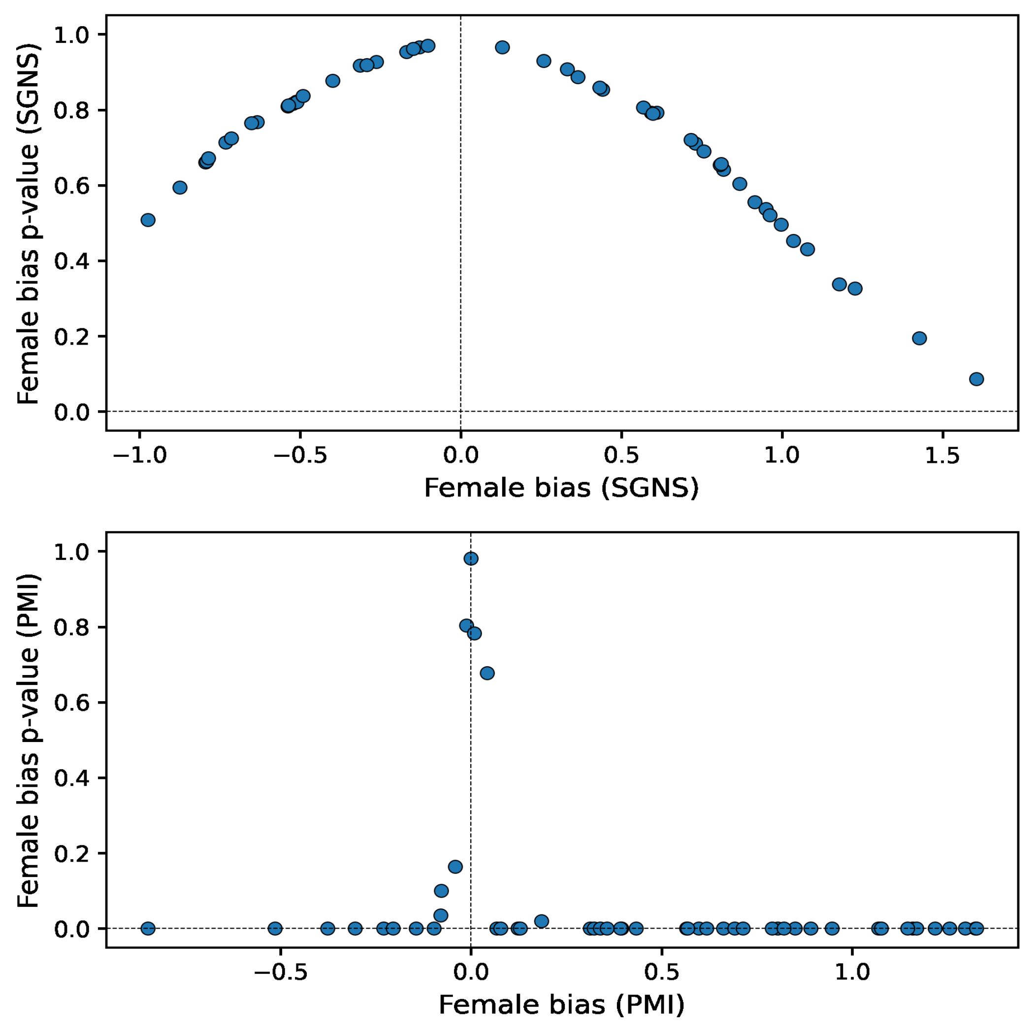
Figure 1: permutation p-values of $\text{Bias}_{\text{WE}}$ with SGNS vs. the value of $\text{Bias}_{\text{WE}}$ with SGNS (top panel), and $\log\text{OR}$ test p-values of $\text{Bias}_{\operatorname{PMI}}$ vs. the value of $\text{Bias}_{\operatorname{PMI}}$ (bottom panel) of androgynous names in Wikipedia.

In Figure 1 we compare the p-values of the permutation test of $\text{Bias}_{\text{WE}}$ with SGNS, with the p-values of the log odds ratio test of $\text{Bias}_{\operatorname{PMI}}$ for the Names-gender test conducted in Wikipedia. A Benjamini-Hochberg correction was applied to the p-values obtained by both methods to account for multiple comparisons (Benjamini and Hochberg, 1995). Appendix F.2 shows this example is consistent with the rest of the experiments.

In this example, only the word with the highest $\text{Bias}_{\text{WE}}$ is significantly different from zero at a 0.10 significance level. In contrast, most words have a $\text{Bias}_{\operatorname{PMI}}$ significantly different from zero, with the exception of some points with bias values close to zero. This is because the procedures that compute p-values for each type of metric capture essentially different types of variability (see section 6.2).

6 Discussion

6.1 Interpretability

Although there are studies on how word vector spaces are formed (Levy and Goldberg, 2014; Levy et al., 2015; Ethayarajh et al., 2019) and on the biases they encode (Bolukbasi et al., 2016; Zhao et al., 2017; Gonen and Goldberg, 2019), there is no transparent interpretation of the embedding-based bias metrics in terms of co-occurrences of words in the texts.

In contrast, $\text{Bias}_{\operatorname{PMI}}$ can be expressed intrinsically in terms of conditional probabilities (equation 5). The bias is interpreted as the logarithm of how much more likely it is to find words in $C$ in the context of words in $A$ than in the context of words in $B$. For example, in the Wikipedia corpus the female $\text{Bias}_{\operatorname{PMI}}$ of word nurse is 1.3172, thus,

$$\frac{P(nurse|A)}{P(nurse|B)}=\exp\,1.3172=3.7330.$$

This means that it is 273.30% more likely to find the word nurse in the context of female words ($A$) than in the context of male words ($B$).

To the lack of interpretability of $\text{Bias}_{\text{WE}}$ contributes the fact that SGNS and GloVe can capture word associations of second order or higher (Altszyler et al., 2018; Schlechtweg et al., 2019), whereas $\operatorname{PMI}$ is strictly a first-order association metric. When embeddings are used to measure biases, it is not possible to tell whether the results are due to widespread first-order co-occurrences or are derived from obscure higher-order co-occurrences (Brunet et al., 2019; Rekabsaz et al., 2021).

For instance, in OpenSubtitles, the $\text{Bias}_{\text{PMI}}$ of the word evil equals $-0.25$, indicating a higher likelihood of appearing in the context of male context words ($B$) compared to female ones ($A$). Conversely, $\text{Bias}_{\text{SGNS}}=0.23$. Even if this stands for female bias, it is difficult to understand the exact source of this result since it is influenced by second and higher-order co-occurrences. Moreover, in recent research we demonstrated that $\text{Bias}_{\text{WE}}$ can also yield misleading results by inadvertently capturing disparities in the frequencies of context words (Valentini et al., 2022).

Nevertheless, bias metrics that capture second-order associations have the advantage of managing data sparsity. Since word embeddings can capture synonymy, when data is sparse it might not be necessary to include all related words to the concepts of interest in order to measure meaningful biases. In the case of our first-order metric, this problem must be addressed by increasing word lists with synonyms and forms of the words of interest.

To illustrate this, let’s consider the case of the words nourish and nurture, which have different frequencies in the Wikipedia corpus ($700$ and $3,000$, respectively). With $\text{Bias}_{\text{PMI}}$, we obtain a bias of $0.33$ for nurture (p-value $<10^{-4}$). However, if we had used its less frequent synonym nourish instead, the $\text{Bias}_{\text{PMI}}$ would have been $-0.10$ and not statistically significant (p-value $\approx 0.66$). Here we would not have been able to determine whether there is actually no bias or if there is insufficient data. This shows that it is generally advisable to include all pertinent synonyms and variations of the term whose bias we are trying to measure.

6.2 Statistical inference

The p-values, standard errors and confidence intervals of the $\log\text{OR}$ approximation are fundamentally different from the ones estimated for $\text{Bias}_{\text{WE}}$ through permutations and bootstrap. The uncertainty quantified for $\text{Bias}_{\operatorname{PMI}}$ captures the variability of the underlying data generating process i.e. the one induced by the randomness of co-occurrence counts as random quantities. In contrast, the estimates for $\text{Bias}_{\operatorname{WE}}$ only consider the variability across the sets of context words. This means that multiple words must be chosen so that inference can be conducted. In fact, whenever $A$ and $B$ are single-word lists, there is no way of estimating uncertainty for $\text{Bias}_{\operatorname{WE}}$ with these methods, whereas it is perfectly feasible for $\text{Bias}_{\operatorname{PMI}}$.

As far as we know, we are the first to provide a simple and efficient way of evaluating the statistical significance of bias. This is especially important in Computational Social Science, for which it is useful to have not only a reliable metric to quantify stereotypes but also a reliable tool to measure uncertainty i.e. to know up to what degree the measured values might have been due to statistical fluctuation. Meaningful statistical tests and confidence intervals that capture the variability that really matters are therefore essential.

7 Conclusion

We presented a PMI-based metric to quantify biases in texts, which (a) allows for simple and computationally inexpensive statistical inference, (b) has a simple interpretation in terms of word co-occurrences, and (c) is explicit and transparent in the associations that it is quantifying, since it captures exclusively first-order co-occurrences. Our method produces similar results to the GloVe-based and SGNS-based metrics in experiments which compare gender biases measured in large corpora to the gender gaps of independent empirical data.

Limitations

We replicate three well-known experiments in the gender bias literature, where bias is measured according to a binary female vs. male view. This choice ignores other views of gender but eases the presentation of the frameworks.

We only use two corpora and three datasets which by no means capture the biases of all the people speaking or writing in the English language. Moreover, we don’t experiment with different corpus sizes, a more diversified set of corpora or more bias types. We hope to explore this in future work.

The hyperparameters of the models have not been varied, using their default values. This replicates the standard experimental setting used in the literature. Since there are no ground truths when measuring biases (that is, there are no annotations with the amount of bias of words in large corpora), hyperparameters are usually set to their default values.

Appendix A Contingency table of co-occurrences

$\text{Bias}_{\operatorname{PMI}}$ is computed with the co-occurrences between the groups of words $A$, $B$ and $C$. These can be represented with the following contingency table:

	$C$	$not\;C$	Total
$A$	$f_{A,C}$	$f_{A,nC}$	$f_{A,C}$+$f_{A,nC}$
$B$	$f_{B,C}$	$f_{B,nC}$	$f_{B,C}$+$f_{B,nC}$

Table 2: Contingency table of words co-occurrences

This contains, for example, how many times words in $A$ appear in the context of words in $C$ ($f_{A,C}$) and how many times they do not ($f_{A,nC}$).

Appendix B Statistical inference for $\text{Bias}_{\operatorname{PMI}}$

The distribution of the log odds ratio (equation 7) converges to normality (Agresti, 2003). Its 95% confidence interval is given by

$$CI_{95\%}\big{(}\text{Bias}_{\operatorname{PMI}}\big{)}=\text{Bias}_{\operatorname{PMI}}\pm 1.96\,SE$$

with

$$SE = \sqrt{\frac{1}{f_{A,C}}+\frac{1}{f_{B,C}}+\frac{1}{f_{A,nC}}+\frac{1}{f_{B,nC}}}$$

$$\approx \sqrt{\frac{1}{f_{A,C}}+\frac{1}{f_{B,C}}}$$

This last approximation considers condition 6.

We can test the null hypothesis that the log odds ratio is 0 (absence of bias) with a standard Z-test, whereby the two-sided p-value is computed with $2P(\text{Z}<-|\text{Bias}_{\operatorname{PMI}}|/SE)$, where Z is a standard normal random variable.

Appendix C Datasets

For the occupations-gender and names-gender experiments, the female proportions for names and occupations in the U.S. were extracted from the datasets provided by Will Lowe’s cbn R library , which contains tools for replicating Caliskan et al. (2017). We used the 50 names and 44 occupations available in this source.

The original Glasgow Norms comprise 5,553 English words. Individuals from the University of Glasgow were asked to measure the degree to which each word is associated with male or female behavior on a scale from 1 (very feminine) to 7 (very masculine). Following Lewis and Lupyan (2020), we average the norms of homonyms and compute $8-rating$ to flip the scale so that it represents femaleness according to human judgement. 4,668 words from the original list overlapped with OpenSubtitle’s vocabulary, and 4,642 words overlapped with the Wikipedia vocabulary.

Appendix D Corpora

The Wikipedia corpus was built from the August 2014 dump, licensed under CC BY-SA 3.0. We removed articles with less than 50 tokens.

The OpenSubtitles corpus (Lison and Tiedemann, 2016) includes English subtitles from movies and TV shows and was built with the aid of the subs2vec Python package with MIT License (van Paridon and Thompson, 2021).

Appendix E Model training

We ignore words with less than 100 occurrences, resulting in a vocabulary of 172,748 words for Wikipedia and 128,974 words for OpenSubtitles.

We use a window size of 10 in all models and apply "dirty" subsampling i.e. out-of-vocabulary tokens are removed before the corpus is processed into word-context pairs (Levy et al., 2015).

Word embeddings with 300 dimensions are trained with SGNS and GloVe. For SGNS we use the word2vec implementation of Gensim 4.1.2 licensed under GNU LGPLv2.1 (Řehůřek and Sojka, 2010) with default hyperparameters. GloVe is trained with the original implementation (Pennington et al., 2014) with version 1.2 (Apache License, Version 2.0) with 100 iterations. This version uses by default additive word representations, in which each word embedding is the sum of its corresponding context and word vectors.

For PMI, we count co-occurrences with the GloVe module (Pennington et al., 2014) with version 1.2 and set the smoothing parameter $\epsilon$ to 0.5.

We ran all experiments on a desktop machine with 4 cores Intel Core i5-4460 CPU and 32 GB RAM. Training times were around 1 hour per epoch with SGNS and 5 minutes per iteration with GloVe. Co-occurrence counts used for PMI were obtained in around 20 minutes with GloVe.

Appendix F Results

F.1 Experiments

In Figures 2, 3 and 4 we display the scatter plots of the three experiments described in section 4 for the Wikipedia corpus. The findings for OpenSubtitles are qualitatively the same and we exclude the plots for simplicity.

The vertical axes represent the female vs. masculine bias measures based on PMI (left panels), GloVe (middle panels), and SGNS (right panels). Dashed lines represent linear regressions. In the second row, the bias standard error was taken into account as weights in the regression, and error bars are confidence intervals.

All unweighted and weighted correlation coefficients in Table 1 are significantly different from zero at the 0.0001 level.

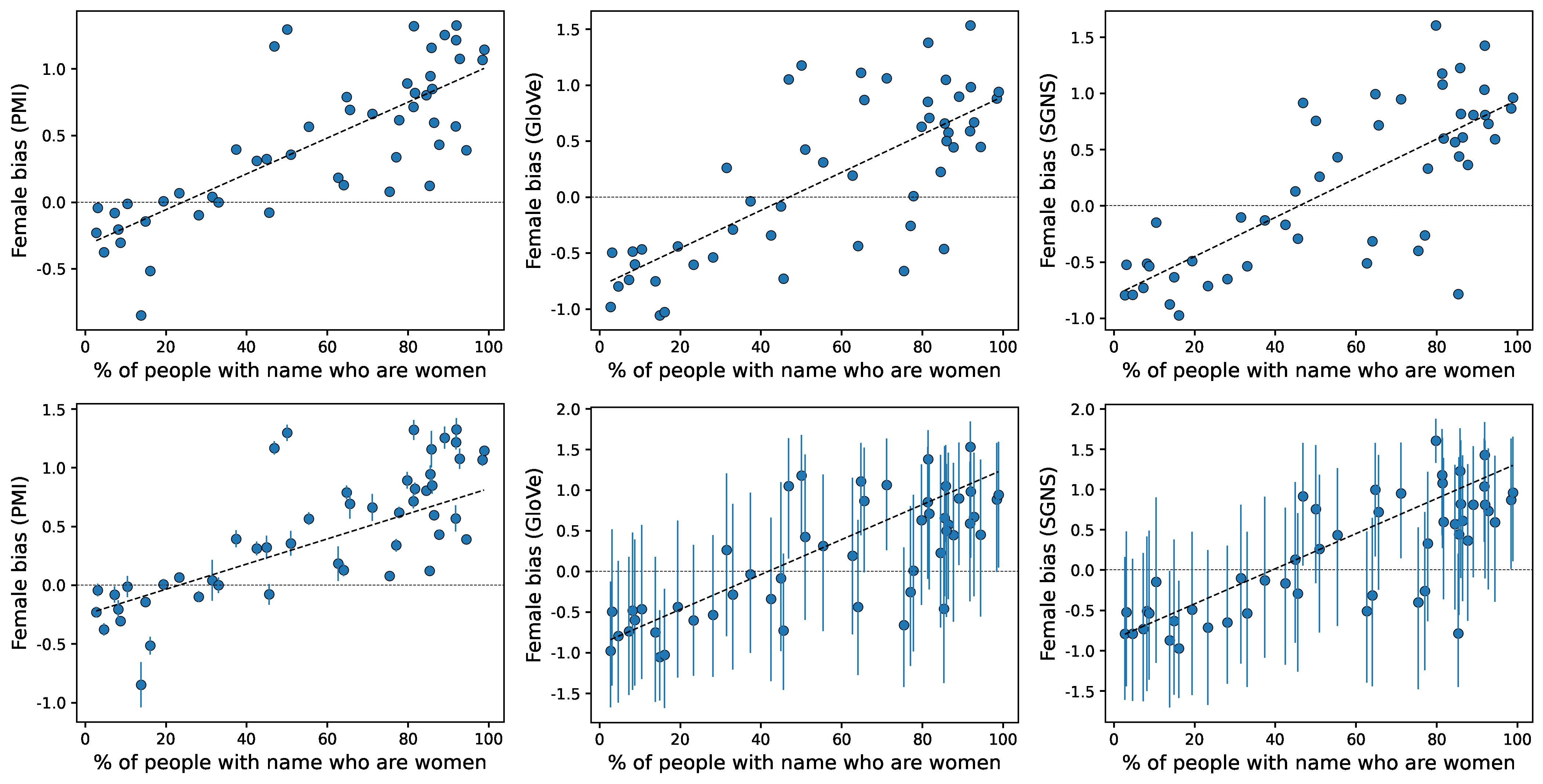
Figure 2: Names-gender experiments in Wikipedia. Horizontal axes represent the percentage of people with each name who are women as measured in the 1990 U.S. census.

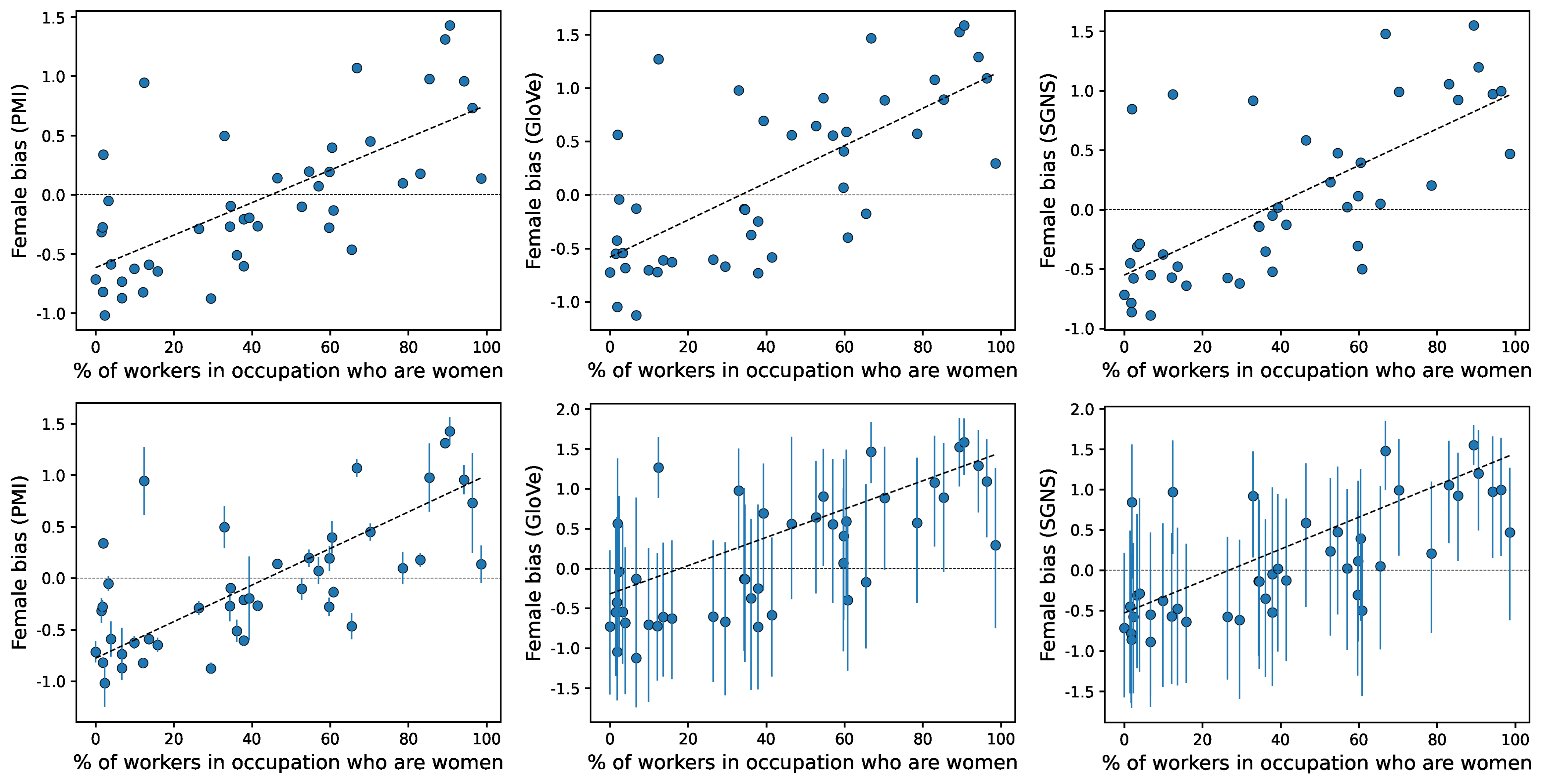
Figure 3: Occupations-gender experiments in Wikipedia. Horizontal axes represent the percentage of women employed in each occupation in 2015 according to the U.S. Bureau of Labor Statistics.

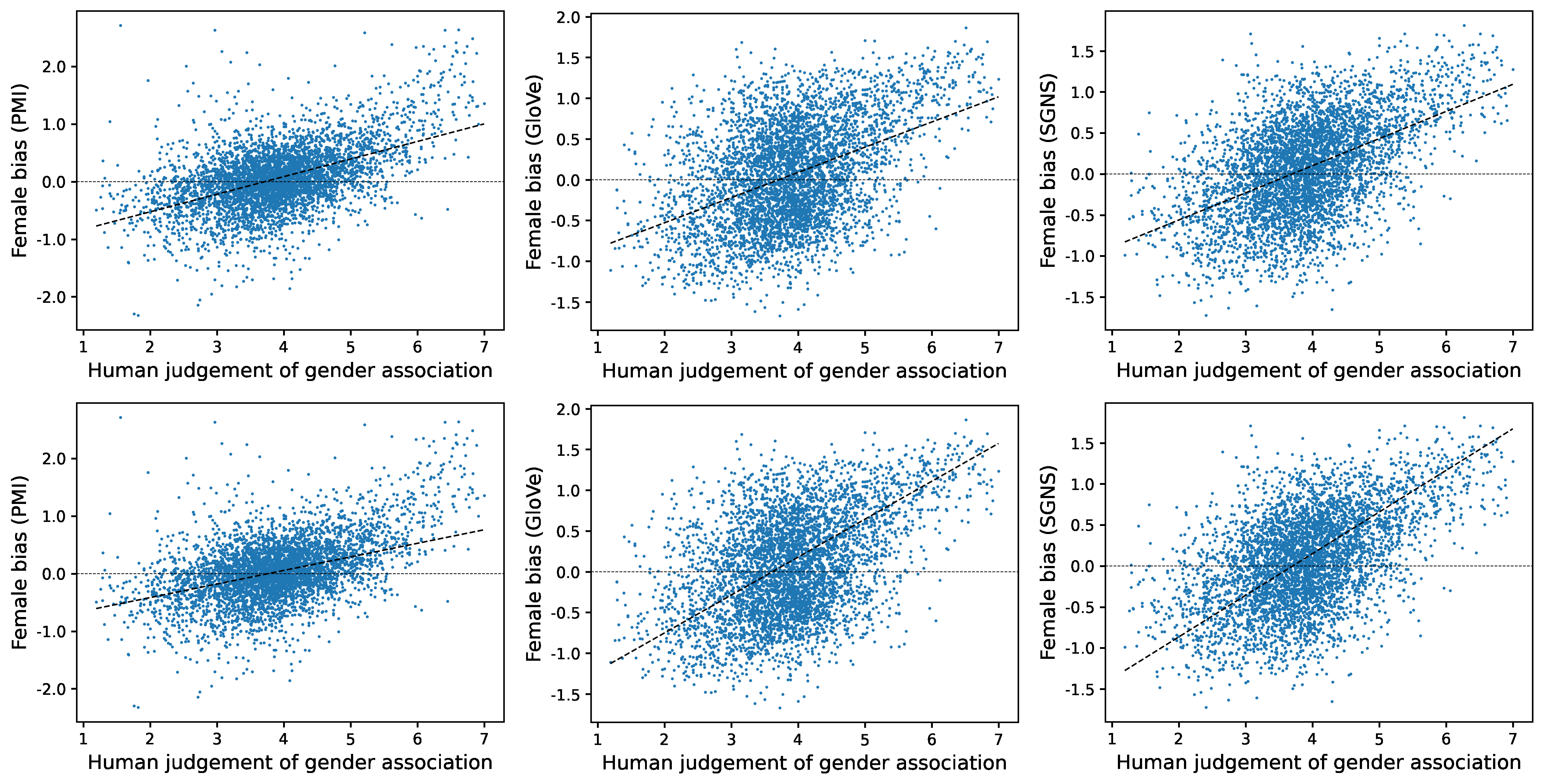
Figure 4: Norms-gender experiments in Wikipedia. Horizontal axes represent the Glasgow Norm of each word. Confidence intervals are not displayed in the second row to avoid overplotting.

F.2 p-values

Figure 5 shows the corrected p-values for the gender bias of each word in the vertical axes vs. the value of the bias in the horizontal axes. p-values for SGNS and GloVe result from permutations tests whereas PMI uses the log odds ratio test. All p-values have been corrected with Benjamini-Hochberg separately for each setting. The plots for OpenSubtitles are very similar and are excluded for simplicity.

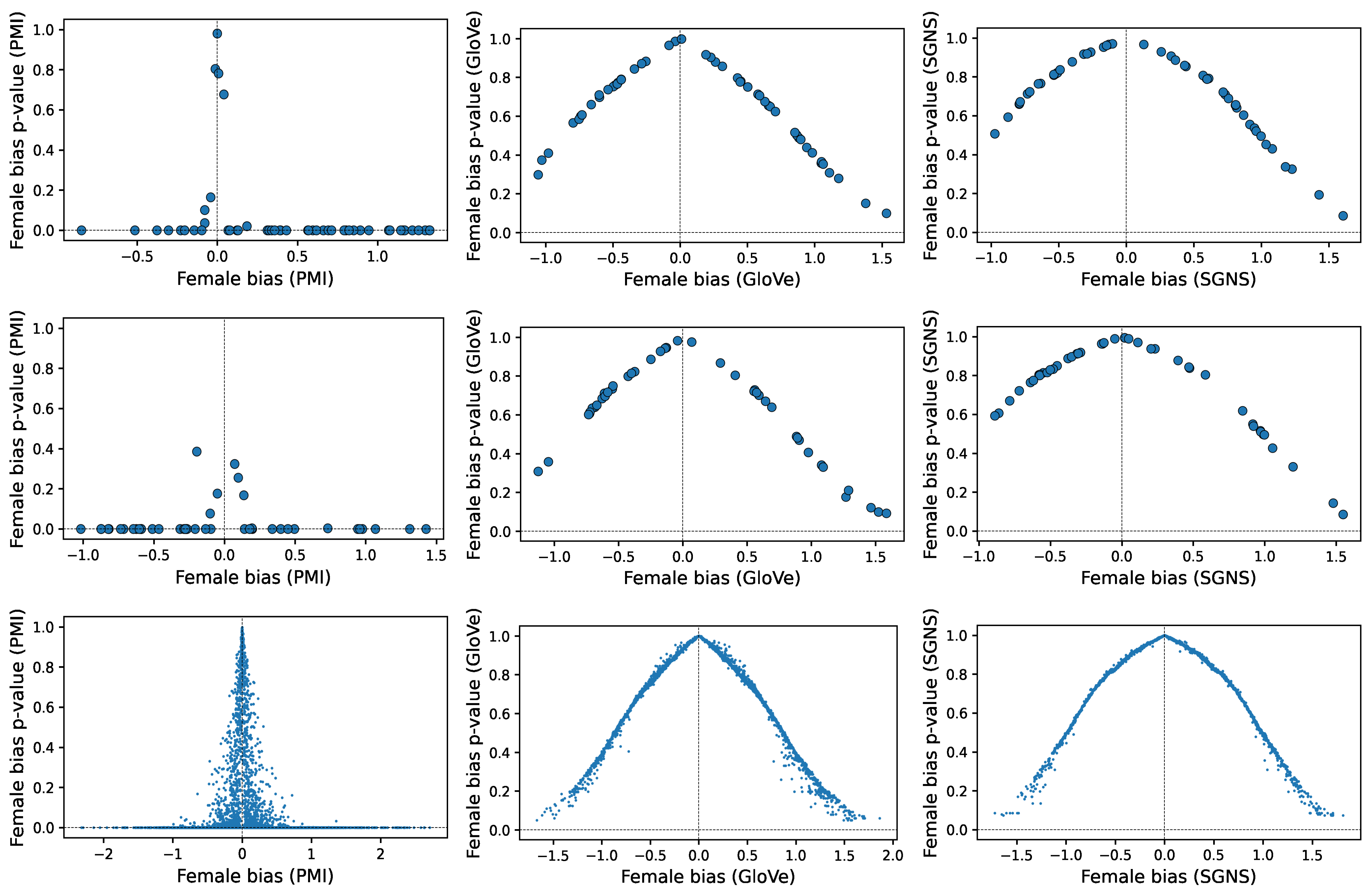
Figure 5: Female vs. male bias p-values of the names-gender (row 1), occupations-gender (row 2) and norms-gender (row 3) experiments in Wikipedia.

References

- Agresti (2003) Alan Agresti. 2003. Categorical data analysis, volume 482. John Wiley & Sons.
- Aka et al. (2021) Osman Aka, Ken Burke, Alex Bauerle, Christina Greer, and Margaret Mitchell. 2021. Measuring model biases in the absence of ground truth. In Proceedings of the 2021 AAAI/ACM Conference on AI, Ethics, and Society. ACM.
- Altszyler et al. (2018) Edgar Altszyler, Mariano Sigman, and Diego Fernández Slezak. 2018. Corpus specificity in LSA and word2vec: The role of out-of-domain documents. In Proceedings of The Third Workshop on Representation Learning for NLP, pages 1–10, Melbourne, Australia. Association for Computational Linguistics.
- Benjamini and Hochberg (1995) Yoav Benjamini and Yosef Hochberg. 1995. Controlling the false discovery rate: A practical and powerful approach to multiple testing. Journal of the Royal Statistical Society Series B (Methodological), 57(1):289–300.
- Bolukbasi et al. (2016) Tolga Bolukbasi, Kai-Wei Chang, James Y Zou, Venkatesh Saligrama, and Adam T Kalai. 2016. Man is to computer programmer as woman is to homemaker? debiasing word embeddings. In Advances in Neural Information Processing Systems, volume 29. Curran Associates, Inc.
- Bordia and Bowman (2019) Shikha Bordia and Samuel R. Bowman. 2019. Identifying and reducing gender bias in word-level language models. In Proceedings of the 2019 Conference of the North American Chapter of the Association for Computational Linguistics: Student Research Workshop, pages 7–15, Minneapolis, Minnesota. Association for Computational Linguistics.
- Brunet et al. (2019) Marc-Etienne Brunet, Colleen Alkalay-Houlihan, Ashton Anderson, and Richard Zemel. 2019. Understanding the origins of bias in word embeddings. In Proceedings of the 36th International Conference on Machine Learning, volume 97 of Proceedings of Machine Learning Research, pages 803–811. PMLR.
- Caliskan et al. (2017) Aylin Caliskan, Joanna J. Bryson, and Arvind Narayanan. 2017. Semantics derived automatically from language corpora contain human-like biases. Science, 356(6334):183–186.
- Charlesworth et al. (2021) Tessa ES Charlesworth, Victor Yang, Thomas C Mann, Benedek Kurdi, and Mahzarin R Banaji. 2021. Gender stereotypes in natural language: Word embeddings show robust consistency across child and adult language corpora of more than 65 million words. Psychological Science, 32(2):218–240.
- Church and Hanks (1990) Kenneth Ward Church and Patrick Hanks. 1990. Word association norms, mutual information, and lexicography. Computational Linguistics, 16(1):22–29.
- Davison and Hinkley (1997) A. C. Davison and D. V. Hinkley. 1997. Bootstrap Methods and their Application. Cambridge Series in Statistical and Probabilistic Mathematics. Cambridge University Press.
- DeFranza et al. (2020) David DeFranza, Himanshu Mishra, and Arul Mishra. 2020. How language shapes prejudice against women: An examination across 45 world languages. Journal of Personality and Social Psychology, 119(1):7–22.
- Ethayarajh et al. (2019) Kawin Ethayarajh, David Duvenaud, and Graeme Hirst. 2019. Understanding undesirable word embedding associations. In Proceedings of the 57th Annual Meeting of the Association for Computational Linguistics, pages 1696–1705, Florence, Italy. Association for Computational Linguistics.
- Gálvez et al. (2019) Ramiro H. Gálvez, Valeria Tiffenberg, and Edgar Altszyler. 2019. Half a century of stereotyping associations between gender and intellectual ability in films. Sex Roles, 81(9):643–654.
- Garg et al. (2018) Nikhil Garg, Londa Schiebinger, Dan Jurafsky, and James Zou. 2018. Word embeddings quantify 100 years of gender and ethnic stereotypes. Proceedings of the National Academy of Sciences, 115(16):E3635–E3644.
- Gonen and Goldberg (2019) Hila Gonen and Yoav Goldberg. 2019. Lipstick on a pig: Debiasing methods cover up systematic gender biases in word embeddings but do not remove them. In Proceedings of the 2019 Conference of the North American Chapter of the Association for Computational Linguistics: Human Language Technologies, Volume 1 (Long and Short Papers), pages 609–614, Minneapolis, Minnesota. Association for Computational Linguistics.
- Jones et al. (2020) Jason J. Jones, Mohammad Ruhul Amin, Jessica Kim, and Steven Skiena. 2020. Stereotypical gender associations in language have decreased over time. Sociological Science, 7(1):1–35.
- Jurafsky and Martin (2009) Daniel Jurafsky and James H. Martin. 2009. Speech and Language Processing (2nd Edition). Prentice-Hall, Inc., USA.
- Kozlowski et al. (2019) Austin C. Kozlowski, Matt Taddy, and James A. Evans. 2019. The geometry of culture: Analyzing the meanings of class through word embeddings. American Sociological Review, 84(5):905–949.
- Levy and Goldberg (2014) Omer Levy and Yoav Goldberg. 2014. Neural word embedding as implicit matrix factorization. In Advances in Neural Information Processing Systems, volume 27. Curran Associates, Inc.
- Levy et al. (2015) Omer Levy, Yoav Goldberg, and Ido Dagan. 2015. Improving distributional similarity with lessons learned from word embeddings. Transactions of the Association for Computational Linguistics, 3:211–225.
- Lewis and Lupyan (2020) Molly Lewis and Gary Lupyan. 2020. Gender stereotypes are reflected in the distributional structure of 25 languages. Nature Human Behaviour, 4(10):1021–1028.
- Lison and Tiedemann (2016) Pierre Lison and Jörg Tiedemann. 2016. OpenSubtitles2016: Extracting large parallel corpora from movie and TV subtitles. In Proceedings of the Tenth International Conference on Language Resources and Evaluation (LREC’16), pages 923–929, Portorož, Slovenia. European Language Resources Association (ELRA).
- North et al. (2002) B. V. North, D. Curtis, and P. C. Sham. 2002. A note on the calculation of empirical p values from monte carlo procedures. The American Journal of Human Genetics, 71(2):439–441.
- Pennington et al. (2014) Jeffrey Pennington, Richard Socher, and Christopher D. Manning. 2014. Glove: Global vectors for word representation. In Empirical Methods in Natural Language Processing (EMNLP), pages 1532–1543.
- Řehůřek and Sojka (2010) Radim Řehůřek and Petr Sojka. 2010. Software Framework for Topic Modelling with Large Corpora. In Proceedings of the LREC 2010 Workshop on New Challenges for NLP Frameworks, pages 45–50, Valletta, Malta. ELRA. http://is.muni.cz/publication/884893/en.
- Rekabsaz et al. (2021) Navid Rekabsaz, Robert West, James Henderson, and Allan Hanbury. 2021. Measuring societal biases from text corpora with smoothed first-order co-occurrence. Computing Research Repository, arXiv:1812.10424.
- Schlechtweg et al. (2019) Dominik Schlechtweg, Cennet Oguz, and Sabine Schulte im Walde. 2019. Second-order co-occurrence sensitivity of skip-gram with negative sampling. In Proceedings of the 2019 ACL Workshop BlackboxNLP: Analyzing and Interpreting Neural Networks for NLP, pages 24–30, Florence, Italy. Association for Computational Linguistics.
- Scott et al. (2019) Graham G Scott, Anne Keitel, Marc Becirspahic, Bo Yao, and Sara C Sereno. 2019. The Glasgow Norms: Ratings of 5,500 words on nine scales. Behavior Research Methods, 51:1258–1270.
- Valentini et al. (2022) Francisco Valentini, Germán Rosati, Diego Fernandez Slezak, and Edgar Altszyler. 2022. The undesirable dependence on frequency of gender bias metrics based on word embeddings. In Findings of the Association for Computational Linguistics: EMNLP 2022. Association for Computational Linguistics.
- van Paridon and Thompson (2021) Jeroen van Paridon and Bill Thompson. 2021. subs2vec: Word embeddings from subtitles in 55 languages. Behavior Research Methods, 53(2):629–655.
- Zhao et al. (2017) Jieyu Zhao, Tianlu Wang, Mark Yatskar, Vicente Ordonez, and Kai-Wei Chang. 2017. Men also like shopping: Reducing gender bias amplification using corpus-level constraints. In Proceedings of the 2017 Conference on Empirical Methods in Natural Language Processing, pages 2979–2989, Copenhagen, Denmark. Association for Computational Linguistics.