Mitigating Hand Blockage with Non-Directional Beamforming Codebooks

Abstract

Hand blockage leads to significant performance impairments at millimeter wave carrier frequencies. A number of prior works have characterized the loss in signal strength with the hand using studies with horn antennas and form-factor user equipments (UEs). However, the impact of the hand on the effective phase response seen by the antenna elements has not been studied so far. Towards this goal, we consider a measurement framework that uses a hand phantom holding the UE in relaxed positions reflective of talk mode, watching videos, and playing games. We first study the impact of blockage on a directional beam steering codebook. The tight phase relationship across antenna elements needed to steer beams leads to a significant performance degradation as the hand surface can distort the observed amplitudes and phases across the antenna elements, which cannot be matched by this codebook. To overcome this loss, we propose a non-directional beamforming codebook made of amplitudes and/or quantized phases with both these quantities estimated as necessary. Theoretical as well as numerical studies show that the proposed codebook can de-randomize the phase distortions induced by the hand and coherently combine the energy across antenna elements and thus help in mitigating hand blockage losses.

I Introduction

Millimeter wave systems have significantly matured over the last five years with advances in technological aspects, low-complexity and low-cost manufacturing as well as in standard specifications and regulatory support. Enabled by these advances, the first wave of commercial deployments in the $28$ and $39$ GHz regimes are now currently available in the market across multiple geographies. Yet, a number of basic issues in terms of practical viability of systems operating at millimeter wave frequencies are still not very well understood. One such issue is the question of hand blockage that can significantly impair link margins at millimeter wave frequencies.

Modeling of blockage has received significant attention over the last few years. For example, ray-tracing based blockage models have been proposed for 802.11(ad) [2] as well as for the Third Generation Partnership Project (3GPP) Fifth Generation-New Radio (5G-NR) systems [3]. In particular, the 3GPP 5G-NR model captures the spatial region of blockage in a local coordinate system around the user equipment (UE) in the Portrait and Landscape modes with a $30$ dB flat loss assumed over this region. It is now understood that the $30$ dB loss is pessimistic and is mostly a reflection of horn antenna studies such as [4, 5] that were used to initiate discussions on the blockage model at 3GPP. More recent studies that use phased array systems show a considerably smaller blockage loss than $30$ dB.

For example, blockage studies at $15$ GHz with subarray/antenna module diversity that allows module switching across different paths/clusters in the channel is shown to result in reduced blockage losses [6, 7]. A similar study with ray tracing is performed in [8] for $15$ and $28$ GHz systems. Creeping waves and diffraction of signals are attributed as reasons for reduced blockage losses at $28$ GHz in [9]. Simulated studies of hand blockage losses with an $8\times 1$ linear antenna array and a $10\times 1$ irregular antenna array in a $28$ GHz form-factor phone design are presented in [10] and [11], respectively. In both works, reduced blockage losses relative to the 3GPP model are reported. Simulation studies of the finger at $60$ GHz are reported in [12, 13] and a large loss variation is reported depending on the finger placement on/near the antenna module. User effects on the power variation are reported for $21.5$ GHz systems in [14] with many scenarios of loss and some scenarios of gain observed. Phased array vs. switched diversity array tradeoffs with hand and body blockage are studied in [15] and the regime where each approach is better is quantified.

In some of our prior works [16, 17], a $28$ GHz form-factor prototype with 3GPP-type beam management solution was used to study the impact of blockage losses. A median blockage loss of no more than $\approx 15$ dB was reported even with the hardest hand grip and this reduced loss was attributed to the increased beamwidth of the beam ($\approx 25^{\sf o}$ for a $4\times 1$ array) relative to a horn antenna setup ($\approx 8^{\sf o}$ to $10^{\sf o}$). The increased beamwidth allows more energy to be collected by the phased array even with the presence of a hand thereby reducing the effective blockage losses. An important caveat common to these studies is that they are either based on ray-tracing or electromagnetic simulation studies, or with experimental prototypes that may/may not be a form-factor implementation.

More recently, measurement based blockage estimates with a commercial grade $28$ GHz UE design are reported in [18]. Here, loss of less than $10$ dB and $20$ dB are estimated for loose and hard hand grips, respectively. Further, it is shown that blockage can lead to reflection-associated gains in certain directions over the sphere and these scenarios are important for loose hand grips. The region of interest (RoI) where blockage loss/gain is relevant is identified and spherical coverage improvement with blockage in loose hand grip mode is formally characterized.

In general, if a blockage-driven link deterioration is seen, the UE can mitigate these losses by either [17]:

• Switching to a better path/cluster in the channel, which implicitly assumes multiple capabilities at the UE side, or

• Living with the deteriorated path and the concomitant link degradation.

For the first approach (beam switching) to work, we implicitly rely on a potentially densified network with viable paths/clusters from multiple transmit nodes, a rich multipath channel with the connected (or potentially switching) transmit node, multiple antenna modules and associated radio frequency integrated circuits (RFICs) to allow the UE to switch to a different path/cluster, beam switching latencies that are not disruptive to communications, and coordination with the transmit node to allow beam switching [17]. In this work, we propose an additional and entirely different mitigation strategy to add to this arsenal.

Towards this goal, we first report controlled blockage measurements with a commercial grade $28$ GHz system using a $4\times 1$ dual-polarized patch array with a commercial grade hand phantom in an anechoic chamber. In contrast to all the prior works that focus only on the amplitude response with blockage, we record the complete electric field (or array response) measurements that includes both amplitudes and phases in Freespace over the sphere. This set of benchmark measurements are then compared with the complete hand blockage measurements using an anthropomorphic hand phantom in four scenarios where the hand phantom is placed on top of the antenna module with one or two fingers blocking/obstructing the antenna elements, and where the hand phantom is placed $1$ mm away from the antenna array with signals blocked using one or two fingers. These scenarios capture practical hand holdings such as those used in talk mode, watching videos, playing video games, etc.

We first consider an ideal/optimal maximum ratio combining (MRC) scheme that can tune the amplitudes and phases across all the angles in the RoI with infinite precision. With this approach, we show that median blockage losses in the range of $2.7$ to $4.5$ dB (larger losses corresponding to the two fingers of the phantom hand on top of the antenna module) are seen with the $90$-th percentile losses being in the range of $7.1$ to $11.6$ dB. Since infinite-precision codebooks are not practically viable, we then consider a static beam steering codebook of size-$4$ (commensurate with the size of the antenna array). We show that this approach incurs a median and $90$-th percentile losses in the range of $2.0$ to $2.3$ dB and $3.7$ to $3.9$ dB, respectively. Bridging this gap in performance with any other approach is important for the evolution of millimeter wave technology.

In this direction, we carefully study the amplitude and phase response with the hand phantom and illustrate that multiple reflections from the different parts of the hand lead to a randomization of the phase response as seen in the Freespace mode. As a result, a static codebook with a phase response tailored to steer beams in specific directions may not lead to a constructive addition of signals seen by the different antenna elements. This observation motivates a codebook enhancement strategy that searches over different amplitude and phase shifter combinations so that a good choice of beam weights can be arrived at. This good choice leads to an appropriate weighting of the antenna elements to de-randomize the phases. Such an approach is shown to theoretically improve the beamforming performance significantly. This result is also verified via measurements and median and $90$-th percentile losses (relative to MRC) on the order of $\approx 0.35$ and $\approx 0.85$ dB, respectively, are reported. Note that these loss ranges are far smaller than those seen with a static codebook strategy.

This paper is organized as follows. Section II describes the measurement setup including the experiments performed in this paper. Sections III and IV study the impact of blockage at a single antenna level and with beamforming, respectively. Section V proposes a mitigation strategy to handle blockage and the intuitive motivation behind this specific choice. Theoretical and numerical studies of the proposed approach are also considered with concluding remarks in Section VI.

II Measurement Setup

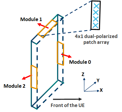
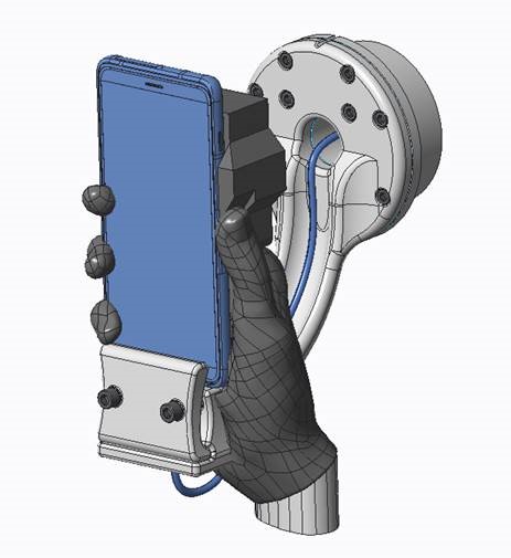
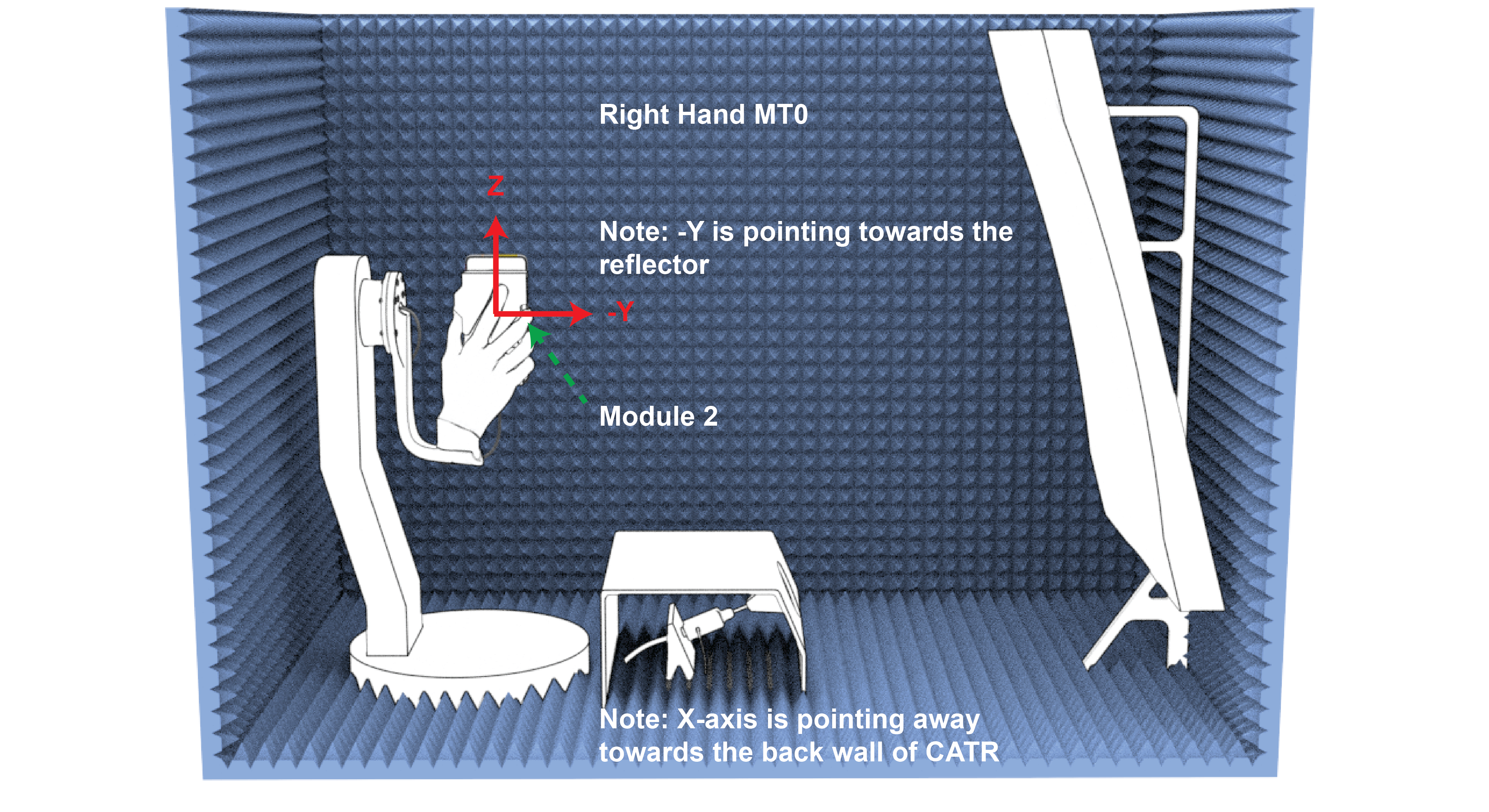
(a)	(b)	(c)

Figure 1: (a) Illustration of UE with antenna module structure. (b) Illustration of the hand phantom holding the UE in (b) a stand-alone setup and (c) with the measurement setup in the chamber.

The UE considered in this study is equipped with a commercial grade millimeter wave modem operating at $28$ GHz and using a 3GPP Rel. $15$ and $16$ standard specifications-compliant software stack that performs intelligent beamforming and beam tracking. From an antenna module perspective, as illustrated in Fig. 1(a), the UE consists of three modules, denoted as Modules $0$ to $2$, which are placed on the right long edge, top short edge and left long edge, respectively, as seen from the front of the UE. From a beamforming perspective, each antenna module has a $4\times 1$ dual-polarized patch array that allows dual-polarized transmissions via two radio frequency (RF) chains at $28$ GHz.

For the studies in this paper, we use a commercial grade anthropomorphic hand phantom [19] which is specifically designed for evaluating and optimizing over-the-air (OTA) performance of ultra-wide mobile phone devices (defined as having a width between $72$ and $92$ mm) such as the one considered in this paper. The hand phantom is manufactured using a silicone-carbon-based mixture with material properties conforming to the Cellular Telecommunications Industry Association (CTIA) definitions and standards for hand phantoms. The use of a special low-loss silicone coating extends its useable frequency range from $3$ GHz to $110$ GHz. For the accuracy and reliability of the evaluation results, as illustrated in Fig. 1(b), the UE is placed on a specially designed holding fixture that does not block the antenna modules. This fixture is made of a low-loss production grade thermoplastic material and is 3D-printed using fused deposition modeling technology [20].

While hand blockage studies are best performed with a true human holding the UE [18], avoiding the conflation of hand blockage effects with that of body blockage effects as well as exposure considerations suggest that studies with a hand phantom are a good proxy to capturing the true hand blockage effects. Therefore, to study the impact of hand blockage, four controlled studies corresponding to specific hand phantom positions are considered in this paper. These four positions include:

• Hand phantom on top of the antenna elements (that is, a $0$ mm air gap between the antenna module and the phantom) with either $1$ or $2$ fingers blocking/obstructing the antenna elements of the antenna module as illustrated in Fig. 1, and

• Hand phantom with a $1$ mm air gap from the antenna module with either $1$ or $2$ fingers obstructing the radiation of the antenna module.

The $1$ mm air gap is introduced (and enforced) by placing a small rectangular low-loss foam material between the tip of the finger(s) and the antenna module. The $0$ mm air gap scenario is expected to capture a hand holding in talk mode as some of the fingers are expected to be touching the antenna module when a user talks on the phone. The $1$ mm air gap scenario is expected to capture a user playing a game with a small air gap between the fingers and the UE. These illustrative (but non-limiting) examples are thus expected to cover an interesting gamut of practical applications. In the studies considered in this paper, the hand phantom is placed over Module 2 (antenna module of interest) with a boresight direction of -Y axis (left long edge), as illustrated in Fig. 1(c).

For 3GPP-compliant OTA tests, the anechoic chamber uses a Compact Antenna Test Range (CATR) method for far-field electromagnetic wave characterization. In this setup, a parabolic reflector is used to collimate radiation at a test probe (as illustrated in Fig. 1(c)) [21]. With this setup, automated chamber measurements (without the presence of humans) are conducted to remove the across-human variations and the impact of body blockage in the collected data. Further, a full set of measurements for each antenna element can take a significant amount of time ($18$ to $20$ minutes) and automation of this process allows us to minimize human exposure to electromagnetic wave radiation.

In this process, electric field information (amplitudes and phases) of each of the antenna elements of the $4\times 1$ array are separately collected in different modes of operation (Freespace mode as well as with the hand phantoms correctly installed over the antenna module). Note that the electric field information captures the array response as seen from the UE end including the effects of housing, antenna substrate, metal/plastic, sensors, other electronic components, etc. The performance of different analog beamforming codebook designs are then studied offline (as described in the sequel) with the collected electric field information for all the antenna elements.

III Amplitude Response at Individual Antenna Level

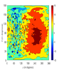
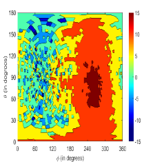
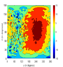
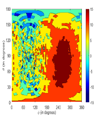
(a)	(b)	(c)	(d)
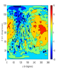
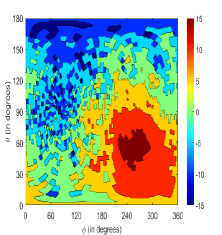
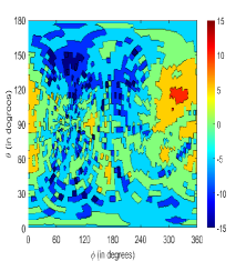
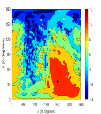
(e)	(f)	(g)	(h)
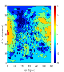
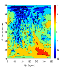
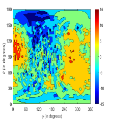
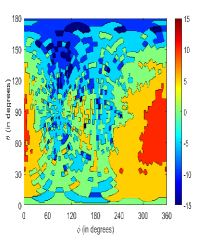
(i)	(j)	(k)	(l)

Figure 2: Contour plots over the sphere of elemental pattern of individual Antennas 0 to 3 (a)-(d) in Freespace, (e)-(h) with $0$ mm air gap and one finger on the module, and (i)-(l) with $0$ mm air gap and two fingers on the module.

Electric field information (amplitudes and phases) that capture the elemental patterns of the four individual antenna elements of the $4\times 1$ array in Freespace are measured in the chamber. These amplitudes and phases are recorded in $5^{\sf o}$ angular steps around the sphere (in azimuth and elevation) in a global coordinate system, which translates to a finite but non-uniform precision in the coordinate system local to the UE. The amplitudes and phases are then extrapolated over a uniform grid of sample points and with this data, the contour plots of the elemental patterns of these four antenna elements in Freespace are plotted in Figs. 2(a)-(d). These plots show that the individual antenna elemental gains peak around $\theta=90^{\sf o}$ and $\phi=270^{\sf o}$ (or -Y axis), as expected from the coordinate system presented in Fig. 1. The elemental patterns have good gains in $\approx 90^{\sf o}\times 120^{\sf o}$ of the sphere, which is also typical of antenna elements at millimeter wave carrier frequencies [22].

For the $0$ mm air gap scenario with one and two fingers on the antenna module, Figs. 2(e)-(h) and Figs. 2(i)-(l) illustrate the elemental patterns, respectively. Clearly, from these figures, we see significant signal strength distortion (re-orientation of the peak direction as well as attenuation across the coverage region) for all the antenna elements with loss in most directions, but occasional gains in some directions. From a visual point-of-view, signal distortions correspond to changes in regions plotted as oceans of red in Figs. 2(a)-(d) in Freespace to regions plotted as orange, green and blue in Figs. 2(e)-(h) and (i)-(l), respectively.

Towards a quantitative study, let $E_{{\sf free},i}(\theta,\phi)$ and $E_{{\sf blockage},i}(\theta,\phi)$ denote the (complete) electric fields of the $i$-th antenna in the $(\theta,\phi)$ direction of the sphere in Freespace and with blockage, respectively. In a more careful comparative analysis of the impact of blockage on the amplitudes seen by the antenna elements, in Figs. 3(a)-(b), we plot $10\cdot\log_{10}\left(\left|\frac{E_{{\sf free},0}(\theta,\phi)}{E_{{\sf blockage},0}(\theta,\phi)}\right|^{2}\right)$ for Antenna 0 over a Region of Interest (RoI) of the sphere in the $0$ mm air gap case with one and two fingers, respectively. The RoI chosen in this study is $[150^{\sf o},\hskip 1.4457pt360^{\sf o})\times[0^{\sf o},\hskip 1.4457pt180^{\sf o})$ in azimuth and elevation, which covers $\approx 58.3\%$ of the sphere. From this plot, we observe that the presence of the hand either leads to significant losses or significant gains, or comparable amplitude responses relative to the Freespace scenario (blue regions in the plots).

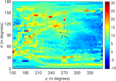
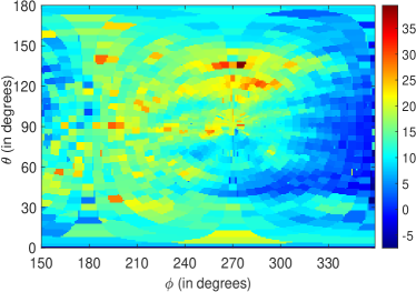
(a)	(b)

Figure 3: Amplitude distortion between the Freespace and blockage scenario with $0$ mm air gap corresponding to (a) one and (b) two fingers.

In the one and two finger cases for the $0$ mm air gap, the finger(s) is/are approximately near Antenna 2 and Antennas 0 and 1, respectively. In the $1$ mm air gap, the finger(s) is/are approximately near Antenna 3 and Antennas 0 and to the left of Antenna 0, respectively. This is captured by the significant distortion in the elemental patterns in these settings. To accurately quantify the blockage losses with different antenna elements in contrast to the naïve RoI as in Fig. 3, we define a RoI over the sphere associated with the $i$-th antenna as follows:

$${\sf RoI}_{i}=\Big{\{}(\theta,\phi)\hskip 1.4457pt:\hskip 1.4457ptG_{{\sf free},i}(\theta,\phi)\geq G_{1}\hskip 3.61371pt{\sf or}\hskip 3.61371ptG_{{\sf blockage},i}(\theta,\phi)\geq G_{2}\Big{\}}$$

where

$$G_{{\sf free},i}(\theta,\phi) = 10\cdot\log_{10}\left(|E_{{\sf free},i}(\theta,\phi)|^{2}\right){\hskip 3.61371pt}{\sf and}$$

$$G_{{\sf blockage},i}(\theta,\phi) = 10\cdot\log_{10}\left(|E_{{\sf blockage},i}(\theta,\phi)|^{2}\right)$$

denote the gains (in dB) of the $i$-th antenna in Freespace and with blockage, respectively. The thresholds $G_{1}$ are $G_{2}$ are defined appropriately (see [18] for a discussion on good choices of thresholds). In general, a small/narrow definition of the RoI does not capture the impact of hand reflections, whereas a large/broad definition incorporates poor link budget regions in analysis. To optimize these tradeoffs, in this paper, we use the values $G_{1}=7.5$ dB and $G_{2}=2.5$ dB since $55$-$70\%$ of the sphere is included in ${\sf RoI}_{i}$ with these choices for both the $0$ mm and $1$ mm air gap cases, which is a good compromise (see Table I).

TABLE I: Coverage Area Properties with $G_{1}=7.5{\hskip 3.61371pt}{\mathrm{dB}}$ and $G_{2}=2.5{\hskip 3.61371pt}{\mathrm{dB}}$

Antenna index ($\rightarrow$)	0	1	2	3
$\max_{\theta,\phi}G_{{\sf free},i}(\theta,\phi)$ (in dBi)	17.8	17.1	18.1	17.8

Antenna index ($\rightarrow$)	0	1	2	3	0	1	2	3
	0 mm air gap, 1 finger				0 mm air gap, 2 fingers
$\max_{\theta,\phi}G_{{\sf blockage},i}(\theta,\phi)$ (in dBi)	12.7	16.6	11.4	15.1	11.2	11.6	12.0	14.0
Area of $\left\{G_{{\sf free},i}(\theta,\phi)\geq G_{1}{\hskip 2.168pt}{\sf or}{\hskip 2.168pt}G_{{\sf blockage},i}(\theta,\phi)\geq G_{2}\right\}$ (in $\%$)	60.1	64.2	56.2	67.5	57.6	68.3	62.9	67.6
	1 mm air gap, 1 finger				1 mm air gap, 2 fingers
$\max_{\theta,\phi}G_{{\sf blockage},i}(\theta,\phi)$ (in dBi)	16.3	15.1	16.8	13.9	12.7	14.9	13.6	13.7
Area of $\left\{G_{{\sf free},i}(\theta,\phi)\geq G_{1}{\hskip 2.168pt}{\sf or}{\hskip 2.168pt}G_{{\sf blockage},i}(\theta,\phi)\geq G_{2}\right\}$ (in $\%$)	66.6	72.0	66.1	74.3	59.5	69.8	65.3	68.4

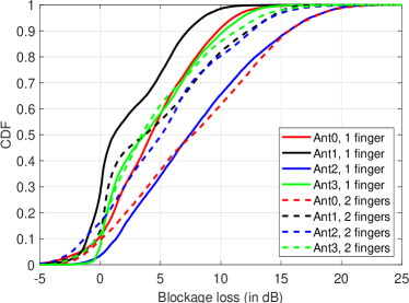
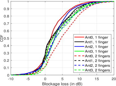
(a)	(b)

Figure 4: CDF of blockage losses with individual antenna elements for the (a) $0$ mm and (b) $1$ mm air gap scenarios with $1$ and $2$ fingers on the antenna module.

TABLE II: Blockage Loss Statistics with Individual Antenna Elements

	0 mm air gap, 1 finger				0 mm air gap, 2 fingers
Antenna index ($\rightarrow$)	0	1	2	3	0	1	2	3
Mean (in dB)	4.3	2.5	7.5	4.5	7.6	4.7	5.1	4.6
Std. dev (in dB)	4.4	3.8	5.8	4.3	6.2	5.3	5.5	4.8
	1 mm air gap, 1 finger				1 mm air gap, 2 fingers
Antenna index ($\rightarrow$)	0	1	2	3	0	1	2	3
Mean (in dB)	2.2	2.8	3.0	3.5	5.3	3.2	3.8	4.3
Std. dev (in dB)	3.9	4.6	4.1	4.6	4.9	4.6	5.1	4.5

With these choices, Figs. 4(a) and (b) capture the cumulative distribution functions (CDFs) of losses with the individual antenna elements (that is, $G_{{\sf free},i}(\theta,\phi)-G_{{\sf blockage},i}(\theta,\phi)$ with $(\theta,\phi)\in{\sf RoI}_{i}$) for the $0$ mm and $1$ mm air gap cases considered here. In general, we note that the losses seen with two fingers are more than those seen in the one finger case. Also, the losses seen with the $1$ mm air gap are smaller than when the hand touches the antenna module ($0$ mm air gap). Both these observations are intuitive and obvious as two fingers obstruct more coverage than one finger, and the $1$ mm air gap allows creeping of electromagnetic waves and thus better energy reception than with fingers on the antenna module. These observations are also captured in Table II which reports the mean and standard deviation of blockage losses over ${\sf RoI}_{i}$ for the different antenna elements in these settings.

IV Impact of Beamforming on Blockage

IV-A Optimal/Infinite-Precision Beamforming

While the studies in Sec. III considered the amplitude distortions seen at an individual antenna element level (which are of broader interest in initial link acquisition [23, 22]), for peak performance, the $4\times 1$ array is used with analog beamforming. To understand the implications of blockage in a practical context, we first consider the optimal beamforming solution along the direction $(\theta,\phi)$ where $\bullet$ is used to denote $\bullet\in\{{\sf free},{\sf blockage}\}$ and ^⋆ denotes the complex conjugate operation. This solution is given as

$${\bf G}_{{\sf opt},\hskip 1.4457pt\bullet}(\theta,\phi)=\max_{w_{i}\hskip 1.4457pt:\hskip 1.4457pt\sum_{i}|w_{i}|^{2}\leq 1}10\cdot\log_{10}\left(\left|\sum_{i=1}^{N}w_{i}^{\star}E_{\bullet,\hskip 1.4457pti}(\theta,\phi)\right|^{2}\right)$$

which can be seen to be the maximum ratio combining (MRC) solution with

$$w_{i}\Big{|}_{\sf opt}=\frac{E_{\bullet,\hskip 1.4457pti}(\theta,\phi)}{\sqrt{\sum_{i=1}^{N}|E_{\bullet,\hskip 1.4457pti}(\theta,\phi)|^{2}}}$$

resulting in

$${\bf G}_{{\sf opt},\hskip 1.4457pt\bullet}(\theta,\phi)=10\cdot\log_{10}\left(\sum_{i=1}^{N}|E_{\bullet,\hskip 1.4457pti}(\theta,\phi)|^{2}\right).$$

It is important to note that the above solution requires infinite-precision phase and amplitude control (that is, an infinite number of beams in the codebook) and is hence not practical in implementations. In this context, the main purpose of this solution is only to benchmark the performance of more practical codebook-based schemes relative to an upper bound on performance.

Contour plots capturing the optimal beamforming gain over the sphere in Freespace and with one or two fingers in the $0$ mm air gap case are plotted in Figs. 5(a)-(c). These plots show that hand blockage can lead to significant performance degradation over a good part of the coverage area of the antenna module. To quantify these gains, the CDFs of the optimal beamforming gain are plotted for the different scenarios in Fig. 6(a) over the RoI of $(\theta,\phi)=\left(150^{\sf o},\hskip 1.4457pt360^{\sf o}\right)\times\left(0^{\sf o},\hskip 1.4457pt180^{\sf o}\right)$. The median beamforming gain in Freespace is $11.5$ dB, whereas in the $0$ mm air gap scenario, the median gains are $7.4$ dB and $5.6$ dB (one and two fingers). For the $1$ mm air gap scenario, the median gains are $8.0$ dB and $6.9$ dB, respectively. These numbers show that a $3.5$ to $6$ dB median loss is seen with blockage, consistent with trends on loose hand grips reported in [18]. To be precise about blockage losses, in Fig. 6(b), we compare ${\bf G}_{{\sf opt},\hskip 1.4457pt{\sf free}}(\theta,\phi)$ with ${\bf G}_{{\sf opt},\hskip 1.4457pt{\sf blockage}}(\theta,\phi)$ for the different blockage scenarios. From this plot, we observe a median loss of $3.3$ and $4.5$ dB for the $0$ mm air gap, and $2.7$ and $3.5$ dB for the $1$ mm air gap scenarios, respectively. The corresponding $90$-th percentile loss values are $8.1$, $11.6$, $7.1$ and $9.4$ dB. Losses decrease by $\approx 1$ dB from the $0$ mm to $1$ mm air gap, whereas losses increase by a similar amount for one to two fingers. These observations show that the hand can indeed substantially deteriorate the link performance relative to Freespace operation, requiring careful remediation.

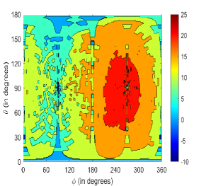
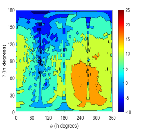
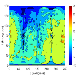
(a)	(b)	(c)
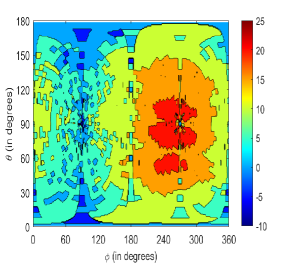
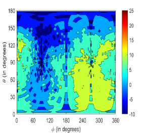
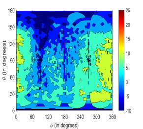
(d)	(e)	(f)

Figure 5: Gain with (a)-(c) optimal and (d)-(f) codebook-based beamforming over the sphere in Freespace, and $0$ mm air gap with one and two fingers, respectively.

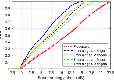
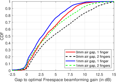
(a)	(b)
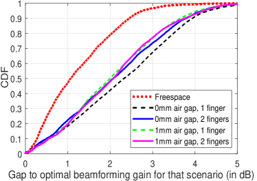
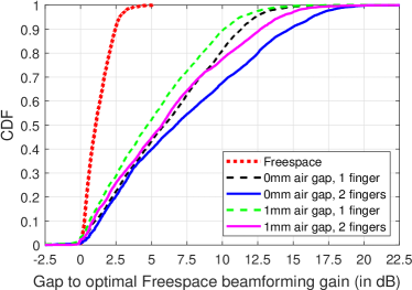
(c)	(d)

Figure 6: (a) CDF of optimal beamforming gain under all scenarios. (b) Loss in optimal beamforming gain under blockage scenarios relative to optimal beamforming in Freespace. Loss in codebook-based beamforming gain under Freespace and blockage scenarios relative to (c) the optimal scheme for that scenario and (d) optimal beamforming in Freespace.

IV-B Finite-Sized Beamforming Codebooks

In a practical deployment setting, beamforming is performed using a directional analog beamforming codebook (of size-$J$ where $J$ is chosen appropriately) denoted as ${\cal C}_{\sf dir}$ corresponding to a static set of beam weights where each beam weight steers energy in a fixed a priori determined direction. Note that this scheme is a low-complexity alternative to MRC and is a good scheme for sparse channels such as those seen at millimeter wave frequencies [23, 24, 25]. Let ${w}_{i,j},\hskip 1.4457pti=1,\cdots,N$ denote the unit-norm beam weights for the $j$-th directional beam ($j=1,\cdots,J$) with

$${\cal C}_{\sf dir}=\Big{\{}w_{i,j},\hskip 1.4457pti=1,\cdots,N,\hskip 1.4457ptj=1,\cdots,J\Big{\}}.$$

The realized gain with this directional codebook is given as

$${\bf G}_{{\sf cbk},\hskip 1.4457pt\bullet}(\theta,\phi)=\max_{j=1,\cdots,J}10\cdot\log_{10}\left(\left|\sum_{i=1}^{N}w_{i,j}^{\star}E_{\bullet,\hskip 1.4457pti}(\theta,\phi)\right|^{2}\right)$$

along the direction $(\theta,\phi)$.

It is typical to use $J=N$ for an array of $N$ antenna elements since this arrangement leads to an $\approx 2.5$ dB cross-over point between adjacent/neighboring beams over the coverage area of the antenna array. With $J=N=4$ here, we design beam weights to steer energy in fixed equi-spaced directions in beamspace. In Figs. 5(d)-(f), we illustrate the contour plot of the beamforming gain over the sphere with the codebook-based schemes showing a comparable performance with the optimal beamforming schemes. In Fig. 6(c), the performance of the scheme with size-$4$ codebooks is compared with the optimal beamforming scheme in that scenario. These plots show that in Freespace, the loss ranges from $1.1$ dB at the median to $2.5$ dB at the $90$-th percentile, which is in agreement with the design of a size-$N$ codebook for an $N\times 1$ array. On the other hand, the median loss in blockage scenarios (with the codebook relative to the optimal scheme) range from $2$ to $2.3$ dB, whereas the $90$-th percentile ranges from $3.7$ to $3.9$ dB suggesting that the directional codebook-based beamforming can suffer a significant performance degradation over the optimal scheme than in Freespace operation.

Also, the loss in performance with ${\cal C}_{\sf dir}$ over the optimal performance in Freespace is plotted in Fig. 6(d). These plots show that the median loss with a $1$ mm air gap are $4.7$ and $5.8$ dB (one and two fingers) matching up with numbers seen in prior works. When that $1$ mm air gap becomes $0$ mm, the median numbers increase to $5.9$ and $6.7$ dB — an increase of loss by $\approx 1$ dB. The corresponding $90$-th percentile loss numbers are $10.1$, $11.3$, $12.7$ and $14.7$ dB, which appears to be significant to warrant a dramatic loss in link performance. These observations motivate the need to improve performance over ${\cal C}_{\sf dir}$, which is the subject of the next section.

V Blockage Mitigation Via Non-Directional Codebooks

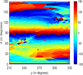
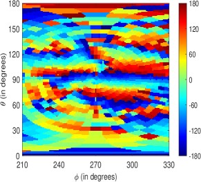
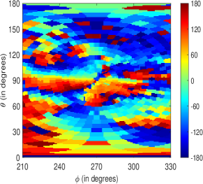
(a)	(b)	(c)

Figure 7: Phase response (a) with Freespace measurements and with $0$ mm air gap corresponding to (b) one and (c) two fingers.

V-A A Closer Look at the Impact of Blockage on Phases

Towards improving the performance of ${\cal C}_{\sf dir}$, we start with a more careful study of the true impact of blockage on the phases seen by the antenna elements. In Figs. 7(a)-(c), the phase response (denoted as $\angle{\Delta E_{\bullet}(\theta,\phi)}$) for Antenna 2 with respect to Antenna 1 is plotted for the Freespace case, $0$ mm air gap with one and two fingers, respectively (where $\bullet\in\{{\sf free},{\sf blockage}\}$). Note that

$$\angle{\Delta E_{\sf free}(\theta,\phi)} = \angle{E_{{\sf free},\hskip 1.4457pt2}(\theta,\phi)}-\angle{E_{{\sf free},\hskip 1.4457pt1}(\theta,\phi)}$$

$$\angle{\Delta E_{\sf blockage}(\theta,\phi)} = \angle{E_{{\sf blockage},\hskip 1.4457pt2}(\theta,\phi)}-\angle{E_{{\sf blockage},\hskip 1.4457pt1}(\theta,\phi)}.$$

From a visual perspective, the presence of the hand phantom leads to significant phase distortions captured as distinct color mixings within expected regions of contiguous phase behavior (from the Freespace plot in Fig. 7(a)). To quantitatively capture the extent of this phase mixing, we define the following metric:

$${\sf Measure}{\hskip 2.8903pt}{\sf of}{\hskip 2.8903pt}{\sf phase}{\hskip 2.8903pt}{\sf mixing}={\bf E}_{\theta,\phi}\Big{[}\left|\nabla_{\theta}\left\{\angle{\Delta E_{\bullet}(\theta,\phi)}\right\}\right|\Big{]}.$$

Since the $4\times 1$ array is placed on the Z axis, the phase response in the ideal scenario varies only over $\theta$ with no variations over $\phi$ motivating the above choice of the metric, which captures the average of the absolute directional gradient (direction of interest being $\theta$). In the practical case where measurements are made in Freespace, from Fig. 7(a), we observe that there are jumps in phases over $\theta$ (and significantly smaller jumps over $\phi$), which when averaged would lead to a small value for the phase mixing metric. On the other hand, if there is a considerable volatility (or spread) in phases as the hand phantom can induce, the corresponding values for the phase mixing metric can be large. Thus, a small value for the phase mixing metric captures a close to ideal phase response and a large value captures a significant phase distortion.

With this context, we compute the phase mixing metric from the measurement data to be $13.0^{\sf o}$, $21.2^{\sf o}$ and $20.6^{\sf o}$ for the Freespace, $0$ mm air gap cases with one and two fingers, respectively. These observations show that a significant phase distortion is induced by the hand phantom with the fingers leading to deviation in phase response from Freespace behavior. While Antenna 2’s (relative to Antenna 1) phase behavior is presented here, the conclusion seems to be similar across all the other antenna pairs as well as across polarizations (not presented here due to space constraints). In general, the presence of the fingers of the hand on top of/near the antenna module leads to angle- and antenna element-dependent amplitude and phase distortions due to multiple sets of reflections of the radiation from the antenna element (radiator) by the indentations of the fingers. These distortions can be modeled as:

$$E_{{\sf blockage},\hskip 1.4457pti}(\theta,\phi)=E_{{\sf free},\hskip 1.4457pti}(\theta,\phi)\cdot\underbrace{A_{i}(\theta,\phi)e^{jP_{i}(\theta,\phi)}}_{\sf Distortion},\hskip 3.61371pti=1,\cdots,N$$

where $A_{i}(\theta,\phi)$ and $P_{i}(\theta,\phi)$ capture the distortions illustrated in Figs. 3 and 7, respectively.

The intuitive explanation behind the poor performance of ${\cal C}_{\sf dir}$ relative to the optimal scheme in Sec. IV-B is the following. Note that ${\cal C}_{\sf dir}$ consists of beam weights that steer beams towards fixed directions in beamspace. Directional beams are well understood to produce a low-rank approximation of the dominant eigen-modes of a sparse channel such as those encountered at millimeter wave frequencies [23, 25]. On the other hand, closely approximating the eigen-modes of the channel (and in particular, the optimal MRC solution) requires the use of a linear combination of beams steered along different directions and the use of high-resolution phase shifter and gain controls at each antenna element [24]. Furthermore, the optimal beamforming weights in the blockage scenario are given as

$$w_{i}\Big{|}_{\sf opt}=\frac{E_{{\sf free},\hskip 1.4457pti}(\theta,\phi)\cdot A_{i}(\theta,\phi)e^{jP_{i}(\theta,\phi)}}{\sqrt{\sum_{i=1}^{N}|E_{{\sf free},\hskip 1.4457pti}(\theta,\phi)|^{2}\cdot A_{i}(\theta,\phi)^{2}}},$$

which requires knowledge of the distortion. A static codebook of steered beams (e.g., ${\cal C}_{\sf dir}$) cannot realize such beam weights leading to its relatively high loss, as illustrated in Fig. 6(c). Note that the entries of ${\cal C}_{\sf dir}$ are quantized with a $B=5$ bit phase shifter (with a $11.25^{\sf o}$ quantization spread). Thus, the phase mixing by the hand can lead to destructive interference with the entries of ${\cal C}_{\sf dir}$. The above observations motivate that any effective blockage mitigation strategy has to address the amplitude and phase distortions.

Given that the amplitude and phase distortions are a function of the user’s hand properties, hand grip, material property variations over frequency, antenna array properties (e.g., array size and geometry, impact of housing), etc., mitigating these distortions by learning them appears difficult. With a lack of ability in learning them, these distortions essentially appear to be random from the perspective of beamforming. Thus, we consider a robust approach and design an enhancement to ${\cal C}_{\sf dir}$ captured by a set of phase shifters and/or amplitude controls that can sample the space of all possible phases and/or amplitudes with low overhead. This design is described next.

V-B Proposed Non-Directional Codebook Design

For this, we start by considering a $B$-bit phase shifter that can (ideally) produce $2^{B}$ phase possibilities:

$$\phi_{k}=\frac{2\pi\cdot k}{2^{B}},\hskip 3.61371ptk=0,\cdots,2^{B}-1.$$

We then consider a codebook enhancement ${\cal C}_{\sf enh,\hskip 1.4457ptphase}$ of size-$(2^{B})^{N-1}$ where

$${\cal C}_{\sf enh,\hskip 1.4457ptphase}=\Big{\{}u_{k_{2},\hskip 1.4457pt\cdots,\hskip 1.4457ptk_{N}},\hskip 3.61371ptk_{\ell}=0,\cdots,2^{B}-1,\hskip 3.61371pt\ell=2,\cdots,N\Big{\}},$$

with each set of beam weights being of the functional form:

$$u_{k_{2},\hskip 1.4457pt\cdots,\hskip 1.4457ptk_{N}}=\frac{1}{\sqrt{N}}\cdot\left[\begin{array}[]{c}1\\ e^{j\phi_{k_{2}}}\\ \vdots\\ e^{j\phi_{k_{N}}}\end{array}\right].$$ (5)

Note that only the relative phases of the antenna elements with respect to the first antenna matters and thus without loss in generality, we can set the first phase term ($\phi_{k_{1}}$) to be $0$ for all the codebook entries. The basic motivation behind the structure of ${\cal C}_{\sf enh,\hskip 1.4457ptphase}$ is to sample each antenna element with a $B$-bit phase shifter with the best set of beam weights from ${\cal C}_{\sf enh,\hskip 1.4457ptphase}$ being the closest de-randomizer of the phase distortions induced by the hand. The effective role of the de-randomizer is to incorporate the impact of the hand distortions in the beam weights used, thereby matching the beam weights to the effective channel response as well as the hand effects and thus improving the realized array gains.

Since blockage induces both amplitude and phase distortions, the optimal beam weights for this scenario need to incorporate a search over both amplitudes and phases. Unlike phases with a limited range of $2\pi$, approximating the amplitude information can lead to a quick increase in codebook size and therefore the overhead associated with learning these beam weights. Thus, to overcome this complexity, we consider a beam training procedure with $N$ beams, each of which excites only one of the $N$ antenna elements at any instant. Let ${\sf S}_{i},\hskip 1.4457pti=1,\cdots,N$ denote the estimated signal strength with the $i$-th beam that excites the $i$-th antenna. This beam training is performed after the introduction of hand blockage so that ${\sf S}_{i}$ can be estimated with the presence of the hand.

Based on these signal strengths, we consider a codebook enhancement where

$${\cal C}_{\sf enh,\hskip 1.4457ptphase,\hskip 1.4457ptamp}=\Big{\{}v_{k_{2},\hskip 1.4457pt\cdots,\hskip 1.4457ptk_{N}},\hskip 3.61371ptk_{\ell}=0,\cdots,2^{B}-1,\hskip 3.61371pt\ell=2,\cdots,N\Big{\}},$$

with each set of beam weights being of the functional form:

$$v_{k_{2},\hskip 1.4457pt\cdots,\hskip 1.4457ptk_{N}}=\frac{1}{\sqrt{\sum_{i=1}^{N}{\sf S}_{i}}}\cdot\left[\begin{array}[]{c}\sqrt{{\sf S}_{1}}\\ \sqrt{{\sf S}_{2}}\cdot e^{j\phi_{k_{2}}}\\ \vdots\\ \sqrt{{\sf S}_{N}}\cdot e^{j\phi_{k_{N}}}\end{array}\right].$$ (10)

As before, we can set $\phi_{k_{1}}=0$. In the above structure, instead of searching for the amplitude of the $i$-th antenna element, we approximate it by the normalized square root of the signal strength based on selecting the $i$-th antenna element. Note that instead of using the true/estimated ${\sf S}_{i}$, if we used ${\sf S}_{i}=\frac{1}{N}$ for all $i$, then $v_{k_{2},\hskip 1.4457pt\cdots,\hskip 1.4457ptk_{N}}$ reduces to $u_{k_{2},\hskip 1.4457pt\cdots,\hskip 1.4457ptk_{N}}$.

V-C Theoretical Performance Comparisons

We now compare the performance of ${\cal C}_{\sf enh,\hskip 1.4457ptphase,\hskip 1.4457ptamp}$ with ${\cal C}_{\sf enh,\hskip 1.4457ptphase}$ and ${\cal C}_{\sf dir}$ in the blockage setting. For this, we consider a channel matrix ${\sf H}$ corresponding to $L$ dominant clusters over which beamformed transmissions are used at both the base station (with $M$ antenna elements) and UE (with $N$ antenna elements) ends. Let this $N\times M$ channel matrix ${\sf H}$ be given as [26]

$${\sf H}=\sum_{\ell=1}^{L}\alpha_{\ell}\cdot{\bf E}_{\sf blockage}(\theta_{{\sf R},\hskip 1.4457pt\ell},\phi_{{\sf R},\hskip 1.4457pt\ell}){\bf a}_{\sf T}(\theta_{{\sf T},\hskip 1.4457pt\ell},\phi_{{\sf T},\hskip 1.4457pt\ell})^{H}$$ (11)

where $\alpha_{\ell}$, $\theta_{{\sf R},\hskip 1.4457pt\ell}$, $\phi_{{\sf R},\hskip 1.4457pt\ell}$, $\theta_{{\sf T},\hskip 1.4457pt\ell}$ and $\phi_{{\sf T},\hskip 1.4457pt\ell}$ denote the complex gain, elevation and azimuth angles at the UE and base station ends, respectively, and $(\cdot)^{H}$ denotes the complex conjugate Hermitian operation. The $N\times 1$ vector ${\bf E}_{\sf blockage}(\theta,\phi)$ captures the electric field vector at the UE end under blockage setting and is given as

$${\bf E}_{\sf blockage}(\theta,\phi)=\left[\begin{array}[]{c}E_{{\sf blockage},\hskip 1.4457pt1}(\theta,\phi)\\ \vdots\\ E_{{\sf blockage},\hskip 1.4457ptN}(\theta,\phi)\end{array}\right],$$ (15)

with the $M\times 1$ vector ${\bf a}_{\sf T}(\theta,\phi)$ capturing the array steering vector at the base station side over the $(\theta,\phi)$ angle pair. Note that the model considered in (11) is the same as the Saleh-Valenzuela model [26], popularly used in studies of millimeter wave systems, with the difference being that the array steering vector at the UE end is replaced with the electric field vector to capture the impact of the UE housing and material properties and polarization mismatches/impairments on the steering vector.

We assume that the base station and the UE beamform along unit-norm vectors ${\bf f}$ (of size $M\times 1$) and ${\bf g}$ (of size $N\times 1$) to lead to the following scalar input-output equation model:

$$\widehat{\sf s}=\sqrt{\rho}\cdot{\bf g}^{H}{\sf H}{\bf f}{\sf s}+{\bf g}^{H}{\bf n}$$

with ${\sf s}$ being the scalar input from a certain constellation, $\widehat{\sf s}$ being its estimate, ${\bf n}\in{\cal CN}({\bf 0},{\bf I}_{N})$ being the additive white Gaussian noise and $\rho$ being the transmit power. With this setup, the received ${\sf SNR}$ is given as

$${\sf SNR}_{\sf rx}=\frac{\rho\cdot|{\bf g}^{H}{\sf H}{\bf f}|^{2}}{{\bf E}\left[|{\bf g}^{H}{\bf n}|^{2}\right]}=\frac{\rho\cdot|{\bf g}^{H}{\sf H}{\bf f}|^{2}}{{\bf g}^{H}\cdot{\bf I}_{N}\cdot{\bf g}}=\rho\cdot|{\bf g}^{H}{\sf H}{\bf f}|^{2}.$$

Without loss in generality, we assume that $\rho=1$ and $|\alpha_{1}|\geq\cdots\geq|\alpha_{L}|$. Thus, the angles corresponding to the dominant cluster are $\theta_{{\sf R},\hskip 1.4457pt1}$, $\phi_{{\sf R},\hskip 1.4457pt1}$, $\theta_{{\sf T},\hskip 1.4457pt1}$ and $\phi_{{\sf T},\hskip 1.4457pt1}$. We make the practical assumption of the use of a large antenna array at the base station end with beamforming over a narrow beamwidth to the dominant cluster in the channel. That is,

$$|{\bf a}_{\sf T}(\theta_{{\sf T},\hskip 1.4457pt1},\phi_{{\sf T},\hskip 1.4457pt1})^{H}{\bf f}| \approx 1,\hskip 3.61371pt{\sf and}$$

$${\bf a}_{\sf T}(\theta_{{\sf T},\hskip 1.4457pt\ell},\phi_{{\sf T},\hskip 1.4457pt\ell})^{H}{\bf f} \approx 0,\hskip 3.61371pt\ell=2,\cdots,L.$$

With these assumptions, we have the following simplification:

$${\sf SNR}_{\sf rx}\approx|\alpha_{1}|^{2}\cdot\left|{\bf g}^{H}{\bf E}_{\sf blockage}(\theta_{{\sf R},\hskip 1.4457pt1},\phi_{{\sf R},\hskip 1.4457pt1})\right|^{2}\triangleq\widetilde{\sf SNR}_{\sf rx}.$$

We first discuss the performance realized with ${\cal C}_{\sf dir}$ under blockage. For this, we note that

$$\frac{\max\limits_{{\bf g}\hskip 1.4457pt\in\hskip 1.4457pt{\cal C}_{\sf dir}}\widetilde{\sf SNR}_{\sf rx}}{|\alpha_{1}|^{2}}=\frac{1}{N}\cdot\max_{j}\left|\sum_{i}|E_{{\sf free},\hskip 1.4457pti}(\theta_{{\sf R},\hskip 1.4457pt1},\phi_{{\sf R},\hskip 1.4457pt1})|\cdot A_{i}(\theta_{{\sf R},\hskip 1.4457pt1},\phi_{{\sf R},\hskip 1.4457pt1})\cdot e^{j\psi_{i}}\right|^{2}$$

where $w_{ij}=\frac{1}{\sqrt{N}}\cdot e^{j\angle{w_{ij}}}$ and we have defined

$$\psi_{i}=\angle{E_{{\sf free},\hskip 1.4457pti}(\theta_{{\sf R},\hskip 1.4457pt1},\phi_{{\sf R},\hskip 1.4457pt1})}+P_{i}(\theta_{{\sf R},\hskip 1.4457pt1},\phi_{{\sf R},\hskip 1.4457pt1})-\angle{w_{ij}},\hskip 3.61371pti=1,\cdots,N.$$

While the performance seen with ${\cal C}_{\sf dir}$ is a function of how blockage impacts the antenna response, it is important to note that $\angle{w_{ij}}$ is determined based on beam steering requirements in Freespace (alone). Thus, the $\psi_{i}$’s have no constraints on their ranges and $\psi_{i}\in[0,2\pi)$ in general. As a result, some hand holdings can lead to constructive addition of the antenna responses, whereas some hand holdings can lead to destructive addition of the antenna responses. In this sense, ${\cal C}_{\sf dir}$ does not lead to a robust performance with blockage with the worst-case blockage performance (in terms of the phases $\{P_{i}\}$) being given as

$$\min\limits_{\{P_{i}\}}\frac{\max\limits_{{\bf g}\hskip 1.4457pt\in\hskip 1.4457pt{\cal C}_{\sf dir}}\widetilde{\sf SNR}_{\sf rx}}{|\alpha_{1}|^{2}} = \min\limits_{\{P_{i}\}}\frac{1}{N}\cdot\max_{j}\left|\sum_{i}|E_{{\sf free},\hskip 1.4457pti}(\theta_{{\sf R},\hskip 1.4457pt1},\phi_{{\sf R},\hskip 1.4457pt1})|\cdot A_{i}(\theta_{{\sf R},\hskip 1.4457pt1},\phi_{{\sf R},\hskip 1.4457pt1})\cdot e^{j\psi_{i}}\right|^{2}$$

$$= \min\limits_{a_{i}\hskip 1.4457pt\in\hskip 1.4457pt\pm 1}\frac{1}{N}\cdot\max_{j}\left|\sum_{i}|E_{{\sf free},\hskip 1.4457pti}(\theta_{{\sf R},\hskip 1.4457pt1},\phi_{{\sf R},\hskip 1.4457pt1})|\cdot A_{i}(\theta_{{\sf R},\hskip 1.4457pt1},\phi_{{\sf R},\hskip 1.4457pt1})\cdot a_{i}\right|^{2}.$$

While the precise choice of $\{a_{i}\}$ that minimizes the received ${\sf SNR}$ is a function of the relative antenna strengths seen with blockage across the antenna array, when multiple antenna elements see comparable signal strengths with blockage, if their relative phases $\{P_{i}\}$ are not aligned up perfectly in relation to $\angle{w_{ij}}$, destructive interference can lead to poor performance with ${\cal C}_{\sf dir}$. In this context, by choosing the phases $\{\phi_{k_{i}}\}$ for ${\cal C}_{\sf enh,\hskip 1.4457ptphase,\hskip 1.4457ptamp}$ and ${\cal C}_{\sf enh,\hskip 1.4457ptphase}$ appropriately, the range of $\psi_{i}$ can be restricted (or reduced) and received ${\sf SNR}$ performance can be improved over that of ${\cal C}_{\sf dir}$. Of these two codebook choices, based on classical tradeoffs between equal gain combining and MRC solutions, it is intuitively expected that amplitude and phase control can improve performance over phase-only control [27]. In particular, let the improvement in received ${\sf SNR}$ using ${\cal C}_{\sf enh,\hskip 1.4457ptphase,\hskip 1.4457ptamp}$ over ${\cal C}_{\sf enh,\hskip 1.4457ptphase}$ be defined as

$$\widetilde{\Delta}{\sf SNR}_{\sf rx}\triangleq\frac{\Delta{\sf SNR}_{\sf rx}}{|\alpha_{1}|^{2}}=\frac{\max\limits_{{\bf g}\hskip 1.4457pt\in\hskip 1.4457pt{\cal C}_{\sf enh,\hskip 1.4457ptphase,\hskip 1.4457ptamp}}\widetilde{\sf SNR}_{\sf rx}-\max\limits_{{\bf g}\hskip 1.4457pt\in\hskip 1.4457pt{\cal C}_{\sf enh,\hskip 1.4457ptphase}}\widetilde{\sf SNR}_{\sf rx}}{|\alpha_{1}|^{2}}.$$

We now quantify $\widetilde{\Delta}{\sf SNR}_{\sf rx}$ in Theorem 1.

Theorem 1

In the high-SNR setting and assuming $B\geq 1$, $\widetilde{\Delta}{\sf SNR}_{\sf rx}$ is bounded as

$$\widetilde{\Delta}{\sf SNR}_{\sf rx} \geq N\cdot{\sf Var}_{\sf blockage}\cdot\cos^{2}\left(\frac{\pi}{2^{B}}\right)-\frac{2\sin^{2}\left(\frac{\pi}{2^{B}}\right)}{N}\cdot\left(\sum|E_{{\sf blockage},\hskip 1.4457pti}(\theta_{{\sf R},\hskip 1.4457pt1},\phi_{{\sf R},\hskip 1.4457pt1})|\right)^{2}$$

$$\triangleq \Delta{\sf SNR}_{\sf rx,\hskip 1.4457ptLB}$$

where ${\sf Var}_{\sf blockage}$ denotes the variance of the electric field vector under blockage and is given as

$${\sf Var}_{\sf blockage} = \frac{\sum_{i}|E_{{\sf blockage},\hskip 1.4457pti}(\theta_{{\sf R},\hskip 1.4457pt1},\phi_{{\sf R},\hskip 1.4457pt1})|^{2}}{N}-\left(\frac{\sum_{i}|E_{{\sf blockage},\hskip 1.4457pti}(\theta_{{\sf R},\hskip 1.4457pt1},\phi_{{\sf R},\hskip 1.4457pt1})|}{N}\right)^{2}.$$

Proof:

See Appendix -A. ∎

There are a number of parameters that impact $\Delta{\sf SNR}_{\sf rx,\hskip 1.4457ptLB}$ as defined in Theorem 1. Clearly, $\Delta{\sf SNR}_{\sf rx,\hskip 1.4457ptLB}$ is maximized as $\cos^{2}\left(\frac{\pi}{2^{B}}\right)$ approaches $1$ (or as $B$ increases). Further, for a choice of $B$ and $\{E_{{\sf blockage},\hskip 1.4457pti}(\theta_{{\sf R},\hskip 1.4457pt1},\phi_{{\sf R},\hskip 1.4457pt1})\}$ such that $\sum_{i}|E_{{\sf blockage},\hskip 1.4457pti}(\theta_{{\sf R},\hskip 1.4457pt1},\phi_{{\sf R},\hskip 1.4457pt1})|$ is held constant, $\Delta{\sf SNR}_{\sf rx,\hskip 1.4457ptLB}$ is maximized when ${\sf Var}_{\sf blockage}$ reaches its largest value. Note that ${\sf Var}_{\sf blockage}$ reaches its smallest and largest values when $|E_{{\sf blockage},\hskip 1.4457pti}(\theta_{{\sf R},\hskip 1.4457pt1},\phi_{{\sf R},\hskip 1.4457pt1})|$ are equal for all $i$ and only one of the $|E_{{\sf blockage},\hskip 1.4457pti}(\theta_{{\sf R},\hskip 1.4457pt1},\phi_{{\sf R},\hskip 1.4457pt1})|$’s dominate all the other, respectively. In other words, $\Delta{\sf SNR}_{\sf rx,\hskip 1.4457ptLB}$ is the largest when the amplitudes seen with blockage lead to the widest disparity across antenna elements and in this setting, we have

$$\Delta{\sf SNR}_{\sf rx,\hskip 1.4457ptLB}=\max_{i}|E_{{\sf blockage},\hskip 1.4457pti}(\theta_{{\sf R},\hskip 1.4457pt1},\phi_{{\sf R},\hskip 1.4457pt1})|^{2}\cdot\left[\cos^{2}\left(\frac{\pi}{2^{B}}\right)\cdot\left(1-\frac{1}{N}\right)-\frac{2}{N}\sin^{2}\left(\frac{\pi}{2^{B}}\right)\right].$$

The above intuition is not surprising (in hindsight) since ${\cal C}_{\sf enh,\hskip 1.4457ptphase,\hskip 1.4457ptamp}$ performs amplitude control over ${\cal C}_{\sf enh,\hskip 1.4457ptphase}$, and amplitude control in MRC is necessitated and is useful when the amplitude response across antenna elements affects the antenna elements differently. Thus, when the hand distorts the effective response across the antenna elements in an unequal manner, the efficacy of ${\cal C}_{\sf enh,\hskip 1.4457ptphase,\hskip 1.4457ptamp}$ over ${\cal C}_{\sf enh,\hskip 1.4457ptphase}$ or ${\cal C}_{\sf dir}$ is amplified, with more unequal the array response, the better the efficacy.

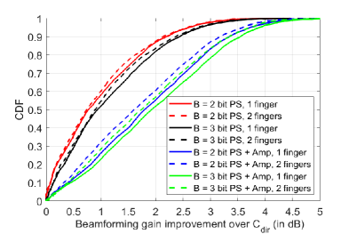
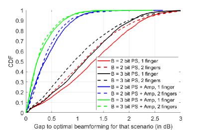
(a)	(b)

Figure 8: (a) Performance improvement over ${\cal C}_{\sf dir}$ for different codebook enhancement schemes. (b) Gap to optimal beamforming with proposed codebook enhancement schemes.

V-D Numerical Studies

Depending on the angle of arrival of the dominant cluster at the UE end, Fig. 3 shows that the amplitude response across antenna elements can be either comparable or not comparable leading to good performance with ${\cal C}_{\sf enh,\hskip 1.4457ptphase}$ and no need for ${\cal C}_{\sf enh,\hskip 1.4457ptphase,\hskip 1.4457ptamp}$, or the need for ${\cal C}_{\sf enh,\hskip 1.4457ptphase,\hskip 1.4457ptamp}$ to improve blockage performance. To quantify the performance of de-randomizing the phases and/or amplitudes, we consider four schemes for numerical evaluation in the $0$ mm air gap case with one and two fingers. For the first scheme, with $B=2$, note that the phases of each antenna element are of the form $\{1,j,-1,-j\}$ and with $N=4$, we consider a ${\cal C}_{\sf enh,\hskip 1.4457ptphase}$ of size-$64$ ($=(2^{B})^{N-1}=(2^{2})^{3}$). For the second scheme, in the $B=3$ case, the size of ${\cal C}_{\sf enh,\hskip 1.4457ptphase}$ is $512$ ($=(2^{3})^{3}$). In addition to these two phase shifter-only selection schemes, we also consider the amplitude and phase shifter selection scheme with $B=2$ and $B=3$ as the third and fourth schemes, respectively.

For these four schemes, Fig. 8(a) plots the beamforming gain improvement with the codebook enhancements over ${\cal C}_{\sf dir}$ for the $0$ mm air gap case with one and two fingers. From these plots, we observe the median, $80$-th and $90$-th percentile performance improvement of $0.7$, $1.7$ and $2.1$ dB for the first scheme (substantial numbers in practical settings) suggesting that the fingers of the hand do actually randomize the phases of different antenna elements which ${\cal C}_{\sf enh,\hskip 1.4457ptphase}$ can de-randomize. Increasing $B$ in the phase shifter selection approach only leads to a marginal performance improvement (comparable improvement of $0.9$, $1.9$ and $2.4$ dB) suggesting that most of the gains with phase shifter selection are captured with the $B=2$ bit phase shifter choice. On the other hand, addition of the signal strength to mirror an MRC-type solution can lead to significant gains ($1.6$ dB at the median and $3.2$ dB at the $90$-th percentile). Similar numbers for $B=3$ phase and amplitude control over phase-only control are $1.7$ dB gain at median and $3.3$ dB at the $90$-th percentile, again reinforcing that $B=2$ is sufficient. Thus, it is important to consider a hand blockage mitigation strategy that mirrors and accounts for the signal strength and phase variations seen across the antenna array commensurate with the hand position.

To complement this study, Fig. 8(b) shows the gap in performance between these schemes and the optimal MRC scheme (which can be viewed as the “unrecovered gain”). The median, $80$-th and $90$-th percentile values of unrecovered gains with the $B=2$ bit phase shifter based search are $1.1$, $1.8$ and $2.2$ dB suggesting the possibility of better schemes. With the third scheme, the corresponding numbers are $0.35$, $0.65$ and $0.85$ dB. Further reduction in these unrecovered gains could be possible with a larger size of ${\cal C}_{\sf enh,\hskip 1.4457ptphase}$ or ${\cal C}_{\sf enh,\hskip 1.4457ptphase,\hskip 1.4457ptamp}$ (such as with $B=3$). However, the increase in the search space produces diminishing gains and the search complexity can also lead to latencies associated with beam management, which can in turn translate to increased power consumption and thermal overheads. Thus, it is of broad interest in understanding the optimal size and structure of codebook enhancements, which could be of interest in future work.

VI Concluding Remarks

The scope of this work has been on understanding the implications of hand blockage at millimeter wave frequencies. We first report chamber measurements performed with a commercial grade millimeter wave modem and a commercial grade hand phantom at $28$ GHz which captured the complete electric field information (array response) in Freespace and with different blockage settings. The blockage settings correspond to the use of a hand phantom with different spacings to the antenna module of interest and one or two fingers obstructing the antenna elements. These studies showed that a loose hand grip-based loss estimates capture the observed blockage losses. Further, the use of two fingers leads to more losses than one finger and the presence of an air gap between the hand phantom and the antenna module reduces the losses.

We then quantified the performance loss between the use of a static directional beam steering codebook of size-$4$ for the $4\times 1$ array (typical practical deployment numbers) relative to the optimal MRC beamforming scheme. These loss estimates showed that while the static codebook is a good codebook for Freespace considerations, it performs relatively poorly with hand blockage. This is because the fingers of the hand induce random phase and amplitude distortions due to multiple reflections from different parts of the hand, which a static codebook cannot take advantage of. In this context, we introduced a codebook enhancement of a quantized set of phase shifter combinations which do not carry a directional structure and simply quantize the space of all possible phase combinations. We showed that this codebook enhancement, both theoretically as well as with measurement data, can lead to significant performance improvement over the static beam steering codebook suggesting that the randomization of phases by the presence of the hand can be de-randomized by the enhanced codebook.

Future work on understanding the limits of such codebook enhancements taking into account latency with a pre-determined set of phase excitations, beam search complexity, power and thermal constraints would be of immense practical importance. Maximum permissible exposure (MPE) constraints and the need to perform regulation-driven beam characterization can lead to significant complexity as the size of the codebook enhancement increases (e.g., $B$ of the phase shifter). Thus, decoupling the uplink and downlink beams at the UE side (breaking down beam correspondence [28]) and the tradeoffs associated with this breakdown are of broad interest. Implications of hand blockage on better antenna array design as well as at upper millimeter wave bands (e.g., $60$ GHz and beyond) are of interest. Extending these ideas to larger arrays commonly used in customer premises equipments, integrated access and backhaul nodes, intelligent reflecting surfaces, or base-stations where non-blockage issues such as fading still effectively induce the same type of amplitude and phase randomization effects [24] would also be of broader utility.

References

- [1] V. Raghavan, R. A. Motos, M. A. Tassoudji, Y-C. Ou, O. H. Koymen, and J. Li, “Hand blockage modeling and beamforming codebook mitigation strategies,” Proc. IEEE Intern. Conf. Commun., Montreal, Canada, pp. 1–6, June 2021.
- [2] A. Maltsev et al., “Channel models for 60 GHz WLAN systems, doc: IEEE 802.11-09/0334r8,” May 2010, Available: [Online]. https://mentor.ieee.org/802.11/documents.
- [3] 3GPP TR 38.901 V14.3.0 (2017-12), “Technical Specification Group Radio Access Network; Study on Channel Model for Frequencies from 0.5 to 100 GHz (Rel. 14),” Dec. 2017.
- [4] G. R. MacCartney, Jr. and T. S. Rappaport, “A flexible millimeter-wave channel sounder with absolute timing,” IEEE Journ. Sel. Areas in Commun., vol. 35, no. 6, pp. 1402–1418, June 2017.
- [5] G. R. MacCartney, Jr., T. S. Rappaport, and S. Rangan, “Rapid fading due to human blockage in pedestrian crowds at 5G millimeter-wave frequencies,” Proc. IEEE Global Telecommun. Conf., Singapore, pp. 1–7, Dec. 2017.
- [6] K. Zhao, J. Helander, Z. Ying, D. Sjöberg, M. Gustafsson, and S. He, “mmWave phased array in mobile terminal for 5G mobile system with consideration of hand effect,” Proc. IEEE Veh. Tech. Conf. (Spring), Glasgow, Scotland, pp. 1–4, May 2015.
- [7] K. Zhao, J. Helander, D. Sjöberg, S. He, T. Bolin, and Z. Ying, “User body effect on phased array in user equipment for the 5G mmWave communication system,” IEEE Ant. and Wireless Propagat. Letters, vol. 16, pp. 864–867, 2017.
- [8] K. Zhao, C. Gustafson, Q. Liao, S. Zhang, T. Bolin, and Z. Ying, “Channel characteristics and user body effects in an outdoor urban scenario at 15 and 28 GHz,” IEEE Trans. Ant. Propagat., vol. 65, no. 12, pp. 6534–6548, Dec. 2017.
- [9] I. Syrytsin, S. Zhang, G. F. Pedersen, K. Zhao, T. Bolin, and Z. Ying, “Statistical investigation of the user effects on mobile terminal antennas for 5G applications,” IEEE Trans. Ant. Propagat., vol. 65, no. 12, pp. 6596–6605, Dec. 2017.
- [10] B. Yu, K. Yang, C. Sim, and G. Yang, “A novel 28 GHz beam steering array for 5G mobile device with metallic casing application,” IEEE Trans. Ant. Propagat., vol. 66, no. 1, pp. 462–466, Jan. 2018.
- [11] B. Xu, Z. Ying, L. Scialacqua, A. Scannavini, L. J. Foged, T. Bolin, K. Zhao, S. He, and M. Gustafsson, “Radiation performance analysis of 28 GHz antennas integrated in 5G mobile terminal housing,” IEEE Access, vol. 6, pp. 48088–48101, 2018.
- [12] M. Heino, C. Icheln, and K. Haneda, “Finger effect on 60 GHz user device antennas,” Proc. European Conf. Ant. Propagat., Davos, Switzerland, pp. 1–5, Apr. 2016.
- [13] M. Heino, C. Icheln, and K. Haneda, “Self-user shadowing effects of millimeter-wave mobile phone antennas in a browsing mode,” Proc. European Conf. Ant. Propagat., Krakow, Poland, pp. 1–5, Apr. 2019.
- [14] J. Hejselbæk, J. Ø. Nielsen, W. Fan, and G. F. Pedersen, “Measured 21.5 GHz indoor channels with user-held handset antenna array,” IEEE Trans. Ant. Propagat., vol. 65, no. 12, pp. 6574–6583, Dec. 2017.
- [15] I. Syrytsin, S. Zhang, and G. F. Pedersen, “User impact on phased and switch diversity arrays in 5G mobile terminals,” IEEE Access, vol. 6, pp. 1616–1623, 2018.
- [16] V. Raghavan, L. Akhoondzadeh-Asl, V. Podshivalov, J. Hulten, M. A. Tassoudji, O. H. Koymen, A. Sampath, and J. Li, “Statistical blockage modeling and robustness of beamforming in millimeter wave systems,” IEEE Trans. Microwave Theory and Tech., vol. 67, no. 7, pp. 3010–3024, July 2019.
- [17] V. Raghavan, V. Podshivalov, J. Hulten, M. A. Tassoudji, A. Sampath, O. H. Koymen, and J. Li, “Spatio-temporal impact of hand and body blockage for millimeter-wave user equipment design,” IEEE Commun. Magaz., vol. 56, no. 12, pp. 46–52, Dec. 2018.
- [18] V. Raghavan, S. Noimanivone, S-K. Rho, B. Farin, P. Connor, R. A. Motos, Y-C. Ou, K. Ravid, M. A. Tassoudji, O. H. Koymen, and J. Li, “Hand and body blockage measurements with form-factor user equipment at 28 GHz,” Submitted to IEEE Trans. Ant. Propagat., 2020, Available: Online. https://arxiv.org/abs/1912.03717.
- [19] SPEAG, “Hand phantoms,” Available: [Online]. https://speag.swiss/products/em-phantoms/phantoms.
- [20] S. Vyavahare, S. Teraiya, D. Panghal, and S. Kumar, “Fused deposition modelling: A review,” Rapid Prototyping Journ., vol. 26, no. 1, pp. 176–201, Jan. 2020.
-
[21]
Keysight Technologies,
“White paper on ‘OTA Test for Millimeter-Wave 5G NR Devices and
Systems’,”
2017,
Available: [Online].
https://www.keysight.com/upload/cmc_upload/All/5992-2600EN_10-5-17_CS.pdf. - [22] V. Raghavan, M-L. (Clara) Chi, M. A. Tassoudji, O. H. Koymen, and J. Li, “Antenna placement and performance tradeoffs with hand blockage in millimeter wave systems,” IEEE Trans. Commun., vol. 67, no. 4, pp. 3082–3096, Apr. 2019.
- [23] V. Raghavan, J. Cezanne, S. Subramanian, A. Sampath, and O. H. Koymen, “Beamforming tradeoffs for initial UE discovery in millimeter-wave MIMO systems,” IEEE Journ. Sel. Topics in Sig. Proc., vol. 10, no. 3, pp. 543–559, Apr. 2016.
- [24] V. Raghavan, S. Subramanian, J. Cezanne, and A. Sampath, “Directional beamforming for millimeter-wave MIMO systems,” Proc. IEEE Global Telecommun. Conf., San Diego, CA, pp. 1–7, Dec. 2015, Extended version, Available: Online. http://www.arxiv.org/abs/1601.02380.
- [25] V. Raghavan, A. Partyka, L. Akhoondzadeh-Asl, M. A. Tassoudji, O. H. Koymen, and J. Sanelli, “Millimeter wave channel measurements and implications for PHY layer design,” IEEE Trans. Ant. Propagat., vol. 65, no. 12, pp. 6521–6533, Dec. 2017.
- [26] A. A. M. Saleh and R. Valenzuela, “A statistical model for indoor multipath propagation,” IEEE Journ. Sel. Areas in Commun., vol. 5, no. 2, pp. 128–137, Feb. 1987.
- [27] D. J. Love and R. W. Heath, Jr., “Equal gain transmission in multiple-input multiple-output wireless systems,” IEEE Trans. Commun., vol. 51, no. 7, pp. 1102–1110, July 2003.
- [28] 3GPP TR 38.912 V14.1.0 (2017-08), “Technical Specification Group Radio Access Network; Study on New Radio (NR) access technology (Rel. 14),” Aug. 2017.