Joint Matrix Completion and Compressed Sensing for State Estimation in Low-observable Distribution System

Abstract

Limited measurement availability at the distribution grid presents challenges for state estimation and situational awareness. This paper combines the advantages of two sparsity-based state estimation approaches (matrix completion and compressive sensing) that have been proposed recently to address the challenge of unobservability. The proposed approach exploits both the low rank structure and a suitable transform domain representation to leverage the correlation structure of the spatio-temporal data matrix while incorporating the power-flow constraints of the distribution grid. Simulations are carried out on three phase unbalanced IEEE 37 test system to verify the effectiveness of the proposed approach. The performance results reveal - (1) the superiority over traditional matrix completion and (2) very low state estimation errors for high compression ratios representing very low observability.

I Introduction

Distribution grid operation is becoming more challenging due to an increase in the penetration of distributed energy resources. Instances of reverse power flow and undesired voltage rise has increased and will occur more frequently in the future. Therefore, state estimation (SE) is critical for the monitoring and control of a distribution grid. However, extending the conventional SE approaches for the distribution grid is difficult mainly because the system is highly unobservable at the grid edge. The estimation of the network states with only a limited number of measurements is a major challenge. Furthermore, the various characteristics of distribution grids such as low $X/R$ ratio [1], limited bandwidth capacity, unbalanced operation [2], and cyber-security issues hinders the successful adoption of conventional SE approaches in distribution grids.

Weighted least squares (WLS) estimation represents the conventional approach for distribution system state estimation (DSSE). To address the low-observability issue of distribution system, historical data based pseudo-measurements are used along-with the WLS approach. However, the inaccuracies in pseudo-measurements impacts the state estimation performance [3]. Data driven approaches proposed in [4] employ model-free structure to estimate the voltage states. However, these approaches still require large number of PMUs to be installed. Recently, sparsity-based approaches have been used for DSSE to address the challenge of unobservability. These approaches exploit the network structure to estimate the states at the current levels of measurement availability. These approaches neither require pseudo-measurements nor any extra metering devices. Compressive sensing (CS) based DSSE was one of the first sparsity-based solution proposed in [5]. This approach exploits the spatial and temporal sparsity of measurements in a linear transformation basis [6], [7]. Matrix completion (MC) [8] based DSSE is an another alternative to deal with limited system observability. This method leverages the standard matrix completion along-with the power-flow constraints to acknowledge the physical network constraints. A comparative analysis of these sparsity based approaches for DSSE along-with their robust formulation is presented in [9]. Authors in [10] proposes a Gaussian process based approach along-with matrix completion to deal with multi time-scale measurements in a smart distribution system.

In order to accurately estimate the states with high probability using the sparsity based approaches, the requirement of minimum number of measurements must be satisfied. In compressive sensing, the reconstruction of length $N$ states using $M$ measurements where $M\ll N$ is possible by exploiting the sparsity of states in a transformed basis. $K$-sparse states are recovered accurately using $M\geq cK\mbox{log}(N/K)$ i.i.d gaussian measurements [11]. In a matrix completion approach, the minimum number of measurements ($m$) required to recover the matrix of size $n_{1}\times n_{2}$ with high probability is $m\geq Cn^{1.2}r\mbox{log}n$ where $n=max(n_{1},n_{2})$ and $r$ is the rank of matrix [12]. These requirements restrict the application of sparsity based approaches for highly unobservable distribution system. Furthermore, in the matrix completion approach the minimization of nuclear norm requires solving a semi-definite program which becomes computationally inefficient for large matrices. An efficient alternating minimization algorithm is proposed in [13] that reformulates the matrix completion problem with time-series data.

This paper proposes two unique approaches to estimate the system states when availability of spatio-temporal measurements at the local control center is very limited. We consider a commonly occurring practical scenario where the sensors at specific spatial locations send data to the local center at a particular sampling rate. The first proposed approach estimates the states by performing matrix completion across space and compressive sensing across time using an alternating minimization approach. This formulation estimates the states in a single shot by exploiting the low rank property as well as temporal sparsity in the measurements while incorporating the power-flow constraints.

In the second approach, the compressive sensing and matrix completion are performed in two stages. In the first stage, the compressed measurements from a single sensor are recovered by exploiting the sparsity of the states in a linear transformation basis. In the second stage, matrix completion across the network is performed at individual time instants. The contributions of this paper are as follows:

• An efficient and unique state estimation formulation that combines matrix completion and compressive sensing based approaches in a single powerflow constrained optimization framework is proposed for the first time.

• The proposed approach exploits the low rank property and compactness of temporal data in the wavelet transform domain. We validate that both these property (low-rank and DCT compactness) hold true for practical data.

• The proposed algorithm effectively estimates the states with high fidelity in very low observability region. We demonstrate the performance of the algorithm for IEEE 37 unbalanced test system. Relative to the classical matrix completion approaches, the error performance of the proposed approach offer nearly 91% improvement at 10% of the fraction of available measurements.

II Background

Consider a power distribution grid with $|\mathcal{P}|$ three phase non-slack buses. Sensors are deployed throughout the grid but due to communication and other constraints, only a fraction of data is aggregated from these sensors and used for DSSE. This section first reviews the classic matrix completion and compressive sensing approaches for DSSE.

II-A Classic Matrix completion

In a classic matrix completion based approach for DSSE, a structured matrix $\mathbf{M}$ is formed such that each column represents a phase and each row represents a measurement associated with the phase of each bus. The matrix is given as,

$$[\Re(v_{i}),\Im(v_{i}),|v_{i}|,\Re(s_{i}),\Im(s_{i})]^{\intercal}$$ (1)

where, $s_{i}$ and $v_{i}$ represents the apparent power injection and voltages of the $i^{th}$ bus respectively. The term $\Re(\cdot)$ and $\Im(\cdot)$ represents the real and imaginary part of a complex variable respectively.

In a distribution system, the matrix $\mathbf{M}$ is partially observed. At the local control center, only a subset of the measurement matrix i.e. $P_{\Omega}(\mathbf{M})$ is available. The goal is to fill the missing entries in the matrix by exploiting the relationship among the raw measurements. Specifically, the missing elements of the matrix are filled by suitable low-rank approximation augmented with the power-flow constraints [9]. The corresponding optimization formulation is given as,

$$\mathbf{\hat{X}}=\underset{\mathbf{X}\in\mathbb{R}^{5\times|\mathcal{P}|}}{\text{\enspace argmin}}\enspace\|\mathbf{X}\|_{*}$$ (2)

subject to $$\|P_{\Omega}({\mathbf{M}})-P_{\Omega}(\mathbf{X})\|_{F}^{2}<\epsilon$$

$$\mathbf{v\approx B}\begin{bmatrix}\Re(\mathbf{s})\\ \Im(\mathbf{s})\end{bmatrix}+\mathbf{w},$$ (3)

$$\mathbf{|v|\approx C\mathbf{missing}}\begin{bmatrix}\Re(\mathbf{s})\\ \Im(\mathbf{s})\end{bmatrix}+\mathbf{|w|},$$ (4)

where, (3) and (4) captures the linearized power-flow constraints given in [14]. Here, the nuclear norm $\|\mathbf{X}\|_{*}=\sum_{i=1}^{r=min(5,|\mathcal{P}|)}\sigma_{i}(\mathbf{X})$ is the sum of the singular values of the matrix $\mathbf{X}$. While matrix completion exploits the spatial correlation by low rank approximation, it fails to capture the temporal correlation of the states. Another sparsity based approach that effectively captures spatial or temporal correlation is compressive sensing discussed in II.B.

II-B Classic compressive sensing

Compressive sensing based DSSE exploits the temporal or spatial sparsity of measurements or states in a linear transformation basis. Let the states $\mathbf{z}\in\mathbb{R}^{N}$ be compressible in a linear transformation basis such that,

$$\mathbf{z}=\mathbf{Da}$$ (5)

where a has at most $K$ $\ll$ $N$ significant coefficients i.e., z is $K$-sparse in sparsifying basis $\mathbf{D}$. Compressed measurements are achieved by taking $M\ll N$ random projections of $\mathbf{z}$,

$$\mathbf{h}=\mathbf{\Phi}\mathbf{z};\mathbf{h}\in\mathbb{R}^{M},\mathbf{\Phi}\in\mathbb{R}^{M\times N},$$ (6)

where, $\mathbf{\Phi}$ is a random measurement/projection matrix (e.g., matrix elements distributed as i.i.d. Gaussian random variable with mean $0$ and variance $1/M$ or Bernoulli random variables).

In spatial CS, the states $\mathbf{z}=[\Re(\mathbf{s}),\Im(\mathbf{s}),\tilde{\mathbf{v}}]^{\intercal}$ can be estimated by solving the following $l_{1}$ minimization problem

$$\mathbf{\hat{a}}= \underset{\mathbf{s}}{\text{\enspace min}}\enspace\|\mathbf{s}\|_{1}$$ (7)

$$\text{subject to}\enspace\mathbf{\|h-\Phi Ds\|_{2}^{2}}<\epsilon$$

$$\mathbf{v\approx B}\begin{bmatrix}\Re(\mathbf{s})\\ \Im(\mathbf{s})\end{bmatrix}+\mathbf{w},$$ (8)

The recovered states $\mathbf{\hat{z}}$ are given as $\mathbf{\hat{z}}=\mathbf{D}\mathbf{\hat{a}}$. Here, $\|\mathbf{s}\|_{1}$ represents the $l_{1}$ norm and $\mathbf{B}$, $\mathbf{w}$ are as defined earlier. The compression of the states $\mathbf{z}$ is indicated by the compressed measurement ratio (CMR) given as $CMR=\frac{M}{N}$. In spatial CS, in order to construct the projection matrix $\mathbf{\Phi}$, the elements of $\mathbf{z}$ should be known apriori. However, it may not be practical to construct this matrix. Another form of CS captures the temporal sparsity of each states $\mathbf{z}$ whose optimization formulation is similar to (7) except the powerflow constraints (8). Thus, it is makes sense to incorporate matrix completion in space and compressive sensing in time to exploit the sparsity of the states. Jointly incorporating both of these approaches would aid in accurately recovering the states in low-observable conditions.

III Proposed Approach

In this section, we have proposed two approaches to jointly estimate the states using matrix completion and compressive sensing based DSSE techniques.

III-A Joint MC-CS approach

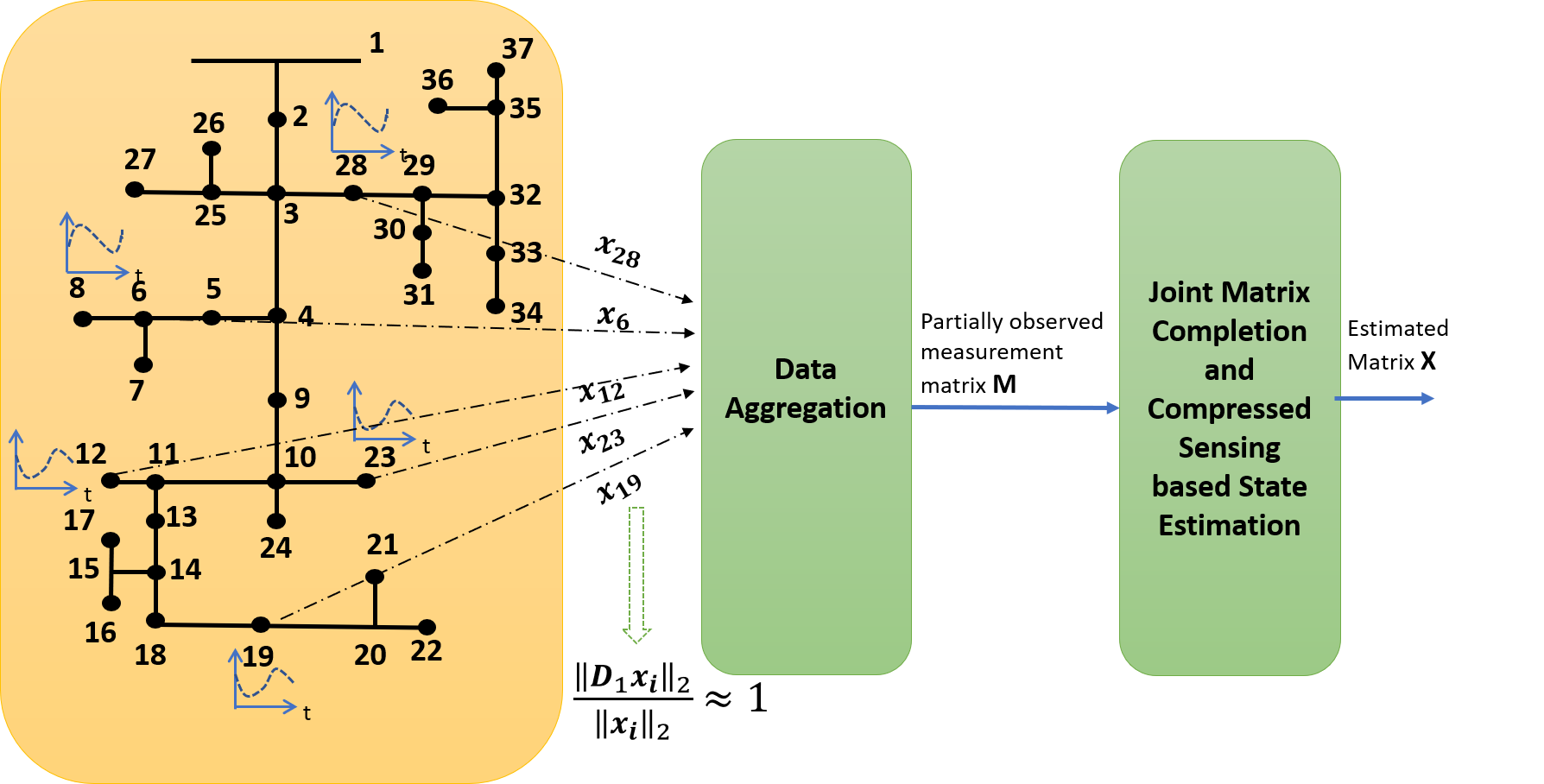
Figure 1: Framework of the Joint MC-CS approach

The framework of the joint MC-CS approach is shown in Fig.1. Assume the sensors located at a subset of buses send data to the local control center at time $t=1,2,...,T$ at a predefined sampling rate. Let $\mathbf{M}^{t}$ denote the measurement matrix at time $t$ whose structure is given in (1). A block matrix $\mathbf{M}$ is constructed as,

$$\mathbf{M}=[\mathbf{M}^{1};\mathbf{M}^{2};...,\mathbf{M}^{T}]\in\mathbb{R}^{m\times n}$$ (9)

Here, $m=5T$ and $n=|\mathcal{P}|$. The linearized powerflow constraints from (3) and (4) at time $t=1,..,T$ can be written as,

$$\mathbf{y\approx Ap+b}$$

$$\text{where}:\mathbf{y}=[\Re(\mathbf{v}^{1}),\Im(\mathbf{v}^{1}),|\mathbf{v}^{1}|,...,\Re(\mathbf{v}^{T}),\Im(\mathbf{v}^{T}),|\mathbf{v}^{T}|]^{\intercal},$$

$$\mathbf{A}=\begin{bmatrix}\mathbf{B_{1}}&\mathbf{B_{2}}&\mathbf{0}&\cdots&\mathbf{0}&\mathbf{0}\\ \mathbf{B_{3}}&\mathbf{B_{4}}&\mathbf{0}&\cdots&\mathbf{0}&\mathbf{0}\\ \mathbf{C_{1}}&\mathbf{C_{2}}&\mathbf{0}&\cdots&\mathbf{0}&\mathbf{0}\\ \vdots&\vdots&\vdots&\ddots&\mathbf{0}&\mathbf{0}\\ \mathbf{0}&\mathbf{0}&\mathbf{0}&\cdots&\mathbf{B_{1}}&\mathbf{B_{2}}\\ \mathbf{0}&\mathbf{0}&\mathbf{0}&\cdots&\mathbf{B_{3}}&\mathbf{B_{4}}\\ \mathbf{0}&\mathbf{0}&\mathbf{0}&\cdots&\mathbf{C_{1}}&\mathbf{C_{2}}\\ \end{bmatrix},$$

$$\mathbf{p}=[\Re(\mathbf{s}^{1})^{\intercal}\enspace\Im(\mathbf{s}^{1})^{\intercal}...\enspace\Re(\mathbf{s}^{T})^{\intercal}\enspace\Im(\mathbf{s}^{T})^{\intercal}]^{\intercal}$$

$$\text{and}\enspace\mathbf{b}=[\Re(\mathbf{w})^{\intercal},\Im(\mathbf{w})^{\intercal},|\mathbf{w}|^{\intercal}...\Re(\mathbf{w})^{\intercal},\Im(\mathbf{w})^{\intercal},|\mathbf{w}|^{\intercal}]^{\intercal}$$

where, the term $[\mathbf{B_{1}\enspace B_{2}}]=\Re(\mathbf{B})$, $[\mathbf{B_{3}\enspace B_{4}}]=\Im(\mathbf{B})$ and $[\mathbf{C_{1}\enspace C_{2}}]=\mathbf{C}$.

It is important to note that the rows/columns of the matrix $\mathbf{M}$ is observed to exhibit low rank feature and discrete cosine transform (DCT) compactness properties as discussed next.

III-A1 Low rank property

The columns of the matrix $\mathbf{M}$ are dependent on each other as there exists spatial correlation between different locations in a power grid. Furthermore, the physics of power-flow relates the different measurements. Hence, $\mathbf{M}$ possess low-rank property which can be evaluated by calculating the SVD of the matrix as,

$$\mathbf{M=U\Sigma V^{T}}$$ (10)

where the matrix $\mathbf{U}$ $\in$ $\mathbb{R}^{m\times m}$, $\mathbf{V}\in\mathbb{R}^{n\times n}$ and $\mathbf{\Sigma}\in\mathbb{R}^{m\times n}$ containing $p=min(m,n)$ singular values arranged in descending order ($\sigma_{1}>\sigma_{2}>...>\sigma_{p}$). For our experiments involving practical data from IEEE 37 bus test system, it can be inferred that the largest 5 singular values occupy about 99.9% of the energy confirming the low-rank property of the measurement matrix. This property has also been confirmed by other prior efforts on matrix completion [8].

III-A2 DCT compactness analysis

In a distribution network, the loads are observed to be slowly changing over time. The temporal data in the matrix $\mathbf{M}$ represented by $\mathbf{x}_{i}$ is observed to exhibit sparsity in a linear transformation basis [5]. Discrete cosine transform (DCT) enables to represent the data in a fewer coefficients. The DCT matrix $\mathbf{D}$ = ’$\{d(k,n)\}$’ of dimension $T\times T$ as defined in [15] can be split as,

$$\mathbf{D}=\begin{bmatrix}\mathbf{D}_{1}\\ \mathbf{D}_{2}\end{bmatrix}$$

where $\mathbf{D}_{1}$ consists of first ${}^{\prime}j^{\prime}$ rows of $\mathbf{D}$ and $\mathbf{D}_{2}$ consists of last ${}^{\prime}T-j^{\prime}$ rows. To exhibit temporal sparsity for the timeseries data $\mathbf{x}_{i}$, only few DCT coefficients will capture most of the energy i.e.,

$$\frac{\|\mathbf{D}_{1}\mathbf{x}_{i}\|_{2}}{\|\mathbf{x}_{i}\|_{2}}\approx 1,\enspace\frac{\|\mathbf{D}_{2}\mathbf{x}_{i}\|_{2}}{\|\mathbf{x}_{i}\|_{2}}\approx 0$$

This property can be observed from the practical time-series data from IEEE 37 bus test system where 1-2 DCT coefficients occupy 99% of the energy, thus proving the temporal data in matrix $\mathbf{M}$ is compact. However, due to limited system observability, only limited entries of the matrix $\mathbf{M}$ are observed. In order to recover the complete matrix, the low-rank feature property, DCT compactness and the linearized power-flow constraints are exploited in an integrated optimization formulation corresponding to,

$$\underset{\mathbf{X}}{\text{\enspace min}}\enspace\|\mathbf{X}\|_{*}+\lambda_{1}\|P_{\Omega}(\mathbf{X})-P_{\Omega}(\mathbf{M})\|_{F}^{2}+\nu\|\mathbf{y-(Ap+b)}\|_{2}^{2}+$$ (11)

$$\lambda_{2}\|\mathbf{s}\|_{2}$$

$$\textrm{s.t.}\quad\mathbf{y}=[a_{1}^{\intercal}\mathbf{X}\enspace a_{2}^{\intercal}\mathbf{X}\enspace...\enspace a_{3T-2}^{\intercal}\mathbf{X}\enspace a_{3T-1}^{\intercal}\mathbf{X}\enspace a_{3T}^{\intercal}\mathbf{X}]^{\intercal},$$

$$\mathbf{p}=[c_{1}^{\intercal}\mathbf{X}\enspace c_{2}^{\intercal}\mathbf{X}\enspace...\enspace c_{2T-1}^{\intercal}\mathbf{X}\enspace c_{2T}^{\intercal}\mathbf{X}]^{\intercal},$$

$$\mathbf{s}=\begin{bmatrix}\mathbf{D}_{2}\enspace(e_{4}^{\intercal}\enspace reshape(\mathbf{X}(:,1),[5,T]))^{\intercal}\\ \mathbf{D}_{2}\enspace(e_{5}^{\intercal}\enspace reshape(\mathbf{X}(:,1),[5,T]))^{\intercal}\\ \mathbf{D}_{2}\enspace(e_{1}^{\intercal}\enspace reshape(\mathbf{X}(:,1),[5,T]))^{\intercal}\\ \vdots\\ \mathbf{D}_{2}\enspace(e_{1}^{\intercal}\enspace reshape(\mathbf{X}(:,n),[5,T]))^{\intercal}\\ \end{bmatrix}$$

where, $m=5T$, $n=|\mathcal{P}|$, $\mathbf{X}\in\mathbb{R}^{m\times n}$, $\mathbf{y}\in\mathbb{R}^{\frac{3}{5}mn}$, $\mathbf{p}\in\mathbb{R}^{\frac{2}{5}mn}$
Here, $a_{3(t-1)+i}=e_{5(t-1)+i}$ and $c_{2(t-1)+i}=e_{5(t-1)+3+i}$ are the standard basis vectors in $\mathbb{R}^{m},$ $e_{1}$, $e_{4}$ and $e_{5}$ are the standard basis vectors in $\mathbb{R}^{5}$. The parameters $\lambda_{1}\geq 0$, $\nu\geq 0$, $\lambda_{2}\geq 0$ are the tuning parameters.
The matrix $\mathbf{X}$ can be factorized into two matrices $\mathbf{U}$ and $\mathbf{V}$. The nuclear norm of $\mathbf{X}$ can be expressed by the Frobenius norm of matrix $\mathbf{U}$ and $\mathbf{V}$ given as,

$${\|\mathbf{X}\|_{*}}= \underset{\mathbf{U},\mathbf{V}}{\text{\enspace min}}\enspace\|\mathbf{U}\|^{2}_{F}+\|\mathbf{V}\|^{2}_{F}$$ (12)

$$\text{subject to}\enspace\mathbf{X=UV}$$

Substituting (12) in (11), we obtain the following optimization problem,

$$\underset{\mathbf{U,V}}{\text{min}}\enspace\|\mathbf{U}\|^{2}_{F}+\|\mathbf{V}\|^{2}_{F}+\lambda_{1}\|P_{\Omega}(\mathbf{UV})-P_{\Omega}(\mathbf{M)}\|_{F}^{2}+$$ (13)

$$\nu\|f_{1}(\mathbf{UV})-(Af_{2}(\mathbf{UV})+\mathbf{b})\|_{2}^{2}+\lambda_{2}\|f_{3}(\mathbf{UV})\|_{2}$$

$$\textrm{s.t.}\quad f_{1}(\mathbf{UV})=[a_{1}^{\intercal}\mathbf{X}\enspace a_{2}^{\intercal}\mathbf{X}\enspace...\enspace a_{3T-2}^{\intercal}\mathbf{X}\enspace a_{3T-1}^{\intercal}\mathbf{X}\enspace a_{3T}^{\intercal}\mathbf{X}]^{\intercal},$$

$$f_{2}(\mathbf{UV})=[c_{1}^{\intercal}\mathbf{X}\enspace c_{2}^{\intercal}\mathbf{X}\enspace...\enspace c_{2T-1}^{\intercal}\mathbf{X}\enspace c_{2T}^{\intercal}\mathbf{X}]^{\intercal},$$

$$f_{3}(\mathbf{UV})=\begin{bmatrix}\mathbf{D}_{2}\enspace(e_{4}^{\intercal}\enspace reshape(\mathbf{X}(:,1),[5,T]))^{\intercal}\\ \mathbf{D}_{2}\enspace(e_{5}^{\intercal}\enspace reshape(\mathbf{X}(:,1),[5,T]))^{\intercal}\\ \mathbf{D}_{2}\enspace(e_{1}^{\intercal}\enspace reshape(\mathbf{X}(:,1),[5,T]))^{\intercal}\\ \vdots\\ \mathbf{D}_{2}\enspace(e_{1}^{\intercal}\enspace reshape(\mathbf{X}(:,n),[5,T]))^{\intercal}\\ \end{bmatrix}$$

$$\mathbf{X=UV}$$

The matrix completion formulation in (13) is a non-convex problem. But using alternating minimization algorithm [13], the problem becomes convex when either $\mathbf{U}$ or $\mathbf{V}$ is fixed. This algorithm updates the variables $\mathbf{U}$ and $\mathbf{V}$ at each iteration $k$ in an alternating fashion while fixing the other factor. The update rules are given by the following update equations as, [3] U^(k) ∥ U∥^2_F + λ_1 ∥ P_Ω(UV^(k-1)) - P_Ω(M)∥_F ^2 + ν ∥ f_1(UV^(k-1)) - (A f_2(UV^(k-1)) + b) ∥_2^2 + λ_2 ∥ f_3(UV^(k-1))∥_2 [2] V^(k) ∥ V∥^2_F + λ_1 ∥ P_Ω(U^kV)- P_Ω(M)∥_F ^2 + ν ∥ f_1(U^kV) - (A f_2(U^kV) + b) ∥_2^2 + λ_2 ∥ f_3(U^kV)∥_2 The alternating minimization approach for the proposed approach is given in Algorithm 1.

III-B CS-MC Approach

The joint MC-CS approach proposed in section III.A directly incorporates the raw information from each of the sensors at a particular bus for state estimation. However, due to the network bandwidth limitation, it may not be practical to collect all the temporal measurements. Furthermore, as stated earlier, to solve (9) involving large matrices can be computationally inefficient. Therefore, we propose a state estimation approach that alleviates these drawbacks.

The framework of the CS-MC approach is shown in Fig.2. Assume the measurements collected from each buses is $\mathbf{\Phi}\mathbf{x}$ where $\mathbf{\Phi}\mathbf{x}\ll$ $\mathbf{x}$. The recovery of the states is performed in two stages. Firstly, the incomplete temporal measurements are recovered by compressive sensing using (7). It should be noted that no power-flow constraints are used at this stage. Once the estimates of all the temporal measurements are obtained, the second stage consists of recovering the spatial states by classic matrix completion based state estimation using (2). The state estimation is performed separately at each time steps along-with the power-flow constraints in (3) and (4).

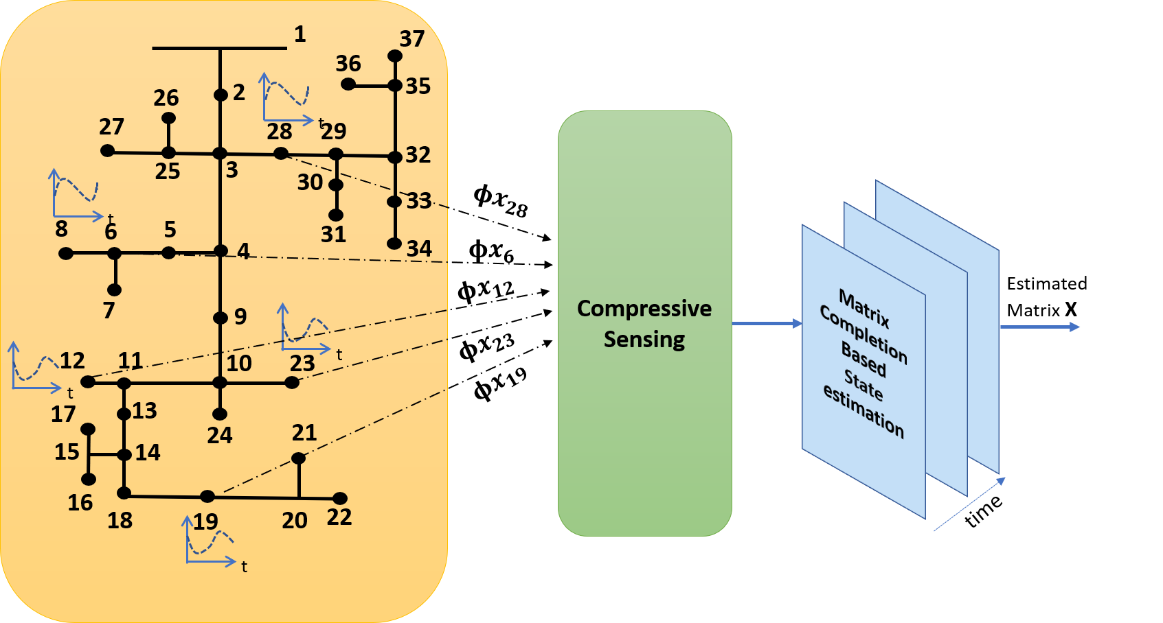
Figure 2: Framework of the CS-MC approach

Input: Measurement matrix $\mathbf{M}$, Set of known indices $\Omega$, DCT matrix $\mathbf{D}$, system model $\mathbf{A}$, $\mathbf{b}$, number of iterations $N$.

initialization: Compute the SVD of the matrix $\mathbf{M=U\Sigma V^{T}}$, set $\mathbf{V}^{(0)}=\mathbf{\Sigma}^{0.5}\mathbf{V}$

1:  for $k=1,..,N$ do

2:     Solve (13)

3:     Solve (13)

4:  end for

5:  return $\mathbf{X}=\mathbf{U}^{(N)}\mathbf{V}^{(N)}$

Algorithm 1 Alternating minimization Algorithm for matrix completion across space and compressive sensing across time

IV Computational Complexity

In this section, the computational complexity of the proposed approaches for a matrix $\mathbf{X}\in\mathcal{R}^{5T\times|\mathcal{P}|}$ is discussed. In the joint MC-CS approach, in order to solve the power-flow constraints, $\mathcal{O}(|\mathcal{P}|^{3}T^{3})$ computations are required at each iteration. In a classic MC approach, the matrix $\mathbf{X}\in\mathcal{R}^{5\times|\mathcal{P}|}$ is estimated separately for each time $T$. Denoting $m$ and $n$ as the rows and columns of $\mathbf{X}$, the main computation is involved in calculation of the SVD of the matrix which is $\mathcal{O}(mn\cdot\mbox{min}({m,n}))$ along-with the power-flow constraints $\mathcal{O}(n^{3})$ at each time. Hence, the overall worst case computational complexity is $\mathcal{O}(|\mathcal{P}|^{3}T)$. The CS-MC approach performs CS for each temporal state and classic matrix completion in the next step. CS requires $\mathcal{O}(T\cdot k\cdot\mbox{min}(T,k))$ computations where $T$ denotes the time and $k$ as constraints. The overall worst case complexity in both the steps is $\mathcal{O}(|\mathcal{P}|^{3}T)$. This illustrates that the proposed joint MC-CS approach is computationally expensive as compared to the conventional matrix completion as well as the CS-MC approach.

V Simulation Results and Discussion

In this section, the efficacy of the proposed formulation is demonstrated on the IEEE 37 unbalanced three phase test system. We characterize the performance of power and voltage magnitude recovery using the mean absolute percentage error (MAPE) metric and the voltage angle recovery using mean integrated absolute error (MIAE) metric [9]. For simulation, we consider a matrix that includes 8 time steps and whose entries are randomly available representing different fractions of available data (FAD). The compression of the temporal measurements in the CS-MC approach is indicated by CMR as defined earlier. Fig. 3 shows the recovery performance of power (active and reactive) using the two proposed approaches. Fig.4 -5 shows the comparative performance of the proposed formulation with the classic MC in the recovery of voltage magnitude and voltage angle states respectively. It can be inferred that the proposed joint MC-CS approach as well as the CS-MC approach outperforms the classic matrix completion at all FADs. The performance is superior especially in the low observability region. This is due to the fact that this approach exploits both the spatial correlation as well as temporal correlation of the states. The joint MC-CS approach, although computationally expensive, is superior than CS-MC approach. This is due to the fact that raw measurements are used for estimating the states rather than the compressed measurements. The recovery of states in CS-MC approach also depends on the CMR of the temporal measurements. The error in the recovery performance increases as the CMR is decreased. Fig. 3-5 shows the performance of CS-MC at 40% and 80% CMR.

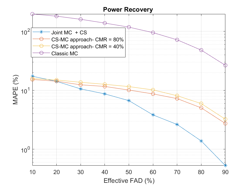
Figure 3: Power recovery at different FADs

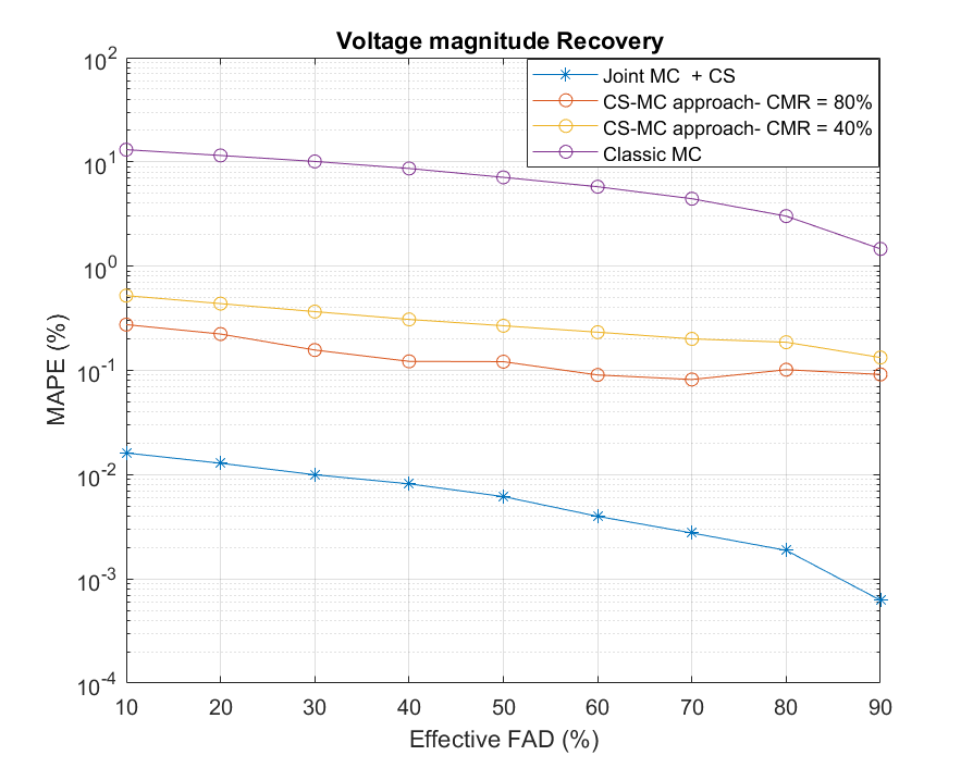
Figure 4: Voltage magnitude recovery at different FADs

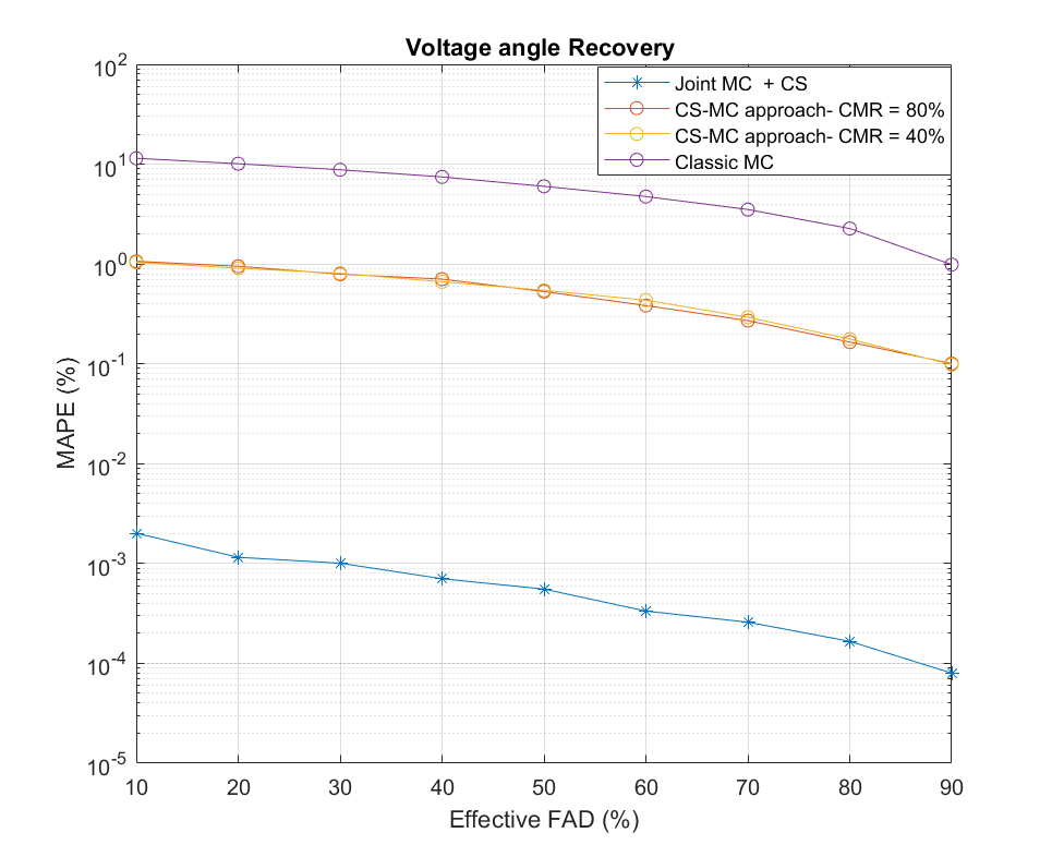
Figure 5: Voltage angle recovery at different FADs

VI Conclusion

This paper presents an efficient joint matrix completion and compressive sensing approach to perform DSSE. The proposed approach employs an alternating minimization approach to estimate an incomplete spatio-temporal matrix. The efficacy of the proposed approach was demonstrated using the IEEE 37 bus test system. It can be inferred from the simulation results that the proposed approach has a superior performance relative to classic matrix completion and provides lower state estimation errors at high compression ratios.

References

- [1] K. Dehghanpour, Z. Wang, J. Wang, Y. Yuan, and F. Bu, “A survey on state estimation techniques and challenges in smart distribution systems,” IEEE Transactions on Smart Grid, vol. 10, no. 2, pp. 2312–2322, 2018.
- [2] B. Hayes and M. Prodanovic, “State estimation techniques for electric power distribution systems,” in 2014 European Modelling Symposium. IEEE, 2014, pp. 303–308.
- [3] K. A. Clements, “The impact of pseudo-measurements on state estimator accuracy,” in 2011 IEEE Power and Energy Society General Meeting. IEEE, 2011, pp. 1–4.
- [4] M. Pertl, K. Heussen, O. Gehrke, and M. Rezkalla, “Voltage estimation in active distribution grids using neural networks,” in 2016 IEEE Power and Energy Society General Meeting (PESGM). IEEE, 2016, pp. 1–5.
- [5] S. S. Alam, B. Natarajan, and A. Pahwa, “Distribution grid state estimation from compressed measurements,” IEEE Transactions on Smart Grid, vol. 5, no. 4, pp. 1631–1642, 2014.
- [6] A. Joshi, L. Das, B. Natarajan, and B. Srinivasan, “A framework for efficient information aggregation in smart grid,” IEEE Transactions on Industrial Informatics, vol. 15, no. 4, pp. 2233–2243, 2018.
- [7] H. S. Karimi and B. Natarajan, “Compressive sensing based state estimation for three phase unbalanced distribution grid,” in GLOBECOM 2017-2017 IEEE Global Communications Conference. IEEE, 2017, pp. 1–6.
- [8] P. L. Donti, Y. Liu, A. J. Schmitt, A. Bernstein, R. Yang, and Y. Zhang, “Matrix completion for low-observability voltage estimation,” IEEE Transactions on Smart Grid, 2019.
- [9] S. Dahale, H. S. Karimi, K. Lai, and B. Natarajan, “Sparsity based approaches for distribution grid state estimation - a comparative study,” IEEE Access, vol. 8, pp. 198 317–198 327, 2020.
- [10] S. Dahale and B. Natarajan, “Multi time-scale imputation aided state estimation in distribution system,” arXiv preprint arXiv:2011.10738, 2020.
- [11] R. G. Baraniuk, “Compressive sensing [lecture notes],” IEEE signal processing magazine, vol. 24, no. 4, pp. 118–121, 2007.
- [12] E. J. Candès and B. Recht, “Exact matrix completion via convex optimization,” Foundations of Computational mathematics, vol. 9, no. 6, p. 717, 2009.
- [13] Y. Liu, A. Sagan, A. Bernstein, R. Yang, X. Zhou, and Y. Zhang, “Matrix completion using alternating minimization for distribution system state estimation,” in 2020 IEEE International Conference on Communications, Control, and Computing Technologies for Smart Grids (SmartGridComm). IEEE, 2020, pp. 1–6.
- [14] A. Bernstein and E. Dall’Anese, “Linear power-flow models in multiphase distribution networks,” in 2017 IEEE PES Innovative Smart Grid Technologies Conference Europe (ISGT-Europe). IEEE, 2017, pp. 1–6.
- [15] A. K. Jain, Fundamentals of digital image processing. Prentice-Hall, Inc., 1989.