ViT-V-Net: Vision Transformer for Unsupervised Volumetric Medical Image Registration

Abstract

In the last decade, convolutional neural networks (ConvNets) have dominated and achieved state-of-the-art performances in a variety medical imaging applications. However, the performances of ConvNets are still limited by lacking the understanding of long-range spatial relations in an image. The recently proposed Vision Transformer (ViT) for image classification uses a purely self-attention-based model that learns long-range spatial relations to focus on the relevant parts of an image. Nevertheless, ViT emphasizes the low-resolution features because of the consecutive downsamplings, result in a lack of detailed localization information, making it unsuitable for image registration. Recently, several ViT-based image segmentation methods have been combined with ConvNets to improve the recovery of detailed localization information. Inspired by them, we present ViT-V-Net, which bridges ViT and ConvNet to provide volumetric medical image registration. The experimental results presented here demonstrate that the proposed architecture achieves superior performance to several top-performing registration methods. Our implementation is available at https://bit.ly/3bWDynR.

1 Introduction

Deformable image registration (DIR) is fundamental for many medical image analysis tasks. It functions by of establishing spatial correspondences between points in a pair of fixed and moving images through a spatially varying deformation model. Traditionally, DIR can be performed by solving an optimization problem that maximizes the image similarity between the deformed moving and fixed images while enforcing smoothness constraints on the deformation field [Beg et al.(2005)Beg, Miller, Trouvé, and Younes, Avants et al.(2008)Avants, Epstein, Grossman, and Gee, Vercauteren et al.(2009)Vercauteren, Pennec, Perchant, and Ayache]. However, such optimization problems need to be solved for each pair of images, making those methods computationally expensive and slow in practice. Since recently, ConvNets-based registration methods [de Vos et al.(2017), Balakrishnan et al.(2018)Balakrishnan, Zhao, Sabuncu, Guttag, and Dalca, Sokooti et al.(2017), Chen et al.(2020)Chen, Li, Du, and Frey] have become a major focus of attention due to their fast computation time after training while achieving comparable accuracy to state-of-the-art methods.

Despite ConvNets’ promising performance, ConvNet architectures generally have limitations in modeling explicit long-range spatial relations (i.e., relations between two voxels that are far away from each other) present in an image due to the intrinsic locality of convolution operations [Chen et al.(2021)]. Many works have been proposed to overcoming this limitation, e.g. U-Net [Ronneberger et al.(2015)Ronneberger, Fischer, and Brox] (or V-Net [Milletari et al.(2016)Milletari, Navab, and Ahmadi]), atrous convolution (i.e, dilated convolution) [Yu and Koltun(2015)], and self-attention [Vaswani et al.(2017)]. Recently, there has been an increasing interest in developing self-attention-based architectures due to their great success in natural language processing. Methods like non-local networks [Wang et al.(2018)Wang, Girshick, Gupta, and He], detection transformer (DETR) [Carion et al.(2020)], and Axial-deeplab [Wang et al.(2020)] have exhibited superior performance in computer vision tasks. Dosovitskiy et al. [Dosovitskiy et al.(2020)] proposed Vision Transformer (ViT), a first purely self-attention-based network, and achieved state-of-the-art performance in image recognition. Subsequent to this progress, TransUnet [Chen et al.(2021)] was developed on the basis of a pre-trained ViT for 2-dimensional (2D) medical image segmentation. However, medical imaging modalities generally produce volumetric images (i.e., 3D images), and 2D images do not fully exploit the spatial correspondences obtained from 3D volumes. Therefore, developing 3D methods is more desirable in medical image registration. In this work, we present the first study to investigate the usage of ViT for volumetric medical image registration. We propose ViT-V-Net that employs a hybrid ConvNet-Transformer architecture for self-supervised volumetric image registration. In this method, the ViT was applied to high-level features of moving and fixed images, which required the network to learn long-distance relationships between points in images. Long skip connections between encoder and decoder stages were used to retain the flow of localization information. The experimental results demonstrated that a simple swapping of the network architecture of VoxelMorph with Vit-V-Net could produce superior performance to both VoxelMorph and conventional registration methods.

fig_arc

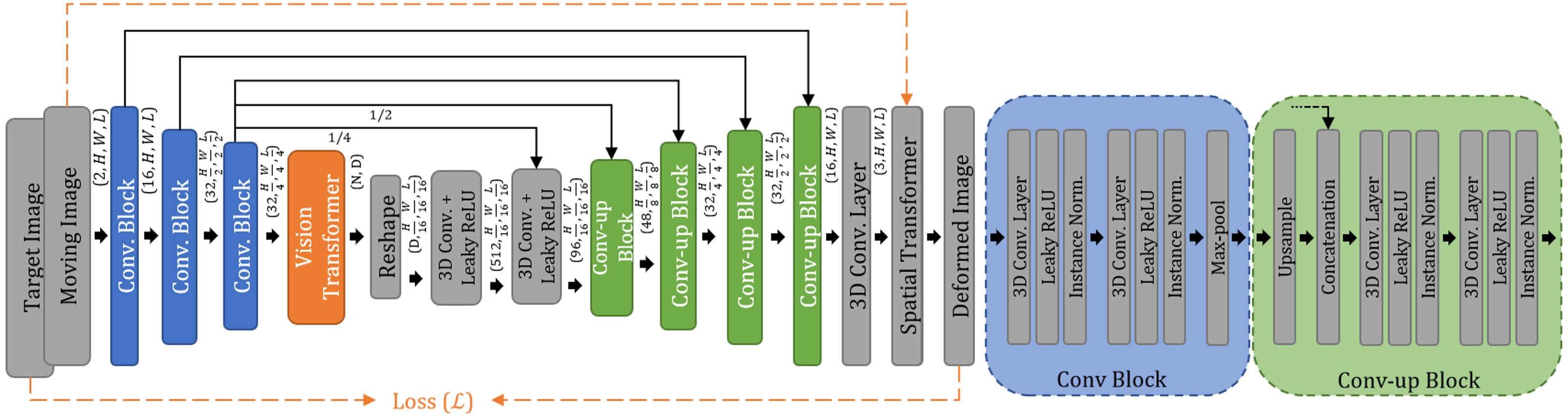
Figure 1: Method overview and network architecture of ViT-V-Net.

2 Methods

Let $f\in\mathbb{R}^{H\times W\times L}$ and $m\in\mathbb{R}^{H\times W\times L}$ be fixed and moving image volumes. We assume that $f$ and $m$ are single-channel grayscale images, and they are affinely aligned. Our goal is to predict a transformation function $\mathbf{\phi}$ that warps $m$ (i.e., $m\circ\mathbf{\phi}$) to $f$, where $\mathbf{\phi}=Id+\mathbf{u}$, $\mathbf{u}$ denotes a flow field of displacement vectors, and $Id$ denotes the identity. Fig. LABEL:fig_arc presents an overview of our method. First, the deep neural network ($g_{\theta}$) generates $\mathbf{u}$, for the given image pair $f$ and $m$, using a set of parameters $\theta$ (i.e., $\mathbf{u}=g_{\theta}(f,m)$). Then, the warping (i.e., $m\circ\mathbf{\phi}$) is performed via a spatial transformation function [Jaderberg et al.(2015)Jaderberg, Simonyan, Zisserman, and Kavukcuoglu]. During network training, image similarity between $m\circ\mathbf{\phi}$ and $f$ is compared, and the loss is backpropagated into the network.

ViT-V-Net Architecture Naive application of ViT to full-resolution volumetric images leads to large computational complexity. Here, instead of feeding full-resolution images directly into the ViT, the images (i.e., $f$ and $m$) were first encoded into high-level feature representations via a series of convolutional layers and max-poolings (blue boxes in Fig. LABEL:fig_arc). In the ViT (orange box), the high-level features were then separated into $N$ vectorized $P^{3}\times C$ patches, where $N=\frac{HWL}{P^{3}}$, $P$ denotes the patch size, and $C$ is the channel size. Next, the patches were mapped to a latent $D$-dimensional space using a trainable linear projection (i.e., patch embedding). Learnable position embeddings are then added to the patch embeddings to retain positional information of the patches [Dosovitskiy et al.(2020)]. Next, the resulting patches were fed into the Transformer encoder, which consisted of 12 alternating layers of Multihead Self-Attention (MSA) and Multi-Layer Perceptron (MLP) blocks [Vaswani et al.(2017)] (see Appendix A for details of ViT). Finally, the output from ViT was reshaped and then decoded using a V-Net style decoder. Notice that long skip connections between the encoder and decoder were also used. The network’s final output is a dense displacement field, which was then used in the spatial transformer for warping $m$.

Loss Functions The image similarity measurement used in this study was mean squared error (MSE), along with a diffusion regularizer controlled by a weighting parameter $\lambda$ for imposing smoothness in the displacement field $\mathbf{u}$ (see Appendix B for formulation).

	Affine only	NiftyReg	SyN	VoxelMoprh-1	VoxelMoprh-2	ViT-V-Net
Dice	0.569$\pm$0.171	0.713$\pm$0.134	0.688$\pm$0.140	0.707$\pm$0.137	0.711$\pm$0.135	0.726$\pm$0.130

Table 1: Overall Dice comparisons between the proposed method and the others. Detailed performance on various anatomical structures are shown in Fig. LABEL:fig_vit_res of Appendix D.

fig_quali

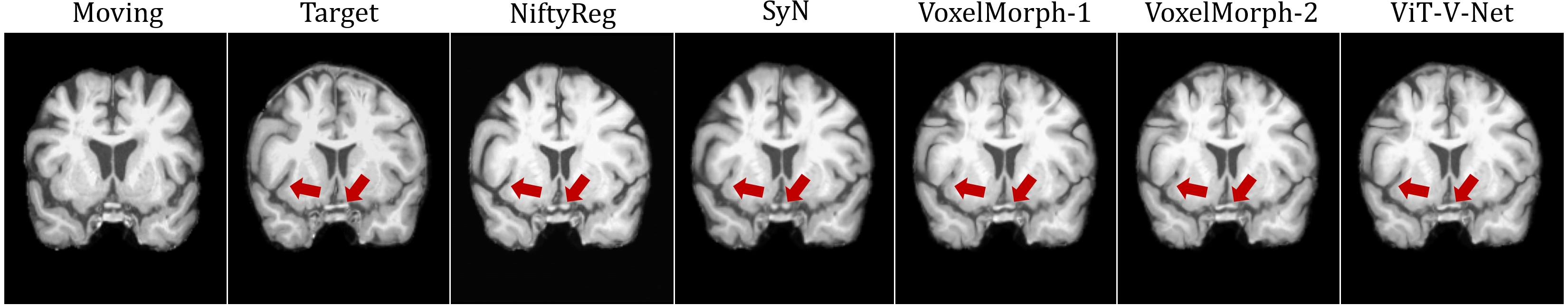
Figure 2: Registration results of a MR coronal slice. Additional results are shown in Appendix D.

3 Results and Conclusions

We demonstrate our method on the task of brain MRI registration. We used an in-house dataset that consists of 260 T1–weighted brain MRI scans. The dataset was split into 182, 26, and 52 (7:1:2) volumes for training, validation, and test sets. Each image volume was randomly matched to two other volumes to form four pairs of $f$ and $m$, resulting in 768, 104, and 208 image pairs. Standard pre-processing steps for structural brain MRI, including skull stripping, resampling, and affine transformation were performed using FreeSurfer [Fischl(2012)]. Then, the resulting volumes were cropped to an equal size of $160\times 192\times 224$. Label maps including 29 anatomical structures were obtained using FreeSurfer for evaluation. The proposed method was compared in terms of Dice score [Dice(1945)] to Symmetric Normalization (SyN) [Avants et al.(2008)Avants, Epstein, Grossman, and Gee], NiftyReg [Modat et al.(2010)], and a learning-based method, VoxelMorph-1 and -2 [Balakrishnan et al.(2018)Balakrishnan, Zhao, Sabuncu, Guttag, and Dalca]. The regularization parameter, $\lambda$, was set to be 0.02, which was reported in [Balakrishnan et al.(2018)Balakrishnan, Zhao, Sabuncu, Guttag, and Dalca] as an optimal value for VoxelMorph. The method was implemented using PyTorch [Paszke et al.(2019)]. Detailed hyperparameter settings for training are shown in Appendix C. Qualitative results, and Dice scores are shown in Table 1 and Fig. LABEL:fig_quali. As visible from the results, the proposed ViT-V-Net yielded a significant gain of $>0.1$ in Dice performance ($p$-values are shown in Table. 4) compared to the others. We also noticed that ViT-V-Net reached lower loss values and had higher validation Dice scores during training (see Fig. LABEL:fig_curve in Appendix D). In conclusion, the proposed ViT-based architecture achieved superior performance than the top-performing registration methods, demonstrating the effectiveness of ViT-V-Net.

This work was supported by a grant from the National Cancer Institute, U01-CA140204. The views expressed in written conference materials or publications and by speakers and moderators do not necessarily reflect the official policies of the NIH; nor does mention by trade names, commercial practices, or organizations imply endorsement by the U.S. Government.

Appendix A Overview of Vision Transformer

A detailed description of ViT can be found in [Dosovitskiy et al.(2020), Vaswani et al.(2017), Chen et al.(2021)].

fig_vit

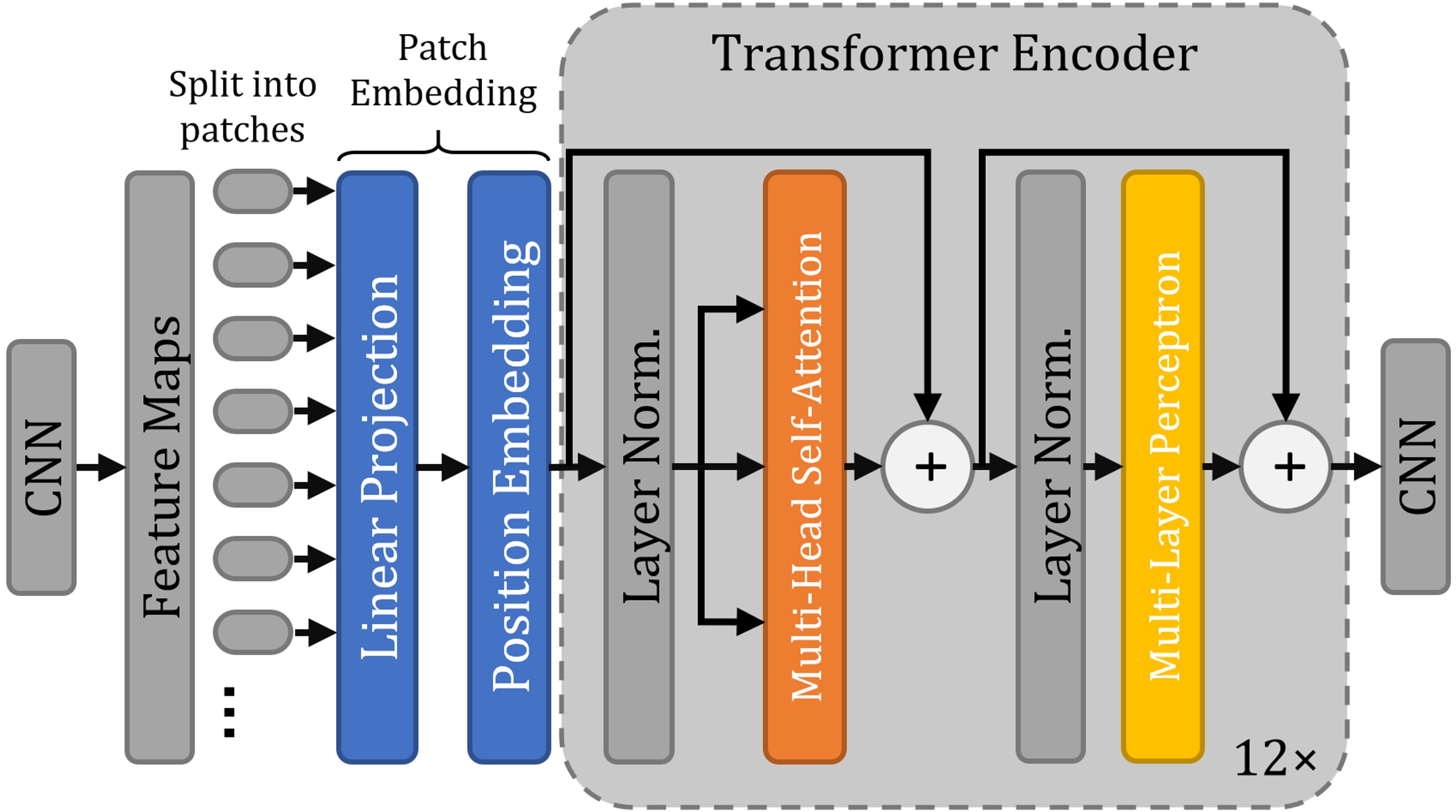
Figure 3: Model overview of the Vision Transformer.

Patch Embedding Let $x_{p}^{i}$ be the $i^{th}$ vectorized patch, where $i\in\{1,...,N\}$. The patches were first encoded into a latent $D$-dimensional space using a trainable linear projection (realized via a convolutional layer). Then, learnable position embeddings were added to retain positional information:

$$\mathbf{z}_{0}=[x_{p}^{1}\mathbf{E};x_{p}^{2}\mathbf{E};...;x_{p}^{N}\mathbf{E}]+\mathbf{E}_{pos},$$ (1)

where $\mathbf{E}\in\mathbb{R}^{P^{3}C\times D}$ denotes the patch embedding projection and $\mathbf{E}_{pos}\in\mathbb{R}^{N\times D}$ represents the positional embedding matrix. Next, the output $\mathbf{z}_{0}$ was fed into consecutive blocks of the Transformer encoder.

Transformer encoder The Transformer encoder consists of 12 blocks of MSA and MLP layers [Vaswani et al.(2017)]. A layer normalization (LN) was applied before each MSA and MLP layer. The output of $\ell^{th}$ Transformer encoder can be written as:

$$\begin{split}\mathbf{z}_{\ell}^{\prime}&=\text{MSA}(\text{LN}(\mathbf{z}_{\ell-1}))+\mathbf{z}_{\ell-1}\\ \mathbf{z}_{\ell}&=\text{MLP}(\text{LN}(\mathbf{z}_{\ell}^{\prime}))+\mathbf{z}_{\ell}^{\prime},\end{split}$$ (2)

where $\mathbf{z}_{\ell}$ denotes the encoded image representation.

Appendix B Loss Functions

The loss function used for training the proposed network can be written as:

$$\mathcal{L}(f,m,\mathbf{\phi})=\mathcal{L}_{MSE}(f,m,\mathbf{\phi})+\lambda\mathcal{L}_{diffusion}(\mathbf{\phi}),$$ (3)

where $\lambda$ is a regularization parameter, $f$ and $m$ are, respectively, the fixed and moving image, and $\mathcal{\phi}$ represents the deformation field.

Image Similarity Measurement The mean squared error (MSE) between the deformed moving image and fixed image was used as the loss function. It is defined as:

$$\mathcal{L}_{MSE}(f,m,\mathbf{\phi})=\frac{1}{\Omega}\sum_{p\in\omega}\left[f(p)-m\circ\mathbf{\phi}(p)\right]^{2},$$ (4)

where $\Omega$ denotes the image domain.

Deformation Field Regularization To enforce smoothness in the deformation field, a diffusion regularizer was used. It is defined as:

$$\mathcal{L}_{diffusion}(\mathbf{\phi})=\sum_{p\in\omega}\|\nabla\mathbf{u}(p)\|^{2},$$ (5)

where $\mathbf{u}$ the displacement field, which is the output of the network.

Appendix C Hyperparameters Settings

	VoxelMoprh-1	VoxelMoprh-2	ViT-V-Net
Optimizer	ADAM	ADAM	ADAM
Learning rate	$1e^{-4}$	$1e^{-4}$	$1e^{-4}$
Learning rate decay	Polynomial (0.9)	Polynomial (0.9)	Polynomial (0.9)
Dropout	$0.0$	$0.0$	$\mathbf{0.1}$
Epochs	$500$	$500$	$500$
Batch size	$2$	$2$	$2$
Loss function	MSE	MSE	MSE
Regularizer	Diffusion	Diffusion	Diffusion
Regularization parameter ($\lambda$)	$0.02$	$0.02$	$0.02$
Data augmentation	Random flipping	Random flipping	Random flipping
ViT patch size ($P$)	-	-	8
ViT latent vector size ($D$)	-	-	252
GPU memory used during training	17.320 GiB	19.579 GiB	18.511 GiB

Table 2: Training setups for the learning-based models. All models were trained using the same optimizer (ADAM [Kingma and Ba(2014)]) and training hyperparameters, except the dropout rate was set to be 0.1 in linear layers of ViT-V-Net. The models were trained and tested on a PC with an AMD Ryzen 9 3900X CPU, an NVIDIA Titan RTX GPU, and an NVIDIA RTX 3090 GPU, where both GPUs have 24 GiB memory. Each model took about 3 days to train on a single GPU.

	Cost fuction	Regularizer	Regularization parameter	Number of iteration
NiftyReg	SSD	Bending energy (default)	0.0002	300, 300, 300 (default)
SyN	MSQ	Gaussian (default)	3 (default)	40, 20, 0 (default)

Table 3: Hyperparameter settings for NiftyReg and SyN, where SSD stands for the sum of squared difference and MSQ stands for the mean squared difference. We chose the regularization parameter for NiftyReg to be 0.0002, because the default value, 0.005, led to over-smoothed suboptimal deformations.

Appendix D Additional Results

	NiftyReg	SyN	VoxelMorph-1	VoxelMorph-2	ViT-V-Net
Dice	0.713$\pm$0.134	0.688$\pm$0.140	0.707$\pm$0.137	0.711$\pm$0.135	0.726$\pm$0.130
% of $|J_{\phi}|\leq 0$	0.225$\pm$0.165	0.118$\pm$0.084	0.375$\pm$0.098	0.414$\pm$0.084	0.381$\pm$0.102
Time (Sec)	113	15.257	0.002	0.002	0.002

Table 4: Quantitative comparisons of Dice score, percentage of voxels with a non-positive Jacobian determinant (i.e., folded voxels), and computational time for different methods. Note that NiftyReg and SyN were applied using the CPUs, while the learning-based methods, VoxelMorph and ViT-V-Net, were implemented on GPU.

	Affine	NiftyReg	SyN	VoxelMorph-1	VoxelMorph-2
ViT-V-Net	$\ll 1e^{-5}$	$4.102e^{-3}$	$\ll 1e^{-5}$	$1.536e^{-5}$	$1.601e^{-3}$

Table 5: $p$-values computed using the paired t-test on the Dice scores between the proposed ViT-V-Net and other registration methods.

fig_curve

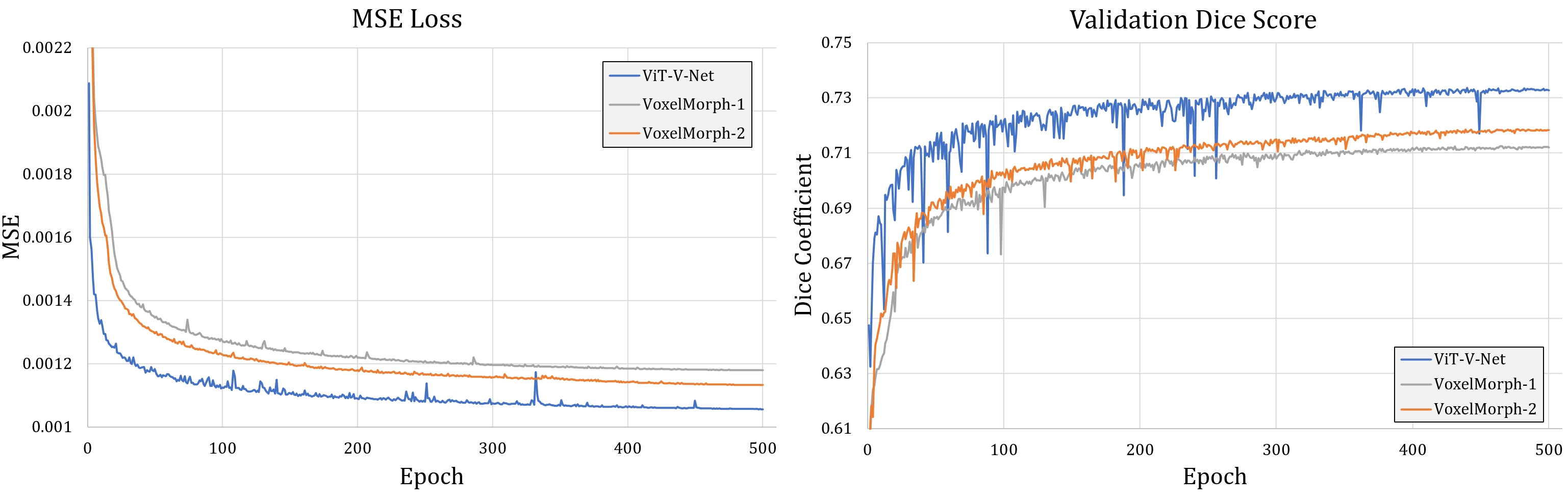
Figure 4: Training loss value and validation Dice score per epoch. The proposed ViT-V-Net exhibits lower loss values and higher Dice scores during training.

fig_vit_res

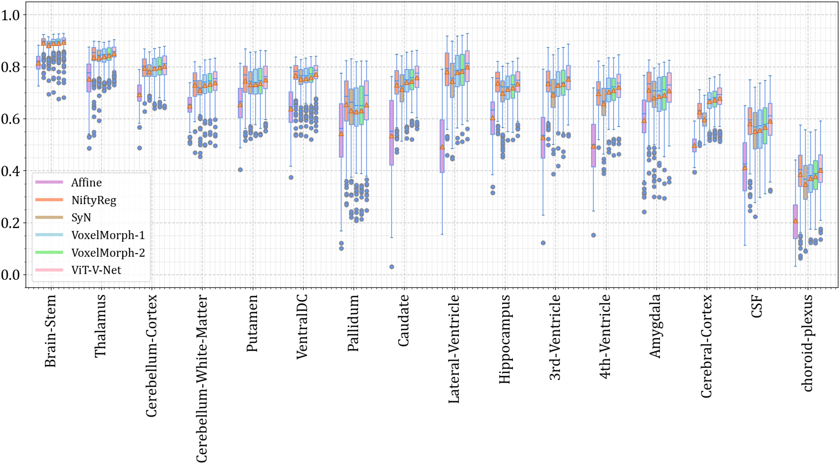
Figure 5: Boxplots of Dice scores for various anatomical structures obtained using different registration methods. Dice scores of the left and right brain hemispheres were averaged into a single score. Orange triangles denote the means.

fig_vit_res

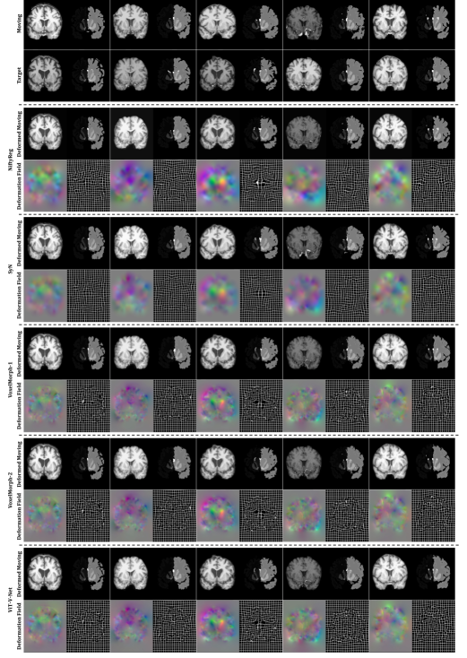
Figure 6: Additional qualitative results generated by different registration methods. The rows in the top panel (of two rows separated by a dashed line) show, respectively, moving and fixed images. The other five panels exhibit deformed images and their corresponding displacement fields produced by different methods. The colored images were created by first clamping the displacement values to a range of $[-10,10]$ and then mapping each spatial dimension to each of the RGB color channels.

References

- [Avants et al.(2008)Avants, Epstein, Grossman, and Gee] Brian B Avants, Charles L Epstein, Murray Grossman, and James C Gee. Symmetric diffeomorphic image registration with cross-correlation: evaluating automated labeling of elderly and neurodegenerative brain. Medical image analysis, 12(1):26–41, 2008.
- [Balakrishnan et al.(2018)Balakrishnan, Zhao, Sabuncu, Guttag, and Dalca] Guha Balakrishnan, Amy Zhao, Mert R Sabuncu, John Guttag, and Adrian V Dalca. An unsupervised learning model for deformable medical image registration. In Proceedings of the IEEE conference on computer vision and pattern recognition, pages 9252–9260, 2018.
- [Beg et al.(2005)Beg, Miller, Trouvé, and Younes] M Faisal Beg, Michael I Miller, Alain Trouvé, and Laurent Younes. Computing large deformation metric mappings via geodesic flows of diffeomorphisms. International journal of computer vision, 61(2):139–157, 2005.
- [Carion et al.(2020)] Nicolas Carion et al. End-to-end object detection with transformers. In European Conference on Computer Vision, pages 213–229. Springer, 2020.
- [Chen et al.(2021)] Jieneng Chen et al. Transunet: Transformers make strong encoders for medical image segmentation. arXiv preprint arXiv:2102.04306, 2021.
- [Chen et al.(2020)Chen, Li, Du, and Frey] Junyu Chen, Ye Li, Yong Du, and Eric C Frey. Generating anthropomorphic phantoms using fully unsupervised deformable image registration with convolutional neural networks. Medical physics, 2020.
- [de Vos et al.(2017)] Bob D de Vos et al. End-to-end unsupervised deformable image registration with a convolutional neural network. In Deep learning in medical image analysis and multimodal learning for clinical decision support, pages 204–212. Springer, 2017.
- [Dice(1945)] Lee R Dice. Measures of the amount of ecologic association between species. Ecology, 26(3):297–302, 1945.
- [Dosovitskiy et al.(2020)] Alexey Dosovitskiy et al. An image is worth 16x16 words: Transformers for image recognition at scale. arXiv preprint arXiv:2010.11929, 2020.
- [Fischl(2012)] Bruce Fischl. Freesurfer. Neuroimage, 62(2):774–781, 2012.
- [Jaderberg et al.(2015)Jaderberg, Simonyan, Zisserman, and Kavukcuoglu] Max Jaderberg, Karen Simonyan, Andrew Zisserman, and Koray Kavukcuoglu. Spatial transformer networks. arXiv preprint arXiv:1506.02025, 2015.
- [Kingma and Ba(2014)] Diederik P Kingma and Jimmy Ba. Adam: A method for stochastic optimization. arXiv preprint arXiv:1412.6980, 2014.
- [Milletari et al.(2016)Milletari, Navab, and Ahmadi] Fausto Milletari, Nassir Navab, and Seyed-Ahmad Ahmadi. V-net: Fully convolutional neural networks for volumetric medical image segmentation. In 2016 fourth international conference on 3D vision (3DV), pages 565–571. IEEE, 2016.
- [Modat et al.(2010)] Marc Modat et al. Fast free-form deformation using graphics processing units. Computer methods and programs in biomedicine, 98(3):278–284, 2010.
- [Paszke et al.(2019)] Adam Paszke et al. Pytorch: An imperative style, high-performance deep learning library. In H. Wallach, H. Larochelle, A. Beygelzimer, F. d'Alché-Buc, E. Fox, and R. Garnett, editors, Advances in Neural Information Processing Systems 32, pages 8024–8035. Curran Associates, Inc., 2019. URL \urlhttp://papers.neurips.cc/paper/9015-pytorch-an-imperative-style-high-performance-deep-learning-library.pdf.
- [Ronneberger et al.(2015)Ronneberger, Fischer, and Brox] Olaf Ronneberger, Philipp Fischer, and Thomas Brox. U-net: Convolutional networks for biomedical image segmentation. In International Conference on Medical image computing and computer-assisted intervention, pages 234–241. Springer, 2015.
- [Sokooti et al.(2017)] Hessam Sokooti et al. Nonrigid image registration using multi-scale 3d convolutional neural networks. In International Conference on Medical Image Computing and Computer-Assisted Intervention, pages 232–239. Springer, 2017.
- [Vaswani et al.(2017)] Ashish Vaswani et al. Attention is all you need. arXiv preprint arXiv:1706.03762, 2017.
- [Vercauteren et al.(2009)Vercauteren, Pennec, Perchant, and Ayache] Tom Vercauteren, Xavier Pennec, Aymeric Perchant, and Nicholas Ayache. Diffeomorphic demons: Efficient non-parametric image registration. NeuroImage, 45(1):S61–S72, 2009.
- [Wang et al.(2020)] Huiyu Wang et al. Axial-deeplab: Stand-alone axial-attention for panoptic segmentation. In European Conference on Computer Vision, pages 108–126. Springer, 2020.
- [Wang et al.(2018)Wang, Girshick, Gupta, and He] Xiaolong Wang, Ross Girshick, Abhinav Gupta, and Kaiming He. Non-local neural networks. In Proceedings of the IEEE conference on computer vision and pattern recognition, pages 7794–7803, 2018.
- [Yu and Koltun(2015)] Fisher Yu and Vladlen Koltun. Multi-scale context aggregation by dilated convolutions. arXiv preprint arXiv:1511.07122, 2015.