A Co-Operative Game Theoretic Approach for the Budgeted Influence Maximization Problem

Abstract

Given a social network of users with selection cost, the Budgeted Influence Maximization Problem (BIM Problem in short) asks for selecting a subset of the nodes (known as seed nodes) within an allocated budget for initial activation to maximize the influence in the network. In this paper, we study this problem under the co-operative game theoretic framework. We model this problem as a co-operative game where the users of the network are the players and for a group of users, the expected influence by them under the Maximum Influence Arborences diffusion model is its utility. We call this game as BIM Game and show this is ‘non-convex’ and ‘sub-additive’. Based on the proposed game-theoretic model and using the solution concept called ‘Shapley Value’, we propose an iterative algorithm for finding seed nodes. The proposed methodology is divided into mainly two broad steps: the first one is computing the approximate marginal gain in Shapley Value for all the nodes of the network, and the second one is selecting seed nodes from the sorted list until the budget is exhausted. We also show that the proposed methodology can even be more effective when the community structure of the network is exploited. The proposed methodologies have been implemented, and an extensive set of experiments have been conducted with three publicly available social network datasets. From the experiments, we observe that the seed set selected by the proposed methodologies lead to more number of influence nodes compared to many standard and baseline methods from the literature with a reasonable computational overhead. In particular, if the community structure of the network is exploited then there is an increase upto $2\%$ in number of influenced nodes.

1 Introduction

The Influence Maximization Problem aims at identifying a small set of highly influential users such that their initial activation leads to the maximum number of influential nodes in the network  Kempe et al. [2003]. This is perhaps one of the most well studied problem in computational social network analysis due to its practical applications in different domains including crowed-sourcing  Hossain [2012], viral marketing  Domingos [2005], computational advertisement  Aslay et al. [2015], recommender systems  Ye et al. [2012] etc. This problem was initially studied by  Kempe et al. [2003] and since then there was an extensive effort to study in and around of this problem. Look into Banerjee et al. [2020], Li et al. [2018] for recent surveys on this topic. The main cause of influence is the diffusion of information and it is basically a cascading effect by which information propagates from one part of the network to the other. To study this process, several diffusion models have been introduced, such as Independent Cascade Model (IC Model), Linear Threshold Model (LT Model), Maximum Influence Arborences Model (MIA Model) and many more Li et al. [2017].

In reality, social networks are formed by rational human agents. This means that if an user is selected as a seed then incentivization is required. However, the basic influence maximization problem assumes that the every users of the network has equal selection cost. though it may not be so in reality. To bridge this gap, Nguyen and Zheng [2013] introduced the ‘Budgeted Influence Maximization Problem’, where the users of the social network are associated with a nonuniform selection cost and a fixed budget is allocated, the goal here is to select a subset of nodes within the allocated budget such that their initial activation leads to maximum number of influenced nodes. As compared to the basic influence maximization problem, existing literature of this problem is very very limited. In this paper, we study this problem under the co-operative game theoretic framework.

Game Theory, which is basically a mathematical study of strategic interaction among a group of rational agents, has been used to solve many problems in the domain of social network analysis such as community detection Chen et al. [2010a], opinion dynamics  Ding et al. [2010], leader selection  Zimmermann and Eguíluz [2005], rumor dissemination  Kostka et al. [2008], influence maximization  Clark and Poovendran [2011] and many more. However, to the best of our knowledge, the BIM Problem has not been studied yet under the game theoretic framework. In this paper, we study the BIM Problem under co-operative game theoretic framework and our study is motivated by the work Narayanam and Narahari [2010]. However, there are the following fundamental differences:

• Narayanam and Narahari [2010]’s study is concentrated on the basic influence maximization problem and the non-uniform nature of the selection cost has not been taken into account, which is a practical concern.

• In their study they have used IC and LT as the underlying diffusion model. However, recently there are several studies on influence maximization that considers MIA Model as the underlying model of diffusion Ke et al. [2018]. In this study also, we have used the MIA as the underlying diffusion model.

• It is well known that the complexity of computing the shapley value of a $n$ player co-operative game is of $\mathcal{O}(n!)$  Narahari [2014]. Even in case of a small size social network (e.g., number of nodes are $100$) this is a huge computational burden. To get rid of this, they have randomly chosen linear number of permutations of the players for computing shapley value Narayanam and Narahari [2010]. However, with the help of an existing result by  Maleki et al. [2013], we use the appropriate number of samples such that shapley value can be computed with bounded error with high probability.

In particular, we make the following contributions in this paper:

• We formulate a co-operative diffusion game for the Budgeted Influence Maximization Problem, and design an iterative algorithm based on the solution concept of a co-operative game known as Shapley value for identifying the influential nodes.

• We study the important properties of the formulated game and detailed complexity analysis of the proposed methodologies have also been done.

• We also show that if we consider the community structure of the network, then the proposed methodology can leads to even more number of influenced nodes.

• The proposed methodologies have been with four publicly available social network datasets and an extensive set of experiments have been carried out to demonstrate the effectiveness of the proposed methodology.

Rest of the paper is organized as follows: Section 2 describes relevant studies from the literature. Section 3 describes required preliminary concepts and define the diffusion game formally. The proposed solution methodologies have been described in Section 4. Section 5 contains the experimental evaluation, and finally, Section 6 concludes our study and gives future directions.

2 Related Work

Our study is closely related to the ‘Influence Maximization in Social Networks’, more particularly the Budgeted Influence Maximization Problem, and also game theoretic solution methodologies for the influence maximization problem. Here, we present relevant studies from the literature.

Influence Maximization in Social Networks

The problem of influence maximization aims at choosing a small number of highly influential users in a social network for initial activation such that due to the cascading effect of diffusion, the number of influenced node is maximized  Kempe et al. [2003].  Domingos and Richardson [2001], Richardson and Domingos [2002] first introduced this problem for the ‘viral marketing’ in social networks. Later on,  Kempe et al. [2003, 2005, 2015] studied the computational issues of this problem and showed that the problem is $\mathcal{NP}$-Hard under the Independent Cascade and Linear Threshold Model of diffusion. However, they gave a $(1-\frac{1}{e})$- factor approximation algorithm, which works based on maximum marginal influence gain computation and $\mathcal{O}(n^{1-\epsilon})$ for any $\epsilon>0$ factor inapproximability result. Their study remains an influential one and triggers a huge amount of study in last one and half decades. Solution methodologies can be grouped into different categories, such as ‘approximation algorithms’ such as CELF  Leskovec et al. [2007b], CELF++  Goyal et al. [2011a], MIA  Wang et al. [2012], PMIA  Wang et al. [2012], TIM  Tang et al. [2014], IMM  Tang et al. [2015]; heuristic solutions such as SIMPATH  Goyal et al. [2011b], IRIE  Jung et al. [2012], LDGA  Chen et al. [2010b], Community-Based Solution Methodologies such as CIM  Chen et al. [2012, 2014], ComPath Rahimkhani et al. [2015], INCIM Bozorgi et al. [2016], CoFIM Shang et al. [2017] and many more. Please refer to Banerjee et al. [2020], HAFIENE et al. [2020], Li et al. [2018] (and references therein) for recent surveys.

Budgeted Influence Maximization Problem

In case of BIM Problem, along with the input social network, we are also given with a cost function that assigns selection cost to each node and a fixed budget is allocated for the seed set selection. Nguyen and Zheng [2013] first introduced the BIM Problem and proposed a $(1-\frac{1}{\sqrt{e}})$-factor approximation algorithm and two efficient heuristics to solve this problem. Recently, Wang and Yu [2020] studied the BIM Problem and proposed a solution methodology that gives an approximation ratio of $\frac{1}{2}(1-\frac{1}{e})$. They further showed that this can be improved upto $(1-\beta)(1-\frac{1}{e})$. Güney [2019] proposed an integer programming-based approach to solve this problem under the IC Model of diffusion. Han et al. [2014] proposed a couple of heuristics for this problem that carefully considers both cost effective nodes and influential nodes. Recently, Banerjee et al. [2019] proposed a community-based solution methodology for the BIM Problem which is broadly divided into four steps, namely, community detection, budget distribution, seed node selection, and budget transfer. Shi et al. [2019] proposed two different solution methodologies with data dependent approximation ratio. Yu et al. [2018] studied this problem under credit distribution model and came up with a streaming algorithm with $(\frac{1}{3}-\epsilon)$ approximation of the optimum.

Game Theoretic Solution Methodologies for SIM and Related Problems

Game theoretic techniques have been used to solve the influence maximization problems since last one decade. To the best of our knowledge, the first study in this direction was by Narayanam and Narahari [2010]. They proposed a ‘Shapley Value’-based approach for selecting the seed nodes for the influential maximization problem. Clark and Poovendran [2011] studied the influence maximization problem in competitive situation and they formulated a Stackleberg Game and proposed a methodology to solve the game. Borodin et al. [2010] studied the influence maximization problem in competitive situation with several natural extensions of the LT Model. Angell and Schoenebeck [2017] studied the influence maximization problem and proposed a greedy heuristic that shows an improvement of $7\%$ and $55\%$ for submodular and non-submodular influence functions, respectively. Li et al. [2015] study the influence maximization problem in competitive situation and proposed a game theoretic framework for this problem. They designed a non-cooperative game and proposed an algorithm that computes the ‘Nash Equilibrium’ of the game that guarantees optimal strategies. Recently, Wang et al. [2020] proposed an cumulative oversampling technique for ‘Thompson Sampling’ to construct optimistic parameter estimates with fewer samples. They showed that their learning algorithms can be used to solve the BIM Problem using less number of samples.

To the best of our knowledge, there does not exist any literature that studies BIM Problem under game theoretic setting. In this paper, we study this Problem under Co-Operative Game Theoretic Framework. In particular, we propose an iterative approach based on the Shapley Value for selecting the influential nodes for the BIM Problem. We also show that the exploitation of community structure helps the proposed methodology to achieve even better influence spread.

3 Preliminary Concepts, Background, and Problem Definition

Here, we present some preliminary definitions. Initially, we start with the social network specific ones.

3.1 Social Network Specific

Definition 1 (Social Network).

A social network is an interconnected structure among a group of human agents formed for social interactions, which is often represented as a graph $G(V,E,P)$. Here, the vertex set $V(G)=\{u_{1},u_{2},\dots,u_{n}\}$ are the set of $n$ users, the edge set $E(G)=\{e_{1},e_{2},\dots,e_{m}\}$ are the $m$ social ties among the users, and $P:E(G)\rightarrow(0,1]$ is the edge weight function that assigns each edge to its influence probability.

We denote the number of nodes and edges of the network by $n$ and $m$, respectively. For any positive integer $n$, $[n]$ denotes the set $\{1,2,\cdots,n\}$. For any $e\equiv(uv)\in E(G)$, we denote the influence probability assigned to it as $P(e)$ or $P_{uv}$. If, $(uv)\notin E(G)$ then $P_{uv}=0$. Now, to start a diffusion process in the network, there should be some initial adopters, which we call as seed nodes. To study the diffusion process in a network, several models have been introduced such as IC Model, LT Model, MIA Model and so on Guille et al. [2013]. Now, once a diffusion process is initiated from a number of seed nodes, it ends with influencing a subset of the nodes and called as the influence of the seed set, which is defined next.

Definition 2 (Influence of a Seed Set).

Given a social network $G(V,E,P)$ and a diffusion model $\mathcal{M}$ for a given seed set $S\subseteq V(G)$, its influence is defined as the number of nodes that are influenced due to the initial activation of the nodes in $S$ if the information is diffused by the rule of the model $\mathcal{M}$. $I_{\mathcal{M}}(S)$ denotes the the set of influenced nodes by the seed set $S$ under the diffusion model $\mathcal{M}$. This quantity is measured in terms of expactation. Hence, the influence of the seed set $S$ and under the diffusion model $\mathcal{M}$ is $\sigma_{\mathcal{M}}(S)=\mathbb{E}(|I_{\mathcal{M}}(S)|)$, where $\sigma(.)$ is the social influence function, i.e., $\sigma:2^{V(G)}\rightarrow\mathbb{R}_{0}^{+}$ with $\sigma(\emptyset)=0$. Here, $\emptyset$ denotes the empty set.

Now, any real-world diffusion processes (such as political campaigns, viral marketing of products etc.) are always carried out to maximize the influence. In this direction, next we state the well studied Social Influence Maximization Problem.

Definition 3 (Social Influence Maximization Problem (SIM Problem)).

Kempe et al. [2003] Given a social network $G(V,E,P)$, a diffusion model $\mathcal{M}$, and a positive integer ($k\in\mathbb{Z}^{+}$), the social influence maximization problem asks for selecting a seed set $S\subseteq V(G)$ with $|S|\leq k$, whose initial activation leads to the maximum number of influenced nodes, if the diffusion process happens by the rule of the model $\mathcal{M}$. Mathematically,

$$S^{*}=\underset{S\subseteq V(G),|S|\leq k}{argmax}\ \sigma_{\mathcal{M}}(S)$$ (1)

As mentioned previously, real-world social networks are formed by rational and self interested agents. If a node is selected as seed then some kind of incentivization is required. In reality, different users of the network have different selection cost, i.e., users have non uniform selection cost. However, the SIM Problem assumes that the selection costs are uniform. To bridge this gap, the ‘Budgeted Influence Maximization Problem’ has been introduced by Nguyen and Zheng [2013] which is defined next.

Definition 4 (Budgeted Influence Maximization Problem).

Given a social network $G(V,E,P)$ along with a cost function $C:V(G)\rightarrow\mathbb{Z}^{+}$ that assigns each node to its selection cost, a diffusion model $\mathcal{M}$, and a fixed budget $B$, the problem of budgeted influence maximization asks for selecting a seed set within the allocated budget, whose initial activation leads to the maximum number of influenced nodes, if the diffusion process happens by the rule of the model $\mathcal{M}$. Mathematically,

$$S^{*}=\underset{S\subseteq V(G),C(S)\leq B}{argmax}\ \sigma_{\mathcal{M}}(S),$$ (2)

where, $C(S)$ denotes the total selection cost of the users in $\mathcal{S}$, i.e., $C(S)=\underset{u\in S}{\sum}C(u)$. We denote an arbitrary instance of BIM Problem as $<G(V,E,P),C,B>$.

From the algorithmic point of view the problem can be posed as follows:

Next, we state the Maximum Influence Aroborance (MIA) diffusion model, which we have considered as the underlying diffusion model. Symbols and notations used in this paper is given in Table 1.

Table 1: Symbols and notations used in this study

Symbol	Meaning
$G(V,E,P)$	The input social network
$V(G)$, $E(G)$	Vertex and Edge set of $G$
$n,m$	The number vertices and edges of $G$
$P$	The edge probability function
$K$	The set of communities of $G$
$\ell$	The number of communities of $G$
$P(e)/P_{uv}$	The edge probability of the edge $e\equiv(uv)$
$\mathcal{P}(p)$	Propagation probability of the path $p$
$C$	The cost function
$C(u)$	Cost of the user $u$
$B$	Budget for seed set selection
$\sigma(.)$	The social influence function
$S$	The seed set
$C(S)$	Total selection cost of the users in $S$
$\sigma(S)$	The influence of the seed set $S$
$p_{u_{i}u_{j}}^{max}$	Maximum influence path from $u_{i}$ to $u_{j}$
$\mathbb{P}(u_{i},u_{j})$	Set of all paths between $u_{i}$ and $u_{j}$
$\theta$	Cut Off Probability
$d_{max}$	Maximum degree of $G$
$N$	The set of players $\{1,2,\ldots,n\}$
$\nu$	The utility/ pay-off function
$(N,\nu)$	The BIM Game
$\Psi_{i}(\mathcal{N},\nu)$	Shapley value of the $i$-th player
$MIIA(v,\theta)$	The set of MIA Paths to the node $v$
$\mathbb{Z}^{+}$	The set of positive integers
$\mathbb{R}_{0}^{+}$	The set of positive real numbers including zero

3.2 The MIA Diffusion Model

This is the diffusion model introduced by Wang et al. [2012]. Before stating the diffusion model first we state two preliminary definitions.

Definition 5 (Propagation Probability of a Path).

Given two vertices $u_{i},u_{j}\in V(G)$, let $\mathbb{P}(u_{i},u_{j})$ denotes the set of paths from the vertex $u_{i}$ to $u_{j}$. For any arbitrary path $p\in\mathbb{P}(u_{i},u_{j})$ the propagation probability is defined as the product of the influence probabilities of the edges that constitute the path.

$$\mathcal{P}(p)=\begin{cases}\underset{(u_{i}u_{j})\in p}{\prod}P_{u_{i}u_{j}}&\text{if $\mathbb{P}(u_{i},u_{j})\neq\phi$}\\ 0&\text{otherwise}\\ \end{cases}$$ (3)

Definition 6 (Maximum Probabilistic Path).

Given two vertices $u_{i},u_{j}\in V(\mathcal{G})$, the maximum probabilistic path is the path with the maximum propagation probability and denoted as $p_{u_{i},u_{j}}^{max}$. Hence,

$$p_{u_{i},u_{j}}^{max}=\underset{p\in\mathbb{P}(u_{i},u_{j})}{argmax}\ \mathcal{P}(p)$$ (4)

Based on the path propagation probability and and maximum probabilistic path maximum influence in-arborescences are defined as follows.

Definition 7 (Maximum Influence In-Arborescences (MIIA)).

For a node $v\in V(G)$, and a probability threshold $\theta$, the maximum influence in-arborescence is the union of the maximum influence paths with more than the cut off probability $\theta$ to $v$. Mathematically,

$$MIIA(v,\theta)=\underset{u\in V(G)\setminus v;p_{u,v}^{max}\geq\theta}{\bigcup}p_{u,v}^{max}$$ (5)

Now, given a seed set $S$, a node $v\in V(G)\setminus S$ and its $MIIA(v,\theta)$, by the rule of $MIA$ model it is assumed that the influence from $S$ to $v$ is propagated through the paths in $MIIA(v,\theta)$. Let $ap(u,S,MIIA(v,\theta))$ be the influence probability of the node $u$ by the seed set $S$ and this can be recursively computed as mentioned in Wang et al. [2012].

Definition 8 (MIA Diffusion Model).

For any seed set $S\subseteq V(G)$ and any arbitrary node $v\in V(G)\setminus S$, in the MIA Model, it is assumed that the nodes in $S$ will influence $v$ through the paths in $MIIA(v,\theta)$ and the expected influence by the seed set $S$ can be given by the Equation 6

$$\sigma(S)=\underset{v\in V(G)}{\sum}ap(v,S,MIIA(v,\theta))$$ (6)

The following two lemmas will be useful to prove some properties of the diffusion game, which will be defined later.

Lemma 1.

Wang et al. [2012] The influence function mentioned in Equation 6 is non-negative, and monotone (i.e., $\forall S\subseteq V(G)$, $\sigma(S)\geq 0$ and $\forall S\subseteq T\subseteq V(G)$, $\sigma(S)\leq\sigma(T)$).

Lemma 2.

Wang et al. [2012] The influence function mentioned in Equation 6 is submodular (i.e., $\forall S\subseteq T\subseteq V(G)$, and $u\in V(G)\setminus T$ and $\sigma(S\cup\{u\})-\sigma(S)\geq\sigma(T\cup\{u\})-\sigma(S)$.

3.3 Co-Operative Game Theory Specific

Co-operative game theory is the study about strategic formation of coalition and their mathematical analysis which is defined next.

Definition 9 (Co-Operative Game or Coalition Game or Transferable Utility Game).

A Co-Operative Game is defined by the tuple $(\mathcal{N},\nu)$, where $\mathcal{N}=\{1,2,\dots,n\}$ is the finite set of players and $\nu$ is called the payoff function (also known as the characteristic function) that assigns each possible coalition to a real number, i.e., $\nu:2^{\mathcal{N}}\rightarrow\mathbb{R}^{+}$. It is assumed that $\nu(\emptyset)=0$.

In co-operative game theory, one of the main concern is how to distribute the total utility among the players. It is called as the payoff allocation.

Definition 10 (Payoff Allocation).

A payoff allocation is a vector $v=(v_{i})_{i\in\mathcal{N}}$ in $\mathbb{R}^{\mathcal{N}}$, where each entry represents the utility share to the corresponding player.

The Shapley Value is an important solution concept in co-operative game theory, which performs the payoff allocation satisfying the following three properties, namely, symmetry, linearity, and carrier Narahari [2014].

Definition 11 (Shapley Value).

In a co-operative game $(\mathcal{N},\nu)$, the Shapley Value of the player $i$ towards a coalition $\mathcal{T}$ is defined as

$$\Psi_{i}(\mathcal{N},\nu)=\underset{\mathcal{T}\subseteq\mathcal{N}\setminus\{i\}}{\sum}\frac{|\mathcal{T}|!*(|\mathcal{N}|-|\mathcal{T}|-1)!}{|\mathcal{N}|!}(\nu(\mathcal{T}\cup\{i\})-\nu(\mathcal{T}))$$ (7)

4 Proposed Methodology

In this section, we describe the game theoretic approach for solving the BIM Problem. This section is broadly divided into the following subsections. In Sub-section 4.1, we define the BIM Game and establish its properties. Sub-section 4.2 contains the overview of the proposed methodology. Sub-section 4.3 contains the algorithms present in the proposed methodology, and finally, Sub-section 4.4 contains time and space complexity analysis of our proposed approaches.

4.1 The BIM Game and Its Properties

Definition 12 (The BIM Game).

We define our diffusion game as a co-operative game, where the nodes of the network are the players, and for any subset of players, their utility is the expected influence in the network under the MIA Model of diffusion. We denote this diffusion game as $(\mathcal{N},\nu)$, where $\mathcal{N}=V(G)=\{u_{1},u_{2},\ldots,u_{n}\}$, $\nu:2^{V(G)}\longrightarrow\mathbb{R}^{+}$, and for any $S\subseteq V(G)$, $\nu(S)=\sigma(S)$ .

Now, we show some of the important properties of the utility function and the proposed diffusion game.

Proposition 1 (Non-negativity and Monotonicity of $\nu(.)$).

The utility function of the diffusion game in Definition 12 is non-negative and monotone.

Proof.

As mentioned in Lemma 1, under MIA diffusion model, the influence function is non-negativity and monotone, the same holds for the utility function as well. ∎

Proposition 2 (Non-Convexity of the Diffusion Game).

The BIM Game defined in Definition 12 is not convex.

Proof.

By definition, a co-operative game is said to be convex, if its utility function $\nu(.)$ has the following property: for all $S\subseteq T\subseteq\mathcal{N}$ and for all $u\in\mathcal{N}\setminus T$, $\nu(S\cup\{u\})-\nu(S)\leq\nu(T\cup\{u\})-\nu(T)$. As mentioned in Lemma 2, the influence function $\sigma(.)$ is submodular, this implies that the diffusion game can not be convex. ∎

Proposition 3 (Sub-Additivity of the BIM Game).

The BIM Game mentioned in Definition 12 is sub-additive.

Proof.

Let, $\mathcal{U}_{1}$ and $\mathcal{U}_{2}$ be two coalition of the BIM Game $(N,\nu)$. Now, we need to show that the utility of the larger coalition, i.e., $\mathcal{U}_{1}\cup\mathcal{U}_{2}$ is at most as the total utility of the individual coalition; i.e.; $\nu(\mathcal{U}_{1}\cup\mathcal{U}_{2})\leq\nu(\mathcal{U}_{1})+\nu(\mathcal{U}_{2})$.

$\nu(\mathcal{U}_{1}\cup\mathcal{U}_{2})=\underset{u\in\mathcal{U}_{1}\cup\mathcal{U}_{2}}{\sum}\nu(u)$

$\Rightarrow\nu(\mathcal{U}_{1}\cup\mathcal{U}_{2})=\underset{u_{i}\in\mathcal{U}_{1}}{\sum}\nu(u_{i})+\underset{u_{j}\in\mathcal{U}_{2}}{\sum}\nu(u_{j})-\underset{u_{x}\in\mathcal{U}_{1}\cap\mathcal{U}_{2}}{\sum}\nu(u_{x})$

$\Rightarrow\nu(\mathcal{U}_{1}\cup\mathcal{U}_{2})=\nu(\mathcal{U}_{1})+\nu(\mathcal{U}_{2})-\underset{u_{x}\in\mathcal{U}_{1}\cap\mathcal{U}_{2}}{\sum}\nu(u_{x})$

$\Rightarrow\nu(\mathcal{U}_{1}\cup\mathcal{U}_{2})\leq\nu(\mathcal{U}_{1})+\nu(\mathcal{U}_{2})$

Hence, it is proved that the BIM Game is sub-additive. ∎

4.2 Overview of the Proposed Methodologies

Here, we describe the shapley value-based iterative approach for identifying the influential users from a social network for the BIM Problem. The proposed methodology is broadly divided into two steps: (i) Shapley Value Computation, and (ii) Seed Set Selection. Now, we explain both these steps in detail.

Step 1 (Shapley Value Computation):

In this step, the Shapley value for all the nodes of the network are computed. As mentioned previously, the Shapley value of a node is basically, the average of the marginal contributions over all possible grand coalition. Now, for forming the grand coalition players may arrive at any order. Certainly, there are $n!$ possible ways to form the grand coalition. Hence, by starling approximation, the growth of $n!$ is basically of $\mathcal{O}(n^{n})$; i.e.; exponential Cormen et al. [2009]. Hence, even for a small size network (let’s say, comprising of $100$ nodes, though real-world networks are much much larger) exact computation of shapley value is not feasible. Hence, to get rid of this problem, we use a result from an existing study by Maleki et al. [2013]. Their study shows that if the range of the marginal contribution of the players are known, it is possible to compute the shapley value of the players with bounded error and high probability. Particularly, if the number of permutations (denoted by $\tau$) considered is greater than or equal to $\left\lceil\frac{ln(\frac{2}{\delta}).r^{2}}{2.\epsilon^{2}}\right\rceil$, then the probability that the incurred error in shapley value computation for any of the players is bounded by $\epsilon$ with probability $1-\delta$. By this principle, for a given $\epsilon$, $\delta$, and $r$ value, we can easily calculate the number of permutations required to consider for shapley value computation such that all the conditions are met. Algorithm 1 describes this procedure.

Step 2 (Seed Set Selection):

Based on the computed shapley value, we select the seed nodes using the following ways:

• Method 1: Once the shapley value of the players are computed, we sort them based on these values and iteratively pick up users as seed nodes until the budget is exhausted. However, in each iteration once a node has been picked up as a seed node, if un-flag its neighbors so that these can not be selected as seed. This will help the proposed methodology to uniformly spread the seed nodes across the network. Algorithm 2 describes this procedure.

• Method 2: In this method, we detect the inherent community structure of the network. For this purpose the Louvian Algorithm Blondel et al. [2008] has been used in our study. After that the total allocated budget has been divided among the communities proportional to the shapley value of the nodes. Based on this shared budget, from each of the communities high shapley value nodes are chosen as seed nodes until the budget is exhausted. If there are any extra budget during seed set from the communities, then it is transferred to the largest community. Algorithm 3 describes this procedure.

Next, we describe both the methodologies in detail in the next subsection.

4.3 Algorithms in the Proposed Methodology

Now, we describe the proposed approaches in the form of algorithms. Algorithm 1 reports the Step 1 of our proposed methodology. The working principle of this algorithm is as follows: Given $\epsilon$, $\delta$, and $r$, first we generate the number of permutations required for shapley value computation. Next, for each permutation we compute the marginal gain of the nodes. In Algorithm 1, $S_{u}(p_{i})$ denotes the set of nodes that appeared before $u$ in the permutation $p_{i}$. First, we activate the first node in the permutation and compute the influence. Next, we consider the second node in the permutation. If it is already activated by the first node then its marginal contribution is $0$. If it is not activated then we compute the marginal gain by subtracting the individual influence from the combined influence. In this way, we compute the marginal gain of all the nodes of the network. We repeat this process for $\mathcal{R}$ (part of input) given number of times. Now, we compute the marginal gain by dividing $\mathcal{R}$. Finally, the shapley value is computed by dividing the number of permutations considered in shapley value computation.

It is important to observe that Algorithm 1 takes the range of marginal gain of the players as one of the input among many. Now, we mention the way we compute this quantity. For any node $u\in V(G)$, we compute its range as follows: Consider the neighbors of the node, i.e., $N(u)$. Consider a node $w\in N(u)$. Now, $w$ can be influenced by any of its neighbors. The upper value of this range is $(\frac{deg(u)}{2}+\underset{w\in N(u)}{\sum}\frac{1}{deg(w)-1})$. In the worst case may be none of the neighbors will be influenced, and hence, the lower value of the range is $0$. So, the range of the marginal gain of the player $u$ is $[0,\frac{deg(u)}{2}+\underset{w\in N(u)}{\sum}\frac{1}{deg(w)-1}]$. After computing the range of all the players, we aggregate them by taking average over all the players; i.e., $r=\frac{\underset{u\in V(G)}{\sum c_{u}}}{n}$.

As mentioned, after computing the shapley value of the players the next step is to choose the seed nodes. Algorithm 2 describes the Method 1. Though Algorithm 2 easy to understand and simple to implement, still we can improve the performance of this algorithm by exploiting the community structure of the network. Algorithm 3 describes that procedure.

Data: A BIM Problem Instance $<G(V,E,P),C,B>$, Error $\epsilon$, Probability $\delta$, and Range of Marginal Contribution $r$.

Result: The array $\phi$ containing the shapley value of the nodes.

1 for $u\in V(G)$ do

2       $b_{u}\longleftarrow 0$;

3       $c_{u}\longleftarrow\frac{deg(u)}{2}+\underset{w\in N(u)}{\sum}\frac{1}{deg(w)-1}$;

4      

5 end for

6$r=\frac{\underset{u\in V(G)}{\sum c_{u}}}{n}$;

7 Generate $\tau\geq\left\lceil\frac{ln(\frac{2}{\delta}).r^{2}}{2.\epsilon^{2}}\right\rceil$ number of permutations of the players;

8 Computation repeats for $\mathcal{R}$ times ;

9 Create the arrays $\phi$ and $MG$, each of size $n$ and initialize them with $0$;

10 for  $i=1\text{ to }\tau$ do

11       for  $u\in V(G)$ do

12             $T(u)=0$;

13            

14       end for

15      for  $j=1\text{ to }\mathcal{R}$ do

16             for  $u\in V(G)$ do

17                   $T(u)=T(u)+\nu(S_{u}(p_{i})\cup\{u\})-\nu(S_{u}(p_{i}))$;

18                  

19             end for

20            $MG(u)=\frac{T(u)}{\mathcal{R}}$;

21            

22       end for

23      

24 end for

25for  $u\in V(G)$ do

26       $\phi(u)=\frac{MG(u)}{\tau}$;

27      

28 end for

Return the array $\phi$ containing the shapley value of the nodes

Algorithm 1 Step 1: Algorithm for Computing Approximate Shapley Value Computation

Data: A BIM Problem Instance $<G(V,E,P),C,B>$, The array $\phi$.

Result: The seed set for diffusion $S$, such that $C(S)\leq B$.

1 $N\longleftarrow$ Sort the players based on the shapley value computed in $\phi$. ;

2 $S=\emptyset$;

3 Declare the array Flag of size $n$ and initialize each entry by $1$ ;

4 for $i=1\text{ to }n$ do

5       while $B>0$ do

6             if $B\geq C(u_{i})\text{ and }Flag(u_{i})==1$ then

7                   $S\longleftarrow S\cup\{u_{i}\}$;

8                   $B\longleftarrow B-C(u_{i})$;

9                  

10             end if

11            for $\text{All }v\in\mathcal{N}(u_{i})$ do

12                   $Flag(v)\longleftarrow 0$;

13                  

14             end for

15            

16       end while

17      

18 end for

Return the set $S$ as seed set.

Algorithm 2 Step 2: Influential Node Selection (Method $1$)

Data: A BIM Problem Instance $<G(V,E,P),C,B>$, The array $\phi$.

Result: The seed set for diffusion $S$, such that $C(S)\leq B$.

1 $Community\longleftarrow\text{Detect the Community Structure of the Network}$;

2 $K\longleftarrow\{K_{1},K_{2},\ldots,K_{\ell}\}$; $K\longleftarrow Sort(K)$;

3 $K_{max}\longleftarrow Largest\_Community(K)$; $Total\_Shapley\longleftarrow 0$;

4 for $\text{All }u\in N$ do

5       $Total\_Shapley=Total\_Shapley+\phi(u)$;

6      

7 end for

8Create the array $B_{K}$ and initialize all entries with $0$;

9 for $i=1\text{ to }\ell$ do

10       $Temp\_Shapley\longleftarrow 0$;

11       for $\text{All }u\in V(K_{i})$ do

12             $Temp\_Shapley=Temp\_Shapley+\phi(u)$;

13            

14       end for

15      $B_{K_{i}}\longleftarrow\frac{Temp\_Shapley}{Total\_Shapley}.B$

16 end for

17$S\longleftarrow\emptyset$;

18 for $i=1\text{ to }\ell$ do

19       $V(K_{i})\longleftarrow$ Sort the nodes in $V(K_{i})$ based on the value computed in $\phi$;

20       for $j=1\text{ to }|V(K_{i})|$ do

21             while $B_{K_{i}}\geq 0$ do

22                   if $B_{K_{i}}\geq C(u_{j})$ then

23                         $S\longleftarrow S\cup\{u_{j}\}$;

24                         $B_{K_{i}}\longleftarrow B_{K_{i}}-C(u_{j})$;

25                        

26                   end if

27                  

28             end while

29            

30       end for

31      $B_{K_{max}}\longleftarrow B_{K_{max}}+B_{K_{i}}$;

32      

33 end for

Return the set $S$ as seed set.

Algorithm 3 Step 2: Influential Node Selection (Method $2$)

4.4 Complexity Analysis of the Proposed Methodologies

Now, we analyze the algorithms to understand the running time and space requirement for the proposed methodologies. From Line $1$ to $5$, we compute the range of marginal gain of the players. This can be implemented in $\mathcal{O}(n^{2})$ time and $\mathcal{O}(n)$ space. Degrees of all the nodes can be computed in $\mathcal{O}(n^{2})$ time. Now, assume that $d_{max}$ denotes the maximum degree of all the nodes; i.e.; $d_{max}=\underset{u\in V(G)}{max}\ deg(u)$. Hence, for a particular player $u\in V(G)$, the instruction mentioned in Line 3 can be computed in $\mathcal{O}(d_{max})$ time. The execution time of Line No $5$ is of $\mathcal{O}(n)$. Hence, the computational time from Line $1$ to $5$ is of $\mathcal{O}(n^{2}+nd_{max}+n)$. As, $d_{max}$ is upper bounded by $\mathcal{O}(n)$, hence the quantity reduces to $\mathcal{O}(n^{2})$. It is important to observe that marginal contribution of any player can be computed by traversing the graph, which takes $\mathcal{O}(m+n)$. In each permutation, there are $n$ players. Hence, considering $\tau$ number of permutations and repeating the same experiment for $\mathcal{R}$ times requirement for marginal gain computation is of $\mathcal{O}(\tau\cdot n\cdot(m+n)\cdot\mathcal{R})$ time. After that, computing the shapley value requires additional $\mathcal{O}(n)$ time. Hence, total time requirement is of $\mathcal{O}(n^{2}+\tau\cdot n\cdot(m+n)\cdot\mathcal{R})$ and this reduces to $\mathcal{O}(\tau\cdot n\cdot(m+n)\cdot\mathcal{R})$. The extra space consumed by the Algorithm 1 is to store the arrays $T$, $MG$, $\phi$, also to store the degree of the nodes and all of them requires $\mathcal{O}(n)$ space each. Hence the Lemma 3 holds.

Lemma 3.

Running time and space requirement of Algorithm 1 is of $\mathcal{O}(\tau\cdot n\cdot(m+n)\cdot\mathcal{R})$ and $\mathcal{O}(n)$, respectively.

As mentioned previously, once the shapley value of the players are computed, the seed set can be selected either of the two ways. In Algorithm 2, first the nodes of the players are sorted based on the shapley value computed in Algorithm 1. This step requires $\mathcal{O}(n\log n)$ time. Let, $d_{max}$ denotes the maximum degree of the network. Now, from Line $4$ to $14$ requires $\mathcal{O}(nd_{max})$ time. Hence, the running time of Algorithm 2 is of $\mathcal{O}(n\log n+nd_{max})$ time. Extra space required by Algorithm 2 is to store the array $Flag$ and the seed set $S$, which is of $\mathcal{O}(n+|S|)=\mathcal{O}(n)$. Hence, Lemma 4 holds.

Lemma 4.

The running time and space requirement of Algorithm 2 is of $\mathcal{O}(n\log n+nd_{max})$, and $\mathcal{O}(n)$, respectively.

Algorithm 3 describes another way of selecting seed nodes. In this method, first the community structure is detected. This can be done by the Louvian Algorithm, which takes $\mathcal{O}(n\log n)$ time . The array $Community$ stores the community number corresponding to each user, i.e., $Community[i]=x$ means the user $u_{i}$ belongs to the $x$-th community of the network. Assume that there are $\ell$ number of communities of the network. Sorting the communities will require $\mathcal{O}(\ell\log\ell)$ time. Computing the total shapley value of the network requires $\mathcal{O}(n)$ time. Line $10$ to $16$ actually shows the budget distribution among the communities, which takes $\mathcal{O}(n\ell)$ time. Line $18$ to $29$ describes the seed set selection process. Now, it is important to observe that the running time of this phase depends upon the number of nodes that the community contains. To give a weak upper bound, we first calculate the running time for the seed selection for the largest community, and then multiply it with the number of communities. Let, $n_{max}$ denotes the number of nodes in the largest community. $\mathcal{O}(n)$ time is required to identify the nodes belongs to that community and sorting them based on the values computed in the array $\phi$ requires $\mathcal{O}(n_{max}\log n_{max})$ time. Now, selecting the nodes from the sorted list requires $\mathcal{O}(n_{max})$ time. So, the time requirement for the execution of the largest is of $\mathcal{O}(n+n_{max}\log n_{max}+n_{max})=\mathcal{O}(n+n_{max}\log n_{max})$. Additionally, during the processing of communities other than the largest one, transferring the unutilized budget of the community to the largest community requires $\mathcal{O}(1)$ time. Hence, time requirement for the execution from Line $18$ to $29$ requires $\mathcal{O}(n\ell+\ell n_{max}\log n_{max}+\ell)=\mathcal{O}(n\ell+\ell n_{max}\log n_{max})$. Hence, total time requirement of Algorithm 3 requires $\mathcal{O}(n\log n+\ell\log\ell+n\ell+n\ell+\ell n_{max}\log n_{max})=\mathcal{O}(n\log n+\ell\log\ell+n\ell+\ell n_{max}\log n_{max})$. Extra space consumed by Algorithm 3 is to store the array $Community$, which requires $\mathcal{O}(n)$ space; the array $B_{K}$, which requires $\mathcal{O}(\ell)$ space, vertices of the communities during seed set selection, which requires $\mathcal{O}(n_{max})$ space, and storing the seed set which requires $\mathcal{O}(|S|)$ space. Hence, total space requirement of Algorithm 3 is of $\mathcal{O}(n+\ell+n_{max}+|S|)=\mathcal{O}(n+\ell)$. Hence, Lemma 5 holds.

Lemma 5.

Running time and space requirement of Algorithm 3 is of $\mathcal{O}(n\log n+\ell\log\ell+n\ell+\ell n_{max}\log n_{max})$ and $\mathcal{O}(n+\ell)$, respectively.

Now, after computing the shapley value by Algorithm 1, if we use Algorithm 2 for selecting the seed nodes then the running time and space requirement of the proposed methodology becomes is of $\mathcal{O}(\tau(m+n)R+n\log n+nd_{max})$, and $\mathcal{O}(n)$, respectively. Otherwise, if we use Algorithm 3 for seed set selection then the running time and space requirement of the proposed methodology becomes $\mathcal{O}(\tau\cdot n\cdot(m+n)\cdot\mathcal{R}+n\log n+\ell\log\ell+n\ell+\ell n_{max}\log n_{max})$, and $\mathcal{O}(n+\ell)$, respectively. Hence, from Lemma 3, 4, and 5, following two theorems are implied.

Theorem 1.

If Algorithm 2 is used for seed set selection then the running time and space requirement of our proposed methodology becomes $\mathcal{O}(\tau\cdot n\cdot(m+n)\cdot\mathcal{R}+n\log n+nd_{max})$, and $\mathcal{O}(n)$, respectively.

Theorem 2.

If Algorithm 3 is used for seed set selection then the running time and space requirement of our proposed methodology becomes $\mathcal{O}(\tau\cdot n\cdot(m+n)\cdot\mathcal{R}+n\log n+\ell\log\ell+n\ell+\ell n_{max}\log n_{max})$, and $\mathcal{O}(n+\ell)$, respectively.

5 Experimental Evaluation

In this section, we describe the experimental evaluation of the proposed methodologies. Also, the obtained results have been compared with that of results obtained from the existing methods from the literature. Initially, we start with a brief description of the datasets used in our experiments.

5.1 Datasets

We use the following three datasets appeared in two different situations. First two datasets are basically collaboration networks among the researchers of two different areas. The third one is the trust network among the users of the E-Commerce house epinions.com.

• HEP Theory Collaboration Network (HEPT) Leskovec et al. [2007a] : This dataset contains the collaboration information among the high energy physics researchers obtained from the papers submitted in the high energy physics section of arxiv.org. Here, individual researchers are the nodes and two nodes are linked by an edge if the corresponding researchers co-authored atleast one paper.

• Condensed Matter Physics Collaboration Network (CMP) Leskovec et al. [2007a]: This is also a collaboration network and obtained by connecting the researchers of the condensed matter physics section of the arxiv.org.

• Epinions Dataset Richardson et al. [2003]: This dataset contains ‘who trust whom’ information among the users of a review site named ‘Epinions’. Here, the users form the vertex set of the network and there is a directed edge between $u_{i}$ and $u_{j}$ if and only if $u_{i}$ trusts $u_{j}$.

All these datasets have been previously used in the experimentation in the domain of influence maximization Jung et al. [2012], Tong et al. [2016], Wen and Deng [2020]. Table 2 contains basic statistics of the mentioned datasets.

Table 2: Basis Statics of the Datasets

Dataset Name	Type	$n$	$m$	$d_{avg}$	$|K|$	Modularity
HEPT	Undirected	9877	25998	5.26	481	0.76382
CMP	Undirected	23133	93497	8.08	20	0.68561
Epinions	Directed	75879	508837	13.41	296	0.79866

5.2 Experimental Setup

Now, we state the experimental set up that has been used in this paper. Following parameters are there in our study whose value need to be set:

• Selection Cost: We assign an integer values as the selection cost of the users from the interval $[50,100]$ uniformly at random. In Nguyen and Zheng [2013]’s study also cost of the users are chosen randomly from a fixed interval.

• Budget: In our experiments, we start with a budget value of $2000$ and each time incremented by $4000$ and continued till $26000$. Hence, we experiment with following budget values $B=\{2k,6k,10k,14k,18k,22k,26k\}$. In Nguyen and Zheng [2013]’s study also experimentation is carried out with some fixed budget values.

• Influence Probability: As per the existing studies in the literature, in this study also we consider the following three influence probability settings:

  • Uniform: In this setting, every edge of the network is associated with the same probability value. In this study, we consider this fixed value as $0.1$ and $0.2$. These two value has been considered by many existing studies.

  • Tri-Valency: In this setting all the edges of the network are assigned with a fixed probability from the set $\{0.1,0.01,0.001\}$ uniformly at random. This setting has also been considered in many existing studies in the literature.

  • Weighted Cascade: In this setting every edge $(uv)$ has the influential probability which is equal to the reciprocal of the degree of $v$; i.e.; $P_{uv}=\frac{1}{deg(v)}$. In case of directed network $deg(v)$ will be replaced by $indeg(v)$. This setting is also common in many existing studies.

  All these influence probability settings have been used in existing studies in and around the influence maximization problem Hong and Liu [2019], Chen et al. [2010b], Logins and Karras [2019], Cohen et al. [2014].

• Range of the marginal gain of each player: As mentioned previously, to compute the shapley value of a node, we need to know its range of the marginal gain of the players. For any node $u\in V(G)$, we compute its range as follows: Consider the neighbors of the node, i.e., $N(u)$. Consider a node $w\in N(u)$. Now, $w$ can be influenced by any of its neighbors. The upper value of this range is $(\frac{deg(u)}{2}+\underset{w\in N(u)}{\sum}\frac{1}{deg(w)-1})$. In the worst case may be none of the neighbors will be influenced, and hence, the lower value of the range is $0$. So, the range of the marginal gain of the player $u$ is $[0,\frac{deg(u)}{2}+\underset{w\in N(u)}{\sum}\frac{1}{deg(w)-1}]$.

5.3 Goals of the Experiment

Here, we mention the goals of the experiments, which are mentioned below:

• The primary goal of our experimentation is to make a comparative study among the proposed as well as existing methodologies regarding the quality of the seed set that they can select.

• Our second concern is the computational time. We also make a comparative study of the proposed as well as baseline methods based on their computational time requirement.

5.4 Algorithms in the Experiment

Now, we mention the algorithms that are there in our experiments:

5.4.1 Algorithms Proposed in this Paper

• BIM with Co-Operative Game Theory (BIMGT): In this method, the marginal contribution in ‘shapley value’ for every user of the network is computed and the users are sorted based o this value. Users are chosen from this sorted list until the budget is exhausted. This is basically ‘Method 1’ of this paper.

• BIM with Co-Operative Game Theory and Community Structure (BIMGTC): In this method, first the community structure of the network has been exploited and based on the total shapley value of the nodes of the community the total budget is divided among the communities. Subsequently, the nodes with high shapley value is chosen as seed nodes from each of the communities until the allocated budget from each of the communities are exhausted.

5.4.2 Algorithms from the Literature

We compare the performance of the proposed solution approaches with the following existing methods from the literature:

• Random (RAND): In this method, starting with an empty seed set in each iteration among the non-seed nodes any arbitrary node is chosen uniformly at random and put it into the seed set. This process is repeated until the allocated budget is exhausted. Many existing studies considers this method as a baseline Kempe et al. [2003], Wu et al. [2014].

• Maximum Degree Heuristic (MDH): In this method the nodes are sorted based on its degree. Next, the high degree nodes are chosen as the seed set until the budget is exhausted. This method has been used in many existing studies on influence maximization Narayanam and Narahari [2010], Wu et al. [2014], Shang et al. [2017].

• Maximum Clustering Co-efficient Heuristic (MCCH): Working principle of this method is same as the MDH, though instead of degree, in this method the clustering co-efficient of the nodes are computed. Nodes are sorted based on this value and the nodes with high clustering efficient values are chosen as seed nodes unless the allocated budget is exhausted. Existing studies on influence maximization have used this method as a baseline Narayanam and Narahari [2010].

• DAG Based Heuristic for BIM Problem (DAGHEU) Nguyen and Zheng [2013]: This is the first study on the BIM Problem that contains a number of solution methodologies. Among them we compare the performance of our proposed methodologies with DAG1-SPBP. This is the most efficient and effective as per their claim.

• Balanced Seed Selection Heuristic (BSSH) Han et al. [2014]: In this method, first the nodes are divided into two groups: one is ‘cost effective’ nodes and ‘influential’ nodes. Finally, the seed nodes are chosen in an intelligent way from both the sets in an efficient way.

• Community-Based Approach for the BIM Problem Banerjee et al. [2019]: This is the first community-based solution approach for the BIM Problem by Banerjee et al. [2019]. In this method the total allocated budget is divided based on ‘node fraction’ and ‘cost fraction’ among the communities. Subsequently, the high degree nodes from the communities are chosen as seed nodes until the community specific budget is exhausted.

All these methodologies have been implemented in Python 3.4 + NetworkX 2.0.1 environment. Experiments of this study are performed in an workstation with Intel® Xeon(R) W-1290 CPU 3.20GHz × 20 and 16 GB of RAM.

5.5 Experimental Results with Discussions

Now, we describe the experimental results with detailed discussion. First we discuss the impact of influence spread for different budget values by different algorithms.

5.5.1 Impact of Influenced Spread

Figure 1 shows the budget vs. number of influenced nodes plots for the HEPT dataset under different influence probability settings. From this figure it can be observed that the seed set selected by the proposed methodologies leads to the more number of influenced nodes compared to the baseline methods. Now, we give one example. For uniform probability setting with $p_{c}=0.2$ and $\mathcal{B}=26000$, among the existing methodologies the seed set selected by BIMGTC leads to the maximum number of influenced nodes which is $3781$. On the other hand, among the existing methods the seed set chosen by ComBIM leads to the maximum number of influenced nodes which is $3362$. This is almost $12.5\%$ more compared to the ComBIM. This observation is consistent over different influence probability settings. From Table 2, it can be observed that the number of nodes of the HEPT dataset is $9877$. Hence, the influence coverage of the seed sets selected by BIMGTC and ComBIM are approximately $38.28\%$ and $34.04$. So, there is a gap of almost $3.2\%$. It is also observed that the number of influenced nodes are least in case of trivalency model and this is irrespective of any method. As an example, for $\mathcal{B}=26000$ the seed set selected by the BIMGTC method leads to $1696$, $3781$, $915$, and $3112$ number of influenced nodes for uniform (with $p_{c}=0.1$ and $p_{c}=0.2$), trivalency, and weighted cascade models respectively.

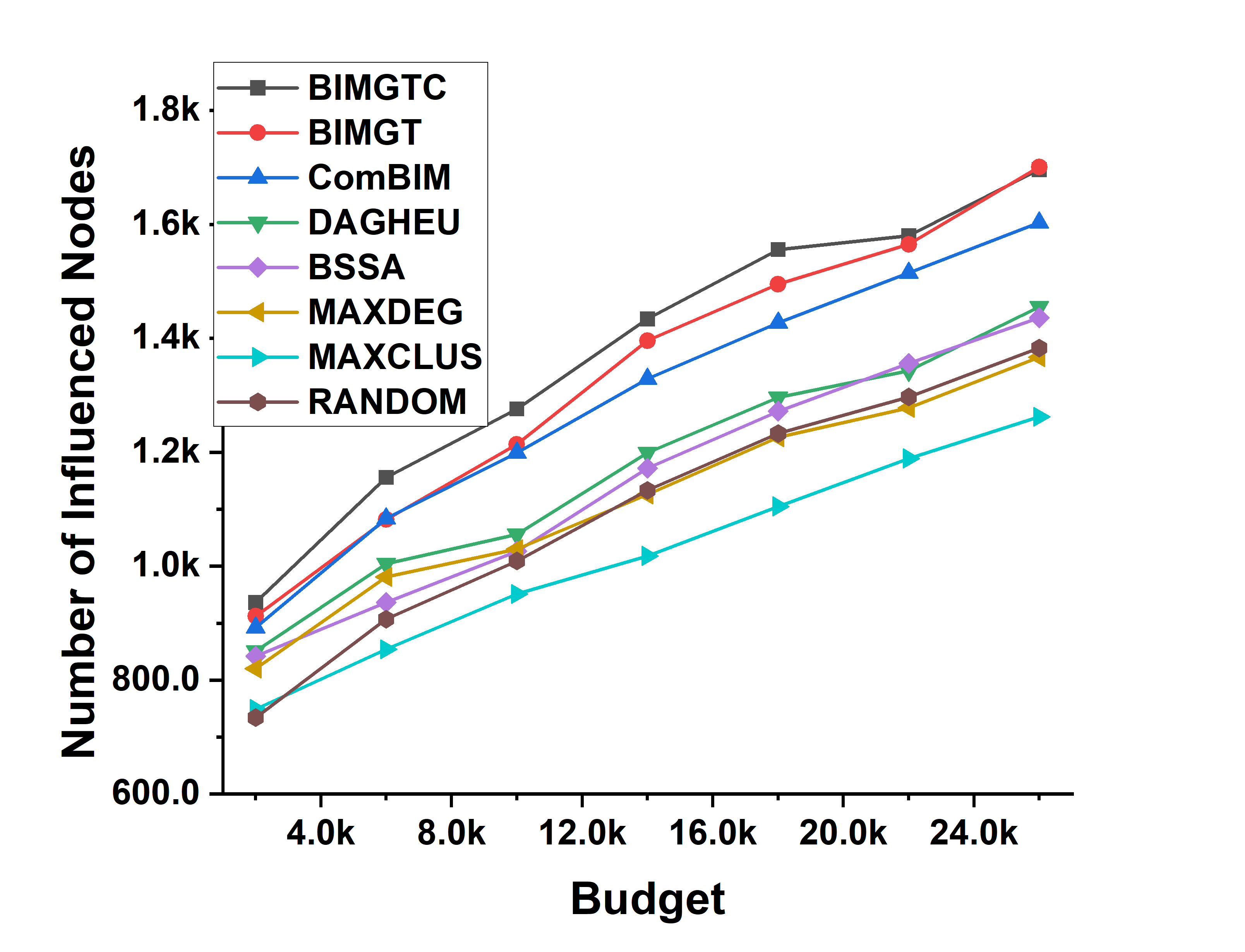
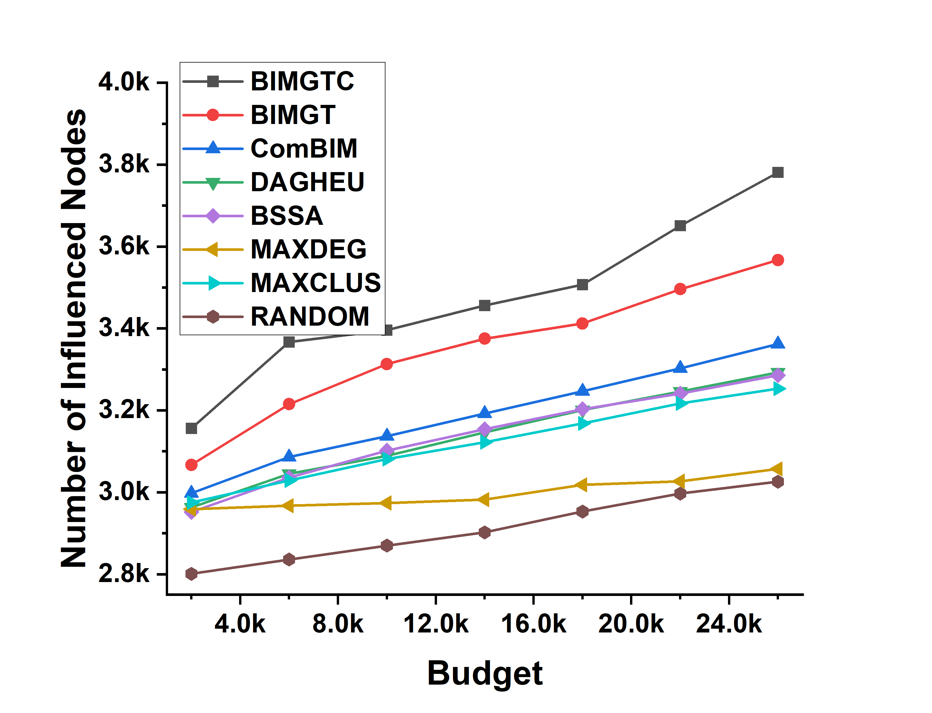
(a) CMP Dataset ($p_{c}=0.1$)	(b) CMP Dataset ($p_{c}=0.2$)
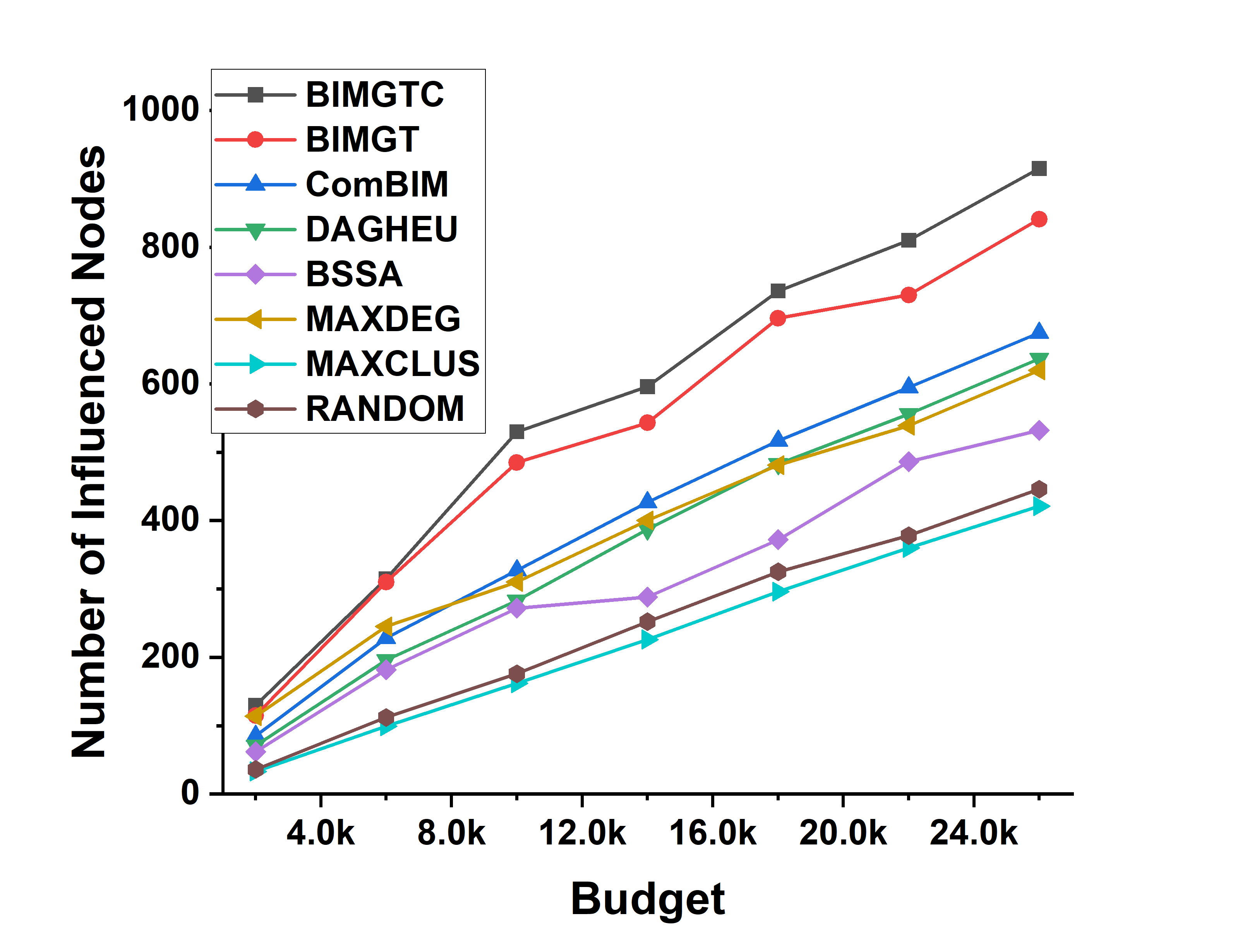
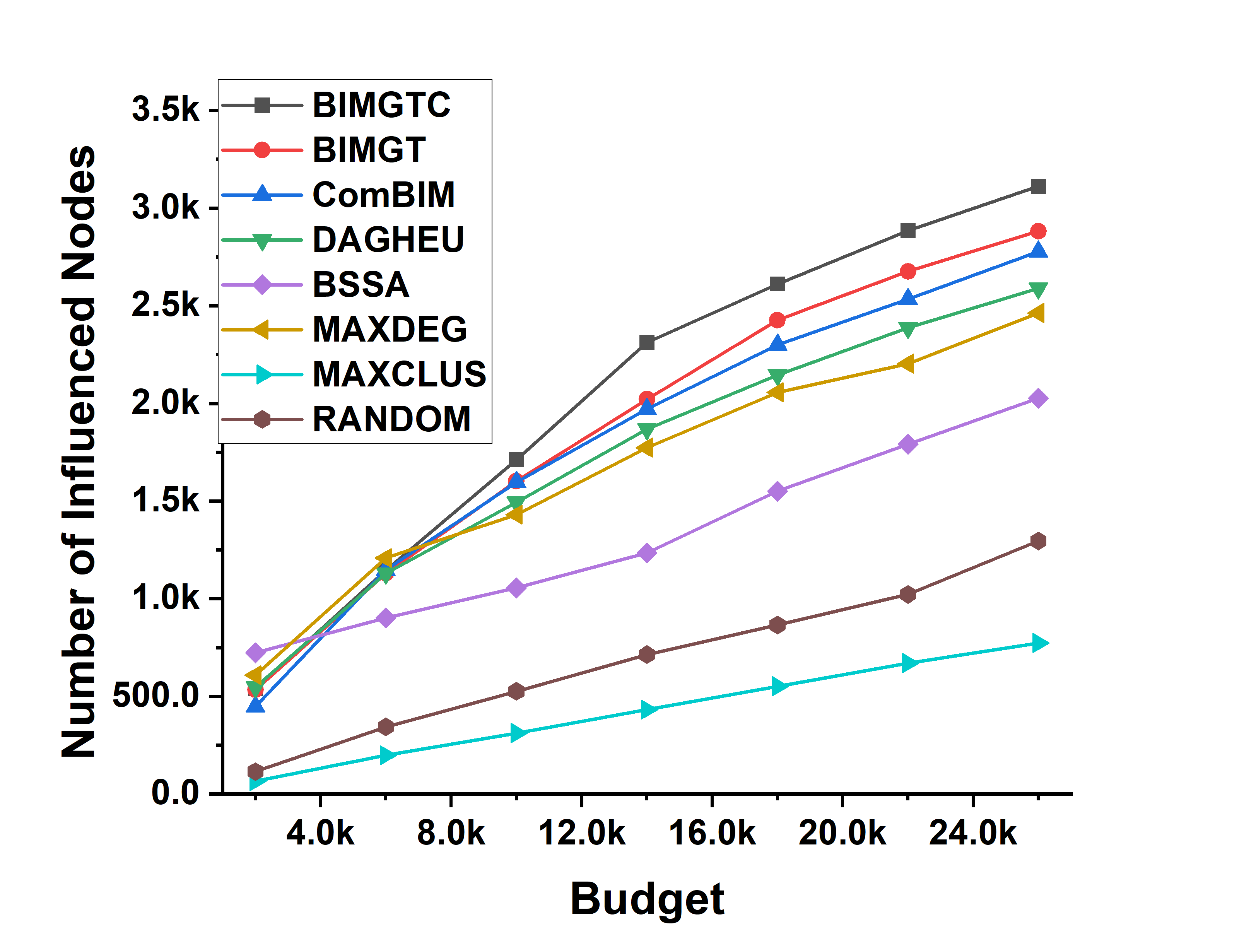
(c) CMP Dataset (Trivalancy)	(d) CMP Dataset (Weighted Cascade)

Figure 1: Budget Vs. Number of Influence Plots for the Collab2 dataset under the Uniform (with $p_{c}=0.1$ and $0.2$), Trivalency, Weighted Cascade and Count Probability settings.

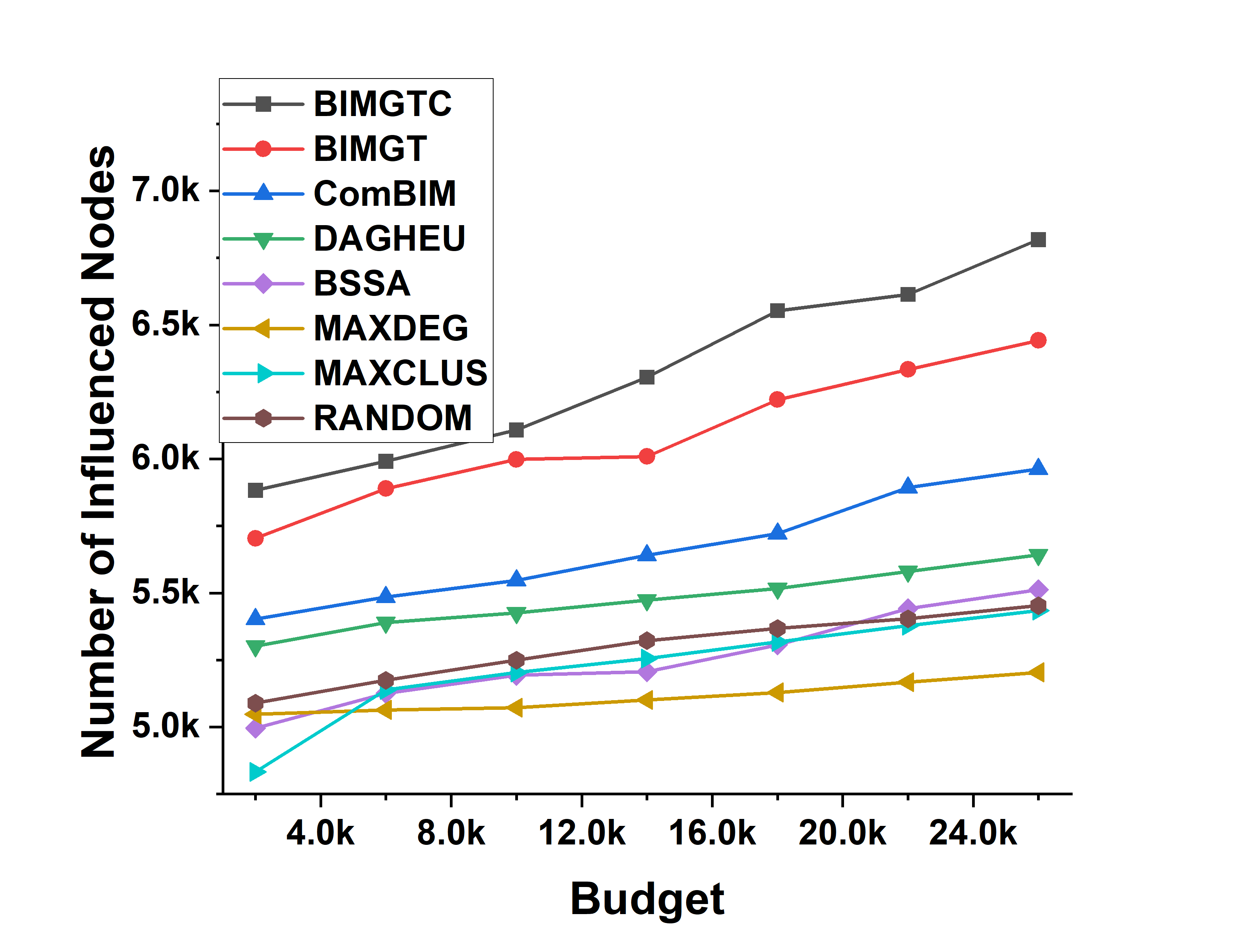
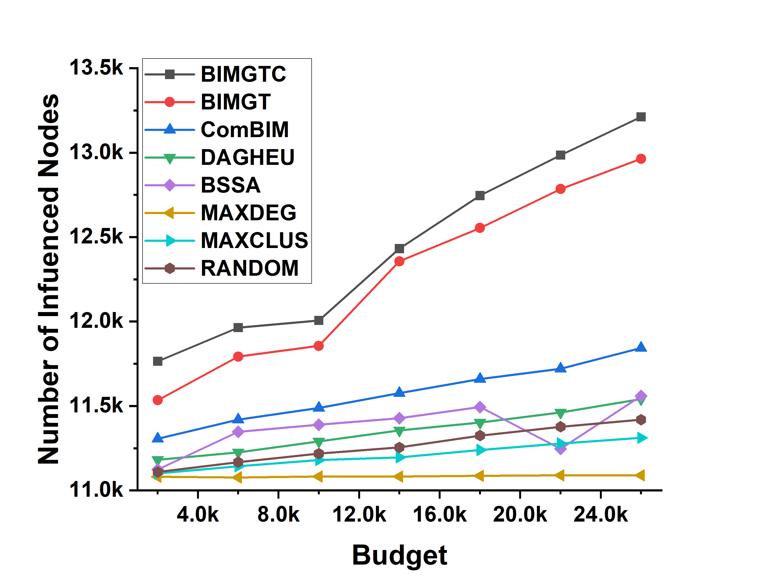
(a) CMP Dataset ($p_{c}=0.1$)	(b) CMP Dataset ($p_{c}=0.2$)
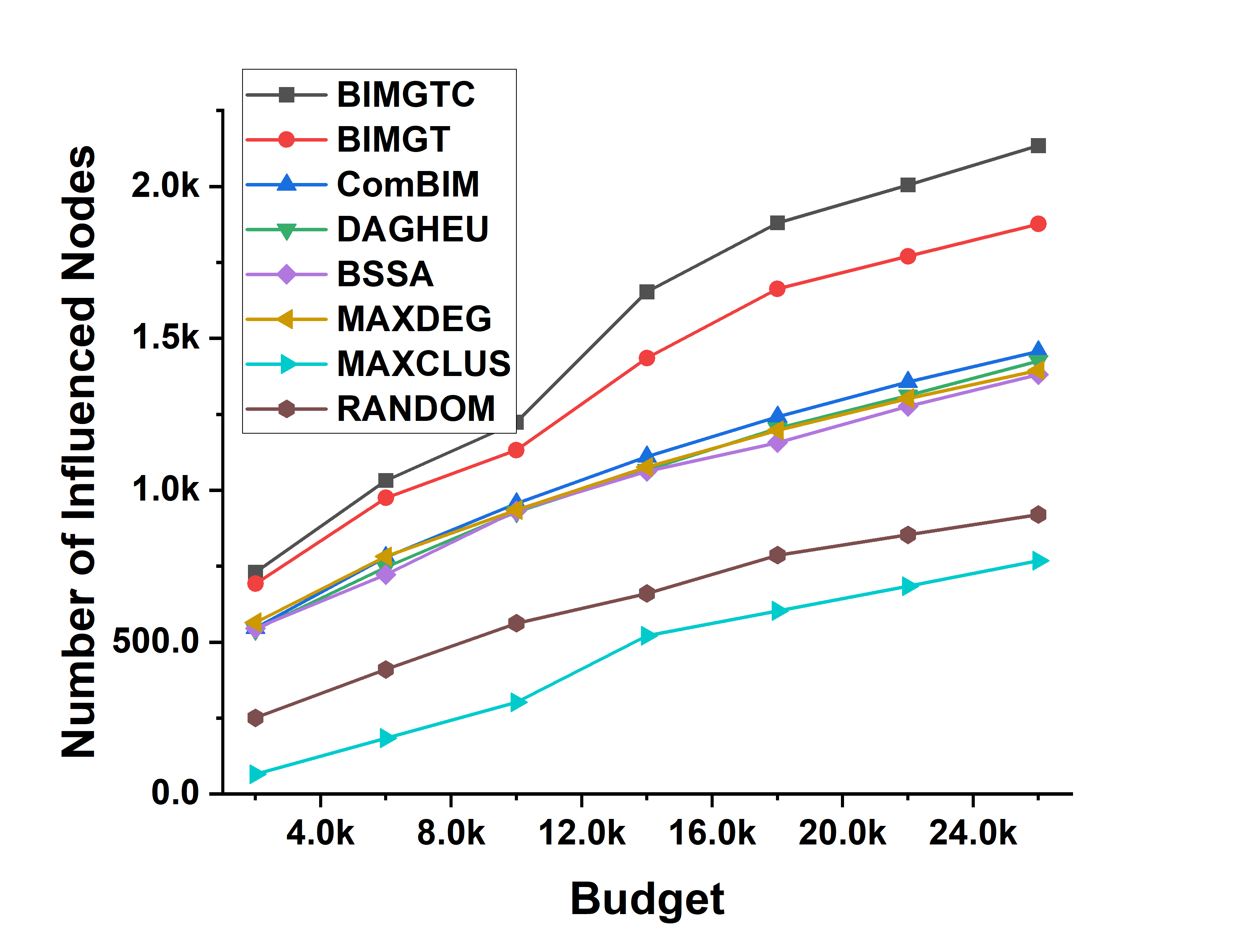
(c) CMP Dataset (Trivalancy)	(d) CMP Dataset (Weighted Cascade)

Figure 2: Budget Vs. Number of Influence Plots for the CMP Dataset dataset under the Uniform (with $p_{c}=0.1$ and $0.2$), Trivalency, Weighted Cascade and Count Probability settings.

Next, we describe the obtained results for the CMP Dataset. Figure 2 shows the budget vs. number of influenced nodes plot for the CMP Dataset. Like HEPT Dataset, in this dataset also the seed set selected by the proposed methodologies leads to the more number of influenced nodes compared to the existing methods. Here, we give an example. Under uniform probability setting when all the edges of the network have the influence probability of $0.2$, the seed set selected by the BIMGTC method leads to more number of influence nodes which is $13212$, which is almost $57.17\%$ of the network. Among the existing methods, ComBIM leads to a seed set that results to $11844$ number of influenced nodes, which is $51.2\%$. Hence, there is a gap of almost $6\%$ in terms of influence coverage. It is also important to observe that in this dataset also exploitation of the community structure leads to more amount of influenced nodes for the proposed methodology. As an example, for $\mathcal{B}=26000$ under the uniform probability setting with $p_{c}=0.2$, the seed set selected by BIMGT and BIMGTC leads to $12964$ and $13212$ number of influenced nodes, which is almost $1.9\%$ more.

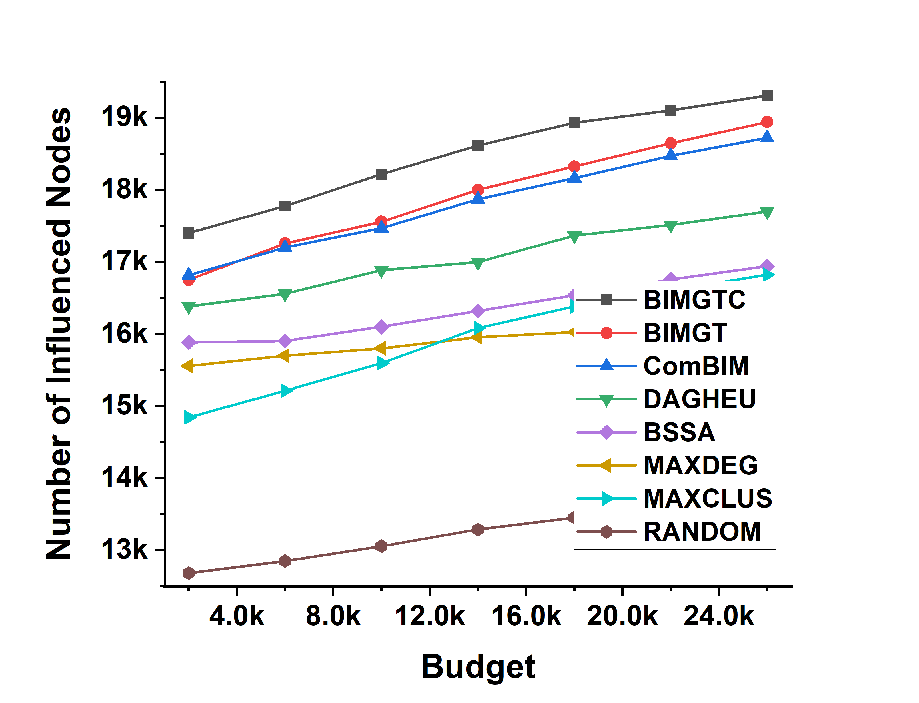
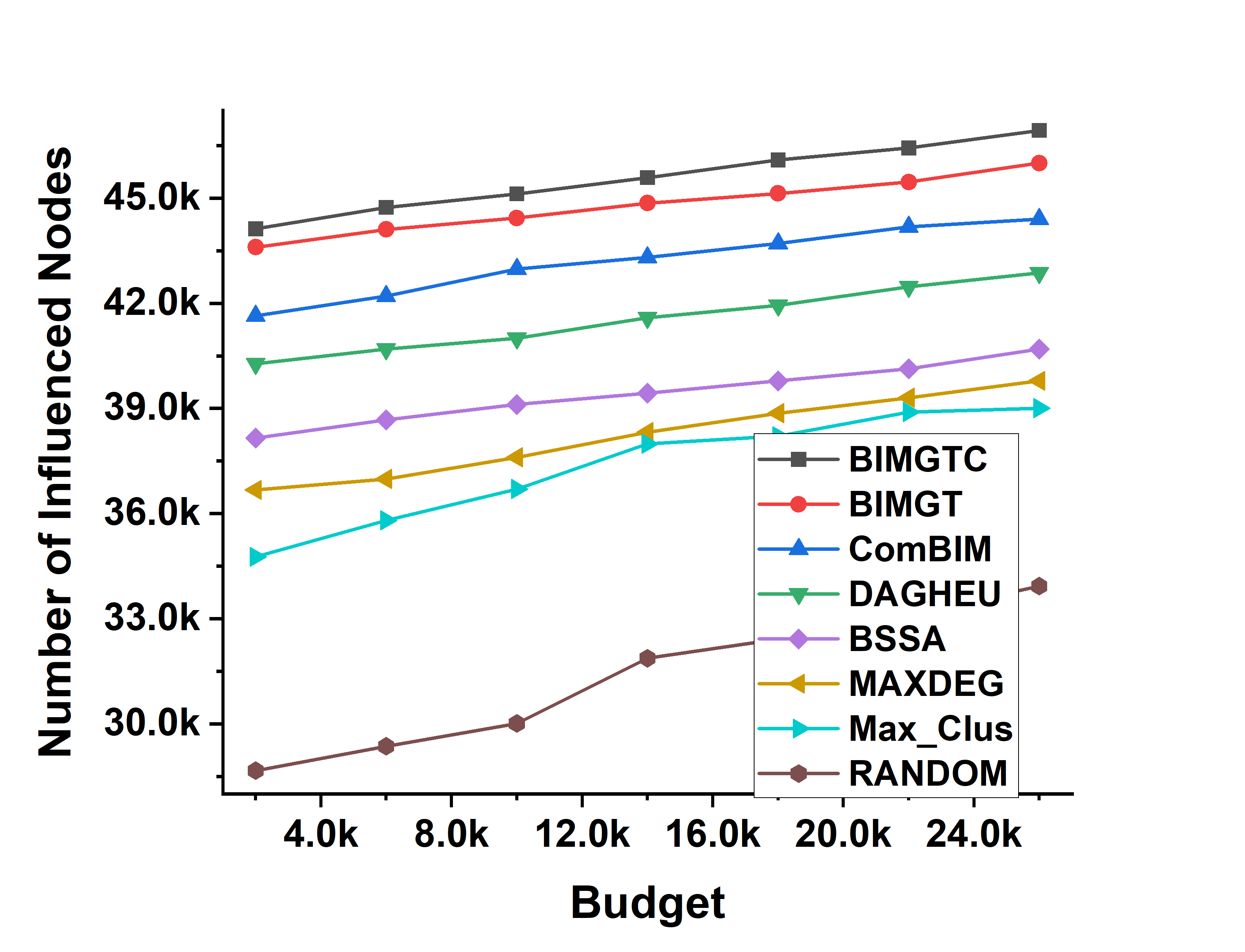
(a) Epinions ($p_{c}=0.1$)	(b) Epinions ($p_{c}=0.2$)
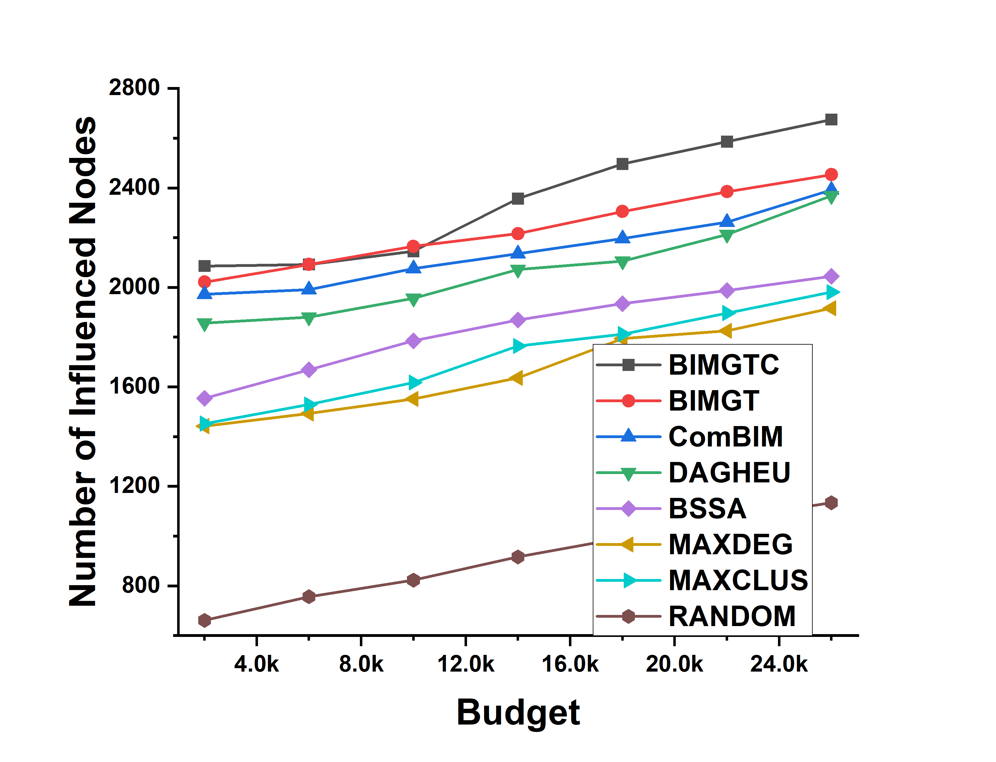
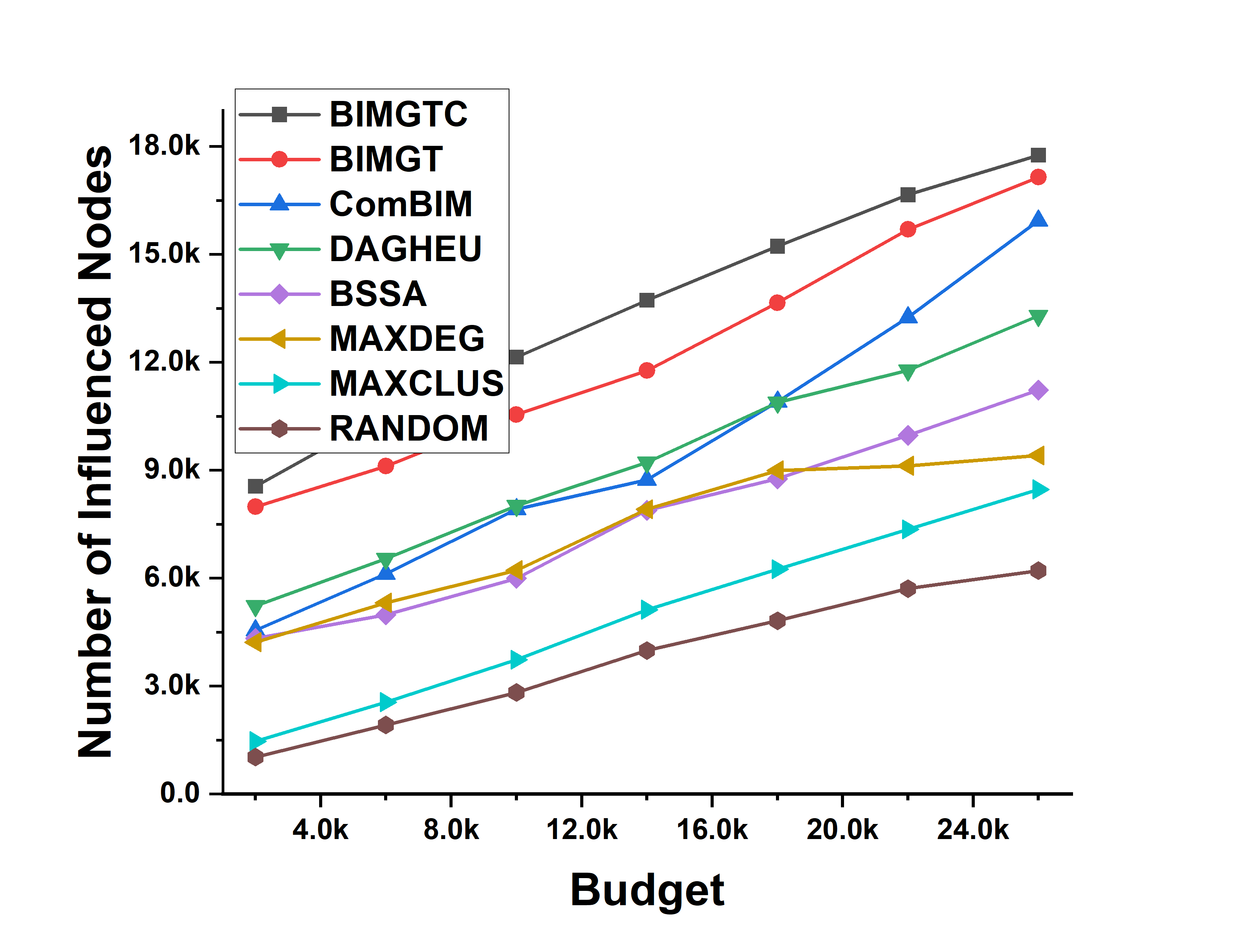
(d) Epinions (Trivalancy)	(e) Epinions (Weighted Cascade)

Figure 3: Budget Vs. Number of Influence Plots for the Epinions dataset under the Uniform (with $p_{c}=0.1$ and $0.2$), Trivalency, Weighted Cascade and Count Probability settings.

Figure 3 shows the budget vs. number of influenced nodes plot for the Epinions dataset. Like previous two datasets, in this dataset also we observe that the seed set selected by the proposed methodologies leads to the more number of influenced nodes compared to the baseline methods. As an example in case of uniform probability setting when $p_{c}=0.2$ and $\mathcal{B}=26000$, among the proposed methodologies the seed set selected by the BIMGTC leads to the maximum number of influenced nodes which is $46934$. On the other hand, among the existing methods the seed set selected by ComBIM leads to the maximum number of influenced nodes which is $44402$. From Table 2, it can be observed that the number of nodes of the Epinions dataset is $75879$. Hence, the percentage of nodes influenced by these seed nodes are $61.8\%$ and $58.5\%$, respectively. So, there is an approximate gap of $3.3\%$ in terms of expected influence. It is also important to observe that due to the exploitation of the community structure of the input network, the number of influenced nodes increases. As an example when $p_{c}=0.2$ and $\mathcal{B}=26000$, the number of influenced nodes by the seed set selected by BIMGTC and BIMGT are $46934$ and $45997$, respectively. Next, we proceed to discuss computational time requirement.

5.5.2 Computational Time

Table 3 shows the execution time of different algorithms for seed set selection. From this table it has been observed that the RANDOM takes the least amount of time across all the datasets. Next, MAXDEG takes more time than random as it needs to compute the degree of the nodes. MAXCLUS takes even more time than MAXDEG because computing clustering coefficient is much more computationally expensive operation than the degree. Remaining existing methods takes much more time than the baseline methods. It is important to observe that the computational time requirement of both the proposed methodologies are much less than that of the DAG-Based heuristic. It has been observed that the proposed methodologies takes more computational time compared to some of the baseline methods. However, it is important to realize that in many practical applications including viral marketing, computational advertisement etc., it is important to have an algorithm for seed set selection which has reasonable computational time with significant influence coverage. In this aspect, the proposed methodologies are far ahead compared to many existing methods.

Table 3: Computational time requirement (in Secs.) for seed set selection for HEP-THOY, COND-MAT and Epinions Dataset

Dataset	Budget	Algorithm
		BIMGTC	BIMGT	ComBIM	MAX_DEG	MAX_CLUS	RANDOM	BSSA	DAGHEU
HEP-THOY	2000	344	326	102	0.0464	0.3535	0.0032	22	1225
	6000	354	342	104	0.0488	0.3674	0.0085	26	1242
	10000	362	349	104	0.0483	0.3666	0.0092	24	1251
	14000	364	348	104	0.0497	0.3556	0.0192	23	1258
	18000	372	352	104	0.0492	0.3608	0.0269	25	1278
	22000	389	364	104	0.0503	0.3543	0.0333	28	1283
	26000	395	368	105	0.0496	0.3557	0.039	33	1299
COND-MAT	2000	810	785	345	0.0749	0.8999	0.0031	35	3640
	6000	812	796	344	0.0758	0.8964	0.0119	36	3676
	10000	824	810	344	0.0764	0.8968	0.0185	39	3697
	14000	835	826	344	0.0772	0.8979	0.0311	38	3723
	18000	846	832	349	0.0776	0.8981	0.0401	46	3761
	22000	858	844	349	0.0784	0.9004	0.0450	42	3800
	26000	866	852	350	0.0778	0.9034	0.0541	44	3866
Epinions	2000	1482	1456	1052	0.2649	199	0.0081	66	14620
	6000	1521	1490	1051	0.2758	201	0.0219	72	14751
	10000	1532	1506	1082	0.3821	226	0.0234	75	14762
	14000	1546	1523	1079	0.3422	225	0.0312	78	14463
	18000	1562	1540	1116	0.3776	238	0.0427	81	14561
	22000	1575	1556	1131	0.5261	231	0.0392	79	14600
	26000	1596	1574	1139	0.5116	229	0.0798	92	14786

6 Conclusion and Future Direction

In this paper, we have proposed a co-operative game theoretic framework for the budgeted influence maximization problem. Particularly, we formulate a co-operative game, where the users of the network are the players, and for any subset of the players, their utility is defined as the expected influence by the users of the subset under the MIA Model of diffusion. We have used the solution concept called ‘shapley value’ and proposed an iterative algorithm for selecting influential users in the network. We have also shown that the proposed methodology can select better quality seed set if the community structure of the network is exploited. Experiments with real-world social network datasets demonstrate the superiority of the proposed methodologies. Now, this study can be extended in different directions. First of all, we have not given any approximation guarantee of our proposed methodologies with respect to an optimal seed set. It will be interesting to come up with some worst case performance guarantee for our proposed methodologies. We have not considered the time-varying nature of the social network. There are many other solution concepts of co-operative game, such as Banzhaf index Dubey and Shapley [1979] etc. These solution concepts can be used instead of ‘shapley value’ and compare the performance with the proposed methodologies.

References

- Angell and Schoenebeck [2017] Angell, R., Schoenebeck, G., 2017. Don’t be greedy: Leveraging community structure to find high quality seed sets for influence maximization, in: International Conference on Web and Internet Economics, Springer. pp. 16–29.
- Aslay et al. [2015] Aslay, C., Lu, W., Bonchi, F., Goyal, A., Lakshmanan, L.V., 2015. Viral marketing meets social advertising: Ad allocation with minimum regret. Proceedings of the VLDB Endowment 8, 814–825.
- Banerjee et al. [2019] Banerjee, S., Jenamani, M., Pratihar, D.K., 2019. Combim: A community-based solution approach for the budgeted influence maximization problem. Expert Systems with Applications 125, 1–13.
- Banerjee et al. [2020] Banerjee, S., Jenamani, M., Pratihar, D.K., 2020. A survey on influence maximization in a social network. Knowledge and Information Systems , 1–39.
- Blondel et al. [2008] Blondel, V.D., Guillaume, J.L., Lambiotte, R., Lefebvre, E., 2008. Fast unfolding of communities in large networks. Journal of statistical mechanics: theory and experiment 2008, P10008.
- Borodin et al. [2010] Borodin, A., Filmus, Y., Oren, J., 2010. Threshold models for competitive influence in social networks, in: International workshop on internet and network economics, Springer. pp. 539–550.
- Bozorgi et al. [2016] Bozorgi, A., Haghighi, H., Zahedi, M.S., Rezvani, M., 2016. Incim: A community-based algorithm for influence maximization problem under the linear threshold model. Information Processing & Management 52, 1188–1199.
- Chen et al. [2010a] Chen, W., Liu, Z., Sun, X., Wang, Y., 2010a. A game-theoretic framework to identify overlapping communities in social networks. Data Mining and Knowledge Discovery 21, 224–240.
- Chen et al. [2010b] Chen, W., Wang, C., Wang, Y., 2010b. Scalable influence maximization for prevalent viral marketing in large-scale social networks, in: Proceedings of the 16th ACM SIGKDD international conference on Knowledge discovery and data mining, ACM. pp. 1029–1038.
- Chen et al. [2012] Chen, Y., Chang, S., Chou, C., Peng, W., Lee, S., 2012. Exploring community structures for influence maximization in social networks, in: The 6th SNA-KDD Workshop on Social Network Mining and Analysis Held in Conjunction with KDD, pp. 1–6.
- Chen et al. [2014] Chen, Y.C., Zhu, W.Y., Peng, W.C., Lee, W.C., Lee, S.Y., 2014. Cim: Community-based influence maximization in social networks. ACM Transactions on Intelligent Systems and Technology (TIST) 5, 25.
- Clark and Poovendran [2011] Clark, A., Poovendran, R., 2011. Maximizing influence in competitive environments: A game-theoretic approach, in: International Conference on Decision and Game Theory for Security, Springer. pp. 151–162.
- Cohen et al. [2014] Cohen, E., Delling, D., Pajor, T., Werneck, R.F., 2014. Sketch-based influence maximization and computation: Scaling up with guarantees, in: Proceedings of the 23rd ACM International Conference on Conference on Information and Knowledge Management, pp. 629–638.
- Cormen et al. [2009] Cormen, T.H., Leiserson, C.E., Rivest, R.L., Stein, C., 2009. Introduction to algorithms. MIT press.
- Ding et al. [2010] Ding, F., Liu, Y., Shen, B., Si, X.M., 2010. An evolutionary game theory model of binary opinion formation. Physica A: Statistical Mechanics and its Applications 389, 1745–1752.
- Domingos [2005] Domingos, P., 2005. Mining social networks for viral marketing. IEEE Intelligent Systems 20, 80–82.
- Domingos and Richardson [2001] Domingos, P., Richardson, M., 2001. Mining the network value of customers, in: Proceedings of the seventh ACM SIGKDD international conference on Knowledge discovery and data mining, ACM. pp. 57–66.
- Dubey and Shapley [1979] Dubey, P., Shapley, L.S., 1979. Mathematical properties of the banzhaf power index. Mathematics of Operations Research 4, 99–131.
- Goyal et al. [2011a] Goyal, A., Lu, W., Lakshmanan, L.V., 2011a. Celf++: optimizing the greedy algorithm for influence maximization in social networks, in: Proceedings of the 20th international conference companion on World wide web, ACM. pp. 47–48.
- Goyal et al. [2011b] Goyal, A., Lu, W., Lakshmanan, L.V., 2011b. Simpath: An efficient algorithm for influence maximization under the linear threshold model, in: 2011 IEEE 11th international conference on data mining, IEEE. pp. 211–220.
- Guille et al. [2013] Guille, A., Hacid, H., Favre, C., Zighed, D.A., 2013. Information diffusion in online social networks: A survey. ACM Sigmod Record 42, 17–28.
- Güney [2019] Güney, E., 2019. On the optimal solution of budgeted influence maximization problem in social networks. Operational Research 19, 817–831.
- HAFIENE et al. [2020] HAFIENE, N., KAROUI, W., ROMDHANE, L.B., 2020. Influential nodes detection in dynamic social networks: A survey. Expert Systems with Applications , 113642.
- Han et al. [2014] Han, S., Zhuang, F., He, Q., Shi, Z., 2014. Balanced seed selection for budgeted influence maximization in social networks, in: Pacific-Asia Conference on Knowledge Discovery and Data Mining, Springer. pp. 65–77.
- Hong and Liu [2019] Hong, T., Liu, Q., 2019. Seeds selection for spreading in a weighted cascade model. Physica A: Statistical Mechanics and its Applications 526, 120943.
- Hossain [2012] Hossain, M., 2012. Users’ motivation to participate in online crowdsourcing platforms, in: 2012 International Conference on Innovation Management and Technology Research, IEEE. pp. 310–315.
- Jung et al. [2012] Jung, K., Heo, W., Chen, W., 2012. Irie: Scalable and robust influence maximization in social networks, in: 2012 IEEE 12th International Conference on Data Mining, IEEE. pp. 918–923.
- Ke et al. [2018] Ke, X., Khan, A., Cong, G., 2018. Finding seeds and relevant tags jointly: For targeted influence maximization in social networks, in: Proceedings of the 2018 International Conference on Management of Data, pp. 1097–1111.
- Kempe et al. [2003] Kempe, D., Kleinberg, J., Tardos, É., 2003. Maximizing the spread of influence through a social network, in: Proceedings of the ninth ACM SIGKDD international conference on Knowledge discovery and data mining, ACM. pp. 137–146.
- Kempe et al. [2005] Kempe, D., Kleinberg, J., Tardos, É., 2005. Influential nodes in a diffusion model for social networks, in: International Colloquium on Automata, Languages, and Programming, Springer. pp. 1127–1138.
- Kempe et al. [2015] Kempe, D., Kleinberg, J.M., Tardos, É., 2015. Maximizing the spread of influence through a social network. Theory of Computing 11, 105–147. URL: https://doi.org/10.4086/toc.2015.v011a004, doi:10.4086/toc.2015.v011a004.
- Kostka et al. [2008] Kostka, J., Oswald, Y.A., Wattenhofer, R., 2008. Word of mouth: Rumor dissemination in social networks, in: International colloquium on structural information and communication complexity, Springer. pp. 185–196.
- Leskovec et al. [2007a] Leskovec, J., Kleinberg, J., Faloutsos, C., 2007a. Graph evolution: Densification and shrinking diameters. ACM Transactions on Knowledge Discovery from Data (TKDD) 1, 2.
- Leskovec et al. [2007b] Leskovec, J., Krause, A., Guestrin, C., Faloutsos, C., Faloutsos, C., VanBriesen, J., Glance, N., 2007b. Cost-effective outbreak detection in networks, in: Proceedings of the 13th ACM SIGKDD international conference on Knowledge discovery and data mining, ACM. pp. 420–429.
- Li et al. [2015] Li, H., Bhowmick, S.S., Cui, J., Gao, Y., Ma, J., 2015. Getreal: Towards realistic selection of influence maximization strategies in competitive networks, in: Proceedings of the 2015 ACM SIGMOD international conference on management of data, pp. 1525–1537.
- Li et al. [2017] Li, M., Wang, X., Gao, K., Zhang, S., 2017. A survey on information diffusion in online social networks: Models and methods. Information 8, 118.
- Li et al. [2018] Li, Y., Fan, J., Wang, Y., Tan, K.L., 2018. Influence maximization on social graphs: A survey. IEEE Transactions on Knowledge and Data Engineering 30, 1852–1872.
- Logins and Karras [2019] Logins, A., Karras, P., 2019. Content-based network influence probabilities: Extraction and application, in: 2019 International Conference on Data Mining Workshops (ICDMW), IEEE. pp. 69–72.
- Maleki et al. [2013] Maleki, S., Tran-Thanh, L., Hines, G., Rahwan, T., Rogers, A., 2013. Bounding the estimation error of sampling-based shapley value approximation. arXiv preprint arXiv:1306.4265 .
- Narahari [2014] Narahari, Y., 2014. Game theory and mechanism design. volume 4. World Scientific.