Non-dimensional parameters for the flapping dynamics of multilayered plates

Abstract

The coupled flow-induced flapping dynamics of flexible plates in uniform axial flows are governed by three non-dimensional numbers, namely: Reynolds number $(Re)$, mass-ratio $(m^{*})$, and non-dimensional flexural rigidity $(K_{B})$. The traditional definition of these parameters is limited to isotropic single-layered flexible plates. However, there is a need to define these parameters for a more generic plate of multiple isotropic layers placed on top of each other. In this work, we derive the non-dimensional parameters for a flexible plate of $n$-isotropic layers and validate the non-dimensional parameters with numerical simulations. The proposed non-dimensional framework connects the experimental, numerical, and analytical studies on single-layered plates with the flapping dynamics of multilayered plates.

[inst1]organization=Computing Lab, Department of Mechanical Engineering,addressline=Birla Institute of Technology and Science - Pilani, Hyderabad Campus, city=Secunderabad, postcode=500078, state=Telangana, country=India

[inst2]organization=Department of Mechanical Engineering,addressline=Birla Institute of Technology and Science - Pilani, K. K. Birla Goa Campus, city=Sancoale, postcode=403726, state=Goa, country=India

Piezoelectric patches used for energy harvesting are usually multilayered.

Non-dimensional parameters for flapping instability of flexible multilayered plates.

Analytical derivation of equivalent flexural rigidity and equivalent mass ratio.

1 Introduction

Fluid-structure interaction is a classical research area to investigate the effect of fluid flow on structures that can either move or deform and would in turn affect the fluid flow itself. Such interactions are omnipresent in nature (for example, the flapping of wings in avian animals and the fluttering of leaves) as well as engineering applications dealing with vortex-induced vibrations (VIV) [1, 2] and bio-medicine [3]. More recently, the problem of fluid-structure interactions has attracted substantial interest for its ability to harvest fluid kinetic energy into electrical energy. Electric energy is harvested from the vortex-induced vibrations (VIV) of circular cylinders as an ongoing research topic via piezoelectric [4, 5, 6, 7] and electromagnetic [8, 9, 10, 11] effects. Apart from bluff bodies, the interaction of streamline bodies such as rigid foils and flexible plates [12] with the incoming flow can be broadly categorized into propulsion [13, 14, 15, 16, 17] and energy extraction regimes [18, 19, 20, 21, 22].

Among the energy-harvesting alternatives, it has been noted that the maximum energy density of a piezoelectric transducer is around 63 and 8 times more than that of electrostatic and electromagnetic transducers, respectively [23]. Furthermore, piezoelectric conversion has benefits such as high transmission efficiency and the least complex and economical design. An Eel-like device manufactured from polyvinylidene fluoride (PVDF) was utilized to harvest energy using ocean waves. It used a trail of traveling vortices behind a bluff body to strain piezoelectric elements for power generation [18, 24]. Similarly, a piezoelectric tree composed of a flexible and conducting leaf structure around a central “trunk” made of PVDF was used to harvest wind energy [25]. Wind-induced vibrations lead to the deformation of the piezoelectric material, which results in the generation of electric current. Unlike rigid structures, modeling the flow across flexible structures is challenging numerically and experimentally. The strain energy of the flexible structure performing the flapping motion is converted into electrical energy via a piezoelectric mechanism in energy harvesting devices, which adds to the complexity of the modeling. Investigations have been conducted to optimize the energy output from such piezoelectric harvesting devices by studying the resonant conditions [26], flow orientation, plate orientation [27, 28, 29, 30] and electrode position [31]. In these experiments, it is common for the piezoelectric materials to be mounted on thicker plate-like structures made of materials such as Mylar [26] or polyurethane [18], thereby resulting in a multilayered flexible structure for energy harvesting. Various numerical methods based on the finite difference method [32, 33], finite element method [34, 28] and lattice Boltzmann method [35, 36], have been used to investigate the non-linear two/three-dimensional flow induced flapping response, force and vortex dynamics to understand the physics behind the flapping phenomena for isotropic flexible structures.

Even though piezoelectric energy harvesting devices are multilayered, the current understanding of the non-linear flapping dynamics is limited to results from isotropic models. An attempt was made earlier by Akcabay and Young [20], where the flapping dynamics of a three-layered flexible plate were numerically investigated by considering an equivalent single-layered plate’s Young’s modulus for the three-layered flexible plate. More recently, in Saravanakumar et al. [37], a quasi-monolithic formulation was considered to numerically investigate the post-critical flapping dynamics of a two-layered plate in a uniform flow. The study revealed that variation in material properties across the layers could result in complex flapping dynamics. Hence, there is a crucial need for developing non-dimensional parameters that can generalize the flapping dynamics of multilayered structures.

Building upon the work of Saravanakumar et al. [37], the current study aims at formulating the equivalent, non-dimensional mass ratio and flexural rigidity for an n-layered plate. Therefore, it lays the groundwork for a complete description of the flapping dynamics for multilayered plates. The following formulation simplifies the analysis of a system by reducing the number of variables and parameters involved. According to the knowledge of the authors, although multilayered plates are extensively used in engineering, there does not exist a non-dimensional framework to describe the physics of such sandwiched structures undergoing flapping due to interaction with the surrounding flow. Therefore, this generalized novel description of multilayered plates will be imperative for their experimental, numerical and analytical analyses.

The layout of the article is as follows. The non-dimensional parameters are derived and constructed for the multilayered plates in Section 2. The generalized description is then systematically verified by considering multiple case scenarios in Section 3. The study is summarized and concluded in Section 4.

2 Construction of Non-dimensional Parameters

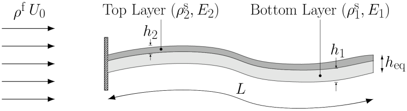
(a) Side view

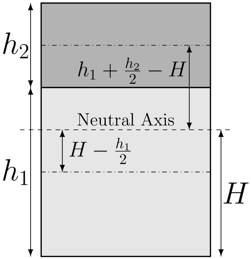
(b) Cross-sectional view

Figure 1: A schematic of a two-layered flexible plate, with a fixed leading edge, flapping in a uniform stream.

In this section, we present an analytical derivation for the non-dimensional parameters that govern the self-sustained flapping dynamics of multilayered plates. Initially, we construct the non-dimensional parameters for a two-layered plate and then generalize the derivation for the case of an $n$-layered plate. The flapping dynamics of a single-layered isotropic flexible plate are relatively well understood and are known to depend on the structure to fluid mass-ratio ($m^{*}$), non-dimensional flexural rigidity ($K_{B}$) and Reynolds number ($Re$) [38, 33, 39] which are defined as

$$m^{*}=\frac{\rho^{\mathrm{s}}h}{\rho^{\mathrm{f}}L}\qquad K_{B}=\frac{B}{\rho^{\mathrm{f}}U_{0}^{2}L^{3}}\qquad Re=\frac{\rho^{\mathrm{f}}U_{0}L}{\mu^{\mathrm{f}}},$$ (1)

where $B$ and $\rho^{\mathrm{s}}$ represent the flexural rigidity and density of the flexible plate, respectively, and $\mu^{\mathrm{f}}$ is the dynamic viscosity of the fluid. These definitions can be extended for multilayered flexible plates by modifying the non-dimensional parameters, $m^{*}$, and $K_{B}$, to replace the properties of the single-layered plate such as $\rho^{\mathrm{s}}$, $h$ and $B$ with their equivalent values for a multilayered plate.

Figure 1 shows a representative schematic of a two-layered flexible plate of length $L$ and thickness $h_{\mathrm{eq}}$ flapping about its leading edge. The flexible plate interacts with a uniform incompressible viscous fluid of density $\rho^{\mathrm{f}}$, flowing along its length at a flow velocity of $U_{0}$. In this work, $\left(\rho^{\mathrm{s}}_{1},E_{1},\nu_{1},h_{1}\right)$ and $\left(\rho^{\mathrm{s}}_{2},E_{2},\nu_{2},h_{2}\right)$ represent the density, Young’s modulus, Poisson’s ratio and thickness of the bottom and top layers, respectively. The total thickness of the two-layered plate is given as $h_{\mathrm{eq}}=h_{1}+h_{2}$.

The structural dynamics of the flapping plate are described by the Euler-Bernoulli beam equation given as

$$\rho_{\mathrm{eq}}^{\mathrm{s}}h_{\mathrm{eq}}\frac{\partial^{2}w}{\partial t^{2}}+B_{\mathrm{eq}}\frac{\partial^{4}w}{\partial x^{4}}=f,$$ (2)

where $\rho_{\mathrm{eq}}^{\mathrm{s}}$ and $B_{\mathrm{eq}}$ represent the equivalent density and equivalent flexural rigidity for the combined two-layered plate. Here, $w$ denotes the transverse deflection of the plate due to the fluid loading $f$ acting on the plate. The equivalent density $\rho_{\mathrm{eq}}^{\mathrm{s}}$ and equivalent flexural rigidity $B_{\mathrm{eq}}$ are defined as

$$\rho_{\mathrm{eq}}^{\mathrm{s}}=\frac{\rho^{\mathrm{s}}_{1}h_{1}+\rho^{\mathrm{s}}_{2}h_{2}}{h_{\mathrm{eq}}}\quad B_{\mathrm{eq}}=\frac{E_{1}I_{1}}{(1-\nu_{1}^{2})}+\frac{E_{2}I_{2}}{(1-\nu_{2}^{2})}.$$ (3)

In Eq. 3, $I_{1}$ and $I_{2}$ represent the area moment of inertia for the bottom and top layers, respectively, calculated with respect to the neutral axis of the combined two-layered plate. For an isotropic plate with a uniform cross-section, the neutral axis will always pass through the centroid of the plate’s cross-section. However, for a two-layered or multilayered plate, the neutral axis may not pass through the centroid of the cross-section as its position depends on the thickness and Young’s modulus of each layer. In such cases, the position of the neutral axis can be determined by considering the stress equilibrium condition in the streamwise direction at any cross-section. For the case of pure bending in a two-layered plate, the equilibrium condition can be formulated as

$$\Sigma F_{\mathrm{x}}=\int_{A}\sigma_{\mathrm{x}}dA=0$$ (4)

$$-\int_{0}^{h_{1}}E_{1}\frac{(y-H)}{\gamma}~{}{b}~{}dy-\int_{h_{1}}^{h_{1}+h_{2}}E_{2}\frac{(y-H)}{\gamma}~{}{b}~{}dy=0,$$ (5)

where $\sigma_{\mathrm{x}}$, $\gamma$, ${b}$ and $H$ represent the normal stress along the streamwise direction, the plate width, the radius of curvature and the distance of the neutral axis from the bottom of the plate, respectively. Eq. 5 can be solved to deduce the expression for the position of a neutral axis $H$ as

$$H=\frac{E_{1}h_{1}\left({h_{1}}/{2}\right)+E_{2}h_{2}\left(h_{1}+{h_{2}}/{2}\right)}{(E_{1}h_{1}+E_{2}h_{2})}.$$ (6)

The parallel axis theorem can then be used to calculate the area moments of inertia $I_{1}$ and $I_{2}$ about the neutral axis (see Fig. 1). The resulting expressions are

$$I_{1}=\frac{h_{1}^{3}}{12}+h_{1}\left(\frac{h_{1}}{2}-H\right)^{2}\hskip 14.22636ptI_{2}=\frac{h_{2}^{3}}{12}+h_{2}\left(h_{1}+\frac{h_{2}}{2}-H\right)^{2}.$$ (7)

Upon substituting these expressions in Eq. 3, we obtain the final form of the equation for the equivalent flexural rigidity ($B_{\mathrm{eq}}$) as

$$\begin{split}B_{\mathrm{eq}}&=\frac{E_{1}}{(1-\nu_{1}^{2})}\left[\frac{h_{1}^{3}}{12}+h_{1}\left(\frac{h_{1}}{2}-H\right)^{2}\right]+\frac{E_{2}}{(1-\nu_{2}^{2})}\left[\frac{h_{2}^{3}}{12}+h_{2}\left(h_{1}+\frac{h_{2}}{2}-H\right)^{2}\right]\end{split}$$ (8)

Finally, the modified mass-ratio $m^{*}_{\mathrm{eq}}$ and non-dimensional flexural rigidity $K_{B}^{\mathrm{eq}}$ that govern the flapping dynamics of a two-layered flexible plate are defined as

$$m^{*}_{\mathrm{eq}}=\frac{\rho^{\mathrm{s}}_{\mathrm{eq}}h_{\mathrm{eq}}}{\rho^{\mathrm{f}}L}\qquad K_{B}^{\mathrm{eq}}=\frac{B_{\mathrm{eq}}}{\rho^{\mathrm{f}}U_{0}^{2}L^{3}}.$$ (9)

Furthermore, the expressions for $H$ and $B_{\mathrm{eq}}$ in Eqs. 6 and 8, respectively, for the case of a two-layered plate can be generalized for a $n$-layered plate following the same equilibrium condition approach as

$$H=\frac{E_{1}h_{1}\left({h_{1}}/{2}\right)+\cdots+E_{n}h_{n}\left(h_{1}+\cdots+h_{n-1}+h_{n}/2\right)}{(E_{1}h_{1}+E_{2}h_{2}+\cdots+E_{n-1}h_{n-1}+E_{n}h_{n})}$$

$$H=\frac{\sum_{i=1}^{n}\left[E_{i}h_{i}\left(\sum_{j=1}^{i}h_{j}-\frac{h_{i}}{2}\right)\right]}{\sum_{i=1}^{n}E_{i}h_{i}}\$$ (10)

$$B_{\mathrm{eq}} = \frac{E_{1}}{(1-\nu_{1}^{2})}\left[\frac{h_{1}^{3}}{12}+h_{1}\left(\frac{h_{1}}{2}-H\right)^{2}\right]+\frac{E_{2}}{(1-\nu_{2}^{2})}\left[\frac{h_{2}^{3}}{12}+h_{2}\left(h_{1}+\frac{h_{2}}{2}-H\right)^{2}\right]+\cdots$$ (11)

$$+ \frac{E_{n}}{(1-\nu_{n}^{2})}\left[\frac{h_{n}^{3}}{12}+h_{n}\left(h_{1}+\cdots+h_{n-1}+\frac{h_{n}}{2}-H\right)^{2}\right]$$

$$B_{\mathrm{eq}}=\sum_{i=1}^{n}\frac{E_{i}}{1-\nu^{2}_{i}}\left[\frac{h^{3}_{i}}{12}+h_{i}\left(\sum_{j=1}^{i}h_{j}-\frac{h_{i}}{2}-H\right)^{2}\right]$$ (12)

We can use these definitions to define the non-dimensional parameters for a $n$-layered plate, according to Eq. 9. It is noteworthy that although the equivalent mass ratio is the linear summation of the independent mass ratios of each layer, the equivalent non-dimensional flexural rigidity is not equal to the sum of the independent non-dimensional flexural rigidity of each layer.

3 Numerical Verification

The newly proposed non-dimensional parameters were validated by conducting ten parametric numerical experiments to simulate the flapping dynamics of a two-layered plate placed in a uniform stream for $Re=1000$. Table 1 provides the material properties of the ten cases that can be further divided into two sets. Set-I consists of the first five cases from Table 1 which will validate the equivalent flexural rigidity $K_{B}^{\mathrm{eq}}$. Here the values of $m_{\mathrm{1}}^{*}$, $m_{\mathrm{2}}^{*}$ and $m_{\mathrm{eq}}^{*}$ are kept constant and equal to 0.1. For cases 1 and 2, the parameters $K_{\mathrm{B}}^{1}$ and $K_{\mathrm{B}}^{2}$ are selected such that $K_{\mathrm{B}}^{eq}$ for both cases is equal to 0.0005. Similarly, different values of $K_{\mathrm{B}}^{1}$ and $K_{\mathrm{B}}^{2}$ are chosen for cases 3 and 4 such that the resultant $K_{\mathrm{B}}^{eq}$ is 0.0004. In order to validate the effect of the thickness of the layers on the non-dimensional parameters, cases 1 to 4 are constructed by assuming the thickness of the top layer is the same as that of the bottom layer i.e. $h_{1}=h_{2}=0.005L$ and case 5 is constructed by choosing non-equal thicknesses for the individual layers. Set-II comprises cases 6 to 10 that validate the equivalent mass ratio $m^{*}_{\mathrm{eq}}$. The values of $K_{\mathrm{B}}^{1}$, $K_{\mathrm{B}}^{2}$ and $K_{\mathrm{B}}^{eq}$ are kept constant and equal to 0.0001 for the full set. For cases 6 and 7, the parameters $m_{\mathrm{1}}$ and $m_{\mathrm{2}}$ are selected such that $m^{*}_{\mathrm{eq}}$ is equal to 0.075 for both cases. Similarly, different values of $m_{\mathrm{1}}$ and $m_{\mathrm{2}}$ are chosen for cases 8, 9, and 10 such that the resultant $m^{*}_{\mathrm{eq}}$ remains 0.05 for all three cases. Similar to Set-I, cases 6 to 9 assume that the thickness of the top and the bottom layers remain identical and equal to $0.005L$ and case 10 presents the condition of layers with different thicknesses.

Table 1: Summary of governing parameters considered for the numerical validation.

Case	$\frac{\rho_{1}^{\mathrm{s}}}{\rho^{\mathrm{f}}}$	$\frac{\rho_{2}^{\mathrm{s}}}{\rho^{\mathrm{f}}}$	$m_{\mathrm{eq}}^{*}$	$h_{1}$	$h_{2}$	$\frac{E_{1}}{\rho^{\mathrm{f}}U_{0}^{2}\left(1-\nu_{1}^{2}\right)}$	$\frac{E_{2}}{\rho^{\mathrm{f}}U_{0}^{2}\left(1-\nu_{2}^{2}\right)}$	$K_{B}^{\mathrm{eq}}$
1	10.0	10.0	0.01	0.005	0.005	27761.5	1641.8	0.0005
2	10.0	10.0	0.01	0.005	0.005	6000.0	6000.0	0.0005
3	10.0	10.0	0.01	0.005	0.005	4800.0	4800.0	0.0004
4	10.0	10.0	0.01	0.005	0.005	28560.4	775.8	0.0004
5	10.0	10.0	0.01	0.0025	0.0075	778.5	10000.0	0.0004
6	10.0	5.0	0.075	0.005	0.005	1200.0	1200.0	0.0001
7	12.5	2.5	0.075	0.005	0.005	1200.0	1200.0	0.0001
8	5.0	5.0	0.05	0.005	0.005	1200.0	1200.0	0.0001
9	7.5	2.5	0.05	0.005	0.005	1200.0	1200.0	0.0001
10	12.5	2.5	0.05	0.0025	0.0075	1200.0	1200.0	0.0001

3.1 Computational setup

The interactions of the plate with the fluid flow are simulated using an in-house finite element based solver with exact interaction tracking presented in [37]. The computational setup shown in Fig. 2 consists of a two-layered flexible plate clamped at the leading edge. The trailing edge is left free to undergo self-induced flapping due to interaction with a uniform axial flow. The computational domain considered for the study is of the size $24L\times 10L$, wherein $L$ is the length of the plate. Considering that the fluid flows from left to right, a free stream velocity of $U_{0}$ enters the computation domain through $\Gamma^{f}_{in}$ and leaves through $\Gamma^{f}_{out}$. Accordingly, a traction-free boundary condition is placed on the outlet ($\Gamma^{f}_{out}$) of the computational domain. The top ($\Gamma^{f}_{top}$) and bottom ($\Gamma^{f}_{bottom}$) limits of the computational domain are bounded by the free-slip boundary condition. A no-slip boundary condition is imposed on the plate-fluid interface. The solver is $2^{\mathrm{nd}}$ order accurate in time and $3^{\mathrm{rd}}$ order accurate in space. As per the mesh convergence study carried out earlier [37], an identical high-order $\mathbb{P}_{2}$ finite element computational mesh has been selected. The mesh shown in Fig. 3 consists of 29549 nodes and 14657 $\mathbb{P}_{2}$ elements.

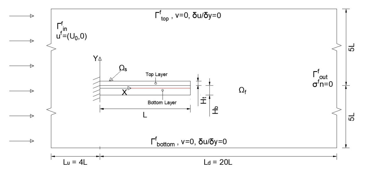
Figure 2: In the computational setup presented here, we can see the two-layered flexible plate in a uniform flow of velocity $U_{0}$, the boundary conditions and the interface separating the fluid domain from the solid domain. The dashed line (—) indicates the neutral surface of the plate.

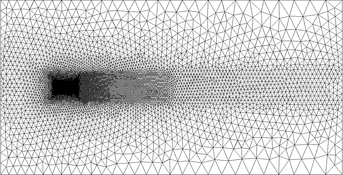
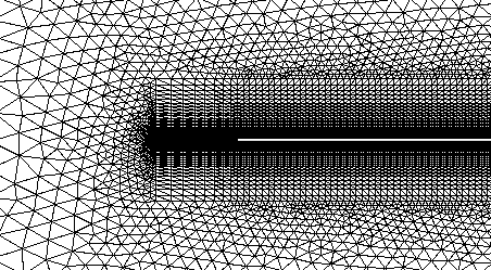
Figure 3: The initial state of the finite element mesh in the fluid domain comprising 29549 nodes and 14657 elements (left) and the close-up view of the mesh at the leading edge (right)

3.2 Validation of equivalent flexural rigidity

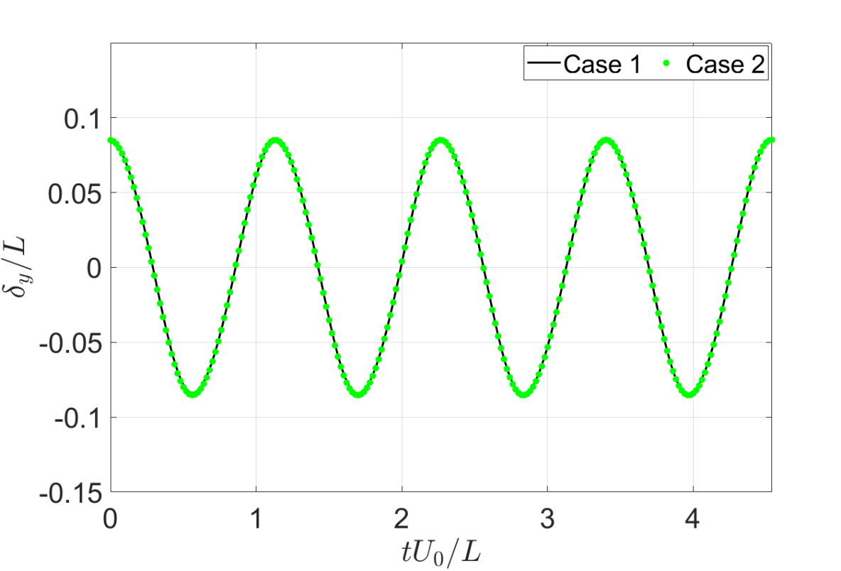
Figure 4: Tip displacement time history for cases 1 and 2, plotted against non-dimensional time.

To validate the equivalent flexural rigidity, we have compared the tip displacement time history for case 1 and case 2. The overlapping plots in Fig. 4 show that the plate tip position is the same at corresponding time instants for both cases. Therefore, the flapping amplitude and frequency response are identical for both cases. Furthermore, a substantial overlap is also observed for the time histories of the lift and drag coefficients of the plate in cases 1 and 2, as seen in Fig. 5. The force profile for the plate in both cases is analogous, resulting in similar flapping dynamics. Table 2 is a compilation of the maximum, root mean square values of tip displacement along with the mean, maximum, and root mean square values of the lift and drag coefficients. The difference between corresponding values is of the order $10^{-3}$ or less.

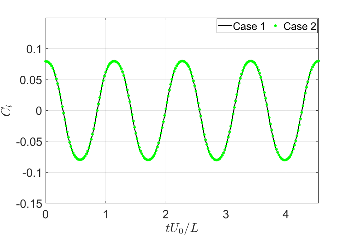
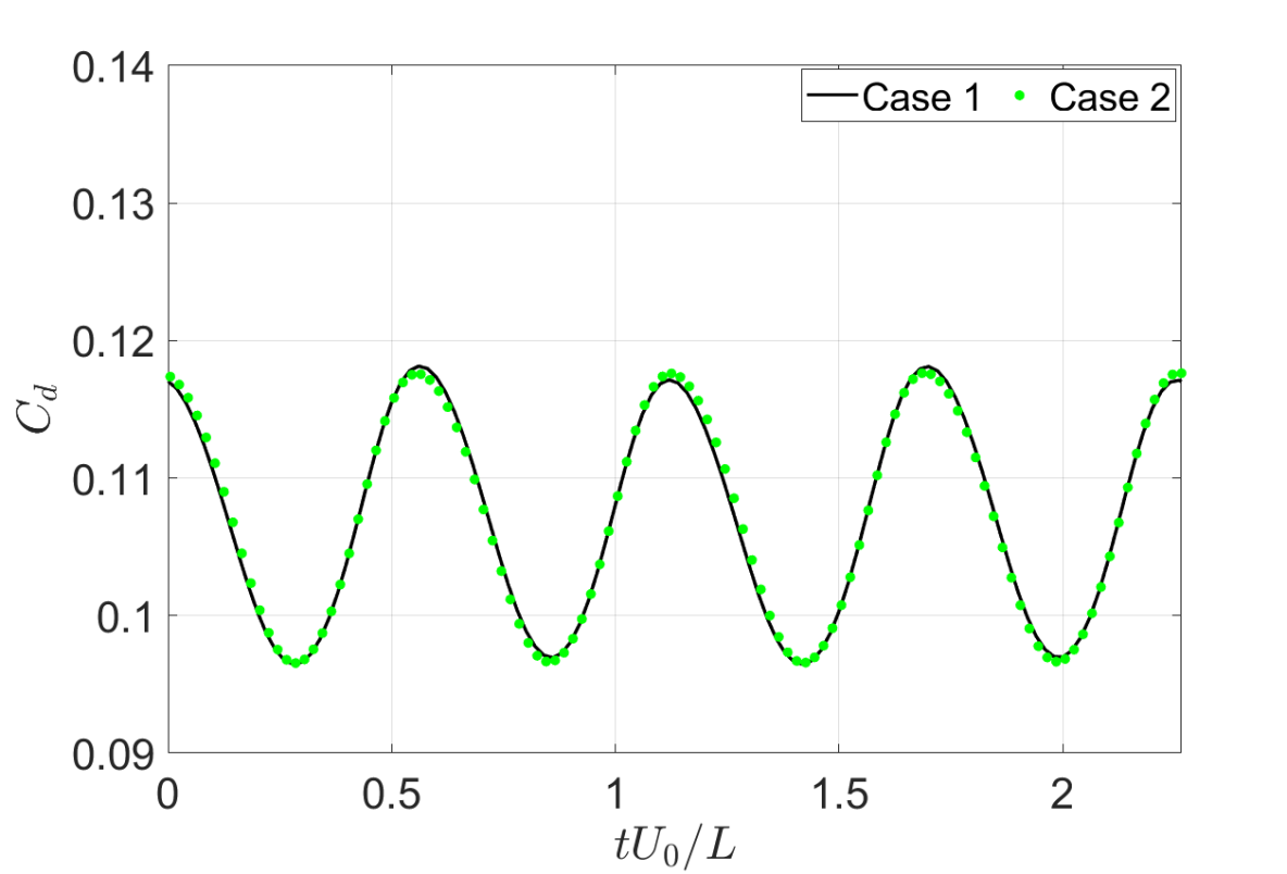
Figure 5: Temporal evolution of the co-efficient of lift (left) and co-efficient of drag (right) over four cycles corresponding to cases 1 and 2.

In addition to the similarity of the dynamic behavior of the plate, the flow around the plates also displays strong similitude for cases 1 and 2. Figure 6 shows a side-by-side comparison of the pressure, velocity and vorticity contours for both cases at the same time instant. We can observe the semblance of flow characteristics at matching time instants. Based on the similarities in both cases, we can conclude that the flapping dynamics of the plate depend on the plate’s equivalent flexural rigidity, notwithstanding the values of the flexural rigidity for the individual layers.

We have carried out the same exercise for cases 3 and 4. The flow features have been plotted at chronological, equally-spaced time instants over a half-cycle. Details of all numerical results are summarized in the supplementary material. The tip displacement and $C_{L}$, $C_{D}$ time histories for cases 4 and 5 are presented in Figs. 7 and  8 respectively. An exact overlap has also been seen in this case. Therefore, the equivalent flexural rigidity formulation holds good even for unequal layer thicknesses.

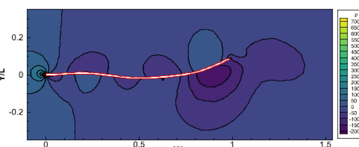
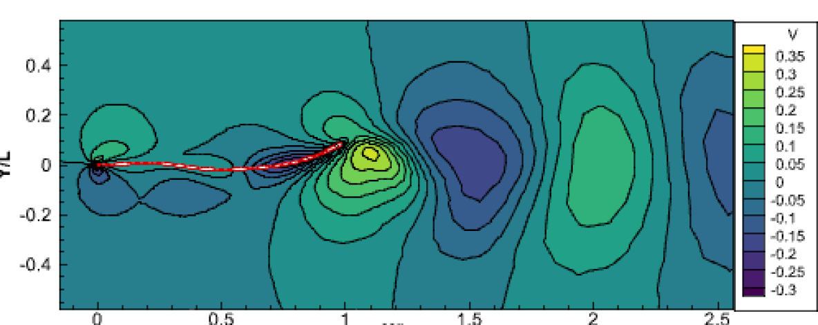
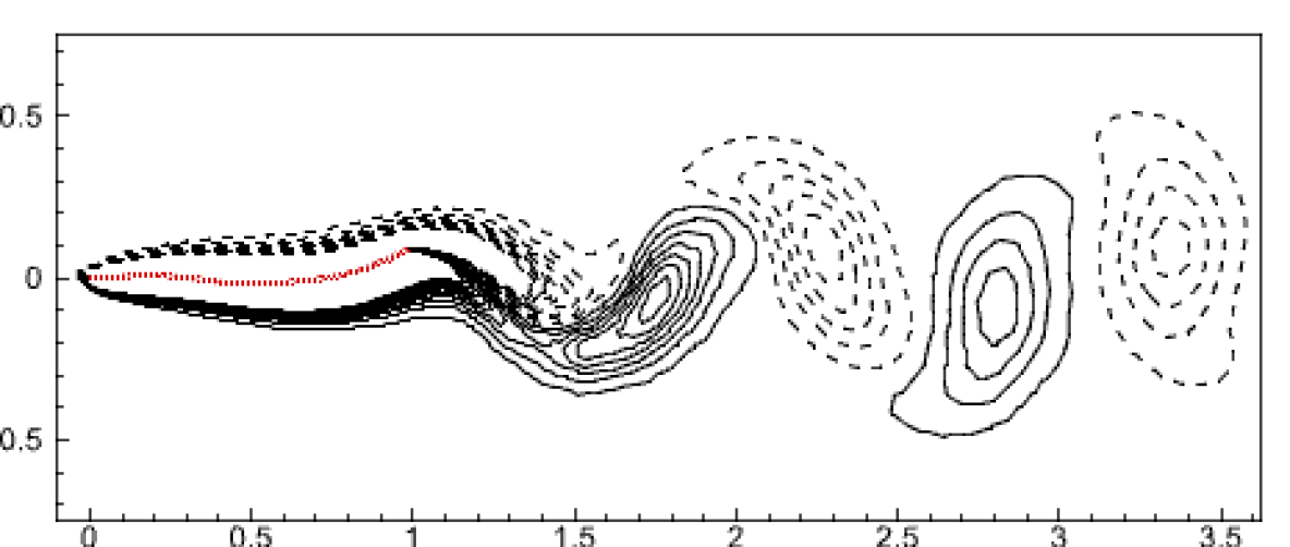
Figure 6: Pressure, velocity and vorticity contours respectively for cases 1 (left) and 2 (right).

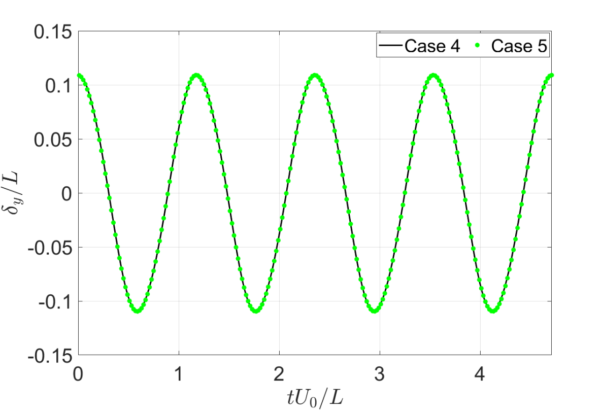
Figure 7: Tip displacement time history for cases 4 and 5, plotted against non-dimensional time.

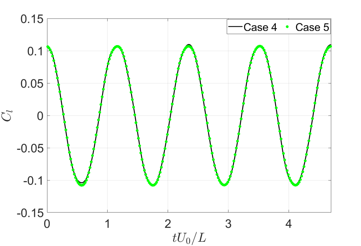
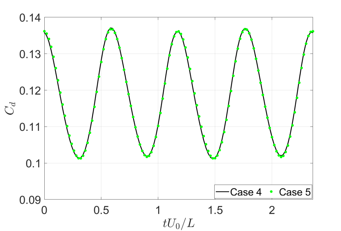
Figure 8: Temporal evolution of the co-efficient of lift (left) and co-efficient of drag (right) over four cycles corresponding to cases 4 and 5.

3.3 Validation of equivalent mass ratio

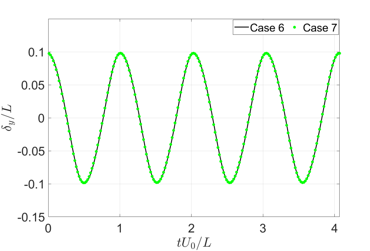
Figure 9: Tip displacement time history for cases 6 and 7, plotted against non-dimensional time.

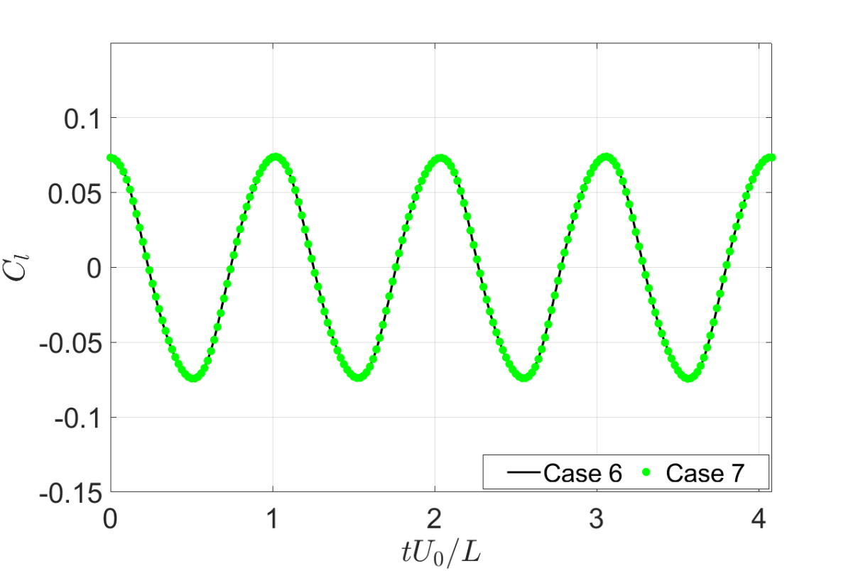
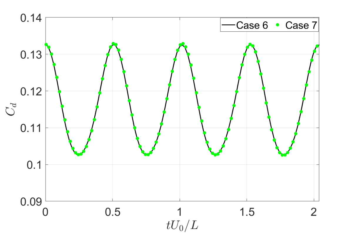
Figure 10: Temporal evolution of the co-efficient of lift (left) and co-efficient of drag (right) over four cycles corresponding to cases 6 and 7.

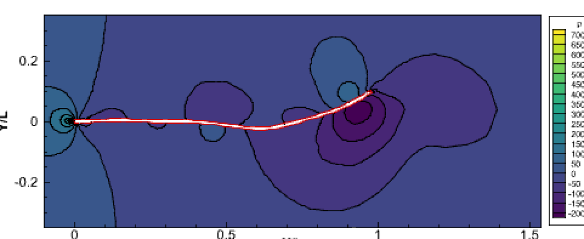
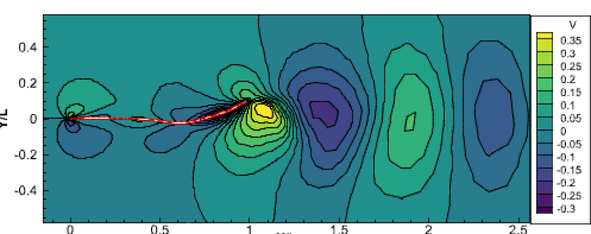
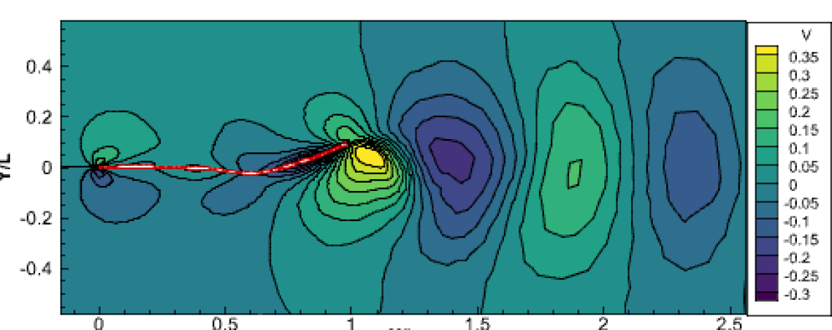
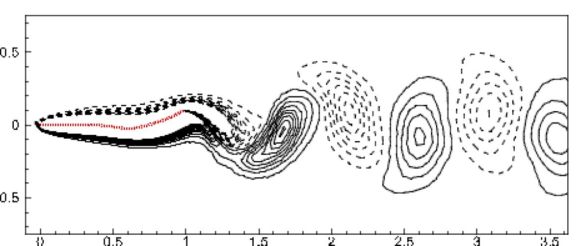
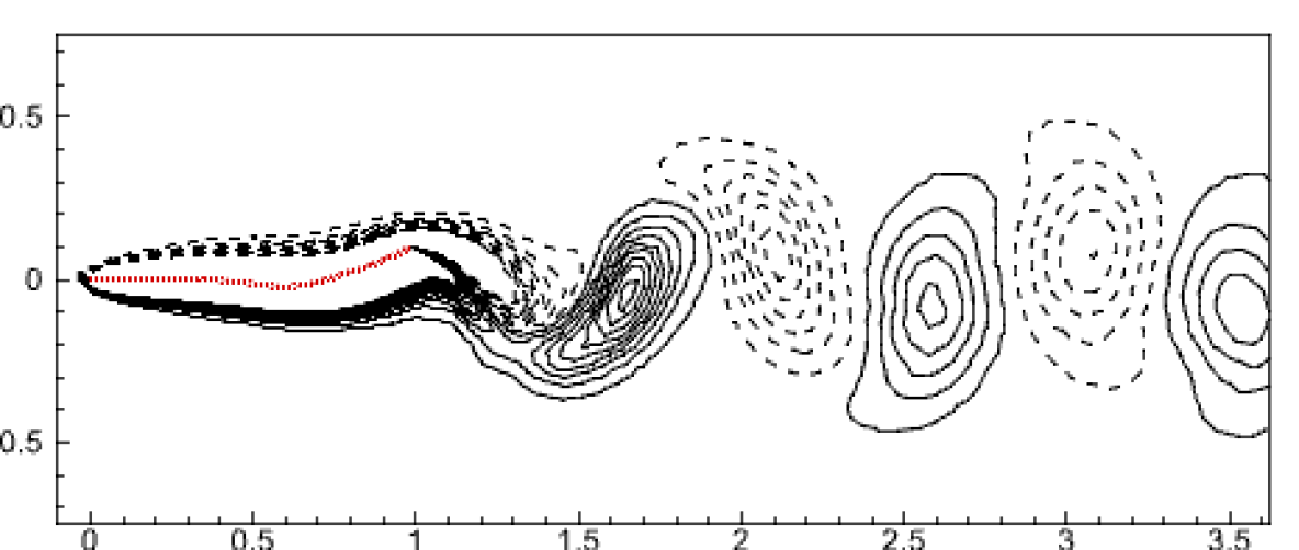
Figure 11: Pressure, velocity and vorticity contours respectively for cases 6 (left) and 7 (right).

Following the same procedure to validate the equivalent mass ratio, we present the flapping dynamics and flow characteristics for cases 6 and 7. Figure 9 shows the tip displacement time history for both cases. The plots exhibit an exact overlap leading to parity of amplitude and frequency of flapping. The agreement in the values of $C_{L}$ and $C_{D}$ of the plate in cases 6 and 7 for identical time instants is depicted in Fig. 10. A quantitative summary for these plots is available in Table 2.

The pressure, velocity and vorticity contours for cases 6 and 7 are presented in Fig. 11. Similar flow features are observed for corresponding plate configurations. Cases 8 and 9 also display similarities in the plate’s motion and the surrounding fluid’s behavior with respect to time. For case 10, we have considered an arbitrary ratio for the layer thicknesses that is not equal to 1. Figures 12 and 13 present the tip displacement, $C_{L}$ and $C_{D}$ time histories respectively, for cases 9 and 10. Here as well, an exact overlap has been observed. The sufficiently strong agreement of the results substantiates the similarity between the cases with identical non-dimensional parameters; thus, the newly proposed non-dimensional parameters effectively predict the flapping dynamics of multilayered plates.

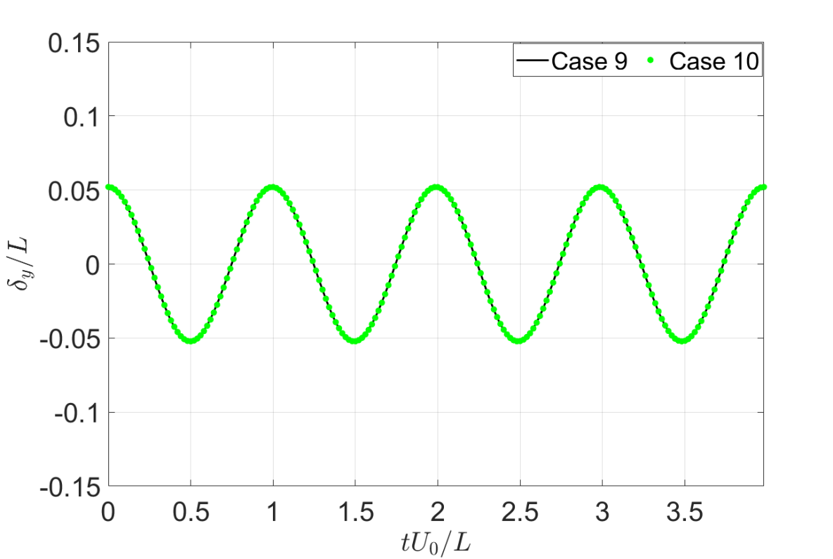
Figure 12: Tip displacement time history for cases 9 and 10, plotted against non-dimensional time.

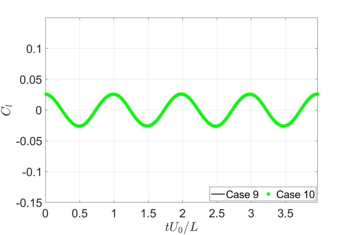
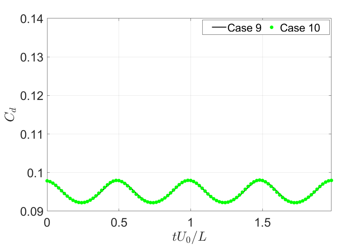
Figure 13: Temporal evolution of the co-efficient of lift (left) and co-efficient of drag (right) over four cycles corresponding to cases 9 and 10.

Table 2: Comparison of the statistical data for tip displacement, coefficient of drag and coefficient of lift of the plate obtained from numerical simulations

Case	$y_{max}$	$y_{rms}$	$C_{d}^{\mathrm{mean}}$	$C_{d}^{\mathrm{max}}$	$C_{d}^{\mathrm{rms}}$	$C_{l}^{\mathrm{max}}$	$C_{l}^{\mathrm{rms}}$
1	0.08529	0.05967	0.10709	0.11814	0.00744	0.08095	0.05890
2	0.08524	0.06008	0.10717	0.11770	0.00749	0.08019	0.05939
3	0.10943	0.07692	0.11827	0.13662	0.01234	0.10736	0.07763
4	0.10982	0.07685	0.11837	0.13734	0.01233	0.10969	0.07772
5	0.10913	0.07671	0.11822	0.13684	0.01230	0.10730	0.07757
6	0.09881	0.06864	0.11634	0.13261	0.01063	0.07376	0.05230
7	0.09821	0.06855	0.11634	0.13263	0.01062	0.07359	0.05231
8	0.05204	0.03659	0.09491	0.09803	0.00205	0.02602	0.01836
9	0.05204	0.03604	0.09490	0.09804	0.00204	0.02616	0.01838
10	0.05207	0.03645	0.09489	0.09806	0.00204	0.02611	0.01841

4 Conclusion

In this work, the definition of non-dimensional parameters that describe the flapping dynamics of an isotropic flexible plate placed in a uniform flow has been generalized for the multilayered plate. The equivalent flexural rigidity and the equivalent mass ratio are analytically derived to accommodate the shifted neutral axis. The proposed parameters are validated using numerical simulations to investigate the flapping dynamics of a two-layered plate in uniform flow. The observations prove the ability of the non-dimensional parameters to describe the cross-stream flapping and fluid flow dynamics of multilayered plates with great accuracy. Consequently, the suggested non-dimensional framework can be used to extend the existing experimental, computational, and analytical research on single-layered plates to predict the flapping dynamics of multilayered plates.

5 CRediT authorship contribution statement

Esha Jain: Validation, Formal Analysis, Investigation, Writing - Original Draft, Visualization. Aditya Karthik Saravanakumar: Software, Validation. V. Joshi: Writing - Review & Editing. P. S. Gurugubelli: Conceptualization, Methodology, Software, Supervision.

6 Declaration of Competing Interest

The authors declare that they have no known competing financial interests or personal relationships that could have appeared to influence the work reported in this paper.

7 Acknowledgments

The corresponding author would like to acknowledge the financial support from the Science and Engineering Research Board’s Start-up Research Grant (SERB-SRG) with sanction order number SRG/2019/001249 and BITS Pilani’s OPERA award.

References

- Triantafyllou et al. [2016] M. S. Triantafyllou, R. Bourguet, J. Dahl, Y. Modarres-Sadeghi, Vortex-induced vibrations. in: M. r. dhanak, n. i. xiros (eds), in: Springer Handbook of Ocean Engineering, Springer Handbooks, Springer, 2016.
- Gab [2005] An overview of modeling and experiments of vortex-induced vibration of circular cylinders, J. Sound Vib. 282 (2005) 575–616.
- Blu [2008] Influence of microcalcifications on vulnerable plaque mechanics using fsi modeling, J. Biomech. 41 (2008) 1111–1118.
- Zhang et al. [2019] L. Zhang, H. Dai, A. Abdelkefi, L. Wang, Experimental investigation of aerodynamic energy harvester with different interference cylinder cross-sections, Energy 167 (2019) 970–981.
- Meliga et al. [2011] P. Meliga, J.-M. Chomaz, F. Gallaire, Extracting energy from a flow: an asymptotic approach using vortex-induced vibrations and feedback control, J. Fluids Struct. 27 (2011) 861–874.
- Zhang et al. [2017] L. Zhang, A. Abdelkefi, H. Dai, R. Naseer, L. Wang, Design and experimental analysis of broadband energy harvesting from vortex-induced vibrations, J. Sound Vib. 408 (2017) 210–219.
- Antoine et al. [2016] G. O. Antoine, E. de Langre, S. Michelin, Optimal energy harvesting from vortex-induced vibrations of cables, Proc. R. Soc. A: Math. Phys. Eng. Sci. 472 (2016) 20160583.
- Elvin and Elvin [2011] N. G. Elvin, A. A. Elvin, An experimentally validated electromagnetic energy harvester, J. Sound Vib. 330 (2011) 2314–2324.
- Bernitsas et al. [2009] M. M. Bernitsas, Y. Ben-Simon, K. Raghavan, E. Garcia, The vivace converter: model tests at high damping and reynolds number around 105, J. Offshore Mech. Arct. Eng. 131 (2009).
- Soti et al. [2017] A. K. Soti, M. C. Thompson, J. Sheridan, R. Bhardwaj, Harnessing electrical power from vortex-induced vibration of a circular cylinder, Journal of Fluids and Structures 70 (2017) 360–373.
- Soti et al. [2018] A. K. Soti, J. Zhao, M. C. Thompson, J. Sheridan, R. Bhardwaj, Damping effects on vortex-induced vibration of a circular cylinder and implications for power extraction, Journal of Fluids and Structures 81 (2018) 289–308.
- Zhang et al. [2000] J. Zhang, S. Childress, A. Libchaber, M. Shelley, Flexible filaments in a flowings soap film as a model for one-dimensional flags in a two-dimensional wind, Nature 408 (2000) 835–839.
- Quinn et al. [2014a] D. B. Quinn, G. V. Lauder, A. J. Smits, Scaling the propulsive performance of heaving flexible panels, J. Fluid Mech. 738 (2014a) 250–267.
- Quinn et al. [2014b] D. B. Quinn, G. V. Lauder, A. J. Smits, Flexible propulsors in ground effect, Bioinspir. Biomim. 9 (2014b).
- Tang and Lu [2015] C. Tang, X. Lu, Propulsive performance of two-and three-dimensional flapping flexible plates, Theor. App. Mech. Lett. 5 (2015) 9–12.
- Hua et al. [2013] R.-N. Hua, L. Zhu, X.-Y. Lu, Locomotion of a flapping flexible plate, Phys. Fluids 25 (2013).
- Joshi and Mysa [2021] V. Joshi, R. C. Mysa, Mechanism of wake-induced flow dynamics in tandem flapping foils: Effect of the chord and gap ratios on propulsion, Phys. Fluids 33 (2021) 087104.
- Allen and Smits [2001] J. J. Allen, A. Smits, Energy harvesting eel, J. Fluids Struct. 15 (2001) 1–12.
- Tang and Paidoussis [2009] L. Tang, M. P. Paidoussis, The coupled dynamics of two cantilevered flexible plates in axial flow, J. Sound Vib. 323 (2009) 790–801.
- Akcabay and Young [2012] D. T. Akcabay, Y. L. Young, Hydroelastic response and energy harvesting potential of a flexible piezoelectric beams in viscous flow, Phys. Fluids 24 (2012) 054106.
- Kinsey and Dumas [2006] T. Kinsey, G. Dumas, Parametric study of an oscillating airfoil in power extraction regime, 24th AIAA Applied Aerodynamics Conference (2006).
- Kinsey and Dumas [2012] T. Kinsey, G. Dumas, Optimal tandem configuration for oscillating-foils hydrokinetic turbine, J. Fluids Eng.-T ASME 134 (2012).
- JEO [2005] MEMS power generator with transverse mode thin film PZT, Sens. Actuator A Phys. 122 (2005) 16 – 22. SSSAMW 04.
- Taylor et al. [2001] G. W. Taylor, J. R. Burns, S. M. Kammann, W. B. Powers, T. R. Welsh, The energy harvesting eel: A small subsurface ocean/river power generator, IEEE J. Ocean. Eng. 26 (2001) 539–547.
- Li et al. [2011] S. Li, J. Yuan, H. Lipson, Ambiemeasurements harvesting using cross-flow fluttering, J. Appl. Phys. 109 (2011).
- Akaydin et al. [2010] H. D. Akaydin, N. Elvin, Y. Andreopoulos, Wake of a cylinder: A paradigm for energy harvesting with piezoelectric materials, Exp. Fluids 49 (2010) 291.
- Kim et al. [2013] D. Kim, J. Cossé, C. Huertas Cerdeira, M. Gharib, Flapping dynamics of an inverted flag, J. Fluid Mech. 736 (2013) R1.
- Gurugubelli and Jaiman [2015] P. S. Gurugubelli, R. Jaiman, Self-induced flapping dynamics of a flexible inverted foil in a uniform flow, J. Fluid Mech. 781 (2015) 657–694.
- Orrego et al. [2017] S. Orrego, K. Shoele, A. Ruas, K. Doran, B. Caggiano, R. Mittal, S. Kang, Harvesting ambient wind energy with an inverted piezoelectric flag, App. Energy 194 (2017) 212–222.
- Shoele and Mittal [2016] K. Shoele, R. Mittal, Energy harvesting by flow-induced flutter in a simple model of an inverted piezoelectric flag, J. Fluid Mech. 790 (2016) 582–606.
- Piñeirua et al. [2015] M. Piñeirua, O. Doaré, S. Michelin, Influence and optimization of the electrodes position in a piezoelectric energy harvesting flag, J. Sound Vib. 346 (2015) 200–215.
- Peskin [2002] C. Peskin, The immersed boundary method, Acta Numer. 11 (2002) 479–517.
- Connell and Yue [2007] B. S. H. Connell, D. K. P. Yue, Flapping dynamics of a flag in a uniform stream, J. Fluid Mech. 581 (2007) 33–67.
- Tang et al. [2015] C. Tang, N.-S. Liu, X.-Y. Lu, Dynamics of an inverted flexible plate in a uniform flow, Phys. Fluids 27 (2015).
- Tian et al. [2011] F. B. Tian, H. Luo, L. Zhu, J. C. Liao, X.-Y. Lu, An efficient immersed boundary-lattice boltzmann method for the hydrodynamic interaction of elastic filaments, J. Comput. Phys. 230 (2011) 7266–7283.
- Favier et al. [2015] J. Favier, A. Revell, A. Pinelli, Numerical study of flapping filaments in a uniform fluid flow, J. Fluids Struct. 53 (2015) 26–35.
- Saravanakumar et al. [2021] A. K. Saravanakumar, K. Supradeepan, P. Gurugubelli, A numerical study on flapping dynamics of a flexible two-layered plate in a uniform flow, Phys. Fluids 33 (2021) 017108.
- Shelley et al. [2005] M. Shelley, N. Vandenberghe, J. Zhang, Heavy flags undergo spontaneous oscillations in flowing water, Phys. Rev. Lett. 94 (2005).
- Jaiman. et al. [2013] R. K. Jaiman., M. K. Parmar, P. S. Gurugubelli, Added mass and aeroelastic stability of a flexible plate interacting with mean flow in a confined channel, J. Appl. Mech. 81 (2013).