Searching for lepton portal dark matter with colliders and gravitational waves

Abstract

We study the lepton portal dark matter (DM) model in which the relic abundance is determined by the portal coupling among the Majorana fermion DM candidate $\chi$, the singlet charged scalar mediator $S^{\pm}$ and the Standard Model (SM) right-handed lepton. The direct and indirect searches are not sensitive to this model. This article studies the lepton portal coupling as well as the scalar portal coupling (between $S^{\pm}$ and SM Higgs boson), as the latter is generally allowed in the Lagrangian. The inclusion of scalar portal coupling not only significantly enhances the LHC reach via the $gg\to h^{*}\to S^{+}S^{-}$ process, but also provides a few novel signal channels, such as the exotic decays and coupling deviations of the Higgs boson, offering new opportunities to probe the model. In addition, we also study the Drell-Yan production of $S^{+}S^{-}$ at future lepton colliders, and find out that the scenario where one $S^{\pm}$ is off-shell can be used to measure the lepton portal coupling directly. In particular, we are interested in the possibility that the scalar potential triggers a first-order phase transition and hence provides the stochastic gravitational wave (GW) signals. In this case, the terrestrial collider experiments and space-based GW detectors serve as complementary approaches to probe the model.

1 Introduction

The Standard Model (SM) of particle physics has been a great triumph in explaining and predicting the astrophysical and terrestrial experimental phenomena, however there are still many unsolved problems remaining, such as the dark matter (DM). Many astrophysical evidences support the existence of DM, and the fitting result of Cosmic Microwave Background (CMB) to the $\Lambda$CDM model yields a DM relic abundance of $\Omega_{\rm DM}h^{2}\approx 0.12$ Aghanim:2018eyx , which accounts for $\sim 27\%$ of the total universe energy. However, we still know very little about the particle origin of DM, except that none of the SM particles can be the DM candidate Bertone:2004pz . Therefore, the existence of DM is a clear evidence for physics beyond the SM (BSM).

Over the past several decades, the most popular particle explanation for DM has been the freeze-out mechanism of the weakly interacting massive particles (WIMPs) Lee:1977ua , as it naturally yields the observed DM relic density when the coupling of DM to the SM particles is of the order of the electroweak (EW) gauge couplings, and the DM mass is $\mathcal{O}(100~{}{\rm GeV})$. Although the results from direct detection Schumann:2019eaa , indirect detection Gaskins:2016cha and collider searches Boveia:2018yeb have been pushing more and more stringent bounds on WIMPs, there is still room for this scenario. There are many simplified models Alves:2011wf ; Abdallah:2014hon ; Abdallah:2015ter ; Abercrombie:2015wmb describe the interactions between DM and SM particles. One category of them couples DM to SM fermions through Yukawa interaction Boehm:2003hm , which is similar to neutralino-sfermion-fermion vertex in supersymmetric (SUSY) models. The interactions can induce $t$-channel annihilation diagrams for the DM pair. Such colored Goodman:2011jq ; Garny:2012eb ; Liu:2013gba ; An:2013xka ; DiFranzo:2013vra ; Bai:2013iqa ; Papucci:2014iwa ; deSimone:2014pda ; Abdallah:2014hon ; Garny:2014waa ; Gomez:2014lva ; Baker:2015qna and uncolored Liu:2013gba ; Bai:2014osa ; Chang:2014tea ; Agrawal:2014ufa ; Garny:2015wea mediators have been studied in literature.

The lepton portal DM model is proposed in Ref. Bai:2014osa , which assumes a portal coupling among the SM lepton and two dark sector particles $S$ (scalar) and $\chi$ (fermion), where “dark sector” means an odd $\mathbb{Z}_{2}$ symmetry is assigned to $S$ and $\chi$. Depending on the mass hierarchy, the DM candidate could be $S$ or $\chi$, while the fermion DM case can be further classified into Dirac or Majorana DM scenarios. This particular model has been further studied in Refs. Yu:2014mfa ; Altmannshofer:2014cla ; Yu:2014pra ; Garny:2015wea ; Agrawal:2015tfa ; Ibarra:2015fqa ; Cai:2015zza ; Baek:2015fma ; Chen:2015jkt ; Berlin:2015njh ; Agrawal:2015kje ; Mukherjee:2015axj ; Evans:2016zau ; Chao:2016lqd ; Borah:2017dqx ; Kowalska:2017iqv ; Duan:2017pkq ; Yuan:2017ysv ; Tang:2017lfb ; Ge:2017tkd ; Ding:2017jdr ; Baker:2018uox ; Hisano:2018bpz ; Gaviria:2018cwb ; Kavanagh:2018xeh ; Kawamura:2020qxo ; Okada:2020oxh ; Ge:2020tdh ; Boehm:2020wbt ; Okawa:2020jea ; Kowalska:2020zve ; Verma:2021koo ; Alvarado:2021fbw ; Horigome:2021qof ; Bai:2021bau ; Jueid:2020yfj ; Arcadi:2021glq ; Arcadi:2021cwg ; Calibbi:2018rzv . In this article, we consider the model with right-handed lepton portal, taking $\chi$ as Majorana DM candidate and $S$ as the charged scalar mediator, which is similar to the setup in Ref. Bai:2014osa .

This model has very small indirect search cross sections due to helicity suppression. Because the DM candidate only couples to charged leptons, its nuclear recoil cross section comes from loop diagrams. Thus, the direct search signal is also suppressed. Therefore, collider experiments are crucial in probing this model. The typical collider signal is the Drell-Yan pair production of the $S^{\pm}$ mediator, and its subsequent decay to $\chi$ and a charged lepton. In this article, we study this channel at the LHC and future $e^{+}e^{-}$ colliders, and in the latter case we include the off-shell $S$ pair production $S^{\pm}S^{\mp(*)}$, which provides a direct probe for the lepton portal coupling.

Different from previous studies, in addition to the lepton portal coupling, we also consider the Higgs portal coupling $|S|^{2}|H|^{2}$, which is in general allowed in the Lagrangian. The inclusion of this coupling leads to several novel signals, such as the gluon-gluon fusion production of $S^{+}S^{-}$ at the LHC, the Higgs exotic decay (e.g. $h\to\chi\chi$, $h\to\ell^{+}\ell^{-}\chi\chi$), the Higgs coupling (e.g. $hZZ$, $h\gamma\gamma$, $h\ell^{+}\ell^{-}$) deviations and the lepton $(g-2)$ corrections to the SM prediction. In particular, the scalar portal coupling might be able to trigger a first-order phase transition (FOPT) in the early universe, opening the window for detecting the model via the stochastic gravitational wave (GW) signals. We finally consider the interplay between the GW searches and collider searches and show their complementarity.

This paper is organized as follows. We describe the model and derive the parameter space for the WIMP DM candidate in section 2. In section 3, various terrestrial searches are investigated, including the $S^{+}S^{-}$ production, the exotic decay and coupling deviations of the Higgs boson at the LHC and future $e^{+}e^{-}$ colliders, together with lepton $(g-2)$ searches to constrain the two portal couplings in this model. The scenario that this model provides the right DM relic abundance and at the same time triggers a FOPT is considered in section 4, in which we show that detectable GW signals suggest a large Higgs portal coupling. In section 5, the interplay between GW detectors and the collider experiments are discussed. Finally, we summarize and conclude in section 6.

2 The model

The model contains two new fields: the Majorana DM candidate $\chi$, which is a gauge singlet; and the complex scalar mediator $S$, which is an $SU(2)_{L}$ singlet with hypercharge $-1$. The relevant Lagrangian reads

$$\mathcal{L}_{\chi}= ~{}\frac{1}{2}\bar{\chi}i\not{\partial}\chi-\frac{1}{2}m_{\chi}\bar{\chi}\chi+y_{\ell}\left(\bar{\chi}_{L}S^{\dagger}\ell_{R}+{\rm h.c.}\right),$$ (1)

$$\mathcal{L}_{S}= ~{}\left(D^{\mu}S\right)^{\dagger}D_{\mu}S-V(H,S),$$ (2)

$$V(H,S)= ~{}\mu_{H}^{2}|H|^{2}+\mu_{S}^{2}|S|^{2}+\lambda_{H}|H|^{4}+\lambda_{S}|S|^{4}+2\lambda_{HS}|H|^{2}|S|^{2},$$ (3)

where $H$ is the SM Higgs doublet, and $\ell=e,\mu,\tau$ is the SM charged lepton (mass eigenstate). We require $S$ couple to one generation of lepton at a time to avoid lepton flavor violation. Such a flavor alignment typically needs some specific underlying mechanism to realize, which however beyond the scope of this work. For a more generic model that simultaneously involves all three flavors, our results still apply, as long as suitable rescaling is performed. The model contains a $Z_{2}$ symmetry for $\chi$ and $S$, that both of them carry odd charges. Assuming $m_{\chi}<m_{S}$, the $\chi$ is stable and thus can be the DM candidate.

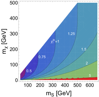
Figure 1: The lepton portal coupling $y_{\ell}^{\rm th}$ as a function of $m_{S}$ and $m_{\chi}$, which satisfies the DM relic abundance requirement.

The $\chi$ pair can annihilate into the lepton pair via the exchange of a $t$-channel $S$. Due to the Majorana nature of $\chi$, the $s$-wave component of $\chi\chi\to\ell^{+}\ell^{-}$ is suppressed by the lepton mass. Therefore, the annihilation cross section is $p$-wave dominated Garny:2013ama ; Luo:2013bua ,

$$\sigma v_{\rm rel}=\frac{y^{4}_{\ell}}{32\pi}\frac{m_{\ell}^{2}}{m_{S}^{4}}\frac{1}{(1+x)^{2}}+v_{\rm rel}^{2}\frac{y^{4}_{\ell}}{48\pi m_{S}^{2}}\frac{x(1+x^{2})}{(1+x)^{4}}\approx v_{\rm rel}^{2}\frac{y^{4}_{\ell}}{48\pi m_{S}^{2}}\frac{x(1+x^{2})}{(1+x)^{4}},$$ (4)

where $x\equiv m_{\chi}^{2}/m_{S}^{2}$, and we have applied the limit $m_{\ell}\to 0$ in the second equality. We perform the thermal average of the annihilation cross section according to Ref. Gondolo:1990dk . Given a set of $(m_{S},m_{\chi})$, one can always tune $y_{\ell}$ to have the right annihilation cross section at freeze-out to achieve the observed DM relic abundance, and the corresponding $y_{\ell}$ is denoted as $y_{\ell}^{\rm th}$, which is plotted in Fig. 1. One can see that for EW scale $m_{\chi}$ and $m_{S}$, a Yukawa coupling $y_{\ell}\sim\mathcal{O}(1)$ can provide the correct DM relic density. For $m_{\chi}<m_{S}$, smaller $m_{\chi}$ leads to larger $y_{\ell}^{\rm th}$, because the annihilation cross section scales as $m_{\chi}^{2}/m_{S}^{4}$.

As the DM annihilation signal $\chi\chi\to\ell^{+}\ell^{-}$ is helicity or $p$-wave suppressed, it is hard to be probed by satellite experiments like Fermi-LAT Ackermann:2015zua ; Fermi-LAT:2016uux , AMS-02 Accardo:2014lma ; Aguilar:2014mma , or the CMB measurements from Planck Aghanim:2018eyx . For direct detection, the scattering between $\chi$ and nucleons arises only at one-loop level, which can be described by an effective operator. Since $\chi$ is a Majorana fermion, its dimension-five magnetic dipole operator vanishes. It leaves the dimension-six operator as the leading contribution, which can be matched to the electromagnetic anapole moment of DM. This receives additional suppression from DM velocity square, so that it is difficult to detect from the direct detection experiments Bai:2014osa . As a result, we conclude that the lepton portal DM with Majorana DM has negligible signal in indirect and direct searches, and is only subject to the constraints from the thermal relic abundance and collider searches.

3 The particle experiment searches

In this section, we discuss probing the lepton portal coupling $y_{\ell}$ and Higgs portal coupling $\lambda_{HS}$ in particle experiments. First, we consider the $S^{+}S^{-}\to\ell^{+}\chi\ell^{-}\chi$ channel at the LHC and future lepton colliders. In the latter case, the off-shell production of $S^{\pm}$ offers the opportunity to probe $y_{\ell}$ directly. Next, we study the exotic decays of the Higgs and $Z$ bosons, including the three/four-body decays $h/Z\to S^{\pm(*)}S^{\mp(*)}$ and the invisible decay $h\to\chi\chi$ at the Higgs factory CEPC and FCC-ee, which probe the combination of couplings $y_{\ell}$ and $\lambda_{HS}$. Then we turn to the correction to the Higgs couplings $h\ell^{+}\ell^{-}$, $h\gamma\gamma$ and $hZZ$. Finally, the lepton $(g-2)$ is discussed.

3.1 Pair production of $S^{\pm}$

3.1.1 $pp\to S^{+}S^{-}$ at the LHC

In the model, the lepton portal scalar $S$ carries one unit of hypercharge, therefore it can be produced in pair via the EW Drell-Yan process $q\bar{q}\to Z^{*}/\gamma^{*}\to S^{+}S^{-}$ mediated by off-shell $\gamma$ and $Z$ bosons. However, in our model due to the large scalar sector coupling $\lambda_{HS}$, one can also have the (off-shell) Higgs mediated process $pp\to h^{*}\to S^{+}S^{-}$ which can significantly modify the total cross section of $pp\to S^{+}S^{-}$. For example, with $\lambda_{HS}=1$ and $m_{S}=200$ GeV, the cross section contributed by the Higgs mediation can be $30\%$ of the total cross section. The production rates of the Drell-Yan and the gluon-gluon fusion processes are shown in Fig. 2.

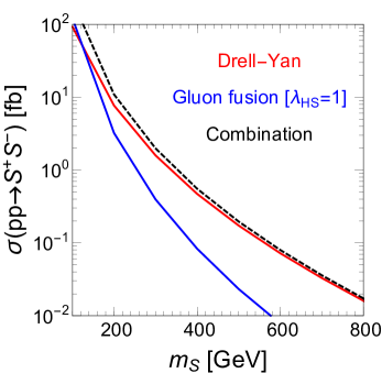
Figure 2: Left: the production rate of $S^{+}S^{-}$ at the 14 TeV LHC for the Drell-Yan (red), gluon-gluon fusion (blue) channels and their combination (black dashed). Right: the ratio of gluon-gluon fusion rate to the total cross section, for $\lambda_{HS}=1$.

The produced $S^{\pm}$ exclusively decays to $\ell^{\pm}\chi$, leading to a di-lepton plus missing transverse energy final state ($\ell^{+}\ell^{-}+\not{E}_{T}$) at the LHC. The LHC experiments have already set constraints on such a final state in searches for the sleptons from SUSY models Aad:2014vma ; Aad:2019vnb ; Aad:2019qnd . The LHC Run-I and Run-II data from ATLAS Aad:2014vma ; Aad:2019vnb have covered mass of $S^{\pm}$ up to 450 GeV for the exclusive decay channel $e^{\pm}\chi$ or $\mu^{\pm}\chi$. The compressed parameter region when $m_{\chi}$ is close to $m_{S}$, has also been studied by the ATLAS collaboration Aad:2019qnd . Earlier studies from LEP have fully excludes such charged scalar $S$ with mass $m_{S}<100$ GeV LEPslepton . We show the above existing constraints in Fig. 3 as colored regions.

To make future projections for our model, we write down the UFO model file Degrande:2011ua with the FeynRules package Alloul:2013bka and use MadGraph5_aMC@NLO Alwall:2014hca to generate parton level events, and then use Pythia8 Sjostrand:2007gs and Delphes deFavereau:2013fsa to implement parton shower and fast detector simulation, respectively. Both the EW Drell-Yan and the Higgs mediated $S^{+}S^{-}$ production processes are included in our simulation. The signal events are selected using the cuts from two signal regions (SRs) of the ATLAS study Aad:2019vnb as follows,

1. Exactly two opposite charged leptons with $p_{T}>25$ GeV and $|\eta|<2.47$;

2. At most one light-flavor jet with $p_{T}>20$ GeV and $|\eta|<2.4$, and veto the $b$-jets in such kinematic region;

3. The invariant mass $m_{\ell\ell}>100$ GeV, and transverse missing momentum $\not{E}_{T}>110$ GeV;

4. $m_{T2}>100$ or 160 GeV.

Here the $m_{T2}$ observable is defined event-by-event as the minimum of the function Lester:1999tx

$$\max\left\{m_{T}(\vec{p}_{T}^{\,\ell^{+}},\vec{p}_{T}^{\,a}),m_{T}(\vec{p}_{T}^{\,\ell^{-}},\vec{p}_{T}^{\,b})\right\},$$ (5)

subject to $\vec{p}^{\,a}+\vec{p}^{\,b}=\not{E}_{T}$, where $\vec{p}_{T}^{\,\ell^{\pm}}$ are the transverse momentum of the two charged leptons, $\vec{p}^{\,a}$ and $\vec{p}^{\,b}$ are the associated missing momenta. The transverse mass $m_{T}$ is defined as

$$m_{T}(\vec{p}_{T,1},\vec{p}_{T,2})=\sqrt{|\vec{p}_{T,1}||\vec{p}_{T,2}|(1-\cos\Delta\phi_{12})}.$$ (6)

The $m_{T2}$ cut significantly suppresses the $W^{+}W^{-}$ and $t\bar{t}$ backgrounds as their $m_{T2}$ have an end point at the $m_{W}=80.4$ GeV.

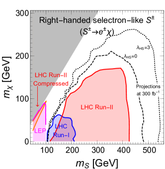
Figure 3: The current constraints for right-handed selectron-like and right-handed smuon-like scalar $S$ in the $m_{\chi}$-$m_{S}$ plane. The shaded regions are exclusions from LEP LEPslepton , LHC Run-I ($20.3~{}{\rm fb}^{-1}$) Aad:2014vma and LHC Run-II ($139~{}{\rm fb}^{-1}$) Aad:2019vnb ; Aad:2019qnd . The black lines are projections for the LHC reach at 300 ${\rm fb}^{-1}$ with $\lambda_{HS}=0$ (solid) and $\lambda_{HS}=3$ (dashed).

According to the number (1 or 2) of light-flavor jets in the final state and the different $m_{T2}$ cuts (100 or 120 GeV), we classify the events into 4 SRs, and adopt the simulated background event numbers from Ref. Aad:2019vnb . We use $S/\sqrt{B}=2$ as the criterion of the LHC reach for a given integrated luminosity, where $S$ and $B$ denote the signal and background event numbers, respectively. The projections at the 14 TeV LHC with 300 fb^-1 are plotted in Fig. 3 as black lines, where we show both the pure Drell-Yan contribution (means $\lambda_{HS}=0$, dashed) and the inclusion of gluon-gluon fusion results for $\lambda_{HS}=3$ (dotted). For large $\lambda_{HS}$, the reach can be visibly enhanced. Note that the enhancement is not significant in the low $m_{S}$ region, although in that region the gluon-gluon fusion process has a larger fraction, as shown in Fig. 2. That is because the $S^{\pm}$ from gluon-gluon fusion typically have a softer $p_{T}$, and hence they are cut away by the hard $m_{T2}$ cut in our simulation. Loosing $m_{T2}$ might help to probe the low $m_{S}$ region, and we leave the detailed study for a future work.

3.1.2 $e^{+}e^{-}\to S^{\pm}S^{\mp(*)}$ at future $e^{+}e^{-}$colliders

As shown in Fig. 3, there is a gap between the LHC and LEP constraints for $100~{}{\rm GeV}<m_{S}\lesssim 150$ GeV and $30~{}{\rm GeV}\lesssim m_{\chi}\lesssim 100$ GeV. The future $e^{+}e^{-}$ colliders with a collision energy of $\sim 250$ GeV can fill this gap. Moreover, an $e^{+}e^{-}$ machine is able to probe the lepton portal coupling $y_{\ell}$ directly, provided one $S^{\pm}$ is off-shell. For the on-shell production at LHC, since $S^{\pm}\to\ell^{\pm}\chi$ decay branching ratio is $100\%$, the rate does not depend on $y_{\ell}$. Therefore, the exclusion of slepton-like particle $S$ at LHC is shown only in the $m_{S}$-$m_{\chi}$ plot, but can not constrain $y_{\ell}$. However, for the $2\to 3$ process $e^{+}e^{-}\to S^{\pm}\ell^{\mp}\chi$ mediated by an off-shell $S^{\mp}$, the rate does depend on $y_{\ell}^{2}$, opening the window to directly probe the DM portal coupling.

The analysis is carried out on the typical Higgs factory such as CEPC, ILC or FCC-ee, with $\sqrt{s}=250$ GeV. We include the on-shell $2\to 2$ $S^{+}S^{-}$ pair production as well as the off-shell $2\to 3$ process. For $\ell=e$, the $2\to 2$ process includes both Drell-Yan contribution and the $t$-channel $\chi$ mediated contribution. Therefore, in this special case, the $2\to 2$ cross section already has the contribution of $y_{e}$. When $\ell=\mu,~{}\tau$, the cross section does not depend on $y_{\ell}$, since only Drell-Yan process contributes. Regarding $2\to 3$ process, there are two advantages to include it. One is probing the $y_{\ell}$ coupling, and the other is that we can probe $\sqrt{s}/2<m_{S}<\sqrt{s}$ region. Note that given $m_{S}$ and $m_{\chi}$, $y_{\ell}$ is determined by the relic abundance of the DM.

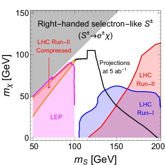
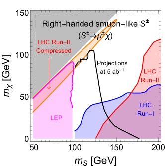
Figure 4: The current constraints for right-handed selectron-like and right-handed smuon-like scalar S in the $m_{\rm DM}$-$m_{S}$ plane. The shaded regions are exclusions from previous experiments, as stated in Fig 3. The black lines are projections for the CEPC reach at 5 ${\rm ab}^{-1}$. The zigzag shape of the projections at $m_{S}\sim 120$ GeV are due to the inclusion of off-shell contributions.

We generate signal events using the packages mentioned in section 3.1.1. Following Ref. Cao:2018ywk , we add a few cuts to select the signal events, i.e.

1. Exactly two opposite charged leptons with $p_{T}>5$ GeV and $|\eta|<3$;

2. Veto any events with a jet within $p_{T}>5$ GeV and $|\eta|<3$;

3. The transverse missing momentum $\not{E}_{T}>5$ GeV;

4. $m_{T2}>20$ GeV;

5. The polar angles of the leptons satisfy $\cos\theta_{\ell^{+}}<0.3$ and $\cos\theta_{\ell^{-}}>-0.3$.

The background event numbers are adopted from the simulated results from Ref. Cao:2018ywk . In Fig. 4, we can see that this search is complementary with the LEP and LHC results. It can cover the region $100~{}{\rm GeV}<m_{S}\lesssim 150$ GeV region, which is not touched previously when $m_{\chi}$ mass is moderately large, e.g. $30\sim 100$ GeV. For large $m_{\chi}$, the visible energy shared in the leptons decreases, which makes it hard to compete the LHC background from $W^{+}W^{-}$ pair. The cleaner environment at the lepton collider makes it sensitive to softer leptons comparing with LHC. Including $2\to 3$ process, we do see the sensitivity at future $e^{+}e^{-}$ collider extends to $m_{S}\sim 170$ GeV and $150$ GeV for $y_{e}$ and $y_{\mu}$ respectively. For small $m_{\chi}$ there is higher reach for $m_{S}$, because in this region a large $y_{\ell}$ is needed to get the correct DM abundance (see Eq. (4)), which enhances the signal significance at the collider (through the off-shell $S^{\pm}$).

3.2 Exotic decays from the Higgs and $Z$ bosons

3.2.1 Exotic decay: $h/Z\to S^{\pm(*)}S^{\mp(*)}\to\ell^{+}\chi\ell^{\prime-}\chi$

A charged $S^{\pm}$ with $m_{S}<100$ GeV is already excluded by the LEP experiment, forbidding the $h\to S^{+}S^{-}$ one-shell decay. However, for $m_{\chi}<m_{h}/2\approx 62.5$ GeV, the $\lambda_{HS}$ portal coupling can induce the exotic three- or four-body decays $h\to S^{\pm}\ell^{\mp}\chi$ or $h\to\ell^{\pm}\chi\ell^{\mp}\chi$ mediated by one or two off-shell $S^{\pm}$, depending on whether $m_{S}<m_{h}$ or not. The decay width is proportional to $y_{\ell}^{2}\lambda_{HS}^{2}$ or $y_{\ell}^{4}\lambda_{HS}^{2}$, providing a new way to probe $\lambda_{HS}$ and $y_{\ell}$. If we fix $y_{\ell}=y_{\ell}^{\rm th}$ by the relic abundance requirement, it gives a limit to $\lambda_{HS}$ for a given set of $(m_{S},m_{\chi})$.

We explore this exotic Higgs decay at the Higgs factory FCC-ee and CEPC at $\sqrt{s}=250$ GeV via the $e^{+}e^{-}\to Zh$ production channel, whose cross section is 0.24 pb. We consider the following cascade decays $Z\to\ell^{\prime\prime+}\ell^{\prime\prime-}$ and $h\to S^{\pm(*)}S^{\mp(*)}\to\ell^{+}\chi\ell^{\prime-}\chi$, where $\chi$ plays the role of missing energy. The main SM backgrounds include $ZW^{+}W^{-}$ and $Z\tau^{+}\tau^{-}$, with all the particles decaying to leptonic final states, and the $Zh$, with $h$ decaying to $W^{\pm}W^{\mp*}$, $ZZ^{*}$ and $\tau^{+}\tau^{-}$. The total cross section for the backgrounds in the $(\ell^{\prime\prime+}\ell^{\prime\prime-})\ell^{+}\ell^{\prime-}\not{E}_{T}$ final state is as small as 0.02 fb, where the leptons in the parentheses come from $Z$ decay. The signal and background events are simulated by the packages mentioned in section 3.1.1. We apply the following detailed requirements to the events,

1. At least four charged leptons with $p_{T}>10$ GeV and $|\eta|<2.47$;

2. A pair of leptons with same-flavor and opposite-sign, and satisfies $|m_{\ell^{\prime\prime+}\ell^{\prime\prime-}}-m_{Z}|<5~{}{\rm GeV}$;

3. The missing energy $\not{E}_{T}>20$ GeV;

4. The reconstructed Higgs resonance in the mass window Liu:2016zki

   $$120~{}{\rm GeV}<\sqrt{\left(p_{e^{+}}+p_{e^{-}}-p_{\ell^{\prime\prime+}}-p_{\ell^{\prime\prime-}}\right)^{2}}<130~{}{\rm GeV},$$ (7)

   which is equivalent to cut on the total energy of $Z$.

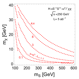
Figure 5: Left: The $95\%$ C.L. constraint on the coupling combination $\lambda_{HS}$ as contours from the exotic decay $h\to S^{\pm(*)}S^{\mp*}\to\ell^{+}\chi\ell^{\prime-}\chi$. The lepton portal coupling $y_{\ell}$ is set to be $y_{\ell}^{\rm th}$, which is the value to provide the correct DM relic abundance. Right: The $95\%$ C.L. constraint contours (magenta) for $y_{\ell}$ for the exotic decay $Z\to\ell^{+}\chi\ell^{\prime-}\chi$. The gray shaded region shows the parameter space can be excluded if $y_{\ell}=y_{\ell}^{\rm th}$.

After the cuts, for a given integrated luminosity we are able to set bounds for $\text{Br}(h\to S^{\pm(*)}S^{\mp(*)}\to\ell^{+}\chi\ell^{\prime-}\chi)$, which in turn is translated into the upper limits for $\lambda_{HS}$ once $y_{\ell}$ is fixed by the relic abundance requirement, as shown in left panel of Fig. 5. The discontinuity of the curves around $m_{S}=125$ GeV is originated from the phase space change from three-body to four-body decay. In conclusion, the future $e^{+}e^{-}$ collider can significantly constrain the couplings for light $m_{\chi}\lesssim 30$ GeV and $m_{S}$ of a few hundreds GeV.

In addition to the exotic SM Higgs decay, another good target to probe new physics is the $Z$ exotic decay Liu:2017zdh . To explore the SM parameters with better precision, the future $e^{+}e^{-}$ colliders have the proposals to run at $Z$-pole CEPCStudyGroup:2018ghi ; Abada:2019lih ; Abada:2019zxq , which can provide Giga ($10^{9}$) or Tera ($10^{12}$) $Z$ boson. Interestingly, in this model, there exists the exotic decay channel $Z\to\ell^{+}\chi\ell^{\prime-}\chi$, which provides a di-lepton plus missing energy final state. There are two types of diagrams responsible for this channel, the first one involves two off-shell $S^{\pm}$ through $ZS^{+}S^{-}$ coupling and the second one involves one off-shell $S^{\pm}$ through $Z\ell^{+}\ell^{-}$ coupling with $S$ attached to one of the charged lepton. Since we are considering $S^{\pm}$ with mass larger than 100 GeV, it is heavier than all other particles. Therefore, the decay width is dominated by the latter diagram, which is proportional to $y_{\ell}^{4}m_{S}^{-4}$.

We explore this exotic $Z$ decay similar to the Higgs case. The dominant SM background is $\bar{\nu}\nu\ell^{+}\ell^{\prime-}$ from off-shell gauge boson pair production. The cut conditions are:

1. At least two same-flavor opposite-sign leptons with $p_{T}>10$ GeV and $\eta<2.5$;

2. The missing energy should satisfy $\not{E}_{T}>10$ GeV.

The $95\%$ C.L. constraint on the exotic decay branching ratio is about $\text{Br}(Z\to e^{-}e^{+}\chi\chi)\lesssim 10^{-9}$ for Tera $Z$ option, while exact limit again depends on $m_{\chi}$ and $m_{S}$. In right panel of Fig. 5, we show the $95\%$ C.L. constraint on $y_{\ell}$ presented as the number above the magenta contours. Moreover, we compare this constraint with the thermal relic requirement $y_{\ell}^{\rm th}$. It shows that for Tera $Z$ option, the thermal DM with mass $m_{\chi}\lesssim 13$ GeV can be excluded by this exotic $Z$ search, because $y_{\ell}^{\rm th}$ exceeds the limit from the exotic $Z$ decay $Z\to e^{-}e^{+}\chi\chi$. We plot such region in gray and label as “thermal DM excluded”. This constraint provides a complimentary limit for large $m_{S}$ comparing with LHC limits, because it does not require on-shell $S$ production. Moreover, since the decay width and the DM annihilation cross section are proportional to $y_{\ell}^{4}m_{S}^{-4}$, this exclusion line can extend horizontally to very high $m_{S}$, thus is a powerful constraint for this DM model.

3.2.2 Invisible decay: $h\to\chi\chi$

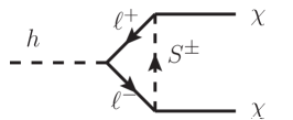
Figure 6: The one-loop induced Higgs invisible decay. The cross-diagrams for Majorana fermion $\chi$ are not shown here, but are included in the calculation.

The Higgs invisible decay $h\to\chi\chi$ is induced at one-loop level by the two Feynman diagrams listed in Fig. 6. The first diagram is negligible due to the small lepton mass. We calculate the second diagram contribution to the exotic Higgs decay using Package-X Patel:2015tea . The induced coupling is

$$\mathcal{L}_{\rm 1-loop}^{\chi}\supset\frac{1}{2}g_{h\chi\chi}h\bar{\chi}\chi,$$ (8)

where

$$g_{h\chi\chi}=-\frac{y_{\ell}^{2}\lambda_{HS}m_{\chi}v}{4\pi^{2}(4m_{\chi}^{2}-m_{h}^{2})}\times$$

$$\left[\text{DiscB}(m_{h}^{2},m_{S},m_{S})+\frac{m_{S}^{2}-m_{\chi}^{2}}{m_{\chi}^{2}}\left(\log\frac{m_{S}^{2}}{m_{S}^{2}-m_{\chi}^{2}}-m_{\chi}^{2}C_{0}(m_{h}^{2},m_{\chi}^{2},m_{\chi}^{2},m_{S},m_{S},0)\right)\right],$$

$$\approx-\frac{y_{\ell}^{2}\lambda_{HS}m_{\chi}v}{16\pi^{2}m_{S}^{2}}+\mathcal{O}\left(m_{S}^{-3}\right)$$ (9)

where DiscB is the finite part of the Passarino-Veltman function $B_{0}$ defined in Package-X, $C_{0}$ is the Passarino-Veltman function following the definition in Package-X and the lepton mass is taken to be zero. In the second equality, we have expanded the result with large $m_{S}$. We have checked our result with Ref. Djouadi:2001kba and Ref. Berlin:2015njh , and found agreement between each other. In numeric calculation, we use the full expression from Eq. (3.2.2).

The $h\to\chi\chi$ partial width is given as

$$\Gamma(h\to\chi\bar{\chi})=\frac{g_{h\chi\chi}^{2}m_{h}}{8\pi}\left(1-\frac{4m_{\chi}^{2}}{m_{h}^{2}}\right)^{\frac{3}{2}}\,.$$ (10)

The current best limit for invisible Higgs decay is $\text{Br}(h\to{\rm inv})<13\%$ at ATLAS Run-II with integrated luminosity $139~{}{\rm fb}^{-1}$ ATLAS-CONF-2020-008 . For future HL-LHC, the sensitivity for invisible Higgs BR is $3.5\%$ from Bernaciak:2014pna . For future $e^{+}e^{-}$ collider such as CEPC, the sensitivity can be increased to about $0.3\%$ CEPCStudyGroup:2018ghi .

The above projections from future colliders can set limits on the coupling combination $y_{\ell}^{2}\lambda_{HS}$ as a function of masses $m_{S}$ and $m_{\chi}$. In the left panel of Fig. 7, we show the contours of $y_{\ell}^{2}\lambda_{HS}$ for LHC (brown), HL-LHC (blue) and CEPC (red) sensitivities. The dashed and solid contours corresponds to $y_{\ell}^{2}\lambda_{HS}=1,~{}10$ respectively. We clearly see that the future $e^{+}e^{-}$ collider has a better sensitivity over the hadron colliders. In the right panel of Fig. 7, $y_{\ell}$ is set to be $y_{\ell}^{\rm th}$ to satisfy DM relic abundance requirement. Once fixing $m_{S}$ and $m_{\chi}$, the future sensitivity on $\lambda_{HS}$ can be calculated using CEPC sensitivity $\text{Br}(h\to{\rm inv})=0.3\%$ and the contours are shown. One interesting feature is that for $m_{\chi}$ smaller than 6 GeV, the sensitivity on $\lambda_{HS}$ goes down significantly, because the leading order in the width for small $m_{\chi}$ expansion is linear in $m_{\chi}$. When $m_{\chi}$ decreases further, $y_{\ell}^{\rm th}$ increases to compensate the annihilation cross section, which makes the sensitivity on $\lambda_{HS}$ becoming stronger again. Therefore, we see $\lambda_{HS}$ reaches its best sensitivity for small $m_{S}$ and moderate $m_{\chi}$.

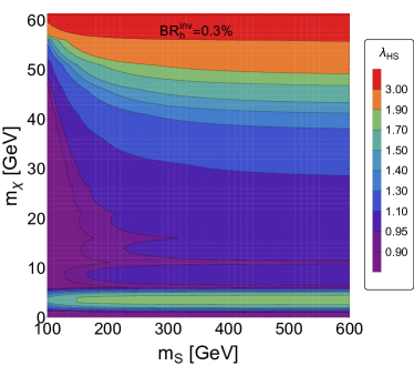
Figure 7: Left: the Higgs invisible decay as a probe for the combination $y_{\ell}^{2}\lambda_{HS}$ at different colliders. Right: the CEPC sensitivity $\text{Br}(h\to{\rm inv})<0.3\%$ can set bounds on $\lambda_{HS}$ if we fix $y_{\ell}=y_{\ell}^{\rm th}$ from the relic abundance requirement.

3.3 One-loop contributions to Higgs couplings

The $h\ell^{+}\ell^{-}$ vertex is modified by the one-loop diagram in Fig. 8, and the induced interaction is calculated using the Package-X

$$\mathcal{L}_{\rm 1-loop}^{\ell}\supset-\frac{y_{\ell}^{2}\lambda_{HS}vm_{\ell}}{8\pi^{2}m_{h}^{2}}h\bar{\ell}\ell$$ (11)

$$\times\left[1+\text{DiscB}(m_{h}^{2},m_{S},m_{S})+\frac{m_{\chi}^{2}}{m_{S}^{2}-m_{\chi}^{2}}\log\frac{m_{S}^{2}}{m_{\chi}^{2}}-\left(m_{S}^{2}-m_{\chi}^{2}\right)C_{0}(0,0,m_{h}^{2},m_{S},m_{\chi},m_{S})\right],$$

where we have taken the leading power in small lepton mass $m_{\ell}$. It is obvious that the coupling is lepton mass suppressed, because the DM only couples to right-handed lepton and one has to flip the helicity of lepton, which induce this suppression. Of course, the SM Higgs couplings to leptons are suppressed by the mass as well. Thus, the one-loop correction to the SM coupling in fraction is proportional to $y_{\ell}^{2}\lambda_{HS}/(8\pi^{2})$. In addition to vertex correction, the Higgs field renormalization and the lepton field renormalization can also contribute to the coupling. The experiments characterize the sensitivity of Higgs coupling measurements in the $\kappa$-framework Cepeda:2019klc , which is calculated using the cross section $\sigma(Zh)$ and $H$ decay branching ratios and hence the universal Higgs field renormalization effect cancels out in the decay branching ratios. Therefore, Higgs field renormalization does not affect the branching ratio to leptons. For the lepton field renormalization, it only contributes to right-handed lepton. We calculated that it is about $y_{\ell}^{2}/(128\pi^{2})$ for large $m_{S}$ expansion, which is much smaller than Eq. (11). Together with the fact that $\lambda_{HS}\gtrsim 1$, we can neglect the right-handed lepton field renormalization effect and focus on the vertex correction.

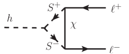
Figure 8: The one-loop induced $h\ell^{+}\ell^{-}$ coupling modification.

The most recent constraints from LHC for Higgs decay to leptons are $\text{Br}(h\to\mu^{+}\mu^{-})<3.8\times 10^{-4}$ ATLAS-CONF-2019-028 and coupling ratio $\kappa_{\tau}=1.05^{+0.16}_{-0.15}$ Aad:2019mbh . Moreover, we can also consider the sensitivities at future $e^{+}e^{-}$ collider. For example, the relative precision for coupling measurement from CEPC study in 10-parameter fit are $\delta\kappa_{\mu}<8.7\%$ and $\delta\kappa_{\tau}<1.5\%$ An:2018dwb , similar to FCC-ee study Abada:2019zxq . Therefore, we convert the above existing constraints and future sensitivities on leptons into the combination of couplings $y_{\ell}^{2}\lambda_{HS}$.

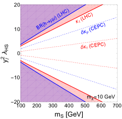
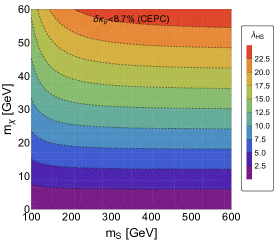
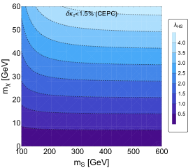
Figure 9: Left panel: The constraints on $\lambda_{HS}y_{\ell}^{2}$ from the $h\to\ell\ell$ branching ratio and coupling strength $\kappa_{\tau}$ from existing LHC constraints ATLAS-CONF-2019-028 ; Aad:2019mbh with fixed DM mass $m_{\chi}=10$ GeV. Middle and right panels: the constraint on $\lambda_{HS}$ from the projected precision $\delta\kappa_{\mu}<8.7\%$ and $\delta\kappa_{\tau}<1.5\%$ from CEPC An:2018dwb , with $y_{\ell}=y_{\ell}^{\rm th}$ by DM relic abundance.

The results are shown in Fig. 9. In the left panel, we show the limits for the combination $y_{\ell}^{2}\lambda_{HS}$ from $\text{Br}(h\to\mu^{+}\mu^{-},\tau^{+}\tau^{-}$) at LHC and CEPC. The shaded regions are already excluded by current LHC limits, while the future sensitivities from CEPC are plotted as dotted lines. The DM mass is fixed as $m_{\chi}=10$ GeV and the limits get weakened linearly with increasing $m_{S}$. In the middel and right panels, we fix $y_{\ell}=y_{\ell}^{\rm th}$ for the DM relic abundance requirement, and show the sensitivity contours for $\lambda_{HS}$ as a function of $m_{S}$ and $m_{\chi}$. When taking $m_{S}\to\infty$, the coupling in Eq. (11) is proportional to $y_{\ell}^{2}m_{S}^{-2}$. Therefore, it has the similar dependence as the DM relic abundance requirement which is $y_{\ell}^{4}m_{S}^{-4}$. This feature is clearly shown that when $m_{S}$ increases, the contours for $\lambda_{HS}$ are flat. It means that the sensitivity does not suffer for large $m_{S}$, because the large mass $m_{S}$ is compensated by large $y_{\ell}^{\rm th}$. Since for $\mu$ and $\tau$, this change of coupling ratio $\delta\kappa$ does not depend on lepton mass, the constraint on $\lambda_{HS}$ is only linear depends on the CEPC precision, which has better $\tau$ sensitivity. Therefore, the sensitivity for $\tau$ lepton portal is better by a factor of $5.8$ compared to $\mu$ lepton portal.

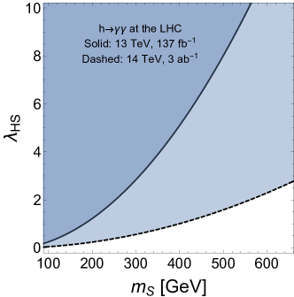
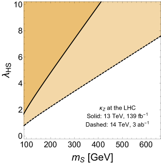
Figure 10: The shaded regions are constraints and projections from the $h\gamma\gamma$ and $hZZ$ coupling measurements at the LHC.

Besides the one-loop modification to $h\ell^{+}\ell^{-}$ coupling, the charged scalar loop can also modify the $h\gamma\gamma$ and the $hZZ$ couplings Huang:2016cjm . The former one modifies $\text{Br}(h\to\gamma\gamma)$ via the charged scalar triangle loop, and current fitting result for the signal strength is $1.12\pm 0.09$ at the 13 TeV LHC with 137 fb^-1 1851456 , while the projection accuracy is 4% at the HL-LHC Cepeda:2019klc , better than the projected sensitivity 6.9% at the 5.6 ab^-1 CEPC CEPCStudyGroup:2018ghi . The latter one is mostly contributed by Higgs field renormalization (via the $S^{\pm}$ loop) if $\lambda_{HS}>e$ (the elementary charge). This modification doesn’t rely only on $y_{\ell}$, therefore it provides a direct constraint on the scalar interaction coupling $\lambda_{HS}$ independent of the Yukawa coupling. Current constraint for $\delta\kappa_{Z}$ is 8% for the 13 TeV 139 fb^-1 LHC Aad:2020mkp , and the projected result is 1.7% at the HL-LHC Cepeda:2019klc . Therefore, the precision measurement on $Zh$ production cross section can provide a limits on $\lambda_{HS}$. Following the procedure of Ref. Huang:2016cjm , we calculate the sensitivity for $\lambda_{HS}$ from the future limits on $\text{Br}(h\to\gamma\gamma$) and the coupling strength to $Z$ gauge boson $\kappa_{Z}$. The results are presented in Fig. 10.

3.4 The lepton $g-2$

Another consequence of the lepton portal coupling $y_{\ell}$ is the magnetic dipole moment for leptons at one-loop level. The $g-2$ contribution for lepton is given as Moroi:1995yh ; Carena:1996qa

$$\Delta a_{\ell}\equiv a_{\ell}^{\rm exp}-a_{\ell}^{\rm SM}=-\frac{y_{\ell}^{2}}{16\pi^{2}}\frac{m_{\ell}^{2}}{m_{S}^{2}}\frac{1-6x+3x^{2}+2x^{3}-6x^{2}\log x}{6(1-x)^{4}},$$ (12)

where $x\equiv m_{\chi}^{2}/m_{S}^{2}$ and we keep the leading order result in the limit of small $m_{\ell}$. The last term containing $x$ in Eq. (12) is a monotonically decreasing function of $x$ and it equals to $1/6$ and $1/12$ in the limit of $x\to 0$ and $x\to 1$. Moreover, $\Delta a_{\ell}$ is always negative. The electron magnetic dipole moment has been directly measured in Refs. Hanneke:2008tm ; Hanneke:2010au , and one can compare it with the SM prediction Aoyama:2014sxa ; Mohr:2015ccw once the fine structure constant is given. The recent results are

$$\Delta a_{e}=(-88\pm 36)\times 10^{-14},\quad\Delta\tilde{a}_{e}=(48\pm 30)\times 10^{-14},$$ (13)

where $\Delta a_{e}$ comes from the $\alpha$ measurement in recent cesium recoil experiments Parker:2018vye , while $\Delta\tilde{a}_{e}$ comes from a new independent measurement using rubidium atom Morel:2020dww . For electron $g-2$, the uncertainties from QED, EW and hadronic contributions are much smaller than $\alpha$, while for muon $g-2$, the uncertainty in $\alpha$ is less significant. $\Delta a_{e}$ has a mild anomaly at confidence level of $2.4~{}\sigma$, which might need a negative contribution from new physics. However, $\Delta\tilde{a}_{e}$ turns to be positive and the significance goes down to $1.6~{}\sigma$. The measurement Morel:2020dww placed $95\%$ C.L. bounds to be $\Delta\tilde{a}_{e}\in[-34\times 10^{-14},98\times 10^{-14}]$ and we will adopt this value in the later calculation.

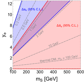
Figure 11: The interplay between $(g-2)_{e}$ and thermal DM requirements. In blue (red) shaded region, we show the range for $y_{e}$ which satisfies $\Delta a_{e}$ ($\Delta\tilde{a}_{e}$) at $95\%$ C.L with $m_{\chi}\ll m_{S}$. The gray dotdashed lines shows the thermal $y_{e}^{\rm th}$ values with different $m_{\chi}$. For both $\Delta a_{e}$ and $\Delta\tilde{a}_{e}$, $m_{\chi}$ between 1 GeV and 2 GeV can simultaneously explain $(g-2)_{e}$ and DM relic abundance.

In our model, the contribution is always negative for the electron $g-2$. In Fig. 11, We consider the $y_{e}$ range which can fit to $\Delta a_{e}$ (blue shaded region) and $\Delta\tilde{a}_{e}$ (red shaded region) at $95\%$ C.L., with a fixed $m_{\chi}$ which is much smaller than $m_{S}$. We fix $m_{\chi}=1$ GeV for $(g-2)_{e}$ fit, which satisfies the condition $m_{\chi}\ll m_{S}$ easily. For $g-2$ contribution in this limit, one can have the following expansion with small $x$ as

$$\Delta a_{\ell}\approx-\frac{y_{\ell}^{2}}{16\pi^{2}}\frac{m_{\ell}^{2}}{m_{S}^{2}}\left(\frac{1}{6}-\frac{x}{3}+\mathcal{O}(x^{2})\right).$$ (14)

Therefore, for $m_{\chi}$ considered in Fig. 11, we see that $\Delta a_{\ell}$ is determined by $m_{S}$ and $y_{\ell}$ most of the time. As a result, the blue and red shaded regions will not shift when changing to other $m_{\chi}$. On the other hand, we plot $y_{e}^{\rm th}$ with a given DM mass, which can provide the correct DM relic abundance in Fig. 11. They are plotted as dot-dashed gray lines with a fixed $m_{\chi}$. We can see that for $\Delta a_{e}$, DM mass between $0.2\sim 2$ GeV is preferred and can satisfy DM relic abundance at the same time, while for $\Delta\tilde{a}_{e}$, DM mass larger than 1 GeV is required. The two measurements have a mutual region when DM mass is between 1 and 2 GeV.

The muon $g-2$ also has a long-standing discrepancy Blum:2018mom ; Bennett:2006fi . Combination of the newest Fermilab and previous BNL measurements yields Abi:2021gix

$$\Delta a_{\mu}=(2.51\pm 0.59)\times 10^{-9},$$ (15)

corresponding to a significance of $4.2\sigma$, suggesting a positive contribution from the new physics. Unfortunately, in this lepton portal model the contribution has a negative sign that it can not explain the anomaly. To incorporate the $\Delta a_{\mu}$ result, one has to add new ingredients beyond current model.

4 Probing the model with gravitational waves

In this section we investigate the possibility of probing the scalar sector via the GWs from a FOPT in the early universe. The first subsection is devoted to the discussion of FOPT, while the second subsection studies the GW detection limits.

4.1 First-order phase transition

The scalar potential in Eq. (1) is

$$V(H,S)=\mu_{H}^{2}|H|^{2}+\mu_{S}^{2}|S|^{2}+\lambda_{H}|H|^{4}+\lambda_{S}|S|^{4}+2\lambda_{HS}|H|^{2}|S|^{2},$$

where

$$H=\frac{1}{\sqrt{2}}\begin{pmatrix}\sqrt{2}G^{+}\\ h+iG^{0}\end{pmatrix},\quad S=\frac{\phi+i\eta}{\sqrt{2}}.$$ (16)

In terms of the real components, we get

$$V(h,\phi)=\frac{\mu_{H}^{2}}{2}h^{2}+\frac{\mu_{S}^{2}}{2}\phi^{2}+\frac{\lambda_{H}}{4}h^{4}+\frac{\lambda_{S}}{4}\phi^{4}+\frac{\lambda_{HS}}{2}h^{2}\phi^{2}.$$ (17)

Here the quartic coefficients should satisfy

$$\lambda_{H}>0,\quad\lambda_{S}>0,\quad\sqrt{\lambda_{H}\lambda_{S}}+\lambda_{HS}>0,$$ (18)

to ensure the potential is bounded below.

Since $S$ has electric charge number $-1$, it cannot develop a vacuum expectation value (VEV) at zero temperature. Hence the vacuum configuration at zero temperature is along the Higgs direction, i.e. $(\left\langle h\right\rangle,\left\langle\phi\right\rangle)=(v,0)$. This means that the Higgs-relevant coefficients have been fixed by the collider measurements,

$$\mu_{H}^{2}=-\frac{m_{h}^{2}}{2},\quad\lambda_{H}=\frac{m_{h}^{2}}{2v^{2}},$$ (19)

where $m_{h}=125$ GeV and $v=246$ GeV, leaving only three free parameters in the scalar potential. If $\mu_{S}^{2}$ is positive, then the vacuum configuration $(v,0)$ is trivially achieved, because along the $\phi$ direction there is no local minimum. However, if $\mu_{S}^{2}<0$, then the $\phi$ direction also has a local minimum $w=\sqrt{-\mu_{S}^{2}/\lambda_{S}}$. In this case, to make sure $(v,0)$ is a minimum but not a saddle point, the coefficients must satisfy

$$\lambda_{H}\mu_{S}^{2}>\lambda_{HS}\mu_{H}^{2},$$ (20)

according to the Hessian matrix Bian:2019kmg . In case of $\lambda_{S}\mu_{H}^{2}>\lambda_{HS}\mu_{S}^{2}$, $(0,w)$ is also a local minimum, and a further condition

$$V(v,0)=-\frac{\mu_{H}^{4}}{4\lambda_{H}}<V(0,w)=-\frac{\mu_{S}^{4}}{4\lambda_{S}},$$ (21)

is required to ensure $(v,0)$ is the global minimum. The mass of $S$ is given by $m_{S}^{2}=\mu_{S}^{2}+\lambda_{HS}v^{2}$. Although the collider experiments have set a bound for $m_{S}$ (which also depends on $m_{\chi}$), they cannot probe $\mu_{S}^{2}$ directly and neither the sign of $\mu_{S}^{2}$. If $\mu_{S}^{2}<0$, the potential might trigger a FOPT in the early universe, and this opens a new detection scenario for this kind of DM models: the FOPT GWs.

At finite temperature, the scalar potential is modified by the thermal correction. Taking the leading gauge invariant $T^{2}$ terms Dolan:1973qd ; Braaten:1989kk , the thermal potential is

$$V_{T}(h,\phi,T)\approx\frac{\mu_{H}^{2}+c_{h}T^{2}}{2}h^{2}+\frac{\mu_{S}^{2}+c_{\phi}T^{2}}{2}\phi^{2}+\frac{\lambda_{H}}{4}h^{4}+\frac{\lambda_{S}}{4}\phi^{4}+\frac{\lambda_{HS}}{2}h^{2}\phi^{2},$$ (22)

where

$$c_{h}=\frac{3g^{2}+g^{\prime 2}}{16}+\frac{y_{t}^{2}}{4}+\frac{\lambda_{H}}{2}+\frac{\lambda_{HS}}{6},\quad c_{\phi}=\frac{g^{\prime 2}}{4}+\frac{\lambda_{S}}{3}+\frac{\lambda_{HS}}{3}.$$ (23)

The necessary condition for a FOPT is the existence of a critical temperature $T_{c}$ at which the system has two energetically degenerate vacua $(v_{c},0)$ and $(0,w_{c})$. For Eq. (22), this requires Bian:2019kmg

$$\frac{c_{\phi}}{c_{h}}<\frac{\mu_{S}^{2}}{\mu_{H}^{2}}<\frac{\sqrt{\lambda_{S}}}{\sqrt{\lambda_{H}}}<\frac{\lambda_{HS}}{\lambda_{H}},$$ (24)

and the critical temperature and VEVs are respectively

$$T_{c}=\sqrt{\frac{\mu_{H}^{2}\sqrt{\lambda_{S}}-\mu_{S}^{2}\sqrt{\lambda_{H}}}{c_{\phi}\sqrt{\lambda_{H}}-c_{h}\sqrt{\lambda_{S}}}},\quad v_{c}=\sqrt{\frac{c_{h}\mu_{S}^{2}-c_{\phi}\mu_{H}^{2}}{c_{\phi}\lambda_{H}-c_{h}\sqrt{\lambda_{H}\lambda_{S}}}}.$$ (25)

Below $T_{c}$, the Higgs-direction minimum becomes the lower one and the universe starts to decay to it from the $\phi$-direction minimum. The decay rate per unit volume reads $\Gamma(T)\sim T^{4}e^{-S_{3}/T}$, where $S_{3}$ is the classical action for the $O(3)$ symmetric bounce solution Linde:1981zj . The nucleation temperature $T_{n}$ is defined by the equality of the nucleation rate per Hubble volume and the universe expansion rate, i.e. $\Gamma(T_{n})=H^{4}(T_{n})$. For a radiation-dominated universe and a FOPT happening around the EW scale, $T_{n}$ can be solved by Quiros:1999jp

$$S_{3}/T_{n}\sim 140.$$ (26)

Eq. (26) is treated as the sufficient condition for a FOPT in this article.

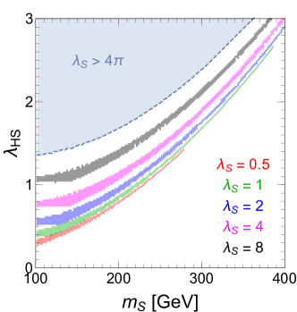
Figure 12: The parameter space allowed by a FOPT. Different colors correspond to different $\lambda_{S}$ values.

We use the Python package cosmoTransition Wainwright:2011kj to calculate the bounce solution and hence $T_{n}$ for the potential in Eq. (22). As discussed before, after taking into account the Higgs mass and VEV, in the scalar potential there are only three free parameters, which we choose to be $\lambda_{S}$, $m_{S}$ and $\lambda_{HS}$. For a fixed $\lambda_{S}$, the parameter space allowed by the FOPT can be projected to the $m_{S}$-$\lambda_{HS}$ plane. We plot the parameter space for different $\lambda_{S}$ as shaded areas in Fig. 12. The shapes of those areas can be well understood by the analytical relation Eq. (24). A sizable $\lambda_{HS}$ is preferred by FOPT, because the phase transition is triggered by the potential barrier induced by the $\lambda_{HS}h^{2}S^{2}/2$ term.

4.2 Gravitational waves

Stochastic GWs are produced during a FOPT via bubble collision Huber:2008hg ; Di:2020nny , sound waves in the plasma Hindmarsh:2015qta and the magneto-hydrodynamics turbulence Binetruy:2012ze ; Caprini:2009yp . The expanding bubble wall only accelerates for a short time before it reaches its final velocity $v_{b}<1$. Therefore, only a tiny fraction of FOPT energy deposits in the bubble shell, and the bubble collision contribution to the GWs is negligible. Instead, most of the phase transition energy is pumped into the surrounding fluid shells, making sound waves the dominant contribution to FOPT GWs Ellis:2018mja . However, the sound wave period only lasts for a finite time, after which the energy in the bulk fluid will cause the turbulence, which is another source for GWs Ellis:2020awk . Consequently, the GW spectrum today can be expressed as

$$\Omega_{\rm GW}(f)=\Omega_{\rm sw}(f)+\Omega_{\rm turb}(f),$$ (27)

where $f$ is the frequency, the subscripts “sw” and “turb” denote sound waves and turbulence respectively, and $\Omega_{\rm GW}$ is the ratio of GW energy density to the critical energy of the current universe, i.e.

$$\Omega_{\rm GW}(f)=\frac{1}{\rho_{c}}\frac{\rho_{\rm GW}}{d\ln f},$$ (28)

where $\rho_{c}=3H_{0}^{2}/(8\pi G)$, with $H_{0}$ being the Hubble constant today.

The sound wave and turbulence spectra can be expressed as functions of two FOPT parameters Grojean:2006bp ; Caprini:2015zlo ; Caprini:2019egz ,

$$\alpha=\frac{1}{g_{*}\pi^{2}T_{n}^{4}/30}\left(T\frac{\partial\Delta V_{T}}{\partial T}-\Delta V_{T}\right)\Big{|}_{T_{n}};\quad\beta/H=T_{n}\frac{d(S_{3}/T)}{dT}\Big{|}_{T_{n}},$$ (29)

where $\Delta V_{T}$ denotes the (negative) effective potential difference between the true and false vacua, and $g_{*}\sim 100$ is the number of relativistic degrees of freedom during FOPT. Namely, $\alpha$ is the ratio of FOPT latent heat to the radiation energy, while $\beta/H$ is the inverse ratio of FOPT duration to the universe expansion time scale. Numerically, the sound waves spectrum is Hindmarsh:2015qta

$$\Omega_{\rm sw}(f)h^{2}=2.65\times 10^{-6}\frac{1}{\beta/H}\left(\frac{\kappa_{v}\alpha}{1+\alpha}\right)^{2}\left(\frac{g_{*}}{100}\right)^{-1/3}v_{b}\left(\frac{f}{f_{\rm sw}}\right)^{3}\left(\frac{7}{4+3(f/f_{\rm sw})^{2}}\right)^{7/2},$$ (30)

where

$$f_{\rm sw}=1.9\times 10^{-2}~{}{\rm mHz}\times\frac{\beta/H}{v_{b}}\left(\frac{T_{n}}{100~{}{\rm GeV}}\right)\left(\frac{g_{*}}{100}\right)^{1/6}.$$ (31)

To take into account the finite duration of the sound wave period, we make the replacement $\Omega_{\rm sw}(f)\to\Omega_{\rm sw}(f)H(T_{n})\tau_{\rm sw}$ in Eq. (30) Ellis:2020awk ; Wang:2020jrd , where

$$\tau_{\rm sw}={\rm min}\left\{\frac{1}{H(T_{n})},\frac{v_{b}(8\pi)^{1/3}}{\beta\bar{U}_{f}}\right\},\quad\bar{U}_{f}=\sqrt{\frac{3}{4}\frac{\kappa_{v}\alpha}{1+\alpha}}.$$ (32)

A more accurate treatment for the sound wave cutoff factor can be found in Ref. Guo:2020grp .

The turbulence spectrum is Binetruy:2012ze ; Caprini:2009yp

$$\Omega_{\rm turb}(f)h^{2}=3.35\times 10^{-4}\frac{v_{b}}{\beta/H}\left(\frac{\kappa_{\rm turb}\alpha}{1+\alpha}\right)^{3/2}\left(\frac{g_{*}}{100}\right)^{-1/3}S_{\rm turb}(f),$$ (33)

where

$$S_{\rm turb}(f)=\frac{(f/f_{\rm turb})^{3}}{\left[1+(f/f_{\rm turb})\right]^{11/3}(1+8\pi f/h_{*})},\quad h_{*}=16.5\times 10^{-3}~{}{\rm mHz}\left(\frac{T_{n}}{100~{}{\rm GeV}}\right)\left(\frac{g_{*}}{100}\right)^{1/6},$$ (34)

and

$$f_{\rm turb}=2.7\times 10^{-2}~{}{\rm mHz}\times\frac{\beta/H}{v_{b}}\left(\frac{T_{n}}{100~{}{\rm GeV}}\right)\left(\frac{g_{*}}{100}\right)^{1/6}.$$ (35)

The factor $\kappa_{v}$ and $\kappa_{\rm turb}$ in Eq. (30) and Eq. (33) are the fraction of FOPT energy that is transformed to bulk motion/turbulence, respectively. We have adopted $\kappa_{\rm turb}=0.05\kappa_{v}$, and $\kappa_{v}$ is extracted from the numerical function of Ref. Espinosa:2010hh . $v_{b}=0.6$ is used as a benchmark in our study, although it might be calculated using the hydrodynamics.

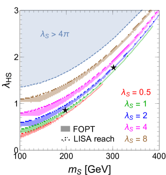
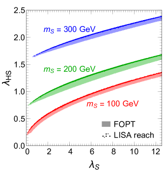
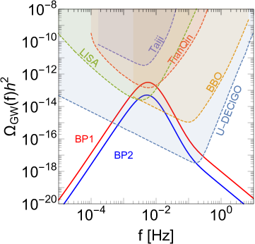
Figure 13: Top: the parameter space that triggers FOPT and can be probed by LISA, projected to different 2-dimension planes. Bottom: the GW spectrum from two benchmark points which are labeled as stars in the top left panel.

The GWs from a FOPT around EW scale might be probed by the next generation space-based laser interferometers such as LISA Audley:2017drz , BBO Crowder:2005nr , TianQin Luo:2015ght ; Hu:2017yoc , Taiji Hu:2017mde ; Guo:2018npi and DECIGO Kawamura:2011zz ; Kawamura:2006up . The detectability of GW signals can be characterized by the signal-to-noise ratio (SNR). Taking the LISA detector as an example, the SNR is defined as Caprini:2015zlo

$${\rm SNR}=\sqrt{\mathcal{T}\int_{f_{\rm min}}^{f_{\rm max}}df\left(\frac{\Omega_{\rm GW}(f)}{\Omega_{\rm LISA}(f)}\right)^{2}},$$ (36)

where $\Omega_{\rm LISA}$ is the sensitive curve of the LISA detector Caprini:2015zlo (in which we take the C1 configuration as a benchmark), and $\mathcal{T}=9.46\times 10^{7}$ s is the data-taking duration Caprini:2019egz . We adopt ${\rm SNR}=10$ as the detectable threshold, and found that for a fixed $\lambda_{S}$, only a narrow band of parameter space in Fig. 12 can be probed. The parameter space that can be probed by LISA is plotted in the top panel of Fig. 13, where we show the results both in the $m_{S}$-$\lambda_{HS}$ plane (for fixed $\lambda_{S}$) and the $\lambda_{S}$-$\lambda_{HS}$ plane (for fixed $m_{S}$). In the bottom panel of the same figure we plot the GW spectrum for two benchmark points:

$$\begin{split}{\rm BP1}:\quad&m_{S}=198~{}{\rm GeV},~{}\lambda_{HS}=0.86,~{}\lambda_{S}=1,\\ &T_{n}=76.6~{}{\rm GeV},~{}v_{n}=189~{}{\rm GeV},~{}w_{n}=94.9~{}{\rm GeV},~{}\alpha=0.0834,~{}\beta/H=228;\\ {\rm BP2}:\quad&m_{S}=302~{}{\rm GeV},~{}\lambda_{HS}=1.78,~{}\lambda_{S}=2,\\ &T_{n}=91.8~{}{\rm GeV},~{}v_{n}=123~{}{\rm GeV},~{}w_{n}=53.1~{}{\rm GeV},~{}\alpha=0.0248,~{}\beta/H=177;\\ \end{split}$$ (37)

where $(0,w_{n})$ and $(v_{n},0)$ are respectively the old and new vacua at the nucleation temperature $T_{n}$.

5 The interplay between phase transition and particle searches

In this section, we revisit the parameter space for $\lambda_{HS}$ from GW study and the corresponding constraints from the collider studies. We focus on how the two different types of experiments can be complimentary with each other. For GW experiment, we focus on the LISA detectable parameter space in the left panel of Fig. 13. Clearly, the scalar $S$ self-interaction coupling $\lambda_{S}$ can affect the LISA detectable parameter space. Therefore, we vary $\lambda_{S}$ between $0$ and $4\pi$ to obtain the entire GW detectable region for a FOPT.

5.1 Interplay with $pp\to S^{+}S^{-}$ at the LHC

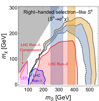
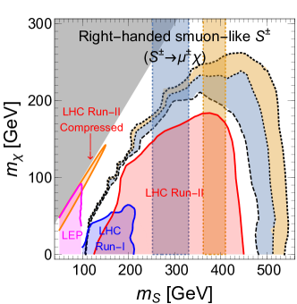
Figure 14: The interplay between gravitational wave detection and LHC searches. The collider constrains and projections are the same as those in Fig. 3. The light blue (orange) shaded region corresponds to $\lambda_{HS}=2$ (3), with the vertical boxed boundary regions being the LISA-detectable parameter space, while the irregular boundary regions being enhanced part of the LHC projections when including the $gg\to h^{*}\to S^{+}S^{-}$ contribution.

The $S^{\pm}$ particles can be pair produced at the LHC via Drell-Yan and gluon-gluon fusion processes, and the current constrains and future projections at the 14 TeV LHC has been studied in Section 3.1.1. As shown in Fig. 3, a non-zero $\lambda_{HS}$ can visibly enhance the probe limit in parameter space due to the $gg\to h^{*}\to S^{+}S^{-}$ contribution to the signal events. On the other hand, a sizable $\lambda_{HS}$ may trigger a FOPT and hence give detectable GW signals as well.

The interplay between the LHC and the future LISA experiments is plotted in Fig. 14. The light blue (orange) shaded region corresponds to $\lambda_{HS}=2$ (3), with the vertical boxed boundary regions being the LISA-detectable parameter space, while the irregular boundary regions being the enhanced LHC projections when including the $gg\to h^{*}\to S^{+}S^{-}$ contribution. This is because the GW signals is independent of the DM mass $m_{\chi}$. For a given $\lambda_{HS}$, there is a set of upper and lower bounds for $m_{S}$ in the LISA-detectable region. The enhanced parts of the LHC probe region due to $\lambda_{HS}$ are also shown in the figure. We see that the LHC and GW experiments mainly serve as complementary approaches to probe the DM parameter space; while they also have some intersections, which can be used to identify the origin of the excess (if found).

5.2 Higgs precision measurement at the future $e^{+}e^{-}$ colliders

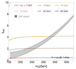
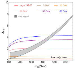
Figure 15: The interplay between gravitational wave detection and future $e^{+}e^{-}$ collider searches. The gray shaded region is the LISA detectable parameter space, varying $\lambda_{S}$ from 0 to $4\pi$. From left to right, we show the sensitivities for $\lambda_{HS}$ from future CEPC precision measurements, based on invisible Higgs decay branching ratio $\text{Br}(h\to{\rm inv})=0.3\%$, Higgs leptonic coupling precision reaches $\delta\kappa_{\mu}<8.7\%$ and $\delta\kappa_{\tau}<1.5\%$.

The collider constraints on $\lambda_{HS}$ have to be related with SM Higgs. The constraint from exotic Higgs decay is less sensitive compared to the Higgs 1-loop coupling as shown in the previous section. The 1-loop induced Higgs couplings include the coupling to $\chi\chi$ and $\ell^{+}\ell^{-}$. The former can be revealed by the Higgs invisible decay branching ratio, for example we consider the future sensitivity from CEPC $\text{Br}(h\to{\rm inv})=0.3\%$. The latter can be revealed by the Higgs precision measurements at CEPC with relative precision of couplings $\delta\kappa_{\mu}<8.7\%$ and $\delta\kappa_{\tau}<1.5\%$. In Fig. 15, we take the DM mass $m_{\chi}=1,~{}5,~{}10,~{}30,~{}50,~{}60$ GeV respectively to show its effect on the sensitivities for $\lambda_{HS}$. For a fixed DM mass, the corresponding colored line shows the maximum allowed $\lambda_{HS}$ from the future $e^{+}e^{-}$ collider searches. In general, the exclusion power is better for light DM mass $m_{\chi}$.

In the left panel of Fig. 15, one can see that for $m_{\chi}<40$ GeV the constraints on $\lambda_{HS}$ are quite similar. The reason is that the 1-loop induced coupling is proportional to $y^{2}_{\ell}\lambda_{HS}m_{\chi}/m_{S}^{2}$ for large $m_{S}$. At the same time, the annihilation cross section is proportional to $y^{4}_{\ell}m_{\chi}^{2}/m_{S}^{4}$ which requires this combination to be a constant to satisfy the relic abundance. Therefore, the limits on $\lambda_{HS}$ from Higgs invisible decay is a constant. The colored lines in the left panel do show this feature, except when $m_{S}$ is too close to the Higgs mass and the expansion on large $m_{S}$ is not valid anymore, the sensitivity on $\lambda_{HS}$ changes slightly. For larger $m_{\chi}$, the sensitivity of $\lambda_{HS}$ is downgraded because the phase space suppression in the $h\to\chi\chi$ decay. It is worth to mention that the sensitivity from Higgs invisible decay works equally good for all three flavors of lepton portals. This search can test most of the LISA detectable parameter regions for $m_{\chi}<m_{h}/2$.

In the right panel of Fig. 15, the limits from $\delta\kappa_{\tau}<1.5\%$ are plotted for different DM mass. For large $m_{S}$, we can see that the constraints on $\lambda_{HS}$ are proportional to $m_{\chi}$. The reason is that the one-loop induced Higgs coupling is roughly proportional to $y^{2}_{\ell}\lambda_{HS}m_{\ell}/m_{S}^{2}$ for large $m_{S}$ expansion. Since the relic abundance fix the combination $y^{2}_{\ell}m_{\chi}/m_{S}^{2}$ to be constant, the sensitivity for $\lambda_{HS}$ from Higgs precision measurement is proportional to $m_{\chi}$. Different from Higgs invisible branching ratio, there is no phase space suppression for $m_{\chi}\sim m_{h}/2$. One can see that for $m_{\chi}\lesssim 20$ GeV, the Higgs-tau coupling precision measurement is the most sensitive among the three panels in the figure, while for the intermediate mass $m_{\chi}$ between $20$ to $\sim 50$ GeV the Higgs invisible branching ratio measurement is better. For $m_{\chi}$ close to $m_{h}/2$, the Higgs-tau coupling measurement becomes better again due to the phase space suppression in the Higgs invisible decay.

In the middle panel of Fig. 15, we show the limits from $\delta\kappa_{\mu}<8.7\%$. The results from muon coupling measurements are fully analogous to tau coupling. The sensitivity is worse by a constant factor from $\delta\kappa_{\tau}/\delta\kappa_{\mu}$, reflecting the fact that more taus are produced due to larger Higgs-tau coupling.

Finally, it should be mentioned that the limits on $\lambda_{HS}$ from $\text{Br}(h\to\gamma\gamma)$ and $\sigma(Zh)$ are also very powerful as shown in section 3.3 and are able to exclude most of the parameter space for GW detection Huang:2016cjm . Such constraints are independent of the DM Yukawa coupling $y_{\ell}$ and therefore, are complementary with the limits from $h$ invisible and leptonic decays.

6 Conclusions

The GW detection opens a new window to the FOPT and the Higgs precision measurement is an inevitable path after the Higgs discovery. In this paper, we study their interplay in a specific DM model, namely lepton portal DM model. We emphasize the Higgs portal coupling in this model, which is neglected in the previous literature. The impact is investigated in two aspects. In the cosmological aspect, we have studied the parameter space allowing a FOPT and yielding detectable GW signals at the future detectors, taking LISA as an example. In the particle aspect, we have considered various new channels to further test this model:

• $pp\to S^{+}S^{-}$ at the LHC, which mainly probes $m_{S}$ and $m_{\chi}$ since the production is dominated by the Drell-Yan process, can also test the Higgs portal coupling between $h$ and $S^{\pm}$ (i.e. $\lambda_{HS}$) through the gluon-gluon fusion process.

• $e^{+}e^{-}\to S^{\pm}S^{\mp(*)}$ at the future lepton colliders, which can fill in the gaps between the LEP and LHC constrains ($100~{}{\rm GeV}\lesssim m_{S}\lesssim 150$ GeV), and probe the $y_{\ell}$ coupling via the off-shell production of $S^{\pm}$.

• Exotic decays of $h$ and $Z$ at the future lepton colliders, which probe the couplings $\lambda_{HS}$ and/or $y_{\ell}$ for the low $m_{\chi}$ region.

• Higgs precision measurements for invisible decay branching ratios and leptonic coupling originated from one-loop contributions, which can provide the best sensitivity for the combination $y_{\ell}^{2}\lambda_{HS}$ or $\lambda_{HS}$ assuming $y_{\ell}$ satisfies the DM relic abundance requirement.

• Electron $g-2$ experiments have recently came up with two sets of results. For $\Delta\tilde{a}_{e}$, DM mass should be larger than $1$ GeV, while for $\Delta a_{e}$, DM mass between $0.2\sim 2$ GeV is preferred.

In summary, the future Higgs precision measurements can effectively interplay with GW detection, since they both rely on the Higgs portal coupling. The Higgs portal is allowed by this model and can contribute to the Higgs couplings to DM and SM leptons at one-loop level. Therefore, most of the GW detectable parameter space can be cross-checked by the Higgs precision measurement. It shows the rigorous interplay between the future Higgs precision measurement program and the GW detection program. Specific to the lepton portal DM model, which is hard to probe through DM direct and indirect detections, the Drell-Yan production of charged scalar pair is the useful way to probe this model but only constrains the mass parameter of the scalar and DM. We studied the Higgs mediated $S^{\pm}$ pair production, exotic decays of $h/Z$ and electron $g-2$ experiment, which can help extending the constraints on mass parameters and also providing useful constraints on the Yukawa and scalar portal couplings.

References

- (1) Planck collaboration, N. Aghanim et al., “Planck 2018 results. VI. Cosmological parameters,”Astron. Astrophys. 641 (2020) A6, [1807.06209].
- (2) G. Bertone, D. Hooper and J. Silk, “Particle dark matter: Evidence, candidates and constraints,”Phys. Rept. 405 (2005) 279–390, [hep-ph/0404175].
- (3) B. W. Lee and S. Weinberg, “Cosmological Lower Bound on Heavy Neutrino Masses,”Phys. Rev. Lett. 39 (1977) 165–168.
- (4) M. Schumann, “Direct Detection of WIMP Dark Matter: Concepts and Status,”J. Phys. G 46 (2019) 103003, [1903.03026].
- (5) J. M. Gaskins, “A review of indirect searches for particle dark matter,”Contemp. Phys. 57 (2016) 496–525, [1604.00014].
- (6) A. Boveia and C. Doglioni, “Dark Matter Searches at Colliders,”Ann. Rev. Nucl. Part. Sci. 68 (2018) 429–459, [1810.12238].
- (7) LHC New Physics Working Group collaboration, D. Alves, “Simplified Models for LHC New Physics Searches,”J. Phys. G 39 (2012) 105005, [1105.2838].
- (8) J. Abdallah et al., “Simplified Models for Dark Matter and Missing Energy Searches at the LHC,” 1409.2893.
- (9) J. Abdallah et al., “Simplified Models for Dark Matter Searches at the LHC,”Phys. Dark Univ. 9-10 (2015) 8–23, [1506.03116].
- (10) D. Abercrombie et al., “Dark Matter Benchmark Models for Early LHC Run-2 Searches: Report of the ATLAS/CMS Dark Matter Forum,”Phys. Dark Univ. 27 (2020) 100371, [1507.00966].
- (11) C. Boehm and P. Fayet, “Scalar dark matter candidates,”Nucl. Phys. B683 (2004) 219–263, [hep-ph/0305261].
- (12) J. Goodman and W. Shepherd, “LHC Bounds on UV-Complete Models of Dark Matter,” 1111.2359.
- (13) M. Garny, A. Ibarra, M. Pato and S. Vogl, “Closing in on mass-degenerate dark matter scenarios with antiprotons and direct detection,”JCAP 11 (2012) 017, [1207.1431].
- (14) J. Liu, B. Shuve, N. Weiner and I. Yavin, “Looking for new charged states at the LHC: Signatures of Magnetic and Rayleigh Dark Matter,”JHEP 07 (2013) 144, [1303.4404].
- (15) H. An, L.-T. Wang and H. Zhang, “Dark matter with -channel mediator: a simple step beyond contact interaction,”Phys. Rev. D 89 (2014) 115014, [1308.0592].
- (16) A. DiFranzo, K. I. Nagao, A. Rajaraman and T. M. P. Tait, “Simplified Models for Dark Matter Interacting with Quarks,”JHEP 11 (2013) 014, [1308.2679].
- (17) Y. Bai and J. Berger, “Fermion Portal Dark Matter,”JHEP 11 (2013) 171, [1308.0612].
- (18) M. Papucci, A. Vichi and K. M. Zurek, “Monojet versus the rest of the world I: t-channel models,”JHEP 11 (2014) 024, [1402.2285].
- (19) A. De Simone, G. F. Giudice and A. Strumia, “Benchmarks for Dark Matter Searches at the LHC,”JHEP 06 (2014) 081, [1402.6287].
- (20) M. Garny, A. Ibarra, S. Rydbeck and S. Vogl, “Majorana Dark Matter with a Coloured Mediator: Collider vs Direct and Indirect Searches,”JHEP 06 (2014) 169, [1403.4634].
- (21) M. A. Gomez, C. B. Jackson and G. Shaughnessy, “Dark Matter on Top,”JCAP 12 (2014) 025, [1404.1918].
- (22) M. J. Baker et al., “The Coannihilation Codex,”JHEP 12 (2015) 120, [1510.03434].
- (23) Y. Bai and J. Berger, “Lepton Portal Dark Matter,”JHEP 08 (2014) 153, [1402.6696].
- (24) S. Chang, R. Edezhath, J. Hutchinson and M. Luty, “Leptophilic Effective WIMPs,”Phys. Rev. D 90 (2014) 015011, [1402.7358].
- (25) P. Agrawal, Z. Chacko and C. B. Verhaaren, “Leptophilic Dark Matter and the Anomalous Magnetic Moment of the Muon,”JHEP 08 (2014) 147, [1402.7369].
- (26) M. Garny, A. Ibarra and S. Vogl, “Signatures of Majorana dark matter with t-channel mediators,”Int. J. Mod. Phys. D 24 (2015) 1530019, [1503.01500].
- (27) Z.-H. Yu, X.-J. Bi, Q.-S. Yan and P.-F. Yin, “Tau Portal Dark Matter models at the LHC,”Phys. Rev. D 91 (2015) 035008, [1410.3347].
- (28) W. Altmannshofer, P. J. Fox, R. Harnik, G. D. Kribs and N. Raj, “Dark Matter Signals in Dilepton Production at Hadron Colliders,”Phys. Rev. D 91 (2015) 115006, [1411.6743].
- (29) J.-H. Yu, “Vector Fermion-Portal Dark Matter: Direct Detection and Galactic Center Gamma-Ray Excess,”Phys. Rev. D 90 (2014) 095010, [1409.3227].
- (30) P. Agrawal, Z. Chacko, C. Kilic and C. B. Verhaaren, “A Couplet from Flavored Dark Matter,”JHEP 08 (2015) 072, [1503.03057].
- (31) A. Ibarra and S. Wild, “Dirac dark matter with a charged mediator: a comprehensive one-loop analysis of the direct detection phenomenology,”JCAP 05 (2015) 047, [1503.03382].
- (32) Y. Cai and A. P. Spray, “Fermionic Semi-Annihilating Dark Matter,”JHEP 01 (2016) 087, [1509.08481].
- (33) S. Baek and Z.-F. Kang, “Naturally Large Radiative Lepton Flavor Violating Higgs Decay Mediated by Lepton-flavored Dark Matter,”JHEP 03 (2016) 106, [1510.00100].
- (34) M.-C. Chen, J. Huang and V. Takhistov, “Beyond Minimal Lepton Flavored Dark Matter,”JHEP 02 (2016) 060, [1510.04694].
- (35) A. Berlin, D. S. Robertson, M. P. Solon and K. M. Zurek, “Bino variations: Effective field theory methods for dark matter direct detection,”Phys. Rev. D 93 (2016) 095008, [1511.05964].
- (36) P. Agrawal, Z. Chacko, E. C. F. S. Fortes and C. Kilic, “Skew-Flavored Dark Matter,”Phys. Rev. D 93 (2016) 103510, [1511.06293].
- (37) A. Mukherjee and M. K. Das, “Neutrino phenomenology and scalar Dark Matter with flavor symmetry in Inverse and type II seesaw,”Nucl. Phys. B 913 (2016) 643–663, [1512.02384].
- (38) J. A. Evans and J. Shelton, “Long-Lived Staus and Displaced Leptons at the LHC,”JHEP 04 (2016) 056, [1601.01326].
- (39) W. Chao, H.-K. Guo and H.-L. Li, “Tau flavored dark matter and its impact on tau Yukawa coupling,”JCAP 02 (2017) 002, [1606.07174].
- (40) D. Borah, S. Sadhukhan and S. Sahoo, “Lepton Portal Limit of Inert Higgs Doublet Dark Matter with Radiative Neutrino Mass,”Phys. Lett. B 771 (2017) 624–632, [1703.08674].
- (41) K. Kowalska and E. M. Sessolo, “Expectations for the muon g-2 in simplified models with dark matter,”JHEP 09 (2017) 112, [1707.00753].
- (42) G. H. Duan, L. Feng, F. Wang, L. Wu, J. M. Yang and R. Zheng, “Simplified TeV leptophilic dark matter in light of DAMPE data,”JHEP 02 (2018) 107, [1711.11012].
- (43) Q. Yuan et al., “Interpretations of the DAMPE electron data,” 1711.10989.
- (44) Y.-L. Tang, L. Wu, M. Zhang and R. Zheng, “Lepton-portal Dark Matter in Hidden Valley model and the DAMPE recent results,”Sci. China Phys. Mech. Astron. 61 (2018) 101003, [1711.11058].
- (45) S.-F. Ge, H.-J. He and Y.-C. Wang, “Flavor Structure of the Cosmic-Ray Electron/Positron Excesses at DAMPE,”Phys. Lett. B 781 (2018) 88–94, [1712.02744].
- (46) R. Ding, Z.-L. Han, L. Feng and B. Zhu, “Confronting the DAMPE Excess with the Scotogenic Type-II Seesaw Model,”Chin. Phys. C 42 (2018) 083104, [1712.02021].
- (47) M. J. Baker and A. Thamm, “Leptonic WIMP Coannihilation and the Current Dark Matter Search Strategy,”JHEP 10 (2018) 187, [1806.07896].
- (48) J. Hisano, R. Nagai and N. Nagata, “Singlet Dirac Fermion Dark Matter with Mediators at Loop,”JHEP 12 (2018) 059, [1808.06301].
- (49) A. Gaviria, R. Longas and O. Zapata, “Charged lepton flavor violation and electric dipole moments in the inert Zee model,”JHEP 10 (2018) 188, [1809.00655].
- (50) B. J. Kavanagh, P. Panci and R. Ziegler, “Faint Light from Dark Matter: Classifying and Constraining Dark Matter-Photon Effective Operators,”JHEP 04 (2019) 089, [1810.00033].
- (51) J. Kawamura, S. Okawa and Y. Omura, “Current status and muon explanation of lepton portal dark matter,”JHEP 08 (2020) 042, [2002.12534].
- (52) H. Okada and Y. Shoji, “Dirac dark matter in a radiative neutrino model,”Phys. Dark Univ. 31 (2021) 100742, [2003.11396].
- (53) S.-F. Ge, H.-J. He, Y.-C. Wang and Q. Yuan, “Probing flavor structure of cosmic ray spectrum and implications for dark matter indirect searches,”Nucl. Phys. B 959 (2020) 115140, [2004.10683].
- (54) C. Bœhm, X. Chu, J.-L. Kuo and J. Pradler, “Scalar Dark Matter Candidates - Revisited,” 2010.02954.
- (55) S. Okawa and Y. Omura, “Light mass window of lepton portal dark matter,” 2011.04788.
- (56) K. Kowalska and E. M. Sessolo, “Minimal models for and dark matter confront asymptotic safety,” 2012.15200.
- (57) R. Verma, M. Kashav, S. Verma and B. C. Chauhan, “Scalar Dark Matter in an Inverse Seesaw Model with A_4 Discrete Flavor Symmetry,” 2102.03074.
- (58) C. Alvarado, C. Bonilla, J. Leite and J. W. F. Valle, “Phenomenology of fermion dark matter as neutrino mass mediator with gauged B-L,” 2102.07216.
- (59) S.-i. Horigome, T. Katayose, S. Matsumoto and I. Saha, “Leptophilic fermion WIMP ~ Role of future lepton colliders,” 2102.08645.
- (60) Y. Bai and J. Berger, “Muon g-2 in Lepton Portal Dark Matter,” 2104.03301.
- (61) A. Jueid, S. Nasri and R. Soualah, “Searching for GeV-scale Majorana Dark Matter: inter spem et metum,”JHEP 04 (2021) 012, [2006.01348].
- (62) G. Arcadi, L. Calibbi, M. Fedele and F. Mescia, “Systematic approach to -physics anomalies and -channel dark matter,” 2103.09835.
- (63) G. Arcadi, L. Calibbi, M. Fedele and F. Mescia, “Muon and -anomalies from Dark Matter,” 2104.03228.
- (64) L. Calibbi, R. Ziegler and J. Zupan, “Minimal models for dark matter and the muon g2 anomaly,”JHEP 07 (2018) 046, [1804.00009].
- (65) M. Garny, A. Ibarra, M. Pato and S. Vogl, “Internal bremsstrahlung signatures in light of direct dark matter searches,”JCAP 1312 (2013) 046, [1306.6342].
- (66) F. Luo and T. You, “Enhancement of Majorana Dark Matter Annihilation Through Higgs Bremsstrahlung,”JCAP 1312 (2013) 024, [1310.5129].
- (67) P. Gondolo and G. Gelmini, “Cosmic abundances of stable particles: Improved analysis,”Nucl. Phys. B360 (1991) 145–179.
- (68) Fermi-LAT collaboration, M. Ackermann et al., “Searching for Dark Matter Annihilation from Milky Way Dwarf Spheroidal Galaxies with Six Years of Fermi Large Area Telescope Data,”Phys. Rev. Lett. 115 (2015) 231301, [1503.02641].
- (69) Fermi-LAT, DES collaboration, A. Albert et al., “Searching for Dark Matter Annihilation in Recently Discovered Milky Way Satellites with Fermi-LAT,”Astrophys. J. 834 (2017) 110, [1611.03184].
- (70) AMS collaboration, L. Accardo et al., “High Statistics Measurement of the Positron Fraction in Primary Cosmic Rays of 0.5–500 GeV with the Alpha Magnetic Spectrometer on the International Space Station,”Phys. Rev. Lett. 113 (2014) 121101.
- (71) AMS collaboration, M. Aguilar et al., “Electron and Positron Fluxes in Primary Cosmic Rays Measured with the Alpha Magnetic Spectrometer on the International Space Station,”Phys. Rev. Lett. 113 (2014) 121102.
- (72) LZ collaboration, D. S. Akerib et al., “Projected sensitivities of the LUX-ZEPLIN (LZ) experiment to new physics via low-energy electron recoils,” 2102.11740.
- (73) ATLAS collaboration, G. Aad et al., “Search for direct production of charginos, neutralinos and sleptons in final states with two leptons and missing transverse momentum in collisions at 8 TeV with the ATLAS detector,”JHEP 05 (2014) 071, [1403.5294].
- (74) ATLAS collaboration, G. Aad et al., “Search for electroweak production of charginos and sleptons decaying into final states with two leptons and missing transverse momentum in TeV collisions using the ATLAS detector,”Eur. Phys. J. C80 (2020) 123, [1908.08215].
- (75) ATLAS collaboration, G. Aad et al., “Searches for electroweak production of supersymmetric particles with compressed mass spectra in 13 TeV collisions with the ATLAS detector,”Phys. Rev. D101 (2020) 052005, [1911.12606].
- (76) ALEPH, DELPHI, L3, OPAL Experiments, “Combined LEP Chargino Results, up to 208 GeV for low DM,” 2002.
- (77) C. Degrande, C. Duhr, B. Fuks, D. Grellscheid, O. Mattelaer and T. Reiter, “UFO - The Universal FeynRules Output,”Comput. Phys. Commun. 183 (2012) 1201–1214, [1108.2040].
- (78) A. Alloul, N. D. Christensen, C. Degrande, C. Duhr and B. Fuks, “FeynRules 2.0 - A complete toolbox for tree-level phenomenology,”Comput. Phys. Commun. 185 (2014) 2250–2300, [1310.1921].
- (79) J. Alwall, R. Frederix, S. Frixione, V. Hirschi, F. Maltoni, O. Mattelaer et al., “The automated computation of tree-level and next-to-leading order differential cross sections, and their matching to parton shower simulations,”JHEP 07 (2014) 079, [1405.0301].
- (80) T. Sjostrand, S. Mrenna and P. Z. Skands, “A Brief Introduction to PYTHIA 8.1,”Comput. Phys. Commun. 178 (2008) 852–867, [0710.3820].
- (81) DELPHES 3 collaboration, J. de Favereau, C. Delaere, P. Demin, A. Giammanco, V. Lemaître, A. Mertens et al., “DELPHES 3, A modular framework for fast simulation of a generic collider experiment,”JHEP 02 (2014) 057, [1307.6346].
- (82) C. Lester and D. Summers, “Measuring masses of semiinvisibly decaying particles pair produced at hadron colliders,”Phys. Lett. B 463 (1999) 99–103, [hep-ph/9906349].
- (83) Q.-H. Cao, G. Li, K.-P. Xie and J. Zhang, “Searching for weak singlet charged scalars at lepton colliders,”Phys. Rev. D 99 (2019) 015027, [1810.07659].
- (84) Z. Liu, L.-T. Wang and H. Zhang, “Exotic decays of the 125 GeV Higgs boson at future lepton colliders,”Chin. Phys. C41 (2017) 063102, [1612.09284].
- (85) J. Liu, L.-T. Wang, X.-P. Wang and W. Xue, “Exposing the dark sector with future Z factories,”Phys. Rev. D97 (2018) 095044, [1712.07237].
- (86) CEPC Study Group collaboration, M. Dong et al., “CEPC Conceptual Design Report: Volume 2 - Physics & Detector,” 1811.10545.
- (87) FCC collaboration, A. Abada et al., “FCC Physics Opportunities,”Eur. Phys. J. C79 (2019) 474.
- (88) FCC collaboration, A. Abada et al., “FCC-ee: The Lepton Collider,”Eur. Phys. J. ST 228 (2019) 261–623.
- (89) M. Drees, M. M. Nojiri, D. P. Roy and Y. Yamada, “Light Higgsino dark matter,”Phys. Rev. D56 (1997) 276–290, [hep-ph/9701219].
- (90) A. Djouadi, M. Drees, P. Fileviez Perez and M. Muhlleitner, “Loop induced Higgs and Z boson couplings to neutralinos and implications for collider and dark matter searches,”Phys. Rev. D65 (2002) 075016, [hep-ph/0109283].
- (91) H. Eberl, M. Kincel, W. Majerotto and Y. Yamada, “One loop corrections to neutral Higgs boson decays into neutralinos,”Nucl. Phys. B625 (2002) 372–388, [hep-ph/0111303].
- (92) H. H. Patel, “Package-X: A Mathematica package for the analytic calculation of one-loop integrals,”Comput. Phys. Commun. 197 (2015) 276–290, [1503.01469].
- (93) ATLAS Collaboration collaboration, “Search for invisible Higgs boson decays with vector boson fusion signatures with the ATLAS detector using an integrated luminosity of 139 fb-1,” Tech. Rep. ATLAS-CONF-2020-008, CERN, Geneva, Apr, 2020.
- (94) C. Bernaciak, T. Plehn, P. Schichtel and J. Tattersall, “Spying an invisible Higgs boson,”Phys. Rev. D91 (2015) 035024, [1411.7699].
- (95) S. Heinemeyer and C. Schappacher, “Higgs Decays into Charginos and Neutralinos in the Complex MSSM: A Full One-Loop Analysis,”Eur. Phys. J. C75 (2015) 230, [1503.02996].
- (96) M. Cepeda et al., “Report from Working Group 2: Higgs Physics at the HL-LHC and HE-LHC,”CERN Yellow Rep. Monogr. 7 (2019) 221–584, [1902.00134].
- (97) ATLAS Collaboration collaboration, “A search for the dimuon decay of the Standard Model Higgs boson in collisions at TeV with the ATLAS Detector,” Tech. Rep. ATLAS-CONF-2019-028, CERN, Geneva, Jul, 2019.
- (98) ATLAS collaboration, G. Aad et al., “Combined measurements of Higgs boson production and decay using up to fb-1 of proton-proton collision data at 13 TeV collected with the ATLAS experiment,”Phys. Rev. D 101 (2020) 012002, [1909.02845].
- (99) F. An et al., “Precision Higgs physics at the CEPC,”Chin. Phys. C 43 (2019) 043002, [1810.09037].
- (100) P. Huang, A. J. Long and L.-T. Wang, “Probing the Electroweak Phase Transition with Higgs Factories and Gravitational Waves,”Phys. Rev. D94 (2016) 075008, [1608.06619].
- (101) CMS collaboration, A. M. Sirunyan et al., “Measurements of Higgs boson production cross sections and couplings in the diphoton decay channel at 13 TeV,” 2103.06956.
- (102) ATLAS collaboration, G. Aad et al., “Higgs boson production cross-section measurements and their EFT interpretation in the decay channel at 13 TeV with the ATLAS detector,”Eur. Phys. J. C 80 (2020) 957, [2004.03447].
- (103) T. Moroi, “The Muon anomalous magnetic dipole moment in the minimal supersymmetric standard model,”Phys. Rev. D53 (1996) 6565–6575, [hep-ph/9512396].
- (104) M. Carena, G. F. Giudice and C. E. M. Wagner, “Constraints on supersymmetric models from the muon anomalous magnetic moment,”Phys. Lett. B390 (1997) 234–242, [hep-ph/9610233].
- (105) D. Hanneke, S. Fogwell and G. Gabrielse, “New Measurement of the Electron Magnetic Moment and the Fine Structure Constant,”Phys. Rev. Lett. 100 (2008) 120801, [0801.1134].
- (106) D. Hanneke, S. F. Hoogerheide and G. Gabrielse, “Cavity Control of a Single-Electron Quantum Cyclotron: Measuring the Electron Magnetic Moment,”Phys. Rev. A 83 (2011) 052122, [1009.4831].
- (107) T. Aoyama, M. Hayakawa, T. Kinoshita and M. Nio, “Tenth-Order Electron Anomalous Magnetic Moment — Contribution of Diagrams without Closed Lepton Loops,”Phys. Rev. D 91 (2015) 033006, [1412.8284].
- (108) P. J. Mohr, D. B. Newell and B. N. Taylor, “CODATA Recommended Values of the Fundamental Physical Constants: 2014,”Rev. Mod. Phys. 88 (2016) 035009, [1507.07956].
- (109) R. H. Parker, C. Yu, W. Zhong, B. Estey and H. Müller, “Measurement of the fine-structure constant as a test of the Standard Model,”Science 360 (2018) 191, [1812.04130].
- (110) L. Morel, Z. Yao, P. Cladé and S. Guellati-Khélifa, “Determination of the fine-structure constant with an accuracy of 81 parts per trillion,”Nature 588 (2020) 61–65.
- (111) RBC, UKQCD collaboration, T. Blum, P. A. Boyle, V. Gülpers, T. Izubuchi, L. Jin, C. Jung et al., “Calculation of the hadronic vacuum polarization contribution to the muon anomalous magnetic moment,”Phys. Rev. Lett. 121 (2018) 022003, [1801.07224].
- (112) Muon g-2 collaboration, G. W. Bennett et al., “Final Report of the Muon E821 Anomalous Magnetic Moment Measurement at BNL,”Phys. Rev. D73 (2006) 072003, [hep-ex/0602035].
- (113) Muon g-2 collaboration, B. Abi et al., “Measurement of the Positive Muon Anomalous Magnetic Moment to 0.46 ppm,”Phys. Rev. Lett. 126 (2021) 141801, [2104.03281].
- (114) S. Borsanyi et al., “Leading hadronic contribution to the muon 2 magnetic moment from lattice QCD,”Nature 593 (2021) 51–55, [2002.12347].
- (115) A. Ahriche, K. Hashino, S. Kanemura and S. Nasri, “Gravitational Waves from Phase Transitions in Models with Charged Singlets,”Phys. Lett. B 789 (2019) 119–126, [1809.09883].
- (116) M. Jiang, L. Bian, W. Huang and J. Shu, “Impact of a complex singlet: Electroweak baryogenesis and dark matter,”Phys. Rev. D 93 (2016) 065032, [1502.07574].
- (117) N. Chen, T. Li, Y. Wu and L. Bian, “Complementarity of the future colliders and gravitational waves in the probe of complex singlet extension to the standard model,”Phys. Rev. D 101 (2020) 075047, [1911.05579].
- (118) W. Cheng and L. Bian, “From inflation to cosmological electroweak phase transition with a complex scalar singlet,”Phys. Rev. D 98 (2018) 023524, [1801.00662].
- (119) L. Bian, Y. Wu and K.-P. Xie, “Electroweak phase transition with composite Higgs models: calculability, gravitational waves and collider searches,”JHEP 12 (2019) 028, [1909.02014].
- (120) L. Dolan and R. Jackiw, “Symmetry Behavior at Finite Temperature,”Phys. Rev. D 9 (1974) 3320–3341.
- (121) E. Braaten and R. D. Pisarski, “Resummation and Gauge Invariance of the Gluon Damping Rate in Hot QCD,”Phys. Rev. Lett. 64 (1990) 1338.
- (122) A. D. Linde, “Decay of the False Vacuum at Finite Temperature,”Nucl. Phys. B 216 (1983) 421.
- (123) M. Quiros, “Finite temperature field theory and phase transitions,” in ICTP Summer School in High-Energy Physics and Cosmology, pp. 187–259, 1, 1999. hep-ph/9901312.
- (124) C. L. Wainwright, “CosmoTransitions: Computing Cosmological Phase Transition Temperatures and Bubble Profiles with Multiple Fields,”Comput. Phys. Commun. 183 (2012) 2006–2013, [1109.4189].
- (125) S. J. Huber and T. Konstandin, “Gravitational Wave Production by Collisions: More Bubbles,”JCAP 09 (2008) 022, [0806.1828].
- (126) Y. Di, J. Wang, R. Zhou, L. Bian, R.-G. Cai and J. Liu, “Magnetic field and gravitational waves from the first-order Phase Transition,” 2012.15625.
- (127) M. Hindmarsh, S. J. Huber, K. Rummukainen and D. J. Weir, “Numerical simulations of acoustically generated gravitational waves at a first order phase transition,”Phys. Rev. D 92 (2015) 123009, [1504.03291].
- (128) P. Binetruy, A. Bohe, C. Caprini and J.-F. Dufaux, “Cosmological Backgrounds of Gravitational Waves and eLISA/NGO: Phase Transitions, Cosmic Strings and Other Sources,”JCAP 06 (2012) 027, [1201.0983].
- (129) C. Caprini, R. Durrer and G. Servant, “The stochastic gravitational wave background from turbulence and magnetic fields generated by a first-order phase transition,”JCAP 12 (2009) 024, [0909.0622].
- (130) J. Ellis, M. Lewicki and J. M. No, “On the Maximal Strength of a First-Order Electroweak Phase Transition and its Gravitational Wave Signal,”JCAP 04 (2019) 003, [1809.08242].
- (131) J. Ellis, M. Lewicki and J. M. No, “Gravitational waves from first-order cosmological phase transitions: lifetime of the sound wave source,”JCAP 07 (2020) 050, [2003.07360].
- (132) C. Grojean and G. Servant, “Gravitational Waves from Phase Transitions at the Electroweak Scale and Beyond,”Phys. Rev. D 75 (2007) 043507, [hep-ph/0607107].
- (133) C. Caprini et al., “Science with the space-based interferometer eLISA. II: Gravitational waves from cosmological phase transitions,”JCAP 04 (2016) 001, [1512.06239].
- (134) C. Caprini et al., “Detecting gravitational waves from cosmological phase transitions with LISA: an update,”JCAP 03 (2020) 024, [1910.13125].
- (135) A. Megevand and S. Ramirez, “Bubble nucleation and growth in very strong cosmological phase transitions,”Nucl. Phys. B 919 (2017) 74–109, [1611.05853].
- (136) A. Kobakhidze, C. Lagger, A. Manning and J. Yue, “Gravitational waves from a supercooled electroweak phase transition and their detection with pulsar timing arrays,”Eur. Phys. J. C 77 (2017) 570, [1703.06552].
- (137) X. Wang, F. P. Huang and X. Zhang, “Phase transition dynamics and gravitational wave spectra of strong first-order phase transition in supercooled universe,”JCAP 05 (2020) 045, [2003.08892].
- (138) H.-K. Guo, K. Sinha, D. Vagie and G. White, “Phase Transitions in an Expanding Universe: Stochastic Gravitational Waves in Standard and Non-Standard Histories,”JCAP 01 (2021) 001, [2007.08537].
- (139) J. R. Espinosa, T. Konstandin, J. M. No and G. Servant, “Energy Budget of Cosmological First-order Phase Transitions,”JCAP 06 (2010) 028, [1004.4187].
- (140) T. Konstandin, G. Nardini and I. Rues, “From Boltzmann equations to steady wall velocities,”JCAP 09 (2014) 028, [1407.3132].
- (141) J. M. Cline, A. Friedlander, D.-M. He, K. Kainulainen, B. Laurent and D. Tucker-Smith, “Baryogenesis and gravity waves from a UV-completed electroweak phase transition,” 2102.12490.
- (142) LISA collaboration, P. Amaro-Seoane et al., “Laser Interferometer Space Antenna,” 1702.00786.
- (143) J. Crowder and N. J. Cornish, “Beyond LISA: Exploring future gravitational wave missions,”Phys. Rev. D 72 (2005) 083005, [gr-qc/0506015].
- (144) TianQin collaboration, J. Luo et al., “TianQin: a space-borne gravitational wave detector,”Class. Quant. Grav. 33 (2016) 035010, [1512.02076].
- (145) Y.-M. Hu, J. Mei and J. Luo, “Science prospects for space-borne gravitational-wave missions,”Natl. Sci. Rev. 4 (2017) 683–684.
- (146) W.-R. Hu and Y.-L. Wu, “The Taiji Program in Space for gravitational wave physics and the nature of gravity,”Natl. Sci. Rev. 4 (2017) 685–686.
- (147) W.-H. Ruan, Z.-K. Guo, R.-G. Cai and Y.-Z. Zhang, “Taiji program: Gravitational-wave sources,”Int. J. Mod. Phys. A 35 (2020) 2050075, [1807.09495].
- (148) S. Kawamura et al., “The Japanese space gravitational wave antenna: DECIGO,”Class. Quant. Grav. 28 (2011) 094011.
- (149) S. Kawamura et al., “The Japanese space gravitational wave antenna DECIGO,”Class. Quant. Grav. 23 (2006) S125–S132.