Next-to-leading non-global logarithms in QCD

Abstract

Non-global logarithms arise from the sensitivity of collider observables to soft radiation in limited angular regions of phase space. Their resummation to next-to-leading logarithmic (NLL) order has been a long standing problem and its solution is relevant in the context of precision all-order calculations in a wide variety of collider processes and observables. In this article, we consider observables sensitive only to soft radiation, characterised by the absence of Sudakov double logarithms, and we derive a set of integro-differential equations that describes the resummation of NLL soft corrections in the planar, large-$N_{c}$ limit. The resulting set of evolution equations is derived in dimensional regularisation and we additionally provide a formulation that is manifestly finite in four space-time dimensions. The latter is suitable for a numerical integration and can be generalised to treat other infrared-safe observables sensitive solely to soft wide-angle radiation. We use the developed formalism to carry out a fixed-order calculation to ${\cal O}(\alpha_{s}^{2})$ in full colour for both the transverse energy and energy distribution in the interjet region between two cone jets in $e^{+}e^{-}$ collisions. We find that the expansion of the resummed cross section correctly reproduces the logarithmic structure of the full QCD result.

1 Introduction

The accurate theoretical description of non-global QCD observables Dasgupta:2001sh ; Dasgupta:2002bw ; Banfi:2002hw is among the main obstacles on the path towards precision collider phenomenology. Non-global observables are commonly characterised by kinematic constraints on limited angular regions of the radiation phase space, and occur ubiquitously at colliders, for instance via the use of jets or often when specific fiducial cuts are applied on experimental measurements. Such observables are sensitive to the coherent pattern of soft radiation outside the measured region of phase space, and their description therefore requires the calculation of such effects at all perturbative orders in the strong coupling. To achieve this resummation one meets two types of theoretical challenges. Firstly, the presence of angular cuts in the definition of the observable makes it impossible to handle the geometry of the problem analytically. This is because the distribution of the soft radiation in the angular region where the observable is defined (e.g. a jet cone or a rapidity interval) depends on the full angular pattern of the radiation in the event after the evolution from the hard scattering scale down to the low scales at which the measurement is performed. Secondly, the evolution itself is complicated because the colour structure of the squared amplitude grows drastically with each new soft emission. The most striking consequence of such a peculiar structure is that already at leading logarithmic (LL) accuracy, the standard exponentiation of soft LL corrections does not hold, and one has to solve a non-linear evolution equation, the Banfi-Marchesini-Smye (BMS) equation Dasgupta:2001sh ; Dasgupta:2002bw ; Banfi:2002hw , to carry out the resummation of logarithmically enhanced corrections.

Besides the relevance of non-global resummations for collider phenomenology, a theoretical understanding of their dynamics is instrumental in the context of developing more accurate parton-shower algorithms (see e.g. Refs. Dasgupta:2018nvj ; Bewick:2019rbu ; Dasgupta:2020fwr ; Forshaw:2020wrq ; Platzer:2020lbr ; Hamilton:2020rcu ; Nagy:2020rmk ; Nagy:2020dvz ; Karlberg:2021kwr ; Dulat:2018vuy for recent work). Specifically, the resummation of next-to-leading logarithmic (NLL) non-global logarithms is a crucial ingredient for the development of NNLL algorithms, that are necessary to achieve sufficiently accurate event simulation both at present and future colliders. Moreover, their study is also motivated by purely theoretical interests, related to the discovery of a connection between the evolution of non-global dynamics and the Balitsky-Kovchegov (BK) equation Weigert:2003mm ; Hatta:2008st ; Caron-Huot:2015bja .

The resummation of LL non-global corrections in the large-$N_{c}$ limit was formulated about 20 years ago in the seminal work of Refs. Dasgupta:2001sh ; Dasgupta:2002bw ; Banfi:2002hw , and has seen substantial interest in recent years Forshaw:2009fz ; DuranDelgado:2011tp ; Schwartz:2014wha ; Becher:2015hka ; Larkoski:2015zka ; Becher:2016mmh ; Becher:2016omr ; Neill:2016stq ; Caron-Huot:2016tzz ; Larkoski:2016zzc ; Becher:2017nof ; Martinez:2018ffw ; Balsiger:2018ezi ; Neill:2018yet ; Balsiger:2019tne ; Balsiger:2020ogy . Furthermore, the authors of Refs. Hatta:2013iba ; Hagiwara:2015bia ; Hatta:2020wre have extended the LL resummation to include finite-$N_{c}$ corrections, finding that subleading-colour corrections are numerically small in common applications. Their study is however of paramount importance for the understanding of the structure of super-leading logarithmic corrections in non-global observables at hadron colliders Forshaw:2006fk ; Forshaw:2008cq . The calculation of NLL corrections has inspired a considerable amount of remarkable theoretical work along the years, and formulations of the NLL resummation have been achieved in different theoretical formalisms Becher:2015hka ; Becher:2016mmh ; Caron-Huot:2015bja . However, a full resummation of NLL corrections for a physical observable has not yet been achieved.

In this article, we develop a formalism to resum non-global logarithms at NLL accuracy in the large-$N_{c}$ limit. The resummation relies on a set of non-linear evolution equations that can be solved numerically, for instance by means of Monte Carlo (MC) simulations. We apply the developed formalism to the fixed order calculation of the energy and transverse energy distribution in the region between two cone jets in the process $e^{+}e^{-}\to$ 2 jets, and compare our findings to an exact fixed-order prediction. The evolution equations are derived in dimensional regularisation, and later recast in a form that is manifestly finite in four dimensions, hence making it very suitable for a numerical integration. The numerical solution of the proposed equations, as well as the corresponding resummation of NLL corrections, will be presented in a forthcoming publication. The paper is structured as follows: Section 2 introduces the formalism used throughout the paper, and Section 3 presents the strategy used to derive the evolution equations. The detailed derivation of the NLL evolution equation is discussed in Section 4, while Section 5 presents the calculation of the one-loop hard matching coefficients necessary for a NLL calculation of the physical cross section for the observables considered here. Finally, in Section 6 we perform a fixed-order expansion up to ${\cal O}(\alpha_{s}^{2})$ and compare our findings to the exact calculation obtained with the program Event2 Catani:1996vz . Section 7 contains our concluding remarks and outlook.

2 Formalism and notation

Let us consider the production of two jets in $e^{+}e^{-}$ annihilation at a centre-of-mass energy $\sqrt{s}$. Considering the thrust axis as a reference axis, we define two jets in the two opposite hemispheres of the event by considering two cones of opening angle $\theta_{\rm jet}$ around the thrust axis. We focus on the rapidity region between the two cone jets, of total width

$$\Delta\eta\coloneqq\ln\frac{1+c}{1-c}\,,\qquad c=\cos\theta_{\rm jet}\,.$$ (1)

We will informally refer to this region as the rapidity slice centred at $\eta=0$ with respect to the thrust axis (see Fig. 1).

Figure 1: The rapidity slice where the measurement is performed.

In this paper, we study the distributions of both the energy ($E$) and the transverse energy ($E_{t}$) in such a slice, and denote by $\Sigma(v)$ the cumulative distribution for either observable to be less than $v$, defined as follows

$$\Sigma(v)\coloneqq\frac{1}{\sigma_{0}}\int_{0}^{v}\frac{d\sigma}{dv^{\prime}}dv^{\prime}\,,$$ (2)

where $\sigma_{0}$ is the Born cross section for $e^{+}e^{-}\to$ hadrons. In the limit in which $v=\{E,E_{t}\}$ is small, large logarithms $L=\ln(\sqrt{s}/v)$ spoil the convergence of fixed-order perturbative expansions and must be resummed at all perturbative orders. Since this observable is affected only by soft emissions at wide angles, the largest logarithms in $\Sigma(v)$, the leading logarithms, are of the form $\alpha_{s}^{n}L^{n}$. For $\alpha_{s}L\sim 1$, all terms suppressed by an extra power of $\alpha_{s}$ give next-to-leading logarithmic (NLL, $\alpha_{s}^{n}L^{n-1}$) contributions, and so on. The phase-space constraint for the observables we consider admits a factorised expression in Laplace space of the type

$$\Theta\left(v-\sum_{2|\eta_{i}|\leq\Delta\eta}v(k_{i})\right)=\frac{1}{2\pi i}\int_{\gamma}\frac{d\nu}{\nu}e^{\nu v}\prod_{2|\eta_{i}|\leq\Delta\eta}e^{-\nu v(k_{i})}\coloneqq\frac{1}{2\pi i}\int_{\gamma}\frac{d\nu}{\nu}e^{\nu v}\prod_{i}u(k_{i})\,,$$ (3)

where $v(k_{i})=\{\omega_{i},|\vec{k}_{ti}|\}$ for $v=\{E,E_{t}\}$ respectively. Here $\vec{k}_{ti}$ is the transverse momentum of particle $k_{i}$ with respect to the thrust axis, $\omega_{i}$ is its energy in the lab frame, and we defined $u(k_{i})$ as the source corresponding to the measurement. It takes the form

$$u(k)=\Theta_{\rm out}(k)+\Theta_{\rm in}(k)e^{-\nu v(k)}\,,$$ (4)

where the trigger function $\Theta_{\rm in}(k)$ ($\Theta_{\rm out}(k)$) is 1 if the particle $k$ is inside (outside) a rapidity slice of total width $\Delta\eta$, and zero otherwise. The contour $\gamma$ lies parallel to the imaginary axis to the right of all singularities of the integrand.

Without any emissions, at the lowest order in perturbation theory, $\Sigma(v)=1$, and the event is made up of a quark of momentum $p_{1}$ and an antiquark of momentum $p_{2}$, back-to-back and aligned along the thrust axis. When extra radiation is considered, $\Sigma(v)$ can be expressed as

$$\Sigma(v)\coloneqq\sum_{n=2}^{\infty}{\cal H}_{n}\otimes S_{n}(v)={\cal H}_{2}\otimes S_{2}(v)+{\cal H}_{3}\otimes S_{3}(v)+\cdots$$ (5)

where the hard factors

$${\cal H}_{n}\coloneqq{\cal H}_{1\dots n}$$ (6)

describe configurations with $n$ hard QCD partons along the light-like directions $n_{1},\dots,n_{n}$ (with $n^{2}_{i}=0$ and $|\vec{n}|^{2}=1$), while the soft factors

$$S_{n}\coloneqq S_{1\dots n}$$ (7)

describe the emission of soft radiation off a hard system with $n$ hard emitters along the same directions. The convolutions in Eq. (5) are meant to indicate that the directions of the hard emitters in the hard and soft factors are the same, namely

$${\cal H}_{n}\otimes S_{n}(v)=\int\left(\prod_{i=i}^{n}d^{2}\Omega_{i}\right){\cal H}_{1\dots n}\times S_{1\dots n}(v),$$ (8)

where $\Omega_{i}$ indicates the solid angle of the $i$-th hard emitter, namely the direction of the $\vec{n}_{i}$ vector, specified by a longitudinal ($\theta$) and an azimuthal ($\phi$) angle. Each of the above ingredients admits a perturbative expansion in the strong coupling constant

$${\cal H}_{n}=\sum_{i=n-2}^{\infty}\frac{\alpha_{s}^{i}}{(2\pi)^{i}}{\cal H}_{n}^{(i)},\qquad S_{n}=\sum_{i=0}^{\infty}\frac{\alpha_{s}^{i}}{(2\pi)^{i}}S_{n}^{(i)},$$ (9)

where ${\cal H}_{2}^{(0)}=\delta(\cos\theta_{1}-1)\delta(\cos\theta_{2}+1)\delta(\phi_{1})\delta(\phi_{2})$ and $S_{n}^{(0)}=1$. At LL accuracy, the resummation for each observable requires only the first term in the r.h.s. of Eq. (5), with the leading order ${\cal H}_{2}$ and the LL soft factor $S_{2}$ whose evolution is governed by the BMS equation Banfi:2002hw . At NLL one needs to include both the first (${\cal H}_{2}\otimes S_{2}(v)$) and second (${\cal H}_{3}\otimes S_{3}(v)$) term on the r.h.s. of Eq. (5), where ${\cal H}_{2}$ is to be computed at next-to-leading order and ${\cal H}_{3}$ at leading order. Each of the latter hard factors is individually infrared finite. The large logarithms of $v$ are entirely contained in the soft factors $S_{n}$, and all convolutions defined in Eq. (8) can now be carried out in $2$ dimensions. At this point we can achieve NLL accuracy by including the ${\cal O}(\alpha_{s})$ corrections to ${\cal H}_{2}$ and ${\cal H}_{3}$, as well as the soft factor $S_{3}$ at LL and the soft factor $S_{2}$ at NLL. In the following sections we will define each of the above contributions in detail.

3 Evolution equations for the soft factors in dimensional regularisation

We start by deriving the evolution equation for the soft factors $S_{n}$ that appear in Eq. (5). Given the complexity of the problem due to the fast growth of the colour space, in the following we will work in the widely used large-$N_{c}$ limit, where all real and virtual graphs are considered in the planar limit. Beyond this limit, the LL calculation has been performed only in a few selected cases Hatta:2013iba ; Hagiwara:2015bia . The crucial advantage of using the large-$N_{c}$ limit is that it makes it possible to write closed evolution equations in terms of colour dipoles. This in turn makes them suitable for Monte-Carlo integration. We will first re-derive the LL evolution equation formulated in Ref. Banfi:2002hw , and we then move on to derive the new NLL evolution equations that constitutes one of the main results of this paper.

3.1 The LL (BMS) evolution equation for $S_{2}$ and $S_{3}$

To derive the evolution equations, it is convenient to work with the Laplace transform of the soft factors of Eq. (5), as the observable takes a factorised form in this space. We thus define the Laplace-space soft factors $G_{12\cdots n}$ as

$$S_{n}(v)=\int_{\gamma}\frac{d\nu}{2\pi i\nu}e^{\nu v}G_{12\cdots n}[Q;u]\,.$$ (10)

We then start from an initial state made of the quark-antiquark pair $\{p_{1},p_{2}\}$, which in a large-$N_{c}$ picture defines the radiating colour dipole $\{12\}$. When the emission of extra soft gluons strongly ordered in energy is considered, the initial dipole receives radiative corrections according to the squared amplitude (see e.g. Bassetto:1984ik ; Fiorani:1988by )

$${\cal A}_{12}^{2}=\bar{\alpha}^{n}(\mu)(2\pi)^{2n}(\mu^{2\epsilon})^{n}\sum_{\pi_{n}}\frac{(p_{1}\cdot p_{2})}{(p_{1}\cdot k_{i_{1}})(k_{i_{1}}\cdot k_{i_{2}})\dots(k_{i_{n}}\cdot p_{2})}\,,$$ (11)

where the sum runs over all $n!$ permutations, and we defined $\bar{\alpha}=N_{c}\alpha_{s}(\mu)/\pi$, where $\alpha_{s}$ is the QCD coupling in the $\overline{\rm MS}$ scheme. This approximation is valid at the leading logarithmic order, and we will consider higher-order corrections in the next section. We will derive the evolution equation using a branching formalism. This is based on identifying a resolution variable $Q$, such that subsequent evolution steps in $Q$ reproduce the correct squared amplitude at a given logarithmic accuracy. Moreover, it is of course necessary that at fixed $Q$, the contribution of the soft evolution to the cross section be infrared and collinear (IRC) finite. The choice of the resolution scale $Q$ can vary for different problems (it can for instance coincide with the virtuality Catani:1992ua of the radiating system or with the relative angle Dasgupta:2014yra of the radiation w.r.t. the emitter). For the problem at hand, the LL corrections originate from radiation strongly ordered in energy. It is therefore natural to chose $Q$ as the energy of the hardest gluon Banfi:2002hw and introduce the real-emission contribution to $G_{12}[Q;u]$ defined by

$$G^{(\mathrm{R})}_{12}[Q;u]=\sum_{n}\frac{1}{n!}\int\left(\prod_{i}[dk_{i}]u(k_{i})\Theta(Q-\omega_{i})\right){\cal A}_{12}^{2}\,,$$ (12)

where $\omega_{i}$ is the energy of gluon $k_{i}$. The evolution in $Q$ from low scales up to $Q\sim\sqrt{s}$ will achieve the resummation of LL corrections. We also introduce the phase-space measure in $d=4-2\epsilon$ dimensions

$$[dk_{i}]\coloneqq\omega^{1-2\epsilon}_{i}\,d\omega_{i}\,\frac{d^{2-2\epsilon}\Omega_{i}}{2(2\pi)^{3-2\epsilon}}\,,$$ (13)

where $\Omega_{i}$ denotes the solid angle. The inclusion of virtual corrections will be discussed shortly. The definition of $Q$ we just adopted is only collinear safe in the strongly-ordered energy limit relevant for LL. However, our aim is to formulate a NLL evolution equation that is well defined for any value of $Q$ and for different choices of the IRC safe observable’s source $u$. This requires modifying the definition of $Q$ in configurations with two gluons with commensurate energy becoming collinear, crucial for attaining NLL accuracy. We will come back to this point in Section 4.

To predict how the multi-gluon system evolves with the scale $Q$, we derive an evolution equation that describes the dependence of the soft system on the radiation’s energy. We start by considering the large-$N_{c}$ real-emission contribution $G^{(\mathrm{R})}_{12}[Q;u]$ defined above. We introduce the tree-level eikonal kernel

$$w^{(0)}_{12}(k)=8\pi^{2}\frac{\mu^{2\epsilon}}{k_{t}^{2}}\,,\quad k_{t}^{2}=2\frac{(p_{1}\cdot k)(k\cdot p_{2})}{(p_{1}\cdot p_{2})}\,,$$ (14)

where $k_{t}$ is the transverse momentum with respect to the emitting dipole. In the following we will work in the $\overline{\rm MS}$ scheme, defined from the bare coupling as

$$\alpha_{s}\mu^{2\epsilon}\to\alpha_{s}(\mu)\mu^{2\epsilon}\frac{e^{\gamma_{E}\epsilon}}{(4\pi)^{\epsilon}}\left(1-\frac{\beta_{0}}{\epsilon}\alpha_{s}(\mu)+\dots\right)\,,$$ (15)

where $\beta_{0}$ is the first coefficient of the QCD $\beta$ function

$$\beta_{0}=\frac{11C_{A}-2n_{f}}{12\pi}\xrightarrow[]{N_{c}\gg 1}\frac{11}{12}\frac{N_{c}}{\pi}\coloneqq\bar{\beta}_{0}\frac{N_{c}}{\pi}\,.$$ (16)

In the large-$N_{c}$ limit, the factorisation properties of the squared amplitude (11) lead to the following evolution equation for the real contribution

$$Q\partial_{Q}G^{(\mathrm{R})}_{12}[Q;u]=\int[dk_{a}]\bar{\alpha}(k_{ta})\,w^{(0)}_{12}(k_{a})G^{(\mathrm{R})}_{1a}[Q;u]G^{(\mathrm{R})}_{a2}[Q;u]u(k_{a})Q\delta(Q-\omega_{a})\,,$$ (17)

where $G^{(\mathrm{R})}_{1a}$ and $G^{(\mathrm{R})}_{a2}$ are defined according to Eq. (11) by just replacing either $p_{1}$ or $p_{2}$ with $k_{a}$. In this form, Eq. (17) is manifestly collinear unsafe, and one needs to introduce the appropriate virtual corrections. This can be done by imposing unitarity, which enforces $G_{ij}[u]=1$ for $u(k_{a})=1$ and for any value of $i$ and $j$ (in this case $i,j=1,2,a$). We then obtain the final LL evolution equation for the physical $G_{12}$ distribution, which reads

$$Q\partial_{Q}G_{12}[Q;u]=\int[dk_{a}]\bar{\alpha}(k_{ta})\,w^{(0)}_{12}(k_{a})\left(G_{1a}[Q;u]G_{a2}[Q;u]u(k_{a})-G_{12}[Q;u]\right)Q\delta(Q-\omega_{a})\,.$$ (18)

The second term in the r.h.s. of the above evolution equation encodes the LL contribution of a virtual gluon $k_{a}$. The above equation is the BMS equation. With the boundary condition

$$G_{12}[Q;u]=1~{}{\rm for}~{}Q=0\,,$$ (19)

and the normalisation $G_{12}[Q;1]=1$, this equation resums the logarithmic terms $\ln(Q\nu)$ at LL accuracy.

Eq. (19) is well defined in dimensional regularisation as the Landau singularity can be avoided by analytically continuing $G_{12}$ to complex $\epsilon$ values Magnea:2000ss (albeit with $\Re(\epsilon)<0$). When taking the four-dimensional limit of Eq. (18), some extra considerations are necessary and will be discussed in Section 4.2. When the inverse Laplace transform (10) is considered, this provides a resummation of the logarithms $L=\ln(Q/v)$ in $\Sigma(v)$.

We can further manipulate Eq. (18) and perform a change of evolution variable from energy to the transverse momentum of the soft radiation. At the leading (single) logarithmic level, we can replace $\delta(Q-\omega_{a})$ with $\delta(Q-k_{ta})$, where $k_{ta}$ is the transverse momentum of $k_{a}$ with respect to the emitting dipole $\{12\}$. This is because for soft radiation emitted with a large angle in the event centre-of-mass frame one has $k_{ta}\sim\omega_{a}$ up to a ${\cal O}(1)$ function of the pseudo-rapidity of the radiation. The latter function gives only rise to NLL corrections, which are entirely accounted for by the source $u(k)$. This gives

$$Q\partial_{Q}G_{12}[Q;u]=\int[dk_{a}]\bar{\alpha}(k_{ta})\,w^{(0)}_{12}(k_{a})\left(G_{1a}[Q;u]G_{a2}[Q;u]u(k_{a})-G_{12}[Q;u]\right)Q\delta(Q-k_{ta})\,,$$ (20)

with boundary condition given in Eq. (19).

We now rewrite eq. (20) in a physically appealing integral form. Let us first introduce the Sudakov form factor $\Delta_{12}(Q)$

$$\ln\Delta_{12}(Q)=-\int[dk]\bar{\alpha}(k_{t})w_{12}^{(0)}(k)\Theta(Q-k_{t})\,,$$ (21)

where the phase space measure as a function of $k_{t}$ and the rapidity $\eta$ with respect to the emitting dipole $\{12\}$ is given by

$$[dk]\coloneqq\frac{d\eta}{2}\frac{d^{2-2\epsilon}k_{t}}{(2\pi)^{3-2\epsilon}}\,.$$ (22)

The upper bound of the rapidity integral can be consistently expanded around its soft limit as

$$|\eta|\leq\cosh^{-1}\left(\frac{\sqrt{2\,p_{1}\cdot p_{2}}}{2k_{t}}\right)=\ln\frac{\sqrt{2\,p_{1}\cdot p_{2}}}{k_{t}}+{\cal O}\left(\frac{k_{t}^{2}}{2\,p_{1}\cdot p_{2}}\right)\,,$$ (23)

where we neglect ${\cal O}(k_{t}^{2})$ terms as they only give rise to subleading power corrections. Eq. (20) can then be written as

$$Q\partial_{Q}\frac{G_{12}[Q;u]}{\Delta_{12}(Q)}=\int[dk_{a}]\bar{\alpha}(k_{ta})\,\frac{w^{(0)}_{12}(k_{a})}{\Delta_{12}(Q)}G_{1a}[k_{ta};u]G_{a2}[k_{ta};u]u(k_{a})Q\delta(Q-k_{ta})\,.$$ (24)

We can now bring the previous equation into an integral form as

$$G_{12}[Q;u]=\Delta_{12}(Q)+\int[dk_{a}]\bar{\alpha}(k_{ta})\,w^{(0)}_{12}(k_{a})\frac{\Delta_{12}(Q)}{\Delta_{12}(k_{ta})}G_{1a}[k_{ta};u]G_{a2}[k_{ta};u]u(k_{a})\Theta(Q-k_{ta})\,,$$ (25)

which can be solved iteratively. The infrared singularities in Eq. (25) are regulated by dimensional regularisation. Imposing unitarity, i.e. setting all sources to 1 in Eq. (24) gives

$$1=\Delta_{12}(Q)+\int[dk_{a}]\bar{\alpha}(k_{ta})\,w^{(0)}_{12}(k_{a})\frac{\Delta_{12}(Q)}{\Delta_{12}(k_{ta})}\Theta(Q-k_{ta})\,.$$ (26)

The above equation identifies the Sudakov form factor $\Delta_{12}(Q)$ with the no-emission probability, and the second term on the right-hand side represents the total probability for the emission of one gluon. This physical interpretation of the Sudakov form factor will be instrumental later when deriving the NLL evolution equation. We note that the $k_{t}$-ordered formulation we have just introduced is significantly different from the energy- ($\omega$-)ordered case of Ref. Banfi:2002hw in the collinear limit, namely when $k_{a}$ is emitted collinear to either of the dipole ends $p_{1}$ or $p_{2}$. Specifically, the difference appears in a situation in which $k_{a}$ is collinear to, say, $p_{2}$, and hence $k_{ta}\to 0$. This will automatically also introduce an exponential suppression for all emissions off the dipole $\{1a\}$ that still has a significant angular phase space available for further emissions. This suppression is in fact not present in the energy-ordered case, as long as $\omega_{a}$ is different from zero. In problems sensitive to soft radiation only, such as the one considered in this article, this limit is entirely irrelevant. This is because when $k_{a}$ is collinear to one of the dipole ends one has $u=1$ (and hence $G=1$), giving no contribution to the observable. This ensures that for the problem at hand working in terms of dipole transverse momenta rather than energies is equivalent. However, problems with sensitivity to collinear radiation (such as observables with Sudakov double logarithms) would present some extra subtleties and some care must be taken in this respect. As stressed multiple times in this paper, we do not consider this class of observable here.

Before moving on with the NLL evolution, we discuss the evolution properties of the soft factor $S_{3}$ defined on three light-cone directions $n_{1}$, $n_{2}$, $n_{3}$. According to Eq. (10), its Laplace transform is defined by

$$S_{3}(v)=\int_{\gamma}\frac{d\nu}{2\pi i\nu}e^{\nu v}G_{123}[Q;u]\,.$$ (27)

In the planar (large$-N_{c}$) limit, the emission of a hard gluon $p_{3}$ off the initial dipole defined by the quark and anti-quark momenta $p_{1}$ and $p_{2}$ creates two adjacent dipoles $\{13\}$ and $\{32\}$. In this limit, these two dipoles radiate incoherently, and therefore one can write

$$G_{123}\xrightarrow[]{N_{c}\gg 1}G_{13}\,G_{32}\,.$$ (28)

The above replacement is exact in the large$-N_{c}$ limit, and therefore valid at all logarithmic orders. The evolution of each of the factors in the r.h.s. of the above equation is described by Eq. (25). One final aspect that we need to discuss is the initial scale of the evolution for $G_{13}$ and $G_{32}$. In this case, the hard gluon $p_{3}$ carries a significant fraction of the centre of mass energy $\sqrt{s}$. Therefore, in the transverse momentum ordered picture considered here, any subsequent soft emission will have a dipole transverse momentum smaller than that of $p_{3}$ with respect to the $\{12\}$ dipole. We therefore set the initial scale for the evolution of the $\{13\}$ and $\{32\}$ dipoles to $p_{t3}$ where

$$p_{t3}^{2}=2\frac{(p_{1}\cdot p_{3})(p_{3}\cdot p_{2})}{(p_{1}\cdot p_{2})}\,.$$ (29)

We now observe that $p_{t3}\sim Q$, since $S_{3}$ is convoluted with ${\cal H}_{3}$ which vanishes by definition in the soft limit, that is $p_{t3}\ll Q$. Therefore, up to subleading (NNLL) corrections we can expand $p_{t3}$ about $Q$ and write

$$G_{123}[Q;u]\xrightarrow[]{N_{c}\gg 1}G_{13}[Q;u]\,G_{32}[Q;u]\,.$$ (30)

3.2 The NLL evolution equation for $S_{2}$

At the NLL order, the evolution equation (20) receives radiative corrections to the kernel for the evolution of the soft factor $S_{2}$. Conversely, as stressed in the previous section, the soft factor $S_{3}$ obeys the factorisation (30) into two independent colour dipoles, each of which evolves according to the LL evolution equation (20). Given the technical nature of the derivation of a NLL evolution equation, we explain its structure in this section, and leave the detailed derivation to Section 4 for the interested reader. We start by considering the LL evolution equation (20)

$$Q\partial_{Q}G_{12}[Q;u]={\mathbb{K}}^{\rm LL}[G[Q,u],u]\,,$$ (31)

where we introduced a short hand notation for the LL evolution kernel

$${\mathbb{K}}^{\rm LL}[G[Q,u],u]\coloneqq\int[dk_{a}]\bar{\alpha}(Q)\,w^{(0)}_{12}(k_{a})\left(G_{1a}[Q;u]G_{a2}[Q;u]u(k_{a})-G_{12}[Q;u]\right)Q\delta(Q-k_{ta}).$$ (32)

From the previous equation, we see that the LL evolution kernel is made of a term which describes the real emission of a soft gluon, and the corresponding virtual corrections at one loop. The combination of the two is finite for an infrared safe observable described by the source $u(k)$. We note that derivative of $G_{12}$ with respect to $\ln Q$ in Eq. (31) singles out, by construction, the contribution of the hardest of the soft gluons in real configurations. Conversely, virtual corrections are included by unitarity as discussed above. At NLL, we need to compute the radiative corrections to the r.h.s. of Eq. (31). At this order the $\ln Q$ derivative will resolve at most two emissions with comparable transverse momentum (or equivalently, energy) as well as the virtual corrections to the emission of the hardest gluon considered in the LL kernel (32). Specifically, as shown in detail in Section 4, these corrections can be all computed from known amplitudes. We can then parametrise the NLL evolution equation as follows

$$Q\partial_{Q}G_{12}[Q;u] ={\mathbb{K}}^{\rm NLL}[G[Q,u],u]$$

$$\coloneqq{\mathbb{K}}^{\rm RV+VV}[G[Q,u],u]+{\mathbb{K}}^{\rm RR}[G[Q,u],u]-{\mathbb{K}}^{\rm DC}[G[Q,u],u]\,.$$ (33)

In Eq. (3.2), ${\mathbb{K}}^{\rm RV+VV}$ contains the purely virtual corrections to the $\{12\}$ dipole up to two loops, as well as the real-virtual corrections to the soft current up to one loop. Similarly, ${\mathbb{K}}^{\rm RR}$ contains the double real corrections describing the emission of two unordered soft partons off the $\{12\}$ dipole. Finally, the extra term ${\mathbb{K}}^{\rm DC}$ has the role of subtracting the first iteration of the LL kernel (32), so as to ensure a correct subtraction of the double counting at all perturbative orders.

In the next section we will address the calculation of each of these three ingredients necessary to formulate a complete NLL evolution equation. The derivation will be carried out in $d=4-2\epsilon$ dimensions, but we will also present a simple procedure to perform a local subtraction of the IRC divergences and formulate each of the three contributions to the NLL kernel (3.2) in a form that is manifestly finite in $d=4$ dimensions. The final results will be given in Eqs. (70), (71), (72).

4 Derivation of the NLL evolution equation

We now extend the evolution equation (25) to NLL accuracy. We stick to the transverse momentum with respect to the emitting dipole as our evolution variable, although one could alternatively use energy as done originally, which would lead to a slightly different form of the final equation, with solutions identical up to subleading logarithmic terms.

It is instructive to start by performing the first iteration of Eq. (25), and expand in a fixed number of emissions. We obtain

$$G_{12}[Q;u] =\Delta_{12}(Q)+\int[dk_{a}]\bar{\alpha}(k_{ta})\,w^{(0)}_{12}(k_{a})\frac{\Delta_{12}(Q)}{\Delta_{12}(k_{ta})}\Delta_{1a}(k_{ta})\Delta_{a2}(k_{ta})u(k_{a})\Theta(Q-k_{ta})$$

$$+\int[dk_{a}]\int[dk_{b}]\bar{\alpha}(k_{ta})\bar{\alpha}(k_{tb})\,w^{(0)}_{12}(k_{a})w^{(0)}_{1a}(k_{b})\frac{\Delta_{12}(Q)}{\Delta_{12}(k_{ta})}\frac{\Delta_{1a}(k_{ta})}{\Delta_{1a}(k_{tb})}\Theta(k_{ta}-k_{tb})$$

$$\times\Delta_{1b}(k_{tb})\Delta_{ba}(k_{tb})\Delta_{a2}(k_{ta})u(k_{a})u(k_{b})\Theta(Q-k_{ta})$$

$$+\int[dk_{a}]\int[dk_{b}]\bar{\alpha}(k_{ta})\bar{\alpha}(k_{tb})\,w^{(0)}_{12}(k_{a})w^{(0)}_{a2}(k_{b})\frac{\Delta_{12}(Q)}{\Delta_{12}(k_{ta})}\frac{\Delta_{a2}(k_{ta})}{\Delta_{a2}(k_{tb})}\Theta(k_{ta}-k_{tb})$$

$$\times\Delta_{1a}(k_{ta})\Delta_{ab}(k_{tb})\Delta_{b2}(k_{tb})u(k_{a})u(k_{b})\Theta(Q-k_{ta})+{\rm\{\geq 3\,emissions\}}\,,$$ (34)

where we neglected terms describing the emission of more than two gluons in large-$N_{c}$ limit. With a slight abuse of notation, we now denoted with $k_{ta}$ the usual transverse momentum of $k_{a}$ with respect to the $\{12\}$ dipole, and with $k_{tb}$ that of $k_{b}$ with respect to the emitting dipole, either $\{1a\}$ or $\{a2\}$, in the last two terms of Eq. (4), respectively. Explicitly, each theta function has to be interpreted according to the following definition:

$$w^{(0)}_{ij}(k_{b})\Theta(k_{ta}-k_{tb})\coloneqq w^{(0)}_{ij}(k_{b})\Theta(k_{ta}-k^{(ij)}_{tb})\,,$$ (35)

where $k^{(ij)}_{tb}$ is the transverse momentum of $k_{b}$ with respect to the “emitting” dipole $\{ij\}$. The first line of Eq. (4) encodes the single real emission at tree level, while the last four lines encode the double real correction in the two colour flows that contribute to the large-$N_{c}$ pattern. However, these corrections are only accounted for in the strongly ordered limit in Eq. (4), and we must instead use the full unordered limit to account for NLL corrections.

There are two types of contributions that arise when we consider the corrections to the squared amplitude of Eq. (11). Eq. (11) is obtained in the limit of emissions strongly ordered in energy, or equivalently in dipole transverse momentum (we recall that we work in the limit of soft radiation emitted with wide angle w.r.t. the Born legs). This limit leads to the leading terms $(\alpha_{s}L)^{n}$ resummed by Eq. (25). We start by noticing that in the kernel of the LL evolution equation (25), the eikonal squared amplitude $w^{(0)}_{12}(k_{a})$, describes the emission of the soft gluon which carries the largest transverse momentum $k_{ta}$ with respect to the emitting dipole. To gain control over NLL terms of order $\alpha_{s}(\alpha_{s}L)^{n}$, we need to account for the corrections of relative order ${\cal O}(\alpha_{s})$ to the above kernel. These are discussed in the following.

Real corrections.

The squared of the double soft current, which is needed to describe the emission of two soft partons of commensurate energy, can be split into two terms in the large-$N_{c}$ limit as $\tilde{w}^{(0)}_{12}(k_{a},k_{b})+\tilde{w}^{(0)}_{12}(k_{b},k_{a})$, each of which corresponds to different colour flows as shown schematically in Fig. 2.

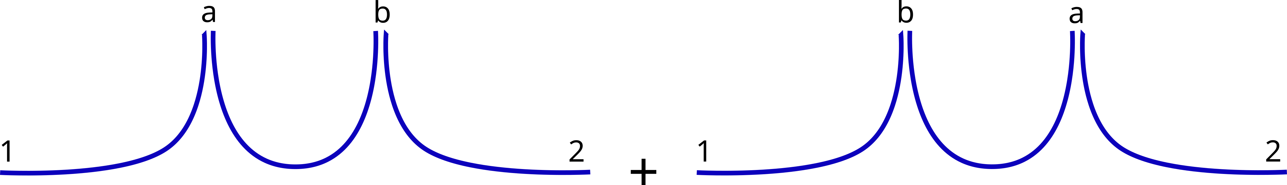
Figure 2: The large-$N_{c}$ colour-flow decomposition of the double real squared amplitude.

The colour-ordered double soft squared amplitude at tree level can be found in Section 5.3 of Ref. Campbell:1997hg (see also Section 8.1 of Ref. GehrmannDeRidder:2005cm ) and it is reported below 

$$\tilde{w}^{(0)}_{12}(k_{a},k_{b}) =2\,(2\pi)^{4}\mu^{4\epsilon}\bigg{[}\frac{s_{12}^{2}}{s_{1a}s_{ab2}s_{1ab}s_{b2}}+\frac{1-\epsilon}{s_{ab}^{2}}\left(\frac{s_{1a}}{s_{1ab}}+\frac{s_{b2}}{s_{ab2}}-1\right)^{2}$$

$$+\frac{s_{12}}{s_{ab}}\left(\frac{1}{s_{1a}s_{b2}}+\frac{1}{s_{1a}s_{ab2}}+\frac{1}{s_{b2}s_{1ab}}-\frac{4}{s_{1ab}s_{ab2}}\right)\bigg{]}\,,$$ (36)

where the Lorentz invariants $s_{i\dots k}$ indicate the standard Mandelstam variables. For later use, it is also convenient to single out the independent emission contribution and write

$$\tilde{w}^{(0)}_{12}(k_{a},k_{b})=\frac{1}{2}w^{(0)}_{12}(k_{a})w^{(0)}_{12}(k_{b})+\bar{w}^{(gg)}_{12}(k_{a},k_{b})\,.$$ (37)

Note, however, that the separation of the independent contribution is immaterial at the level of the single colour flow, and only makes physical sense at the level of the sum $\tilde{w}^{(0)}_{12}(k_{a},k_{b})+\tilde{w}^{(0)}_{12}(k_{b},k_{a})$. We also observe that the correlated term $\bar{w}^{(gg)}_{12}$ is not positive definite. The separation (37) is useful since the independent emission contribution is correctly described by the BMS equation as it simply arises from the iteration of the leading order squared amplitude. We can therefore focus on the correlated term of Eq. (37) in what follows.

The dipole structure of this double-real correction can be read from the last two terms of Eq. (4). In that equation, the first line corresponds to the usual dipole structure of the BMS equation, obtained from the replacement

$$\Delta_{1a}(k_{ta})\Delta_{a2}(k_{ta})\to~{}G_{1a}[k_{ta};u]G_{a2}[k_{ta};u]\,.$$ (38)

Similarly, the product of three Sudakov factors in the third and fifth line encodes the no-emission probability for the three dipoles created by the emission of $k_{a}$ and $k_{b}$ off the initial dipole $\{12\}$. The dipole structure for the double real correction then corresponds to replacing

$$\Delta_{1b}(k_{tb})\Delta_{ba}(k_{tb})\Delta_{a2}(k_{ta})\,\to~{} G_{1b}[k_{tb};u]G_{ba}[k_{tb};u]G_{a2}[k_{ta};u]\,,$$

$$\Delta_{1a}(k_{ta})\Delta_{ab}(k_{tb})\Delta_{b2}(k_{tb})\,\to~{} G_{1a}[k_{ta};u]G_{ab}[k_{tb};u]G_{b2}[k_{tb};u]\,.$$ (39)

As a last step, we need to upgrade the phase space boundary given by $\Theta(Q-k_{ta})$ in Eq. (4) which emerges from the strongly ordered limit. Conversely, the double real correction given by $\bar{w}^{(gg)}_{12}$ describes the emission of two gluons with commensurate $k_{t}$ (and energy) with respect of the emitting $\{12\}$ dipole. As a consequence, the definition of the resolution scale $Q$ used in Eq. (12) now has to constrain the total energy of $k_{a}+k_{b}$ or equivalently its transverse momentum w.r.t. the $\{12\}$ dipole, in order for the evolution to be collinear safe for any value of $Q$. In line with our choice of the dipole transverse momentum as evolution scale, we therefore perform the replacement

$$\Theta(Q-k_{ta})\to\Theta(Q-k_{t(ab)})\,,$$ (40)

where we defined

$$\vec{k}_{t(ab)}=\vec{k}_{ta}+\vec{k}^{\prime}_{tb}\,,$$ (41)

and $k_{t(ab)}=|\vec{k}_{t(ab)}|$. We denoted by $\vec{k}^{\prime}_{tb}$ the transverse momentum of $k_{b}$ with respect to the $\{12\}$ dipole and

$$(\vec{k}^{\prime}_{tb})^{2}=2\frac{(p_{1}\cdot k_{b})(p_{2}\cdot k_{b})}{(p_{1}\cdot p_{2})}\,.$$ (42)

Notice that $k^{\prime}_{tb}$ differs significantly from $k_{tb}$ (in the frame of the emitting dipole of $k_{b}$) in the limit in which $k_{b}$ is collinear to $k_{a}$, and the two have comparable energies. As already stressed, and we will show shortly, in this limit the real correction will cancel against the virtual contributions and therefore this limit is irrelevant for the observable considered here. In this case, one can only receive a NLL correction from the regime where $k^{\prime}_{tb}\sim k_{tb}$. Subtracting the double counting with the iteration of the BMS equation (4) leads to the following term to be added to the right hand side of Eq. (25)

$$\int[dk_{a}]\int[dk_{b}] \bar{\alpha}(k_{ta})\bar{\alpha}(k_{tb})\frac{\Delta_{12}(Q)}{\Delta_{12}(k_{ta})}\frac{\Delta_{1a}(k_{ta})}{\Delta_{1a}(k_{tb})}G_{1b}[k_{tb};u]G_{ba}[k_{tb};u]G_{a2}[k_{ta};u]u(k_{a})u(k_{b})$$

$$\times\,\left(\bar{w}^{(gg)}_{12}(k_{b},k_{a})\Theta(Q-k_{t(ab)})\Theta(k_{ta}-k_{tb}^{\prime})\right.$$

$$\qquad\qquad-\left.w^{(0)}_{12}(k_{a})\left(w^{(0)}_{1a}(k_{b})-\frac{1}{2}w^{(0)}_{12}(k_{b})\right)\Theta(Q-k_{ta})\Theta(k_{ta}-k_{tb})\right)$$

$$+\int[dk_{a}]\int[dk_{b}] \bar{\alpha}(k_{ta})\bar{\alpha}(k_{tb})\frac{\Delta_{12}(Q)}{\Delta_{12}(k_{ta})}\frac{\Delta_{a2}(k_{ta})}{\Delta_{a2}(k_{tb})}G_{1a}[k_{ta};u]G_{ab}[k_{tb};u]G_{b2}[k_{tb};u]u(k_{a})u(k_{b})$$

$$\times\left(\bar{w}^{(gg)}_{12}(k_{a},k_{b})\Theta(Q-k_{t(ab)})\Theta(k_{ta}-k_{tb}^{\prime})\right.$$ (43)

$$\qquad\qquad-\left.w^{(0)}_{12}(k_{a})\left(w^{(0)}_{a2}(k_{b})-\frac{1}{2}w^{(0)}_{12}(k_{b})\right)\Theta(Q-k_{ta})\Theta(k_{ta}-k_{tb})\right)\,,$$

where the two emissions are ordered in their dipole $k_{t}$. In its present form, Eq. (4) cannot be readily interpreted as a correction to the kernel of the evolution equation (25), in that it contains the product of two ratios of Sudakov factors that already indicate an iteration of the kernel. In order to derive a corresponding term at the level of the integral equation (25) we will need to make some considerations. As a next step we discuss virtual corrections at NLL order. The BMS equation already contains virtual corrections in the strongly ordered soft limit. However, these do not cancel the collinear singularity present in Eq. (4) when $k_{a}$ is collinear to $k_{b}$. For this, we need first to introduce the full one-loop corrections to the evolution kernel in the soft limit.

Virtual corrections.

The second term to consider is the virtual one-loop correction to the leading order kernel in the r.h.s. of Eq. (25). The structure of the virtual corrections can be read off the first line of Eq. (4). In the large-$N_{c}$ limit, the emission of $k_{a}$ generates two adjacent colour dipoles that emit further radiation incoherently. Therefore, the singularity structure of virtual corrections to the $\{1a2\}$ configuration will factorise into the product of virtual corrections to the $\{1a\}$ and $\{a2\}$ dipoles in this limit (see e.g. Gardi:2009qi ). This factorising structure is already encoded at LL in the first line of Eq. (4), specifically in the product $\Delta_{1a}(k_{ta})\Delta_{a2}(k_{ta})$. However, the LL Sudakov of factors in this product do not contain the correct NLL singular structure (i.e. the single poles), and therefore we need to supplement the first line of Eq. (4) with an extra correction factor that accounts for the missing terms.

The one loop corrections to the emission of the soft gluon $k_{a}$ off the $\{12\}$ dipole can be written as Catani:2000pi ; Angeles-Martinez:2016dph (given here in the large-$N_{c}$ limit)

$$w^{(1)}_{12}(k_{a})=w^{(0)}_{12}(k_{a})\left[V_{12}^{(1)}(\epsilon)-N_{c}\frac{\alpha_{s}}{\pi}\,\frac{(4\pi)^{\epsilon}}{2\epsilon^{2}}\frac{\Gamma^{4}(1-\epsilon)\Gamma^{3}(1+\epsilon)}{\Gamma^{2}(1-2\epsilon)\Gamma(1+2\epsilon)}\left(\frac{\mu^{2}}{k_{ta}^{2}}\right)^{\epsilon}\right]\,,$$ (44)

where $V_{12}^{(1)}(\epsilon)$ corresponds to one loop virtual corrections to the dipole $\{12\}$, while the second term encodes the one loop soft gluon current. In this context, the quantity $V_{12}^{(1)}(\epsilon)$ is not the full virtual correction to the Born process, but rather the virtual correction as predicted by the LL evolution equation. We derive this by using the unitarity of $G_{12}$ (cf. Eq. (26)), and expanding the Sudakov $\Delta(k_{ta})$ at ${\cal O}(\bar{\alpha})$, obtaining

$$V_{12}^{(1)}(\epsilon)=-\bar{\alpha}(\mu)\,\int[dk_{b}]w^{(0)}_{12}(k_{b})\Theta(Q-k_{tb})\,.$$ (45)

The mismatch between Eq. (45) and the full virtual correction to the Born process considered here is taken into account in the hard matching coefficient ${\cal H}_{2}$ computed in Sec. 5. Moreover, from Eq. (44) we also see that choosing $\mu=k_{ta}$ absorbs all the $k_{ta}$ dependence into the running coupling. Renormalising the coupling in the $\overline{\rm MS}$ scheme (cf. Eq. (15)) allows us to write

$$w^{(1)}_{12}(k_{a})\to-\bar{\alpha}(k_{ta})\,w^{(0)}_{12}(k_{a})\\ \times\left[\int[dk_{b}]\,\,w^{(0)}_{12}(k_{b})\Theta(Q-k_{tb})+\frac{e^{\epsilon\gamma_{E}}}{2\epsilon^{2}}\frac{\Gamma^{4}(1-\epsilon)\Gamma^{3}(1+\epsilon)}{\Gamma^{2}(1-2\epsilon)\Gamma(1+2\epsilon)}+\frac{\bar{\beta}_{0}}{\epsilon}\right]\,,$$ (46)

where $\bar{\beta}_{0}$ is defined by the coefficient of $N_{c}/\pi$ in the large-$N_{c}$ $\beta_{0}$ given in Eq. (16).

The virtual corrections to the evolution kernel are then obtained from the first line of Eq. (4) via the replacement

$$\frac{\Delta_{12}(Q)}{\Delta_{12}(k_{ta})}\Delta_{1a}(k_{ta})\Delta_{a2}(k_{ta})\to~{}\left(1+\bar{\alpha}(k_{ta})\gamma(k_{a},\epsilon)\right)\,\frac{\Delta_{12}(Q)}{\Delta_{12}(k_{ta})}\Delta_{1a}(k_{ta})\Delta_{a2}(k_{ta})\,,$$ (47)

where the function $\gamma(k_{a},\epsilon)$ determines the matching coefficient necessary to obtain the correct virtual corrections to the emission of a soft gluon. It is obtained by matching Eq (46) and the one-loop contribution to the r.h.s. of Eq. (47). The expansion of the r.h.s. of Eq. (47) gives

$$w^{(0)}_{12}(k_{a}) \left(1+\bar{\alpha}(k_{ta})\gamma(k_{a},\epsilon)\right)\,\frac{\Delta_{12}(Q)}{\Delta_{12}(k_{ta})}\Delta_{1a}(k_{ta})\Delta_{a2}(k_{ta})=w^{(0)}_{12}(k_{a})\left(1+\bar{\alpha}(k_{ta})\gamma(k_{a},\epsilon)\right)$$

$$-\bar{\alpha}(k_{ta})\,w^{(0)}_{12}(k_{a})\,\int[dk_{b}]\left[\left(w^{(0)}_{1a}(k_{b})+w^{(0)}_{a2}(k_{b})-w^{(0)}_{12}(k_{b})\right)\Theta(k_{ta}-k_{tb})\right.$$

$$\left.+\,w^{(0)}_{12}(k_{b})\Theta(Q-k_{tb})\right]+{\cal O}(\bar{\alpha}^{2}(k_{ta}))\,.$$ (48)

The coefficient of ${\cal O}(\bar{\alpha})$ in the above equation has to be matched to the one-loop expansion of Eq. (46), from which we obtain

$$\gamma(k_{a},\epsilon) =-\frac{e^{\epsilon\gamma_{E}}}{2\epsilon^{2}}\frac{\Gamma^{4}(1-\epsilon)\Gamma^{3}(1+\epsilon)}{\Gamma^{2}(1-2\epsilon)\Gamma(1+2\epsilon)}-\frac{\bar{\beta}_{0}}{\epsilon}$$

$$+\int[dk_{b}]\left(w^{(0)}_{1a}(k_{b})+w^{(0)}_{a2}(k_{b})-w^{(0)}_{12}(k_{b})\right)\Theta(k_{ta}-k_{tb})\,.$$ (49)

The last integral reads

$$\int[dk_{b}]\left(w^{(0)}_{1a}(k_{b})+w^{(0)}_{a2}(k_{b})-w^{(0)}_{12}(k_{b})\right)\Theta(k_{ta}-k_{tb})=\left(\frac{\mu^{2}}{k_{ta}^{2}}\right)^{\epsilon}\left(\frac{1}{2\epsilon^{2}}-\frac{\pi^{2}}{24}+{\cal O}(\epsilon)\right)\,,$$ (50)

which gives (setting $\mu=k_{ta}$)

$$\gamma(k_{a},\epsilon)=\gamma(\epsilon)=-\frac{11}{12\epsilon}+\frac{\pi^{2}}{6}+{\cal O}(\epsilon)\,.$$ (51)

Cancellation of collinear singularities.

We now combine the real and virtual corrections obtained above into a single integral equation in $d=4-2\epsilon$ dimensions. We want to achieve a manifest cancellation of soft and collinear singularities between real and virtual contributions independently of the precise form of the source $u(k)$. For this, we make use of the fact that, as stressed earlier, the double-real corrections of Eq. (4) only contribute in the unordered regime where $\omega_{a}\sim\omega_{b}$. For the observables considered in this article, this also implies $k_{ta}\sim k_{tb}\sim k_{t(ab)}$. To see this, we observe that $k_{ta}\sim k_{tb}$ only if $\omega_{a}\sim\omega_{b}$ and the two gluons are not collinear to one another. Away from this configuration, when the two gluons become collinear, one can end up in a situation with $\omega_{a}\sim\omega_{b}$ but the dipole transverse momenta are strongly ordered, i.e. $k_{ta}\gg k_{tb}$. This configuration however only contributes to the observable if both gluons are inside the rapidity slice, hence at wide angles w.r.t. the $\{12\}$ dipole, and the corresponding collinear singularity exactly cancels against the one in $\gamma(\epsilon)$ (51) at all orders in $\bar{\alpha}$, leaving behind only finite contribution without a logarithmic enhancement (i.e. NNLL). Conversely, for an observable sensitive also to collinear radiation (e.g. the light-hemisphere mass), this configuration can occur with both soft gluons being simultaneously collinear to one of the $\{12\}$ dipole ends, and to each other. The singularity structure of this configuration would result in an extra logarithmic enhancement and the argument made above would not hold. This extra logarithmic enhancement can be however resummed by means of standard techniques used for global observables, and the formalism presented here can still be used for the calculation of the non-global contributions. We can therefore perform a first-order Taylor expansion and make the following approximation in the double real corrections given in Eq. (4)

$$\bar{\alpha}(k_{ta})\bar{\alpha}(k_{tb})\frac{\Delta_{12}(Q)}{\Delta_{12}(k_{ta})}\frac{\Delta_{1a}(k_{ta})}{\Delta_{1a}(k_{tb})}\sim\bar{\alpha}^{2}(k_{ta})\frac{\Delta_{12}(Q)}{\Delta_{12}(k_{ta})}\sim\bar{\alpha}^{2}(k_{t(ab)})\frac{\Delta_{12}(Q)}{\Delta_{12}(k_{t(ab)})}\,,$$ (52)

(and similarly for the second term corresponding to the alternative colour flow) where we systematically neglected corrections of order

$${\cal O}\left(\alpha_{s}\ln k_{ta}/k_{t(ab)}\right)\sim{\cal O}\left(\alpha_{s}\ln k_{ta}/k_{tb}\right)\sim{\cal O}\left(\alpha_{s}\right)\sim{\cal O}\left({\rm NNLL}\right)\,,$$ (53)

in the limit of soft-wide-angle radiation. This is because the logarithm of the ratios $k_{ta}/k_{t(ab)}$ and $k_{ta}/k_{tb}$ are not large in the region where Eq. (4) is non vanishing, and the quantity (53) only gives a contribution of ${\cal O}(1)$ upon integration over the phase space of $k_{a}$ and $k_{b}$, that is a NNLL correction. We can write the NLL integral equation in $d$ dimensions as

$$G_{12}[Q;u]=\Delta_{12}(Q)+\int[dk_{a}]\bar{\alpha}(k_{ta})w^{(0)}_{12}(k_{a})\,\bigg{(}1+\bar{\alpha}(k_{ta})\,\gamma(\epsilon)\bigg{)}$$ (54)

$$\times\frac{\Delta_{12}(Q)}{\Delta_{12}(k_{ta})}G_{1a}[k_{ta};u]G_{a2}[k_{ta};u]u(k_{a})\Theta(Q-k_{ta})$$

$$+\int[dk_{a}]\int[dk_{b}]\bar{\alpha}^{2}(k_{t(ab)})\frac{\Delta_{12}(Q)}{\Delta_{12}(k_{t(ab)})}u(k_{a})u(k_{b})\Theta(Q-k_{t(ab)})\Theta(k_{ta}-k_{tb}^{\prime})$$

$$\times\left[\bar{w}^{(gg)}_{12}(k_{b},k_{a})G_{1b}[k_{t(ab)};u]G_{ba}[k_{t(ab)};u]G_{a2}[k_{t(ab)};u]\right.$$

$$\left.\hskip 85.35826pt+\bar{w}^{(gg)}_{12}(k_{a},k_{b})G_{1a}[k_{t(ab)};u]G_{ab}[k_{t(ab)};u]G_{b2}[k_{t(ab)};u]\right]$$

$$-\int[dk_{a}]\int[dk_{b}]\bar{\alpha}^{2}(k_{ta})\frac{\Delta_{12}(Q)}{\Delta_{12}(k_{ta})}u(k_{a})u(k_{b})\Theta(Q-k_{ta})\Theta(k_{ta}-k_{tb})$$

$$\times\left[w^{(0)}_{12}(k_{a})\left(w^{(0)}_{1a}(k_{b})-\frac{1}{2}w^{(0)}_{12}(k_{b})\right)G_{1b}[k_{ta};u]G_{ba}[k_{ta};u]G_{a2}[k_{ta};u]\right.$$

$$\left.\hskip 85.35826pt+w^{(0)}_{12}(k_{a})\left(w^{(0)}_{a2}(k_{b})-\frac{1}{2}w^{(0)}_{12}(k_{b})\right)G_{1a}[k_{ta};u]G_{ab}[k_{ta};u]G_{b2}[k_{ta};u]\right]\,,$$

where we have also Taylor expanded the scale of $G_{12}$ in the double real correction following the same argument as in Eq. (53). We will shortly discuss a way to make the subtraction of IRC divergences manifest and eventually to take the limit $\epsilon\to 0$.

The NLL Sudakov form factor.

As a consistency check of the above equation, we can use Eq. (54) to derive the NLL soft anomalous dimension that enters the evolution equation of the soft corrections to the Sudakov form factor given in Ref. Magnea:2000ss . We start by setting the source $u$ to 1 (hence $G[1]=1$) in Eq. (54) and obtain

$$1= \Delta_{12}(Q)+\int[dk_{a}]\bar{\alpha}(k_{ta})w^{(0)}_{12}(k_{a})\,\bigg{(}1+\bar{\alpha}(k_{ta})\,\gamma(\epsilon)\bigg{)}\frac{\Delta_{12}(Q)}{\Delta_{12}(k_{ta})}\Theta(Q-k_{ta})$$

$$+\int[dk_{a}]\int[dk_{b}]\bar{\alpha}^{2}(k_{t(ab)})\frac{\Delta_{12}(Q)}{\Delta_{12}(k_{t(ab)})}\Theta(Q-k_{t(ab)})\Theta(k_{ta}-k_{tb}^{\prime})$$

$$\times\left[\bar{w}^{(gg)}_{12}(k_{b},k_{a})+\bar{w}^{(gg)}_{12}(k_{a},k_{b})\right]$$

$$-\int[dk_{a}]\int[dk_{b}]\bar{\alpha}^{2}(k_{ta})\frac{\Delta_{12}(Q)}{\Delta_{12}(k_{ta})}\Theta(Q-k_{ta})\Theta(k_{ta}-k_{tb})$$

$$\times w^{(0)}_{12}(k_{a})\left(w^{(0)}_{1a}(k_{b})+w^{(0)}_{a2}(k_{b})-w^{(0)}_{12}(k_{b})\right)\,.$$ (55)

We now introduce a $d$-dimensional massless momentum $k$ such that $k_{t}\coloneqq|\vec{k}_{t}|=k_{t(ab)}$ and its rapidity $\eta$ with respect to the emitting dipole $\{12\}$ is that of the $k_{a}+k_{b}$ system $\eta_{(ab)}$, this is defined by the corresponding kinematic map

$${\mathbb{P}}:\{k_{a},k_{b}\}\rightarrow k_{(ab)}=\left(k_{t(ab)}\cosh\eta_{(ab)},\vec{k}_{t(ab)},k_{t(ab)}\sinh\eta_{(ab)}\right)\,,$$ (56)

where the three-vectors are taken in the rest frame of the $\{12\}$ dipole. We recast the above equation as

$$1= \Delta_{12}(Q)+\int[dk_{a}]\bar{\alpha}(k_{ta})w^{(0)}_{12}(k_{a})\,\bigg{(}1+\bar{\alpha}(k_{ta})\,\gamma(\epsilon)\bigg{)}\frac{\Delta_{12}(Q)}{\Delta_{12}(k_{ta})}\Theta(Q-k_{ta})$$

$$+\int[dk]\,\bar{\delta}(k-k_{a}-k_{b})\bar{\alpha}^{2}(k_{t})\frac{\Delta_{12}(Q)}{\Delta_{12}(k_{t})}\Theta(Q-k_{t})$$

$$\times\int[dk_{a}]\int[dk_{b}]\Theta(k_{ta}-k_{tb}^{\prime})\left(\bar{w}^{(gg)}_{12}(k_{b},k_{a})+\bar{w}^{(gg)}_{12}(k_{a},k_{b})\right)$$

$$-\int[dk_{a}]\int[dk_{b}]\bar{\alpha}^{2}(k_{ta})\frac{\Delta_{12}(Q)}{\Delta_{12}(k_{ta})}\Theta(Q-k_{ta})\Theta(k_{ta}-k_{tb})$$

$$\times w^{(0)}_{12}(k_{a})\left(w^{(0)}_{1a}(k_{b})+w^{(0)}_{a2}(k_{b})-w^{(0)}_{12}(k_{b})\right)\,,$$ (57)

where we defined

$$\bar{\delta}(k-k_{a}-k_{b})\coloneqq 2(2\pi)^{3-2\epsilon}\delta^{(2-2\epsilon)}(\vec{k}_{t}-\vec{k}_{ta}-\vec{k}^{\prime}_{tb})\delta(\eta-\eta_{(ab)})\,.$$ (58)

We now divide Eq. (4) by $\Delta_{12}(Q)$ and take the derivative with respect to $\ln Q$, obtaining the differential evolution equation

$$\frac{d\ln\Delta_{12}(Q)}{d\ln Q}=-\int[dk]Q\delta(Q-k_{t})\bigg{\{}\bar{\alpha}(k_{t})w^{(0)}_{12}(k)\,\bigg{(}1+\bar{\alpha}(k_{t})\,\gamma(\epsilon)\bigg{)}$$ (59)

$$+\bar{\alpha}^{2}(k_{t})\int[dk_{a}]\int[dk_{b}]\bar{\delta}(k-k_{a}-k_{b})\bigg{[}\,\bar{w}^{(gg)}_{12}(k_{b},k_{a})+\bar{w}^{(gg)}_{12}(k_{a},k_{b})\bigg{]}\Theta(k_{ta}-k_{tb}^{\prime})$$

$$-\bar{\alpha}^{2}(k_{t})\int[dk_{a}]\int[dk_{b}]\bar{\delta}(k-k_{a})\left[w^{(0)}_{12}(k_{a})\left(w^{(0)}_{1a}(k_{b})+w^{(0)}_{a2}(k_{b})-w^{(0)}_{12}(k_{b})\right)\right]\Theta(k_{ta}-k_{tb})\bigg{\}}\,.$$

In the second line of Eq. (59), it is convenient to parametrise the double real phase space as in Dokshitzer:1997iz (see also Ref. Banfi:2018mcq for the $d$-dimensional case)

$$[dk_{a}][dk_{b}]=[dk]\frac{dz[z(1-z)]^{-\epsilon}}{(4\pi)^{2}}\frac{dm_{ab}^{2}}{m_{ab}^{2\epsilon}}\frac{d\Omega_{2-2\epsilon}}{(2\pi)^{1-2\epsilon}}\,,$$ (60)

where $[dk]$ is given in Eq. (22), $m_{ab}^{2}=(k_{a}+k_{b})^{2}\in[0,\infty)$, and $z\in[0,1]$ is the fraction of one of the light cone components of $k$ with respect to the $\{12\}$ dipole carried by one of the daughters $k_{a}$ or $k_{b}$. For instance if we adopt the following Sudakov parametrisation for the four momenta

$$k_{a/b}^{\mu} =z_{a/b}^{(1)}\,p_{1}^{\mu}+z_{a/b}^{(2)}\,p_{2}^{\mu}+\kappa_{{a/b}}^{\mu}$$

$$k^{\mu} =z^{(1)}\,p_{1}^{\mu}+z^{(2)}\,p_{2}^{\mu}+\kappa^{\mu}\,,$$ (61)

with $\kappa_{i}$ being a space-like transverse vector describing the transverse momentum of $k_{i}$ w.r.t. the $\{12\}$ dipole, we can define $z$ as

$$z_{a}^{(1)}=z\,z^{(1)}\,\quad z_{b}^{(1)}=(1-z)\,z^{(1)}\,.$$ (62)

Finally, $d\Omega_{2-2\epsilon}$ is the angular phase space for the vector $\vec{q}\coloneqq\frac{\vec{k}_{ta}}{z}-\frac{\vec{k}^{\prime}_{tb}}{1-z}$ with respect to $\vec{k}_{t}$, given by

$$\frac{d\Omega_{2-2\epsilon}}{(2\pi)^{1-2\epsilon}}=\frac{(4\pi)^{\epsilon}}{\sqrt{\pi}\Gamma(\frac{1}{2}-\epsilon)}d\phi\,(\sin^{2}\phi)^{-\epsilon}\,,\qquad\phi\in[0,\pi]\,.$$ (63)

Since $k$ is massless, we can integrate inclusively over $m_{ab}$ in the second line of Eq. (59), and find

$$\int[dk_{a}]\int[dk_{b}]\,\bar{\delta}(k-k_{a}-k_{b})\bigg{[}\,\bar{w}^{(gg)}_{12}(k_{b},k_{a})+\bar{w}^{(gg)}_{12}(k_{a},k_{b})\bigg{]}\Theta(k_{ta}-k_{tb}^{\prime})$$

$$\qquad=w^{(0)}_{12}(k)\left(\frac{\mu^{2}}{k_{t}^{2}}\right)^{\epsilon}\left(\frac{1}{2\epsilon^{2}}+\frac{11}{12\epsilon}+\frac{67}{36}-\frac{7}{24}\pi^{2}+{\cal O}(\epsilon)\right)\,,$$ (64)

$$\int[dk_{a}]\int[dk_{b}]\,\bar{\delta}(k-k_{a})\left[w^{(0)}_{12}(k_{a})\left(w^{(0)}_{1a}(k_{b})+w^{(0)}_{a2}(k_{b})-w^{(0)}_{12}(k_{b})\right)\right]\Theta(k_{ta}-k_{tb})$$

$$\qquad=w^{(0)}_{12}(k)\left(\frac{\mu^{2}}{k_{t}^{2}}\right)^{\epsilon}\left(\frac{1}{2\epsilon^{2}}-\frac{\pi^{2}}{24}+{\cal O}(\epsilon)\right)\,.$$ (65)

This leads to the well known evolution equation for the soft radiative corrections to the Sudakov form factor (see e.g. Laenen:2000ij ; Magnea:2000ss ; Dixon:2008gr ), which can be expressed as Laenen:2000ij ; Banfi:2018mcq

$$\frac{d\ln\Delta_{12}(Q)}{d\ln Q}=-\int[dk]Q\delta(Q-k_{t})\bar{\alpha}(k_{t})w^{(0)}_{12}(k)\left(1+\bar{\alpha}(k_{t})\bar{K}^{(1)}+{\cal O}(\bar{\alpha}^{2}(k_{t}))\right)\,,$$ (66)

where

$$\bar{K}^{(1)}=\frac{67}{36}-\frac{\pi^{2}}{12}$$ (67)

is the coefficient of $N_{c}$ of the large-$N_{c}$ two-loop cusp anomalous dimension in units of $\alpha_{s}/\pi$. One can directly use this result and Eq. (54) to derive a differential equation for $G_{12}$ in $d$ dimensions. However, since we are ultimately interested in a numerical evaluation of its solution, we first discuss how to take the limit $\epsilon\to 0$.

4.1 The NLL differential equation

In order to take the $\epsilon\to 0$ limit we wish to make the cancellation of infrared singularities in Eq. (54) manifest. This is crucial to solve the evolution equation numerically for different infrared safe observables. To this end we introduce the counterterm

$$\int[dk_{a}]\int[dk_{b}]\bar{\alpha}^{2}(k_{t(ab)})\frac{\Delta_{12}(Q)}{\Delta_{12}(k_{t(ab)})}u(k_{(ab)})\Theta(Q-k_{t(ab)})\Theta(k_{ta}-k_{tb}^{\prime})$$

$$\qquad\times\left[\bar{w}^{(gg)}_{12}(k_{b},k_{a})+\bar{w}^{(gg)}_{12}(k_{a},k_{b})\right]G_{1(ab)}[k_{t(ab)};u]G_{(ab)2}[k_{t(ab)};u]$$

$$-\int[dk_{a}]\int[dk_{b}]\bar{\alpha}^{2}(k_{ta})\frac{\Delta_{12}(Q)}{\Delta_{12}(k_{ta})}u(k_{a})\Theta(Q-k_{ta})\Theta(k_{ta}-k_{tb})$$

$$\qquad\times\left[w^{(0)}_{12}(k_{a})\left(w^{(0)}_{1a}(k_{b})+w^{(0)}_{12}(k_{a})-w^{(0)}_{12}(k_{b})\right)\right]G_{1a}[k_{ta};u]G_{a2}[k_{ta};u]\,.$$ (68)

which we add and subtract to Eq. (54). The main difference between Eq. (4.1) and the double real correction (4) is the source evaluated on the massless momentum $k_{(ab)}$ defined in Eq. (56). This definition, owing to the collinear safety of source $u(k)$ in Eq. (4.1), guarantees that the collinear singularity is consistently cancelled in the difference between the double-real contribution to Eq. (54) and the counterterm (4.1). In general, one can replace the momentum $k_{(ab)}$ with the result of any kinematic map ${\mathbb{P}}:\{k_{a},k_{b}\}\rightarrow k_{(ab)}$ such that in the limit where $k_{a}$ and $k_{b}$ are collinear, the transverse momentum and rapidity of the $k_{(ab)}$ momentum coincide with those of the $k_{a}+k_{b}$ system with respect to the $\{12\}$ dipole. The choice of the kinematic map used in the subtraction is arbitrary, and here we adopt the massless projection of Eq. (56) since it makes the computation of the integrated counterterm simple.

A second important difference between Eq. (4.1) and Eq. (4) is that the generating functionals $G_{1(ab)}$ and $G_{(ab)2}$ now depend on the angle of the momentum $k_{(ab)}$ with respect to the $\{12\}$ dipole defined by the above projection (56). We now deal with the integral of the counterterm (4.1), which is instead combined with the real-virtual corrections in the first two lines of Eq. (54). Given the massless nature of $k_{(ab)}$, we can adopt the parametrisation (60) and integrate as in Eq. (4). The integrated counterterm then cancels the $\epsilon$ poles of $\gamma(\epsilon)$ in Eq. (54), and will later allow us to take the limit $\epsilon\to 0$ at the integrand level. One can finally derive the corresponding integro-differential equation, and bring it in the form given in Eq. (3.2). As done for the evolution equation for the NLL Sudakov factor, we start by dividing Eq. (54) supplemented with the counterterm introduced above by $\Delta_{12}(Q)$ and then we take the derivative with respect to $\ln Q$. Using the evolution equation for the Sudakov factor (66) one finds that the dependence on the Sudakov factors entirely drops out and we obtain the NLL evolution equation

$$Q\partial_{Q}G_{12}[Q;u] ={\mathbb{K}}^{\rm NLL}[G[Q,u],u]$$

$$\coloneqq{\mathbb{K}}^{\rm RV+VV}[G[Q,u],u]+{\mathbb{K}}^{\rm RR}[G[Q,u],u]-{\mathbb{K}}^{\rm DC}[G[Q,u],u]\,.$$ (69)

where we have defined

$${\mathbb{K}}^{\rm RV+VV} [G[Q,u],u]\coloneqq\int[dk_{a}]\bar{\alpha}(Q)w^{(0)}_{12}(k_{a})\,\bigg{(}1+\bar{\alpha}(Q)\,\bar{K}^{(1)}\bigg{)}$$ (70)

$$\hskip 28.45274pt\times\left(G_{1a}[Q;u]G_{a2}[Q;u]u(k_{a})-G_{12}[Q;u]\right)Q\delta(Q-k_{ta})\,,$$

as the kernel correction due to the virtual and subtracted real-virtual corrections,

$${\mathbb{K}}^{\rm RR} [G[Q,u],u]\coloneqq\int[dk_{a}]\int[dk_{b}]\,\bar{\alpha}^{2}(Q)Q\delta(Q-k_{t(ab)})\Theta(k_{ta}-k_{tb}^{\prime})$$ (71)

$$\times\left[\bar{w}^{(gg)}_{12}(k_{b},k_{a})G_{1b}[Q;u]G_{ba}[Q;u]G_{a2}[Q;u]u(k_{a})u(k_{b})\right.$$

$$\left.\hskip 28.45274pt+\bar{w}^{(gg)}_{12}(k_{a},k_{b})G_{1a}[Q;u]G_{ab}[Q;u]G_{b2}[Q;u]u(k_{a})u(k_{b})\right.$$

$$\left.\hskip 56.9055pt-\left(\bar{w}^{(gg)}_{12}(k_{b},k_{a})+\bar{w}^{(gg)}_{12}(k_{a},k_{b})\right)G_{1(ab)}[Q;u]G_{(ab)2}[Q;u]u(k_{(ab)})\right]\,,$$

for the double real corrections, and finally

$${\mathbb{K}}^{\rm DC} [G[Q,u],u]\coloneqq\int[dk_{a}]\int[dk_{b}]\bar{\alpha}^{2}(Q)Q\delta(Q-k_{ta})\Theta(k_{ta}-k_{tb})$$ (72)

$$\times\biggl{[}w^{(0)}_{12}(k_{a})\left(w^{(0)}_{1a}(k_{b})-\frac{1}{2}w^{(0)}_{12}(k_{b})\right)G_{1b}[Q;u]G_{ba}[Q;u]G_{a2}[Q;u]u(k_{a})u(k_{b})$$

$$\hskip 28.45274pt+w^{(0)}_{12}(k_{a})\left(w^{(0)}_{a2}(k_{b})-\frac{1}{2}w^{(0)}_{12}(k_{b})\right)G_{1a}[Q;u]G_{ab}[Q;u]G_{b2}[Q;u]u(k_{a})u(k_{b})$$

$$\hskip 56.9055pt-w^{(0)}_{12}(k_{a})\left(w^{(0)}_{1a}(k_{b})+w^{(0)}_{a2}(k_{b})-w^{(0)}_{12}(k_{b})\right)G_{1a}[Q;u]G_{a2}[Q;u]u(k_{a})\biggr{]}\,,$$

for the subtraction of the double counting with the iteration of the LL evolution kernel. In taking the four-dimensional limit in Eqs. (71) and (72), while keeping NLL contributions only, we implicitly neglect NNLL configurations in which $k_{a}$ and $k_{b}$ are both inside the rapidity slice. This is also crucial to guarantee the collinear safety of Eq. (72). Finally, we observe that since the observables under consideration are sensitive only to radiation at small rapidities, the exact rapidity bound (23) in the phase space integral is irrelevant. Therefore, it can be relaxed and set as

$$-\infty<\eta_{a/b}<+\infty$$ (73)

in the differential equations (31) and (4.1), which are both collinear safe and thus well defined since outside the slice there is a complete cancellation between real and virtual corrections. On the other hand, in the corresponding integral equations, virtual corrections are encoded in the Sudakov form factors. Therefore, one cannot use Eq. (73) since real and virtual terms require a finite rapidity upper bound in order to be separately well defined. In this case the initial rapidity bound (23) must be retained although the insensitivity of the observable to the large rapidity region ensures that the dependence on this cancels out eventually. The boundary conditions to Eq. (4.1) in $d$ dimensions are given in Eq. (19).

4.2 Limit to $d=4$ and boundary conditions

We now briefly comment on taking the $\epsilon\to 0$ limit of Eqs. (31) and (4.1). The right-hand side of both equations is now finite and well defined in four dimensions as long as the evolution scale is larger than $\Lambda_{\rm QCD}$, so that the limit $\epsilon\to 0$ can be directly taken at the integrand level. However, the boundary condition given in Eq. (19) is not well defined in this limit because of the Landau singularity. One has to supplement the evolution equations for $G_{12}$ with some non-perturbative modelling that allows the computation at very small scales. A simple prescription in the context of a numerical calculation is to introduce a freezing of the coupling at some small scale $Q_{0}>\Lambda_{\rm QCD}$ such that

$$\alpha_{s}(k)=\alpha_{s}(Q_{0}),\qquad k\leq Q_{0}\,.$$ (74)

An alternative prescription is to require that $G_{12}$ is kept constant below the freezing point $Q_{0}$, resulting in the boundary condition

$$G_{12}[Q;u]=1~{}{\rm for}~{}Q\leq Q_{0}\,,$$ (75)

while the unitarity condition $G_{12}[Q;1]=1$ is unchanged. The physical picture corresponding to Eq. (75) is that, below the resolution scale $Q_{0}$, real radiation cancels exactly virtual corrections by virtue of unitarity. This of course requires that the freezing scale $Q_{0}\ll v$, which is the typical scale of soft radiation inside the observed rapidity gap. If this condition is satisfied, the dependence on the infrared scale $Q_{0}$ becomes numerically negligible. In their four-dimensional formulation, Eqs. (20) and (4.1) can be evaluated numerically with the boundary conditions (74), or (75), either via discretisation techniques or by Monte Carlo methods. We will address the numerical solution in a forthcoming publication.

5 Computation of the one-loop hard matching factors

We now discuss the hard factors in Eq. (5). These account for the contribution of hard radiation that propagates outside of the observed region of phase space (rapidity slice in our case). Below we will give a definition that allows for a numerical implementation of the formulae derived in this article.

To extract the matching coefficients ${\cal H}_{2}$ and ${\cal H}_{3}$, it is instructive to see how they arise from an explicit NLO calculation in the case of $e^{+}e^{-}\to$ jets. We recall that here we use a flavour-based labelling of momenta, where $p_{1}$ and $p_{2}$ are the momenta of the quark and the antiquark, and $p_{3}$ the momentum of an additional hard gluon. The ${\cal O}(\alpha_{s})$ virtual contribution to the cumulative cross section reads (in the $\overline{\rm MS}$ scheme and with $\alpha_{s}=\alpha_{s}(\mu)$)

$$\Sigma^{{\rm virt.}}(v)=C_{F}\frac{\alpha_{s}}{2\pi}\left(\frac{\mu^{2}}{s}\right)^{\epsilon}\frac{e^{\gamma_{E}\epsilon}}{\Gamma(1-\epsilon)}\left(-\frac{2}{\epsilon^{2}}-\frac{3}{\epsilon}+\pi^{2}-8\right)S_{2}(v)\,.$$ (76)

To obtain the real corrections, and in order to avoid introducing additional abstract notation, we explicitly parametrise the phase space in terms of the energy fraction of the gluon $x\coloneqq 2E_{g}/\sqrt{s}$ and the cosine of the angle between the gluon and the quark $y\coloneqq\cos\theta_{qg}$, obtaining

$$\Sigma^{{\rm real}}(v)=2C_{F}\frac{\alpha_{s}}{2\pi}\left(\frac{\mu^{2}}{s}\right)^{\epsilon}\frac{e^{\gamma_{E}\epsilon}}{\Gamma(1-\epsilon)}\int_{0}^{1}dx\frac{x^{-1-2\epsilon}}{(1-x)^{2\epsilon}}\int_{-1}^{1}dy\,\frac{(1-y)^{-1-\epsilon}(1+y)^{-1-\epsilon}}{(2-x(1-y))^{2-2\epsilon}}$$

$$\times\left(8-\epsilon x^{2}(2-x(1-y))^{2}-(2-x)x\left((x-2)x(1-y)^{2}-4y+8\right)\right)\Theta_{\rm out}(k)S_{3}(v)\,.$$ (77)

The three directions $\vec{n}_{i}$ ($i=1,2,3$) in $S_{3}$ correspond to the directions of the quark, antiquark and gluon that are entirely specified by the variables $x$ and $y$. The phase space constraint $\Theta_{\rm out}(k)$ ensures that no hard parton is inside the observed rapidity slice, so that the observable is zero in a pure three-parton configuration. It can be entirely parametrised in terms of the kinematics of the gluon $k$. Configurations with a hard parton inside the slice would just correspond to power corrections and can be accounted for at fixed perturbative order through standard matching procedures. Upon integration over $x$ and $y$, Eq. (5) develops double and single poles in $\epsilon$ that exactly cancel against those in Eq. (76).

In order to derive the expressions for ${\cal H}_{2}$ and ${\cal H}_{3}$, we now need to subtract the double counting with the real and virtual corrections to the evolution equation at ${\cal O}(\alpha_{s})$. These can be derived from the results of the previous section. The virtual corrections are given in Eq. (45) and at ${\cal O}(\alpha_{s})$ read (we set the upper bound of the evolution scale $Q=\sqrt{s}$)

$$\Sigma^{{\rm virt.}}_{\rm soft}(v) =-4C_{F}\frac{\alpha_{s}}{2\pi}\mu^{2\epsilon}\frac{e^{\gamma_{E}\epsilon}}{\Gamma(1-\epsilon)}\int_{0}^{\sqrt{s}}\frac{dk_{t}}{k_{t}^{1+2\epsilon}}\int_{\ln(k_{t}/\sqrt{s})}^{\ln(\sqrt{s}/k_{t})}d\eta\,S_{2}(v)$$

$$\qquad=C_{F}\frac{\alpha_{s}}{2\pi}\left(\frac{\mu^{2}}{s}\right)^{\epsilon}\frac{e^{\gamma_{E}\epsilon}}{\Gamma(1-\epsilon)}\left(-\frac{2}{\epsilon^{2}}\right)S_{2}(v)\,.$$ (78)

Similarly, the real corrections can be obtained from the first iteration of the evolution equation (25), retaining only the contribution in which the soft gluon $k$ is outside the slice, obtaining

$$\Sigma^{{\rm real}}_{\rm soft}(v) =4C_{F}\frac{\alpha_{s}}{2\pi}\mu^{2\epsilon}\frac{e^{\gamma_{E}\epsilon}}{\Gamma(1-\epsilon)}\int_{0}^{\sqrt{s}}\frac{dk_{t}}{k_{t}^{1+2\epsilon}}\int_{\ln(k_{t}/\sqrt{s})}^{\ln(\sqrt{s}/k_{t})}d\eta\,S^{\rm soft}_{3}(v)\Theta^{\rm soft}_{\rm out}(k)\,,$$ (79)

where $S^{\rm soft}_{3}$ indicates that the gluon $k$ defining the third direction $\vec{n}_{3}$ is soft, so no recoil is present in the event kinematics. In the above equation $\Theta^{\rm soft}_{\rm out}(k)$ ensures again that no partons are present inside the slice at ${\cal O}(\alpha_{s})$. Its expression differs from that of $\Theta_{\rm out}(k)$ in that no kinematic recoil is present in the soft limit and therefore the thrust axis is aligned with the direction of the quark (antiquark).

From there, we can compute the hard contribution to the virtual corrections as

$$\Sigma^{{\rm virt.}}(v)-\Sigma^{{\rm virt.}}_{\rm soft}(v)=C_{F}\frac{\alpha_{s}}{2\pi}\left(\frac{\mu^{2}}{s}\right)^{\epsilon}\frac{e^{\gamma_{E}\epsilon}}{\Gamma(1-\epsilon)}\left(-\frac{3}{\epsilon}+\pi^{2}-8\right)S_{2}(v)\,,$$ (80)

which, as expected, contains only a single pole of hard-collinear nature. We now consider the difference between the real corrections given in Eqs. (5), (79). Before taking the difference, we observe that the phase space for the emission of a soft gluon in Eq. (79) is larger than the one imposed by momentum conservation in Eq. (5). This difference comes from having expanded consistently the rapidity boundary as in Eq. (23) as well as from taking $k_{t}\leq\sqrt{s}$ rather than $\sqrt{s}/2$ as required by energy conservation. We can therefore recast Eq. (79) as the sum of a term with the same phase-space limits as Eq. (5) and a remainder as

$$\Sigma^{{\rm real}}_{\rm soft}(v) =4C_{F}\frac{\alpha_{s}}{2\pi}\mu^{2\epsilon}\frac{e^{\gamma_{E}\epsilon}}{\Gamma(1-\epsilon)}\bigg{[}\int_{0}^{\frac{\sqrt{s}}{2}}\frac{dk_{t}}{k_{t}^{1+2\epsilon}}\int_{-\cosh^{-1}\frac{\sqrt{s}}{2k_{t}}}^{\cosh^{-1}\frac{\sqrt{s}}{2k_{t}}}d\eta+\int_{0}^{\sqrt{s}}\frac{dk_{t}}{k_{t}^{1+2\epsilon}}\int_{\ln\frac{k_{t}}{\sqrt{s}}}^{-\cosh^{-1}\frac{\sqrt{s}}{2k_{t}}}d\eta$$

$$+\int_{0}^{\sqrt{s}}\frac{dk_{t}}{k_{t}^{1+2\epsilon}}\int_{\cosh^{-1}\frac{\sqrt{s}}{2k_{t}}}^{\ln\frac{\sqrt{s}}{k_{t}}}d\eta+\int_{\frac{\sqrt{s}}{2}}^{\sqrt{s}}\frac{dk_{t}}{k_{t}^{1+2\epsilon}}\int_{-\cosh^{-1}\frac{\sqrt{s}}{2k_{t}}}^{\cosh^{-1}\frac{\sqrt{s}}{2k_{t}}}d\eta\bigg{]}S^{\rm soft}_{3}(v)\Theta^{\rm soft}_{\rm out}(k)\,.$$ (81)

For the first term we can now switch to the same $x$, $y$ variables used for Eq. (5)

$$\int_{0}^{\frac{\sqrt{s}}{2}}\frac{dk_{t}}{k_{t}^{1+2\epsilon}}\int_{-\cosh^{-1}\frac{\sqrt{s}}{2k_{t}}}^{\cosh^{-1}\frac{\sqrt{s}}{2k_{t}}}d\eta=4^{\epsilon}\,s^{-\epsilon}\int_{0}^{1}dx\,x^{-1-2\epsilon}\int_{-1}^{1}dy\,(1-y)^{-1-\epsilon}(1+y)^{-1-\epsilon}\,,$$ (82)

while the integrals in the second line of Eq. (5) are now finite and one can take the limit $\epsilon\to 0$ prior to integration. We can now take the difference between Eq. (5) and (5) and obtain

$$\Sigma^{{\rm real}}(v) -\Sigma^{{\rm real}}_{\rm soft}(v)=2C_{F}\frac{\alpha_{s}}{2\pi}\left(\frac{\mu^{2}}{s}\right)^{\epsilon}\frac{e^{\gamma_{E}\epsilon}}{\Gamma(1-\epsilon)}\int_{0}^{1}dx\,x^{-1-2\epsilon}\int_{-1}^{1}dy\,(1-y)^{-1-\epsilon}(1+y)^{-1-\epsilon}$$

$$\!\!\!\!\!\times\bigg{[}\frac{8-\left(\epsilon x^{2}(2-x(1-y))^{2}+(2-x)x\left((x-2)x(1-y)^{2}-4y+8\right)\right)}{(1-x)^{2\epsilon}(2-x(1-y))^{2-2\epsilon}}\Theta_{\rm out}(k)S_{3}(v)$$

$$\!\!\!\!\!-2^{1+2\epsilon}\Theta^{\rm soft}_{\rm out}(k)S^{\rm soft}_{3}(v)\bigg{]}$$

$$\!\!\!\!\!-4C_{F}\frac{\alpha_{s}}{2\pi}\bigg{[}\int_{0}^{\sqrt{s}}\frac{dk_{t}}{k_{t}}\int_{\ln\frac{k_{t}}{\sqrt{s}}}^{-\cosh^{-1}\frac{\sqrt{s}}{2k_{t}}}d\eta+\int_{0}^{\sqrt{s}}\frac{dk_{t}}{k_{t}}\int_{\cosh^{-1}\frac{\sqrt{s}}{2k_{t}}}^{\ln\frac{\sqrt{s}}{k_{t}}}d\eta$$

$$\qquad\,\,\,\,\,\,+\int_{\frac{\sqrt{s}}{2}}^{\sqrt{s}}\frac{dk_{t}}{k_{t}}\int_{-\cosh^{-1}\frac{\sqrt{s}}{2k_{t}}}^{\cosh^{-1}\frac{\sqrt{s}}{2k_{t}}}d\eta\bigg{]}S_{3}(v)\Theta^{\rm soft}_{\rm out}(k)\,,$$ (83)

where we took the $\epsilon\to 0$ limit of the second line of Eq. (5). We expand the integrand in the first three lines in a Laurent series in $\epsilon$, obtaining

$$\Sigma^{{\rm real}}(v)-\Sigma^{{\rm real}}_{\rm soft}(v)=C_{F}\frac{\alpha_{s}}{2\pi}\left(\frac{\mu^{2}}{s}\right)^{\epsilon}\frac{e^{\gamma_{E}\epsilon}}{\Gamma(1-\epsilon)}\int_{0}^{1}\frac{dx}{x}\,\int_{-1}^{1}dy\,$$

$$\times\bigg{\{}-\frac{\delta(1-y)+\delta(1+y)}{\epsilon}\left[(1+(1-x)^{2})\Theta_{\rm out}(k)S_{3}(v)-2\Theta^{\rm soft}_{\rm out}(k)S^{\rm soft}_{3}(v)\right]$$

$$+\left[\frac{1}{(1-y)_{+}}+\frac{1}{(1+y)_{+}}\right]\bigg{[}\frac{(x-2)x\left((x-2)x(1-y)^{2}-4y+8\right)+8}{(2-(1-y)x)^{2}}\Theta_{\rm out}(k)S_{3}(v)$$

$$-2\Theta^{\rm soft}_{\rm out}(k)S^{\rm soft}_{3}(v)\bigg{]}$$

$$+\delta(1-y)\big{[}\left(x^{2}+2(1+(1-x)^{2})\ln\left(x(1-x)\right)\right)\Theta_{\rm out}(k)S_{3}(v)-4\ln(x)\Theta^{\rm soft}_{\rm out}(k)S^{\rm soft}_{3}(v)\big{]}$$

$$+\delta(1+y)\left[\left(x^{2}+2(1+(1-x)^{2})\ln(x)\right)\Theta_{\rm out}(k)S_{3}(v)-4\ln(x)\Theta^{\rm soft}_{\rm out}(k)S^{\rm soft}_{3}(v)\right]\bigg{\}}$$

$$-4C_{F}\frac{\alpha_{s}}{2\pi}\bigg{[}\int_{0}^{\sqrt{s}}\frac{dk_{t}}{k_{t}}\int_{\ln\frac{k_{t}}{\sqrt{s}}}^{-\cosh^{-1}\frac{\sqrt{s}}{2k_{t}}}d\eta+\int_{0}^{\sqrt{s}}\frac{dk_{t}}{k_{t}}\int_{\cosh^{-1}\frac{\sqrt{s}}{2k_{t}}}^{\ln\frac{\sqrt{s}}{k_{t}}}d\eta+\int_{\frac{\sqrt{s}}{2}}^{\sqrt{s}}\frac{dk_{t}}{k_{t}}\int_{-\cosh^{-1}\frac{\sqrt{s}}{2k_{t}}}^{\cosh^{-1}\frac{\sqrt{s}}{2k_{t}}}d\eta\bigg{]}$$

$$\times S_{3}(v)\Theta^{\rm soft}_{\rm out}(k)\,.$$ (84)

To proceed, we observe that the delta functions $\delta(1\pm y)$ act as follows

$$\delta(1\pm y)\Theta_{\rm out}(k)S_{3}(v)=\delta(1\pm y)\Theta^{\rm soft}_{\rm out}(k)S^{\rm soft}_{3}(v)=\delta(1\pm y)S_{2}(v)\,,$$ (85)

since the gluon is projected onto the collinear limits. Therefore, we can evaluate the integrals in all terms containing $\delta(1\pm y)$ and get

$$\Sigma^{{\rm real}}(v)-\Sigma^{{\rm real}}_{\rm soft}(v)=C_{F}\frac{\alpha_{s}}{2\pi}\left(\frac{\mu^{2}}{s}\right)^{\epsilon}\frac{e^{\gamma_{E}\epsilon}}{\Gamma(1-\epsilon)}\bigg{\{}\left[\frac{3}{\epsilon}+\left(\frac{21}{2}-\frac{2}{3}\pi^{2}\right)\right]\,S_{2}(v)$$

$$+\int_{0}^{1}\frac{dx}{x}\,\int_{-1}^{1}dy\,\left[\frac{1}{(1-y)_{+}}+\frac{1}{(1+y)_{+}}\right]$$

$$\times\bigg{[}\frac{(x-2)x\left((x-2)x(1-y)^{2}-4y+8\right)+8}{(2-(1-y)x)^{2}}\Theta_{\rm out}(k)S_{3}(v)-2\Theta^{\rm soft}_{\rm out}(k)S^{\rm soft}_{3}(v)\bigg{]}\bigg{\}}$$

$$-4C_{F}\frac{\alpha_{s}}{2\pi}\bigg{[}\int_{0}^{\sqrt{s}}\frac{dk_{t}}{k_{t}}\int_{\ln\frac{k_{t}}{\sqrt{s}}}^{-\cosh^{-1}\frac{\sqrt{s}}{2k_{t}}}d\eta+\int_{0}^{\sqrt{s}}\frac{dk_{t}}{k_{t}}\int_{\cosh^{-1}\frac{\sqrt{s}}{2k_{t}}}^{\ln\frac{\sqrt{s}}{k_{t}}}d\eta+\int_{\frac{\sqrt{s}}{2}}^{\sqrt{s}}\frac{dk_{t}}{k_{t}}\int_{-\cosh^{-1}\frac{\sqrt{s}}{2k_{t}}}^{\cosh^{-1}\frac{\sqrt{s}}{2k_{t}}}d\eta\bigg{]}$$

$$\times S_{3}(v)\Theta^{\rm soft}_{\rm out}(k)\,.$$ (86)

The hard factors ${\cal H}_{2}$ and ${\cal H}_{3}$ can be directly extracted from the above computation according to the definition given in Eq. (8), and they read

$${\cal H}_{2}=\left[1+C_{F}\frac{\alpha_{s}}{2\pi}\left(\frac{5}{2}+\frac{\pi^{2}}{3}\right)\right]\delta^{(2)}(\Omega_{1}-\Omega_{q})\delta^{(2)}(\Omega_{2}-\Omega_{\bar{q}})\,,$$ (87)

and

$${\cal H}_{3} =C_{F}\frac{\alpha_{s}}{2\pi}\bigg{\{}\int_{0}^{1}\frac{dx}{x}\,\int_{-1}^{1}dy\,\left[\frac{1}{(1-y)_{+}}+\frac{1}{(1+y)_{+}}\right]$$

$$\times\bigg{[}\frac{(x-2)x\left((x-2)x(1-y)^{2}-4y+8\right)+8}{(2-(1-y)x)^{2}}-2\mathbb{P}_{\rm soft}\bigg{]}$$

$$-4\bigg{[}\int_{0}^{\sqrt{s}}\frac{dk_{t}}{k_{t}}\int_{\ln\frac{k_{t}}{\sqrt{s}}}^{-\cosh^{-1}\frac{\sqrt{s}}{2k_{t}}}d\eta+\int_{0}^{\sqrt{s}}\frac{dk_{t}}{k_{t}}\int_{\cosh^{-1}\frac{\sqrt{s}}{2k_{t}}}^{\ln\frac{\sqrt{s}}{k_{t}}}d\eta+\int_{\frac{\sqrt{s}}{2}}^{\sqrt{s}}\frac{dk_{t}}{k_{t}}\int_{-\cosh^{-1}\frac{\sqrt{s}}{2k_{t}}}^{\cosh^{-1}\frac{\sqrt{s}}{2k_{t}}}d\eta\bigg{]}\mathbb{P}_{\rm soft}\bigg{\}}$$

$$\times\,\Theta_{\rm out}(k)\,\delta^{(2)}(\Omega_{1}-\Omega_{q})\delta^{(2)}(\Omega_{2}-\Omega_{\bar{q}})\delta^{(2)}(\Omega_{3}-\Omega_{g})\,,$$ (88)

where we introduced the projector $\mathbb{P}_{\rm soft}$ which maps the gluon momentum $k$ into its soft limit, such that

$$\mathbb{P}_{\rm soft}\Theta_{\rm out}(k)S_{3}(v)=\Theta^{\rm soft}_{\rm out}(k)S^{\rm soft}_{3}(v)\,.$$ (89)

The plus distributions act on the soft factors providing the counterterms necessary to make the integration finite and suitable for a numerical evaluation. They are to be evaluated only within the convolution integral of Eq. (8) as they also act on the soft factor $S_{3}$. The expressions for ${\cal H}_{2}$ and ${\cal H}_{3}$ depend on the specific phase-space parametrisation adopted for the three-parton final state as constant terms could be reshuffled between the two contributions, and only the physical combination of the two is invariant.

As a check, we can set $\Theta_{\rm out}(k)=1$ in eq. (5) and integrate $\mathcal{H}_{2}$ and $\mathcal{H}_{3}$ over all solid angles to obtain

$$\int d^{2}\Omega_{1}\,d^{2}\Omega_{2}\,{\cal H}_{2}+\int d^{2}\Omega_{1}\,d^{2}\Omega_{2}\,d^{2}\Omega_{3}\,\left.{\cal H}_{3}\right|_{\Theta_{\rm out}(k)=1}=1+\frac{3}{2}C_{F}\frac{\alpha_{s}}{2\pi}\,,$$ (90)

which reproduces the well known total cross section for $e^{+}e^{-}\to$ hadrons at NLO normalised to the Born result. We finish this section by computing the first-order observable-independent hard contribution to $\Sigma(v)$, defined by

$$\int d^{2}\Omega_{1}\,d^{2}\Omega_{2}\,{\cal H}_{2}+\int d^{2}\Omega_{1}\,d^{2}\Omega_{2}\,d^{2}\Omega_{3}\,{\cal H}_{3}\coloneqq 1+C_{F}\frac{\alpha_{s}}{2\pi}H_{1}(c)\,,$$ (91)

where, to compute $\mathcal{H}_{3}$, we need to use the explicit expression for $\Theta_{\rm out}(k)$, as follows

$$\Theta_{\rm out}(k)=\Theta\left(\mathrm{med}\left[1-\cos\theta_{q\bar{q}},1-\cos\theta_{qg},1-\cos\theta_{\bar{q}g}\right]-(1+c)\right)\,.$$ (92)

As pointed out already in Ref. Becher:2016mmh , the result depends only on the quantity

$$\delta\coloneqq\tan\frac{\theta_{\rm jet}}{2}=\sqrt{\frac{1-c}{1+c}}=e^{-\Delta\eta/2}\,.$$ (93)

In particular, it depends only on $\delta^{2}$. For $c\geq 1/2$, we obtain

$$\begin{split}H_{1}(c)=-1+6\ln 2+\frac{\pi^{2}}{3}-3\ln(\delta^{2})+\ln^{2}(\delta^{2})-6\delta^{2}+\left(\frac{9}{2}-6\ln 2\right)\delta^{4}+4\mathrm{Li}_{2}\left(\delta^{2}\right)\,.\end{split}$$ (94)

Eq. (91) only accounts for the hard contribution, while there will be an additional constant term at ${\cal O}(\alpha_{s})$ coming from $S_{2}$. In the case of the energy distribution, plugging Eq. (91) in eq. (5), and expanding at first order with $v(k)=2\omega$ leads to the same result as Ref. Becher:2016mmh . We stress that this comparison must necessarily be carried out at the level of the physical quantity $H_{1}(c)$ and not individually for ${\cal H}_{2}$ and ${\cal H}_{3}$ which, as mentioned above, depend on the scheme used to cancel the collinear singularities between the two as well as on the definition of the functions $S_{2}$ and $S_{3}$. The region $c<1/2$ is not considered in Ref. Becher:2016mmh . We obtain

$$\begin{split}H_{1}(c)&=-6+12\delta^{2}-\left(\frac{9}{2}-6\ln\frac{2\delta^{2}}{1+\delta^{2}}\right)\delta^{4}+2\ln^{2}2-6\ln 2-9\ln(\delta^{2})-\ln^{2}(\delta^{2})\\ &+4\ln(\delta^{2})\ln(1-\delta^{2})+6\ln(1+\delta^{2})-4\ln 2\ln(1+\delta^{2})-4\ln\delta^{2}\ln(1+\delta^{2})\\ &+2\ln^{2}(1+\delta^{2})+4\mathrm{Li}_{2}\left(\frac{1-\delta^{2}}{2}\right)+4\mathrm{Li}_{2}\left(\frac{1-\delta^{2}}{1+\delta^{2}}\right)\,.\end{split}$$ (95)

6 NLL corrections up to ${\cal O}(\alpha_{s}^{2})$ and fixed order tests

In order to test our result Eq. (5), we perform a fixed order expansion of $\Sigma(v)$ up to ${\cal O}(\alpha_{s}^{2})$. Here we set the evolution scale as $Q=\sqrt{s}$. Variations of $Q$ around $\sqrt{s}$ would correspond to standard variations of the resummation scale (used to assess the corresponding theoretical uncertainty), that we do not consider here in the context of a fixed-order expansion. We first start using the explicit expressions for $S_{2}(v)$ and $S_{3}(v)$ in the large-$N_{c}$ limit. Once the large-$N_{c}$ result is established, we upgrade it to include finite-$N_{c}$ corrections. Working at NLL accuracy, we obtain

$$\Sigma(v)={\cal H}_{2}\otimes\int\frac{d\nu}{2\pi i\nu}e^{\nu v}G_{12}[Q;u]+{\cal H}_{3}\otimes\int\frac{d\nu}{2\pi i\nu}e^{\nu v}G_{13}[Q;u]G_{32}[Q;u]\,.$$ (96)

where $p_{1},p_{2},p_{3}$ are the momenta of the final-state quark, antiquark and gluon. In general, $G_{ij}[Q;u]$ ($ij=12,13,32$) can be written as an expansion in powers of $\bar{\alpha}=\bar{\alpha}(Q)$, as follows

$$G_{ij}[Q;u]=1+\bar{\alpha}\,G_{ij}^{(1)}[Q,u]+\bar{\alpha}^{2}\,G_{ij}^{(2)}[Q,u]+\dots\,,$$ (97)

where

$$\begin{split}G_{ij}^{(1)}[Q&,u]=\int[dk]w^{(0)}_{ij}(k)\left[u(k)-1\right]\Theta(Q-k_{t})\,,\\ G_{ij}^{(2)}[Q&,u]=\frac{1}{2}\left(G_{ij}^{(1)}[Q,u]\right)^{2}+\int[dk]w^{(0)}_{ij}(k)[u(k)-1]\Theta(Q-k_{t})\left(\bar{K}^{(1)}-2\bar{\beta}_{0}\ln\frac{k_{t}}{Q}\right)\\ &+\int[dk_{a}]\int[dk_{b}]\left[\bar{w}^{(gg)}_{ij}(k_{a},k_{b})+\bar{w}^{(gg)}_{ij}(k_{b},k_{a}))\right]\Theta(Q-k_{t(ab)})\,\Theta(k_{ta}-k_{tb}^{\prime})\times\\ &\qquad\qquad\times\left[u(k_{a})u(k_{b})-u(k_{(ab)})\right]\,.\end{split}$$ (98)

Similarly, also ${\cal H}_{2}$ and ${\cal H}_{3}$ can be expanded in powers of $\alpha_{s}$, with the convention of eq. (9). Therefore, using the explicit expression for $\bar{\alpha}=N_{c}\alpha_{s}/\pi$, and keeping all terms up to order $\alpha_{s}^{2}$, we obtain

$$\Sigma(v) =1+\frac{\alpha_{s}}{2\pi}\left(2N_{c}\int\frac{d\nu}{2\pi i\nu}e^{\nu v}G^{(1)}_{12}[Q;u]+{\cal H}^{(1)}_{2}+{\cal H}^{(1)}_{3}\otimes\mathbbm{1}\right)$$

$$\qquad\qquad+\left(\frac{\alpha_{s}}{2\pi}\right)^{2}\int\frac{d\nu}{2\pi i\nu}e^{\nu v}\bigg{[}4N_{c}^{2}G^{(2)}_{12}[Q;u]+2N_{c}\,{\cal H}_{2}^{(1)}G_{12}^{(1)}[Q;u]$$ (99)

$$\qquad\qquad\qquad+2N_{c}\,{\cal H}^{(1)}_{3}\otimes\left(G_{13}^{(1)}[Q;u]+G_{32}^{(1)}[Q;u]\right)\bigg{]}+{\cal O}(\alpha_{s}^{3})\,.$$

We now compute all inverse Laplace transforms by observing that they affect only the sources, and not the matrix element squared or the phase space. For $u(k)$ as in eq. (4), we obtain

$$\int\frac{d\nu}{2\pi i\nu}e^{\nu v}u(k) =\Theta_{\rm out}(k)+\Theta_{\rm in}(k)\Theta(v-v(k))\,.$$ (100)

$$\int\frac{d\nu}{2\pi i\nu}e^{\nu v}u(k_{a})u(k_{b}) =\Theta_{\rm out}(k_{a})\Theta_{\rm out}(k_{b})+\Theta_{\rm in}(k_{a})\Theta_{\rm in}(k_{b})\Theta(v-v(k_{a})-v(k_{b}))$$

$$+\Theta_{\rm in}(k_{a})\Theta_{\rm out}(k_{b})\Theta(v-v(k_{a}))+\Theta_{\rm out}(k_{a})\Theta_{\rm in}(k_{b})\Theta(v-v(k_{b}))\,.$$

We use the above information to compute separately each term that depends on the sources in eq. (6). Introducing $L\coloneqq\ln(Q/v)=\{\ln Q/E,\ln Q/E_{t}\}$, we obtain:

$$\int\frac{d\nu}{2\pi i\nu}e^{\nu v}G^{(1)}_{12}[Q;u] =-\int[dk]w_{12}^{(0)}(k)\Theta_{\rm in}(k)\Theta(v(k)-v)\Theta(Q-k_{t})\,,$$ (101)

and

$$\int\frac{d\nu}{2\pi i\nu}e^{\nu v}G^{(2)}_{12}[Q;u] =-\int[dk]w^{(0)}_{12}(k)\Theta_{\rm in}(k)\Theta(v(k)-v)\Theta(Q-k_{t})\left(\bar{K}^{(1)}-2\bar{\beta}_{0}\ln\frac{k_{t}}{Q}\right)$$

$$+\int[dk_{a}][dk_{b}]w_{12}^{(0)}(k_{a})w_{12}^{(0)}(k_{b})\Theta_{\rm in}(k_{a})\Theta_{\rm in}(k_{b})\Theta(Q-k_{ta})\Theta(k_{ta}-k_{tb})$$

$$\times\left[\Theta(v(k_{b})-v)+\Theta(v-v(k_{a})-v(k_{b}))-\Theta(v-v(k_{a}))\right]$$

$$+\int[dk_{a}]\int[dk_{b}]\left[\bar{w}^{(gg)}_{12}(k_{a},k_{b})+\bar{w}^{(gg)}_{12}(k_{b},k_{a})\right]\Theta(Q-k_{t(ab)})\Theta(k_{ta}-k_{tb}^{\prime})$$

$$\times\left[\Theta_{\rm out}(k_{a})\Theta_{\rm out}(k_{b})+\Theta_{\rm in}(k_{a})\Theta_{\rm in}(k_{b})\Theta(v-v(k_{a})-v(k_{b}))\right.$$

$$\left.+\Theta_{\rm in}(k_{a})\Theta_{\rm out}(k_{b})\Theta(v-v(k_{a}))+\Theta_{\rm out}(k_{a})\Theta_{\rm in}(k_{b})\Theta(v-v(k_{b}))\right.$$

$$\left.-\Theta_{\rm out}(k_{(ab)})-\Theta_{\rm in}(k_{(ab)})\Theta(v-v(k_{(ab)}))\right]\,.$$ (102)

The term containing $w_{12}^{(0)}(k_{a})w_{12}^{(0)}(k_{b})$ corresponds to independent emissions. There, when both emissions are inside the slice, the constraint $\Theta(v-v(k_{a})-v(k_{b}))-\Theta(v-v(k_{a}))$ gives a contribution of order $\bar{\alpha}^{2}$, without any logarithmic enhancement. Therefore, we can neglect that term and obtain, up to NNLL corrections,

$$\begin{split}&\int[dk_{a}][dk_{b}]w_{12}^{(0)}(k_{a})w_{12}^{(0)}(k_{b})\Theta_{\rm in}(k_{a})\Theta_{\rm in}(k_{b})\Theta(Q-k_{ta})\Theta(k_{ta}-k_{tb})\Theta(v(k_{b})-v)\\ &\qquad=\frac{1}{2}\left(\int[dk]w_{12}^{(0)}(k)\Theta_{\rm in}(k)\Theta(v(k)-v)\Theta(Q-k_{t})\right)^{2}\,.\end{split}$$ (103)

The term containing $\bar{w}^{(gg)}_{12}(k_{a},k_{b})+\bar{w}^{(gg)}_{12}(k_{b},k_{a})$ corresponds to correlated emissions. This is the term that gives rise to leading non-global logarithms at this perturbative order. The observable constraints can be rearranged as follows

$$-\Theta_{\rm in}(k_{b})\Theta_{\rm out}(k_{a})\Theta(v(k_{b})-v)\\ -\Theta_{\rm in}(k_{b})\left[\Theta_{\rm in}(k_{a})\Theta(v(k_{a})+v(k_{b})-v)-\Theta_{\rm in}(k_{(ab)})\Theta(v(k_{(ab)})-v)\right]\\ -\Theta_{\rm out}(k_{b})\left[\Theta_{\rm in}(k_{a})\Theta(v(k_{a})-v)-\Theta_{\rm in}(k_{(ab)})\Theta(v(k_{(ab)})-v)\right]\,.$$ (104)

Each line in the above equation gives rise to a finite contribution, without soft or collinear divergences. The term in the first line gives rise to leading non-global logarithms. The term in the second line can be further simplified by observing that, when both $k_{a}$ and $k_{b}$ are inside the slice, the parent $k_{(ab)}$ is forced by kinematics to be inside the slice as well. Therefore, the only non-zero contribution to the second line of eq. (104) is given by

$$-\Theta_{\rm in}(k_{(ab)})\Theta_{\rm in}(k_{b})\left[\Theta_{\rm in}(k_{a})\Theta(v(k_{a})+v(k_{b})-v)-\Theta(v(k_{(ab)})-v)\right]\\ =\Theta_{\rm in}(k_{(ab)})\Theta_{\rm in}(k_{b})\Theta_{\rm out}(k_{a})\Theta(v(k_{(ab)})-v)\\ -\Theta_{\rm in}(k_{(ab)})\Theta_{\rm in}(k_{b})\Theta_{\rm in}(k_{a})\left[\Theta(v(k_{a})+v(k_{b})-v)-\Theta(v(k_{(ab)})-v)\right]\,.$$ (105)

The last line of the above equation corresponds to a collinear and infrared finite contribution, where the phase-space of the parent gluon is integrated over a region where its rapidity is finite and its transverse momentum bounded from above and from below by two quantities of order $v$, hence giving clearly a finite contribution of order $\alpha_{s}^{2}$. Similarly, to further simplify eq. (104), we keep track of whether the parent $k_{(ab)}$ is inside or outside the slice. This gives

$$-\Theta_{\rm out}(k_{(ab)})\left[\Theta_{\rm out}(k_{a})\Theta_{\rm in}(k_{b})\Theta(v(k_{b})-v)+\Theta_{\rm in}(k_{a})\Theta_{\rm out}(k_{b})\Theta(v(k_{a})-v)\right]\\ +\Theta_{\rm in}(k_{(ab)})\Theta_{\rm out}(k_{a})\Theta_{\rm out}(k_{b})\Theta(v(k_{(ab)})-v)\\ -\Theta_{\rm in}(k_{(ab)})\Theta_{\rm out}(k_{a})\Theta_{\rm in}(k_{b})\left[\Theta(v(k_{b})-v)-\Theta(v(k_{(ab)})-v)\right]\\ -\Theta_{\rm in}(k_{(ab)})\Theta_{\rm in}(k_{a})\Theta_{\rm out}(k_{b})\left[\Theta(v(k_{a})-v)-\Theta(v(k_{(ab)})-v)\right]\,.$$ (106)

Again, the contributions in the last two lines of the above equation corresponds to phase space regions in which the rapidity of the parent gluon is bounded (it is in fact inside the gap, and its transverse momentum bounded by two limits of order $v$). Such regions give contributions of order $\alpha_{s}^{2}$ (with no logarithmic enhancement) and can therefore be neglected. Therefore, the only regions of phase space where correlated soft gluon emission can give rise to logarithmically enhanced contributions are those where the parent is outside the gap and only one of its offspring is inside the slice and vetoed, and another where the parent is inside the gap and vetoed and both $k_{a}$ and $k_{b}$ are outside. This gives the final contribution due to correlated emission:

$$\int[dk_{a}] \int[dk_{b}]\left[\bar{w}^{(gg)}_{12}(k_{a},k_{b})+\bar{w}^{(gg)}_{12}(k_{b},k_{a})\right]\Theta(Q-k_{t(ab)})\Theta(k_{ta}-k_{tb}^{\prime})$$ (107)

$$\times\left\{\Theta_{\rm in}(k_{(ab)})\Theta_{\rm out}(k_{a})\Theta_{\rm out}(k_{b})\Theta(v(k_{(ab)})-v)\right.$$

$$\left.-\Theta_{\rm out}(k_{(ab)})\left[\Theta_{\rm in}(k_{a})\Theta_{\rm out}(k_{b})\Theta(v(k_{a})-v)+\Theta_{\rm out}(k_{a})\Theta_{\rm in}(k_{b})\Theta(v(k_{b})-v)\right]\right\}$$

Altogether we obtain, up to NNLL corrections

$$\int\frac{d\nu}{2\pi i\nu}e^{\nu v} G^{(2)}_{12}[Q;u]\simeq-\int[dk_{a}]w^{(0)}_{12}(k)\Theta_{\rm in}(k)\Theta(v(k)-v)\Theta(k_{t}-Q)\left(\bar{K}^{(1)}-2\bar{\beta}_{0}\ln\frac{k_{t}}{Q}\right)$$

$$+\frac{1}{2}\left(\int[dk]w_{12}^{(0)}(k)\Theta_{\rm in}(k)\Theta(v(k)-v)\Theta(Q-k_{t})\right)^{2}$$

$$+\int[dk_{a}]\int[dk_{b}]\left[\bar{w}^{(gg)}_{12}(k_{a},k_{b})+\bar{w}^{(gg)}_{12}(k_{b},k_{a})\right]\Theta(Q-k_{t(ab)})\Theta(k_{ta}-k_{tb}^{\prime})$$

$$\times\left\{\Theta_{\rm in}(k_{(ab)})\Theta_{\rm out}(k_{a})\Theta_{\rm out}(k_{b})\Theta(v(k_{(ab)})-v)\right.$$ (108)

$$\left.-\Theta_{\rm out}(k_{(ab)})\left[\Theta_{\rm in}(k_{a})\Theta_{\rm out}(k_{b})\Theta(v(k_{a})-v)+\Theta_{\rm out}(k_{a})\Theta_{\rm in}(k_{b})\Theta(v(k_{b})-v)\right]\right\}\,.$$

The last contributions we need to compute at order $\alpha_{s}^{2}$ are those involving convolutions of the hard factors $\mathcal{H}_{2}$ and $\mathcal{H}_{3}$ with $G_{ij}^{(1)}[Q,u]$. This gives

$$\int \frac{d\nu}{2\pi i\nu}e^{\nu v}\left[{\cal H}_{2}^{(1)}G_{12}^{(1)}[Q;u]+{\cal H}^{(1)}_{3}\otimes\left(G_{13}^{(1)}[Q;u]+G_{32}^{(1)}[Q;u]\right)\right]$$ (109)

$$=-\int[dk]\Theta_{\rm in}(k)\Theta(v(k)-v)\Theta(Q-k_{t})\left[{\cal H}_{2}^{(1)}w_{12}^{(0)}(k)+{\cal H}^{(1)}_{3}\otimes\left(w_{13}^{(0)}(k)+w_{32}^{(0)}(k)\right)\right]\,.$$

To summarise, the expansion of $\Sigma(v)$ up to order $\alpha_{s}^{2}$ can be obtained by inserting Eqs. (101), (6) and (109) into Eq. (6).

Extension to finite $N_{c}$.

Since we ultimately wish to compare to an exact fixed-order calculation, we need to upgrade our $\mathcal{O}(\alpha_{s}^{2})$ results to finite $N_{c}$. Since we know the full expression of the matrix element squared for the emission of two soft partons, as well as of one-loop virtual corrections to the soft-gluon current, at this fixed order (but not at higher orders) we can upgrade eq. (6) to finite $N_{c}$ by performing the following modifications:

• Add the $n_{f}$-contribution to $\bar{\beta}_{0}$ and $\bar{K}^{(1)}$, as follows

  $$\begin{split}\bar{\beta}_{0}\to\frac{\beta_{0}}{N_{c}}\pi\,,\qquad\bar{K}^{(1)}\to\frac{K^{(1)}}{2\,N_{c}}\,,\end{split}$$ (110)

  where $\beta_{0}=(11C_{A}-2\,n_{f})/(12\pi)$ and $K^{(1)}=\left(67/18-\pi^{2}/6\right)C_{A}-5/9\,n_{f}$.

• Add the $n_{f}$-contribution to $\bar{w}_{12}^{(gg)}(k_{a},k_{b})$, as follows

  $$\bar{w}_{12}^{(gg)}(k_{a},k_{b})\to\bar{w}_{12}^{(gg)}(k_{a},k_{b})+\frac{n_{f}}{N_{c}}\bar{w}_{12}^{(q\bar{q})}(k_{a},k_{b})\,,$$ (111)

  where we defined $\bar{w}_{12}^{(q\bar{q})}$ in $4-2\epsilon$ dimensions as (see e.g. GehrmannDeRidder:2005cm )

  $$\bar{w}_{12}^{(q\bar{q})}(k_{a},k_{b})=2\,(2\pi)^{4}\mu^{4\epsilon}\bigg{[} \frac{1}{s_{ab}^{2}(s_{1a}+s_{1b})(s_{2a}+s_{2b})}\left(s_{12}s_{ab}-s_{1a}s_{2b}-s_{2a}s_{1b}\right)$$

  $$+\frac{1}{s_{ab}^{2}}\left(\frac{s_{1a}s_{1b}}{(s_{1a}+s_{1b})^{2}}+\frac{s_{2a}s_{2b}}{(s_{2a}+s_{2b})^{2}}\right)\bigg{]}\,.$$ (112)

• Add a colour-suppressed term to the contribution containing $\mathcal{H}_{3}^{(1)}$ in eq. (109), corresponding to the emission of a soft gluon from the $q\bar{q}$ dipole, as follows

  $${\cal H}^{(1)}_{3}\otimes\left(w_{13}^{(0)}(k)+w_{32}^{(0)}(k)\right)\to{\cal H}^{(1)}_{3}\otimes\left(w_{13}^{(0)}(k)+w_{32}^{(0)}(k)-\frac{1}{N_{c}^{2}}w_{12}^{(0)}(k)\right)\,.$$ (113)

• Replace each power of $N_{c}$ with the appropriate colour factor.

Performing these upgrades gives

$$\Sigma(v) \simeq 1+\left(\frac{\alpha_{s}}{2\pi}\right)\left({\cal H}^{(1)}_{2}-4C_{F}\int[dk]w_{12}^{(0)}(k)\Theta_{\rm in}(k)\Theta(v(k)-v)\Theta(Q-k_{t})+{\cal H}^{(1)}_{3}\otimes\mathbbm{1}\right)$$

$$-4C_{F}\left(\frac{\alpha_{s}}{2\pi}\right)^{2}\int[dk]w^{(0)}_{12}(k)\Theta_{\rm in}(k)\Theta(v(k)-v)\Theta(k_{t}-Q)\left(K^{(1)}-4\pi\beta_{0}\ln\frac{k_{t}}{Q}\right)$$

$$+8C_{F}^{2}\left(\frac{\alpha_{s}}{2\pi}\right)^{2}\left(\int[dk]w_{12}^{(0)}(k)\Theta_{\rm in}(k)\Theta(v(k)-v)\Theta(Q-k_{t})\right)^{2}$$

$$-8C_{F}\left(\frac{\alpha_{s}}{2\pi}\right)^{2}\int[dk_{a}]\int[dk_{b}]\left[C_{A}\left(\bar{w}^{(gg)}_{12}(k_{a},k_{b})+\bar{w}^{(gg)}_{12}(k_{b},k_{a})\right)\right.$$

$$\left.\hskip 142.26378pt+n_{f}\left(\bar{w}^{(q\bar{q})}_{12}(k_{a},k_{b})+\bar{w}^{(q\bar{q})}_{12}(k_{b},k_{a})\right)\right]$$ (114)

$$\times\Theta(Q-k_{t(ab)})\Theta(k_{ta}-k_{tb}^{\prime})\left\{\Theta_{\rm out}(k_{(ab)})\left[\Theta_{\rm in}(k_{a})\Theta_{\rm out}(k_{b})\Theta(v(k_{a})-v)\right.\right.$$

$$\left.\left.+\Theta_{\rm out}(k_{a})\Theta_{\rm in}(k_{b})\Theta(v(k_{b})-v)\right]-\Theta_{\rm in}(k_{(ab)})\Theta_{\rm out}(k_{a})\Theta_{\rm out}(k_{b})\Theta(v(k_{(ab)})-v)\right\}$$

$$-2\left(\frac{\alpha_{s}}{2\pi}\right)^{2}\int[dk]\Theta_{\rm in}(k)\Theta(v(k)-v)\Theta(Q-k_{t})$$

$$\times\left[2C_{F}{\cal H}_{2}^{(1)}w_{12}^{(0)}(k)+{\cal H}^{(1)}_{3}\otimes\left(C_{A}(w_{13}^{(0)}(k)+w_{32}^{(0)}(k))+(2C_{F}-C_{A})w_{12}(k)\right)\right]\,.$$

The configurations contributing to the first two lines correspond to the emission of a single gluon, together with the corresponding virtual corrections. The third line is the contribution of the independent emission of two gluons. This is followed by the contribution of two correlated soft emissions, corresponding to the two configurations shown in Fig. 3 (and the analogous contributions with a soft quark-antiquark pair). Fig. 3a represents configurations where either gluon is in the rapidity slice, and the parent is outside. Fig. 3b represents instead the configurations where the parent is inside the slice, and its offspring is outside.

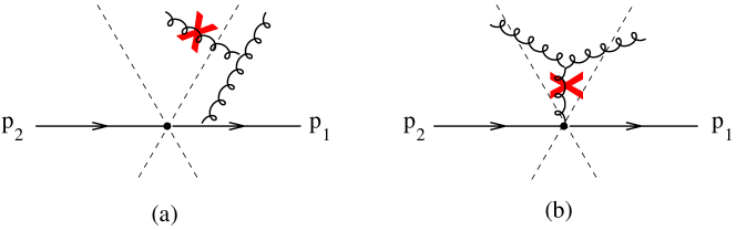
Figure 3: The two representative contributions corresponding to two soft correlated emissions. The red cross corresponds to the constraint $-\Theta(v(k)-v)$ on soft gluon $k$.

The contribution in the last line of eq. (6) corresponds to hard partons outside the slice emitting a soft gluon inside the slice (the terms containing $\mathcal{H}_{3}^{(1)}$), and the corresponding virtual corrections (the term containing $\mathcal{H}_{2}^{(1)}$). This contribution is symbolically represented in Fig. 4.

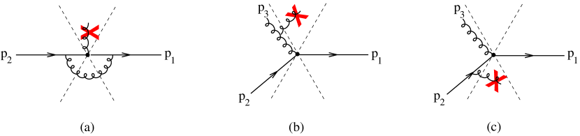
Figure 4: Representative configurations corresponding to a soft gluon emitted from hard $\mathcal{O}(\alpha_{s})$ configurations. The red cross corresponds to the constraint $-\Theta(v(k)-v)$ on soft gluon $k$.

In particular, Fig. 4a represents the term containing $\mathcal{H}_{2}^{(1)}$, and Fig. 4b corresponds to the part of the term containing $\mathcal{H}_{3}^{(1)}$ where soft gluon $k$ is emitted by the two dipoles containing hard gluon $p_{3}$. Finally, Fig. 4c represents the part of the term containing $\mathcal{H}_{3}^{(1)}$ where soft gluon $k$ is emitted by the quark-antiquark dipole.

Comparison with Event2.

We now compare the differential distribution in $v$ obtained from the expansion in eq. (6) to the full QCD result obtained with the program Event2 Catani:1996vz . Specifically, we consider both the transverse energy as well as the energy distribution in the rapidity slice of width $\Delta\eta$ and we plot the quantity

$$\Delta(L)\coloneqq\frac{1}{\sigma_{0}}\left(\frac{d\Sigma^{\rm NLO}}{dL}-\frac{d\Sigma^{\rm EXP.}}{dL}\right)\,,$$ (115)

where $d\Sigma^{\rm NLO}$ is the $\alpha_{s}^{2}/(2\pi)^{2}$ coefficient of the NLO distribution extracted from Event2 and $d\Sigma^{\rm EXP.}$ is the $\alpha_{s}^{2}/(2\pi)^{2}$ coefficient the derivative of Eq. (6). Eq. (115) is shown in Fig. 5 for different values of the parameter $c=\cos\theta_{\rm jet}$. At NLL, one expects

$$\lim_{L\to\infty}\Delta(L)=0\,,$$ (116)

as is clearly confirmed by Fig. 5, which validates our predictions for the next-to-leading non-global corrections, up to ${\cal O}\left(\alpha_{s}^{2}\right)$. In the case of the energy distribution and $c>1/2$, we also compared the result of our calculation to the analytic result of Ref. Becher:2016mmh and found agreement up to ${\cal O}(\alpha_{s}^{2})$ for the values of $\delta$ adopted there.

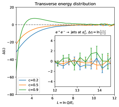
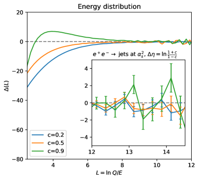
Figure 5: Fixed order tests against Event2 for transverse energy (left) and energy (right) distributions and different widths of the rapidity slice.

7 Conclusions

In this article we have presented a formalism for the resummation of next-to-leading non-global logarithms in QCD. Problems sensitive to non-global logarithms are ubiquitous in collider physics, whenever one considers observables which are sensitive to QCD radiation only in limited angular regions of the phase space. As a case study, we have considered both the transverse energy and energy distribution in a rapidity slice with respect to the thrust axis in $e^{+}e^{-}$ annihilation. We showed that the resummed cumulative cross section (5) can be expressed as a sum of convolutions between hard factors (encoding the contribution of hard radiation) and soft factors (that resum the soft radiative corrections). While the hard factors do not contain large logarithms, the soft factors contain logarithmically enhanced corrections that are resummed by a set of non-linear evolution equations in the large-$N_{c}$ limit. We have computed all ingredients necessary for the resummation of the NLL non-global corrections, namely the hard factors ${\cal H}_{2}$, ${\cal H}_{3}$ up to ${\cal O}\left(\alpha_{s}\right)$ (cf. Eqs. (87), (5)), as well as the evolution kernel for the resummation of the soft factors $S_{2}$, $S_{3}$ up to ${\cal O}\left(\alpha_{s}^{2}\right)$ (cf. Eqs. (31), (4.1)). We used these results to carry out a ${\cal O}(\alpha_{s}^{2})$ fixed-order calculation at finite $N_{c}$ that is in excellent agreement with the full QCD prediction at ${\cal O}(\alpha_{s}^{2})$ for asymptotically small values of the considered observable.

A natural step forward will be the all-order solution of the evolution equations presented here and thus the resummation of NLL non-global corrections with the corresponding study of their phenomenological impact. We envision that the most efficient way to achieve this is by means of Monte Carlo technology. This will be addressed in detail in a forthcoming publication. We finally stress that the formulation derived in this article is not tailored to a specific observable and thus can be applied to other infrared safe observables sensitive to soft radiation emitted away from the large energy flow of the scattering process. In particular, the entire process dependence is encoded in the hard factors while the evolution of the soft factors is universal, which will ultimately allow the resummation of next-to-leading non-global logarithms for hadron collider observables. The precise calculation of these corrections enters the precise description of several collider observables involving jets. An notable example is the fraction of gluon-fusion events in Higgs production in association with two jets with VBF selections cuts Hatta:2020wre , or observables defined by means of jet substructure technology Rubin:2010fc ; Neill:2018yet ; Lifson:2020gua .

The application to observables sensitive to collinear radiation (e.g. the light hemisphere mass in $e^{+}e^{-}$), on the other hand, requires extra care since our formulation does not immediately apply in these cases. One possible way forward would be the calculation of the global corrections using standard resummation technology supplemented by a non-global correction factor obtained by subtracting the global contributions during the numerical integration of the evolution equation derived in this article. This will require a careful extension of the Monte Carlo method of Ref. Dasgupta:2001sh , where this subtraction is carried out at LL accuracy. Another interesting future direction will concern the comparison of our formalism to the formulations of Refs. Caron-Huot:2015bja ; Becher:2016mmh . This can be done by explicitly computing the evolution kernels in Eqs. (31), (4.1) for a specific source corresponding to a given observable. Moreover, from a theoretical point of view it could be interesting to consider the inclusion of subleading-$N_{c}$ corrections to the evolution kernel. Although such corrections have been observed to be usually small in known cases Hatta:2020wre ; Hamilton:2020rcu , their theoretical understanding must be improved in view of high precision phenomenology.

References

- (1) M. Dasgupta and G. P. Salam, Resummation of nonglobal QCD observables, Phys. Lett. B 512 (2001) 323–330, [hep-ph/0104277].
- (2) M. Dasgupta and G. P. Salam, Accounting for coherence in interjet E(t) flow: A Case study, JHEP 03 (2002) 017, [hep-ph/0203009].
- (3) A. Banfi, G. Marchesini and G. Smye, Away from jet energy flow, JHEP 08 (2002) 006, [hep-ph/0206076].
- (4) M. Dasgupta, F. A. Dreyer, K. Hamilton, P. F. Monni and G. P. Salam, Logarithmic accuracy of parton showers: a fixed-order study, JHEP 09 (2018) 033, [1805.09327].
- (5) G. Bewick, S. Ferrario Ravasio, P. Richardson and M. H. Seymour, Logarithmic accuracy of angular-ordered parton showers, JHEP 04 (2020) 019, [1904.11866].
- (6) M. Dasgupta, F. A. Dreyer, K. Hamilton, P. F. Monni, G. P. Salam and G. Soyez, Parton showers beyond leading logarithmic accuracy, Phys. Rev. Lett. 125 (2020) 052002, [2002.11114].
- (7) J. R. Forshaw, J. Holguin and S. Plätzer, Building a consistent parton shower, JHEP 09 (2020) 014, [2003.06400].
- (8) S. Plätzer and I. Ruffa, Towards Colour Flow Evolution at Two Loops, 2012.15215.
- (9) K. Hamilton, R. Medves, G. P. Salam, L. Scyboz and G. Soyez, Colour and logarithmic accuracy in final-state parton showers, 2011.10054.
- (10) Z. Nagy and D. E. Soper, Summations of large logarithms by parton showers, 2011.04773.
- (11) Z. Nagy and D. E. Soper, Summations by parton showers of large logarithms in electron-positron annihilation, 2011.04777.
- (12) A. Karlberg, G. P. Salam, L. Scyboz and R. Verheyen, Spin correlations in final-state parton showers and jet observables, 2103.16526.
- (13) F. Dulat, S. Höche and S. Prestel, Leading-Color Fully Differential Two-Loop Soft Corrections to QCD Dipole Showers, Phys. Rev. D 98 (2018) 074013, [1805.03757].
- (14) H. Weigert, Nonglobal jet evolution at finite N(c), Nucl. Phys. B 685 (2004) 321–350, [hep-ph/0312050].
- (15) Y. Hatta, Relating e+ e- annihilation to high energy scattering at weak and strong coupling, JHEP 11 (2008) 057, [0810.0889].
- (16) S. Caron-Huot, Resummation of non-global logarithms and the BFKL equation, JHEP 03 (2018) 036, [1501.03754].
- (17) J. Forshaw, J. Keates and S. Marzani, Jet vetoing at the LHC, JHEP 07 (2009) 023, [0905.1350].
- (18) R. M. Duran Delgado, J. R. Forshaw, S. Marzani and M. H. Seymour, The dijet cross section with a jet veto, JHEP 08 (2011) 157, [1107.2084].
- (19) M. D. Schwartz and H. X. Zhu, Nonglobal logarithms at three loops, four loops, five loops, and beyond, Phys. Rev. D 90 (2014) 065004, [1403.4949].
- (20) T. Becher, M. Neubert, L. Rothen and D. Y. Shao, Effective Field Theory for Jet Processes, Phys. Rev. Lett. 116 (2016) 192001, [1508.06645].
- (21) A. J. Larkoski, I. Moult and D. Neill, Non-Global Logarithms, Factorization, and the Soft Substructure of Jets, JHEP 09 (2015) 143, [1501.04596].
- (22) T. Becher, M. Neubert, L. Rothen and D. Y. Shao, Factorization and Resummation for Jet Processes, JHEP 11 (2016) 019, [1605.02737].
- (23) T. Becher, B. D. Pecjak and D. Y. Shao, Factorization for the light-jet mass and hemisphere soft function, JHEP 12 (2016) 018, [1610.01608].
- (24) D. Neill, The Asymptotic Form of Non-Global Logarithms, Black Disc Saturation, and Gluonic Deserts, JHEP 01 (2017) 109, [1610.02031].
- (25) S. Caron-Huot and M. Herranen, High-energy evolution to three loops, JHEP 02 (2018) 058, [1604.07417].
- (26) A. J. Larkoski, I. Moult and D. Neill, The Analytic Structure of Non-Global Logarithms: Convergence of the Dressed Gluon Expansion, JHEP 11 (2016) 089, [1609.04011].
- (27) T. Becher, R. Rahn and D. Y. Shao, Non-global and rapidity logarithms in narrow jet broadening, JHEP 10 (2017) 030, [1708.04516].
- (28) R. Ángeles Martínez, M. De Angelis, J. R. Forshaw, S. Plätzer and M. H. Seymour, Soft gluon evolution and non-global logarithms, JHEP 05 (2018) 044, [1802.08531].
- (29) M. Balsiger, T. Becher and D. Y. Shao, Non-global logarithms in jet and isolation cone cross sections, JHEP 08 (2018) 104, [1803.07045].
- (30) D. Neill, Non-Global and Clustering Effects for Groomed Multi-Prong Jet Shapes, JHEP 02 (2019) 114, [1808.04897].
- (31) M. Balsiger, T. Becher and D. Y. Shao, NLL′ resummation of jet mass, JHEP 04 (2019) 020, [1901.09038].
- (32) M. Balsiger, T. Becher and A. Ferroglia, Resummation of non-global logarithms in cross sections with massive particles, JHEP 09 (2020) 029, [2006.00014].
- (33) Y. Hatta and T. Ueda, Resummation of non-global logarithms at finite , Nucl. Phys. B 874 (2013) 808–820, [1304.6930].
- (34) Y. Hagiwara, Y. Hatta and T. Ueda, Hemisphere jet mass distribution at finite , Phys. Lett. B 756 (2016) 254–258, [1507.07641].
- (35) Y. Hatta and T. Ueda, Non-global logarithms in hadron collisions at = 3, Nucl. Phys. B 962 (2021) 115273, [2011.04154].
- (36) J. R. Forshaw, A. Kyrieleis and M. H. Seymour, Super-leading logarithms in non-global observables in QCD, JHEP 08 (2006) 059, [hep-ph/0604094].
- (37) J. R. Forshaw, A. Kyrieleis and M. H. Seymour, Super-leading logarithms in non-global observables in QCD: Colour basis independent calculation, JHEP 09 (2008) 128, [0808.1269].
- (38) S. Catani and M. H. Seymour, A General algorithm for calculating jet cross-sections in NLO QCD, Nucl. Phys. B 485 (1997) 291–419, [hep-ph/9605323].
- (39) A. Bassetto, M. Ciafaloni and G. Marchesini, Jet Structure and Infrared Sensitive Quantities in Perturbative QCD, Phys. Rept. 100 (1983) 201–272.
- (40) F. Fiorani, G. Marchesini and L. Reina, Soft Gluon Factorization and Multi - Gluon Amplitude, Nucl. Phys. B 309 (1988) 439–460.
- (41) S. Catani, L. Trentadue, G. Turnock and B. R. Webber, Resummation of large logarithms in e+ e- event shape distributions, Nucl. Phys. B 407 (1993) 3–42.
- (42) M. Dasgupta, F. Dreyer, G. P. Salam and G. Soyez, Small-radius jets to all orders in QCD, JHEP 04 (2015) 039, [1411.5182].
- (43) L. Magnea, Analytic resummation for the quark form-factor in QCD, Nucl. Phys. B 593 (2001) 269–288, [hep-ph/0006255].
- (44) J. M. Campbell and E. W. N. Glover, Double unresolved approximations to multiparton scattering amplitudes, Nucl. Phys. B 527 (1998) 264–288, [hep-ph/9710255].
- (45) A. Gehrmann-De Ridder, T. Gehrmann and E. Glover, Antenna subtraction at NNLO, JHEP 09 (2005) 056, [hep-ph/0505111].
- (46) E. Gardi and L. Magnea, Factorization constraints for soft anomalous dimensions in QCD scattering amplitudes, JHEP 03 (2009) 079, [0901.1091].
- (47) S. Catani and M. Grazzini, The soft gluon current at one loop order, Nucl. Phys. B 591 (2000) 435–454, [hep-ph/0007142].
- (48) R. Ángeles Martínez, J. R. Forshaw and M. H. Seymour, Ordering multiple soft gluon emissions, Phys. Rev. Lett. 116 (2016) 212003, [1602.00623].
- (49) A. Banfi, H. McAslan, P. F. Monni and G. Zanderighi, A general method for the resummation of event-shape distributions in annihilation, JHEP 05 (2015) 102, [1412.2126].
- (50) A. Banfi, B. K. El-Menoufi and P. F. Monni, The Sudakov radiator for jet observables and the soft physical coupling, JHEP 01 (2019) 083, [1807.11487].
- (51) C. W. Bauer and P. F. Monni, A formalism for the resummation of non-factorizable observables in SCET, JHEP 05 (2020) 005, [1906.11258].
- (52) Y. L. Dokshitzer, A. Lucenti, G. Marchesini and G. P. Salam, Universality of 1/Q corrections to jet-shape observables rescued, Nucl. Phys. B 511 (1998) 396–418, [hep-ph/9707532].
- (53) E. Laenen, G. F. Sterman and W. Vogelsang, Recoil and threshold corrections in short distance cross-sections, Phys. Rev. D 63 (2001) 114018, [hep-ph/0010080].
- (54) L. J. Dixon, L. Magnea and G. F. Sterman, Universal structure of subleading infrared poles in gauge theory amplitudes, JHEP 08 (2008) 022, [0805.3515].
- (55) M. Rubin, Non-Global Logarithms in Filtered Jet Algorithms, JHEP 05 (2010) 005, [1002.4557].
- (56) A. Lifson, G. P. Salam and G. Soyez, Calculating the primary Lund Jet Plane density, JHEP 10 (2020) 170, [2007.06578].