Neuro-Symbolic VQA: A review from the perspective of AGI desiderata
Ian Berlot-Attwell
An ultimate goal of the AI and ML fields is artificial general intelligence (AGI); although such systems remain science fiction, various models exhibit aspects of AGI. In this work, we look at neuro-symbolic (NS) approaches to visual question answering (VQA) from the perspective of AGI desiderata. We see how well these systems meet these desiderata, and how the desiderata often pull the scientist in opposing directions. It is my hope that through this work we can temper model evaluation on benchmarks with a discussion of the properties of these systems and their potential for future extension.
1 Introduction
VQA is the task of answering a natural language question about a given image. NS approaches combine neural networks with a symbolic component (e.g., symbolic reasoning, symbolic representations, or exploiting pre-existing symbolic knowledge). NS approaches to VQA are of particular interest as they may promote compositional generalization [31, 4, 10] (i.e., the ability to understand new combinations of previously acquired concepts; for instance, \sayBuzz Aldrin wielded a glass hammer). NS approaches also promise to be more interpretable [19, 23], and may allow for simpler skill transfer between tasks.
Of the AGI desiderata identified by Bieger et al. [17], we discuss: natural growth (the ability to continue learning without human re-design), traceability (the ability to give step-by-step explanations of decisions, even if step execution cannot be explained), transfer-learning (the ability to exploit previous knowledge when learning new knowledge), few-shot learning, and self-awareness of limitations. For few-shot learning, we mostly consider compositional generalization (the ability to understand previously learned concepts in new combinations). These desiderata were chosen as they can be found in neuro-symbolic VQA models. As these desiderata are meaningless if we do not take practical considerations into account, we also discuss performance, scalability, and training data when they become particularly relevant.
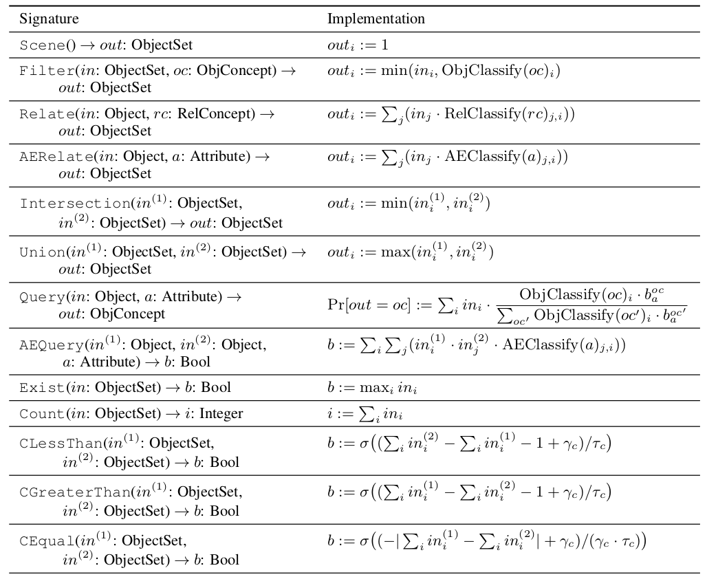
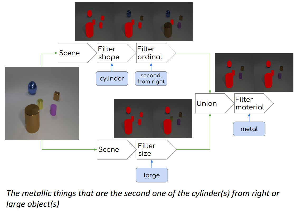
In this work: Attribute refers to properties of an object (e.g., colour, or shape), Concept refers to possible values of an Attribute (e.g., red, or circle), and Relations are possible relations between two or more objects (e.g., besides, under, or is wearing). A Domain Specific Language (DSL) is a symbolic language that can be used to represent any question in the domain. For instance, the DSL {sphere, cube, left_of()} can represent Is there a cube left of a sphere? as left_of(cube, sphere). We call the representation of a question in a given DSL, the Program.
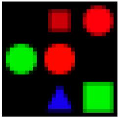
Some frequently used datasets are: the VQA 1.0 dataset [5] of natural images with human-created questions (see Fig 4), the synthetic SHAPES dataset [4] of shapes on a grid with compositional questions (see Fig 2, 5), the CLEVR dataset [14] which is similar to SHAPES but using 3D figures (see Fig 6), and the GQA dataset [27] of natural images with synthetic compositional questions (see Fig 7). A variant of CLEVR, CLEVR-CoGenT [14], is also used to test compositional generalization; in this dataset, cubes and cylinders are different colours and swap colour palettes between train and test time.
2 Module Networks
In the module network approach, the model learns a set of small networks (i.e., modules) and assembles them based on the question [4]. The modules are described by a DSL, which specifies the arity and input/output types of the modules that the network has.
2.1 NMN Architecture
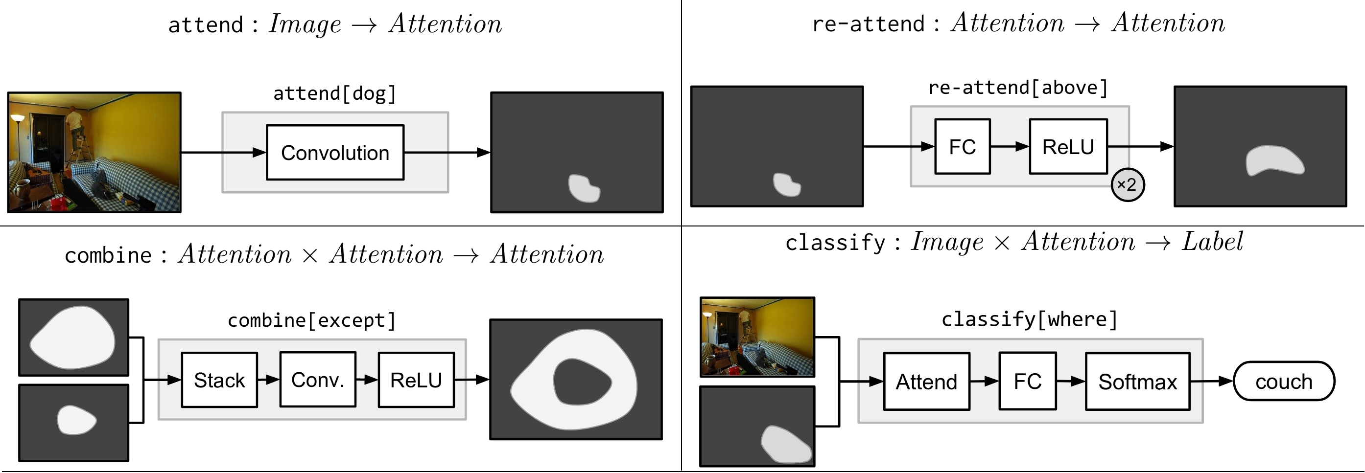
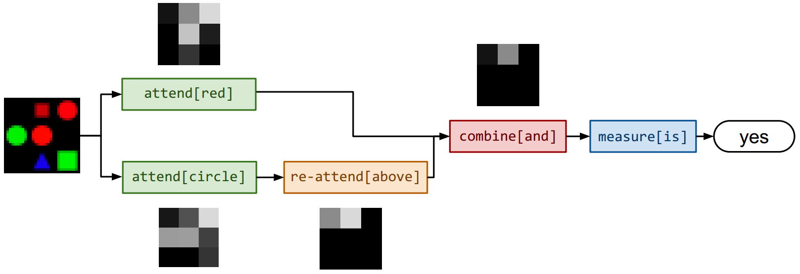
The Neural Module Network (NMN) [4] was the first module network for VQA. The NMN DSL lists 5 modules types (e.g., attend), each with distinct architectures (see Fig 1). Most modules create or modify heatmaps of the image. Each module type has a unique instance per specific task. The sample execution in Fig 2 shows two such instances: attend[circle] and attend[red]. To produce the program, the NMN lemmatizes the question, applies the Stanford dependency parser [2], and applies fixed rules.
To overcome the limitations of the program generator and to incorporate a linguistic prior into the responses, the architecture above is ensembled with a blind LSTM model (i.e., predicts the answer based on the question alone). Specifically, the weighted geometric mean of the distributions is calculated; weights are determined by the text and image features. The system is trained end-to-end [4].
2.2 NMN: Strengths & Weaknesses
The natural growth of this architecture is critically limited by the immutable rules-based parser. The authors note that the parser has problems; it aggressively simplifies the question (e.g., replacing plural nouns with singular nouns), and it introduces spurious predicates in roughly 10-20% of VQA 1.0 questions (e.g., parsing \sayare these people most likely experiencing a work day? as be(people, likely)). However, they perform no tests with ground-truth programs, even though SHAPES has ground-truth programs.
In principle, the traceability is good as the program is a trace, but there are caveats (see Section 2.6). Transfer learning to another task by re-using modules is promising but untested. As each concept has its own independent module weights, the model cannot internally transfer acquired knowledge (e.g., learning find[wolf] using find[dog]), or exploit prior linguistic knowledge (e.g., via GloVe [3] or BERT [26] embeddings).
The NMN exhibits compositional generalization through new combinations of the learned modules. Andreas et al. [4] tested the model’s ability with the SHAPES dataset. However, although SHAPES tests complex compositional questions, all shapes are of the same size and aligned on a grid (see Fig 5). This compensates for one of NMN’s flaws, that reasoning steps, such as \saylook at the shape to the left, are executed by a fixed re-attend[left] module without access to the input question or image, only the previous modules’ outputs. Using a fixed grid simplifies this, e.g., attend[above] need not concern itself with objects that are above and of a different size, or occluded. The authors demonstrate that the model can generalize to SHAPES questions who’s programs are one more module longer than seen at train time, but do not try combinations of subtasks that are new at test time (we discuss further in Section 2.5).
The NMN [4] has no limitation awareness; in fact, a common failure mode was to return a plausible response that is disconnected from the image. Although the NMN has no explicit confidence in its response, it indicates relative confidence between the module network and LSTM via the weights used in the ensemble. The model achieved SOTA performance on VQA 1.0 at the time of publication ( accuracy). Although we now know that the dataset suffers from strong language priors [9, 11], these priors were addressed through a blind baseline.
2.3 N2NMN: Improving the NMN
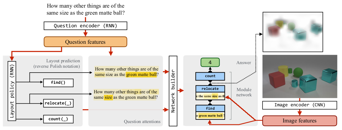
The End-to-End Module Network (N2NMN) [13] followed the NMN. Primarily, it removed the blind model and produced programs (in reverse Polish notation) with a seq2seq encoder-decoder LSTM architecture. Additionally, each module type (e.g., attend) has exactly one instance and is provided a text-context vector, , (an attention over input tokens), and image features, , (extracted by VGG-16 [6]). The modules and their architectures are in Fig 3, and Fig 10 illustrates model execution.
Evaluation of the N2NMN on VQA 1.0 and SHAPES demonstrates increased performance over NMN. However, end-to-end training of the program generator through the modules via backpropagation is impossible. Executing the N2NMN requires arranging the modules; thus we must sample a discrete program from the program parser, and we cannot backpropagate through the sampling operation. REINFORCE can be used but causes a drop in performance ( on SHAPES and on CLEVR). Instead, the N2NMN is trained in two stages: initially the generator is encouraged to mimic a provided expert parser, afterwards it is fine-tuned with REINFORCE. Thus training requires an expert parser to mimic.
2.4 N2NMN: Strengths & Weaknesses
As the N2NMN’s [13] parser is trained on examples instead of being rule-based, the N2NMN improves on the natural growth of the NMN. However, the N2NMN modules are still low-capacity, with architectures designed for the modules’ intended role – some modules such as and and or have no learnable parameters (see Fig 3). Unless we violate compositionality by using multiple modules to implement a single operation, then each operation’s capacity is severely limited.
The vector passed to each module improves within-task transfer learning, as each operation has a single module. Thus, for example, the find module can learn to find wolves based on its knowledge of dogs. However, complicates transfer learning to a different task; we require a mechanism to provide . also reduces traceability, as the program is coarser, and the user must interpret the attention defining to guess what each module does. Furthermore, Subramanian et al. [33] suggest that using may damage compositional generalization and traceability, as it can leak information, causing hybrid operations. For instance, \sayred objects left of the cube may correspond to filter[red](relate[left](find[cube])). However, through , relate[left] may learn to find objects that are to the left and red. This damages compositionality (as relate will not behave as it should), and traceability (as the name relate becomes misleading if relate also does filtering); possible solutions, such as supervising intermediary modules outputs, are discussed in Section 2.6.
The compositionality is tested by evaluation on CLEVR and SHAPES, however the authors do not test scenarios where the question distribution varies between train and test time. Other minor methodological flaws are that Hu et al. [13] omitted the performance when training without program supervision on VQA 1.0, and they augmented CLEVR image features with two channels for position data, without an ablation test. Like the NMN, the N2NMN has no limitation awareness.
2.5 Compositional Generalization and Few-Shot Learning in Module Networks
Underpinning module networks is the idea that we can solve new combinations of concepts with new combinations of modules. We can test this assertion through CLOSURE [24], a dataset for testing the compositional generalization of models trained on CLEVR. Where CLEVR’s test questions are generated from one of 90 templates seen at train time [14], CLOSURE is generated from five new templates created by replacing spatial comparisons with attribute comparisons.
The authors used CLOSURE to test the compositional generalization of various SOTA models, and the effectiveness of few-shot learning. Critically, the NMN-type model tested (dubbed Tensor-NMN [15]) failed to generalize, even with ground-truth programs. The Tensor-NMN architecture’s modules take and return tensors of fixed dimensions; all modules are residual blocks of two convolutions, with higher arity modules first merging input channels with convolution. A program parser similar to the N2NMN’s is used. The Tensor-NMN DSL is similar to NMN’s, with multiple types that have different instantiations (e.g., filter_colour[blue], filter_colour[red], etc…). This demonstrates that the N2NMN parser is problematic, and that the N2NMN and NMN modules may not function as intended when rearranged.
The authors speculated that reducing the dimensionality of the intermediary features would improve generalization. They thus developed Vector-NMN, which only passes vectors between modules. Vector-NMN uses the same program parser as Tensor-NMN and a different module architecture. All modules are two consecutive FiLM [20] blocks applied to ResNet101 features of the input image, followed by max-pooling to reduce them to a vector. The FiLM blocks contain convolutional filters shared among all modules, which are modulated with additive and multiplicative weights produced by a MLP. This MLP processes the vector outputs of any previous modules along with a learned module-embedding representing the module’s role. Bahdanau et al.[24] found that Vector-NMN had near perfect generalization to CLOSURE when given the ground-truth programs, with the exception of one family of questions. Here, Vector-NMN still outperformed Tensor-NMN. However, we cannot conclude that dimensionality alone determines generalization; the authors overlook key differences between the models. Notably: Vector-NMN uses weight sharing, is architecturally more similar to FiLM than Tensor-NMN, and its modules get image features as an argument. Comparison with other models using lower dimensional intermediary values such as TbD [19] (mostly matrices) and Visual-NMN [33] (vectors) would help with the confounding variables.
Although self-evident, the largest limitation of CLOSURE is that it is a necessary, but insufficient, condition for compositional generalization on CLEVR. For instance, all CLOSURE questions contain the same number of referring expressions as some CLEVR question. Consequently, CLOSURE only tests compositional generalization on questions that are at most as complex as CLEVR questions.
The authors also test few-shot learning by training Vector-NMN on 36 questions from each CLOSURE template without program annotations. The findings were that in six of the seven families the model performed well after training, demonstrating that the seq2seq LSTM program-parser can exhibit few-shot learning using REINFORCE only. However, fine-tuning failed on the seventh family; the authors concluded that it was because REINFORCE was not sampling good programs. This suggests that there may be scalability issues as more complex DSLs are used.
2.6 Fidelity in Module Networks
Failure to generalize with ground truth programs calls into question the faithfulness of modules’ behaviour to the program DSL, and thus the traceability. Liu et al. [29] found that Tensor-NMN modified for image segmentation exhibited good fidelity, and that the shared tensor output dimensions of all modules facilitated transfer-learning (see Fig 11). Specifically, they could apply the last module, which produces the output segmentation heatmap, to any intermediate module, thus producing an intermediate image segmentation. The modules’ fidelity was not perfect; one module ultimately functioned as a preprocessing step instead of the desired behaviour. Similarly, Subramanian et al. [33] found poor fidelity in a module network using probabilistic sets as intermediary values. They found that restricting module architectures or supervising module outputs improved fidelity; this creates a tradeoff between improving traceability through fidelity, and reducing natural growth due to lower capacity modules, or training requiring additional annotations.
3 Addressing the Problems of Discrete Programs
3.1 Reducing model capacity
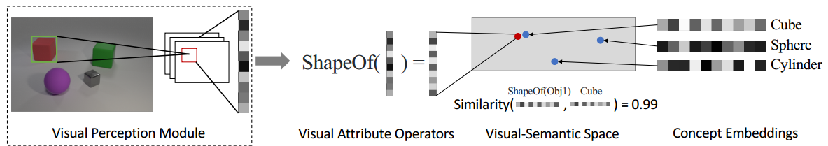
The Neuro-Symbolic Concept Learner (NS-CL) resolves the module composition and fidelity issues by using fixed implementations for most elements of the DSL (see Fig 9). This ensures perfect traceability, and some limitation awareness to the model; ambiguous or invalid questions cause the execution engine to throw an error. However, this comes at the cost natural growth; the DSL’s execution is fixed.
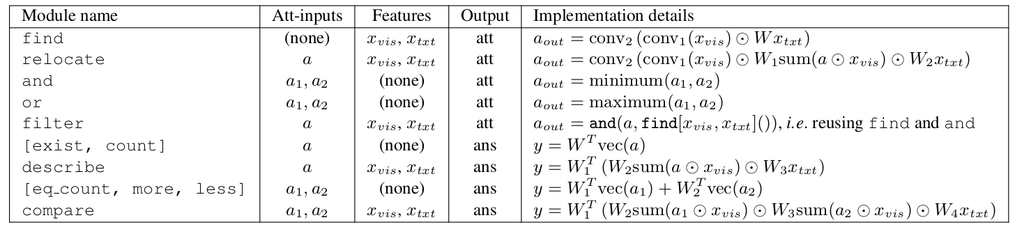
Instead of processing attention maps, the NS-CL [30] identifies objects with a pre-trained Mask R-CNN [12] and processes probabilistic sets of objects. Each object has a vector representation of ResNet-34 features. The execution engine’s learned components are: i) networks for projecting an object’s feature vector into an attribute space, and ii) a vector in said attribute space for each concept specified by the user (see Fig 8). This structured representation allows for some transfer learning to other tasks. The authors demonstrated this by freezing the attribute embedding networks and using them with a different DSL for CLEVR image retrieval.
The parser architecture is also changed, and a rule-based preprocessing step is added. Concepts & attributes in the question are replaced with placeholders, thus allowing new attributes to be recognized by updating the list of attributes. This combined with the disentangled attribute representations facilitates few-shot learning; Mao et al. [30] show that when learning a new colour from example images, the NS-CL has a test accuracy of 93.9%, outperforming TbD [19] and Tensor-NMN by and respectively. Furthermore, if attribute detection could be automated, then this would facilitate natural growth to learn new attributes and concepts. The authors do not report a seq2seq baseline.
Like module networks, the design promises compositional generalization. The authors test on CLEVR and CLEVR-CoGenT, demonstrating the NS-CL is capable of answering compositional questions and exhibits compositional generalization under a change of attribute combinations. The authors claim that NS-CL can generalize to new questions, and support this by training and testing on a split of CLEVR based on program depth. This implicitly splits by CLEVR question template, and is thus similar to CLOSURE.
On a practical note, the additional structure improves performance on CLEVR compared to the SOTA module network approaches such as TbD [19]. Furthermore, the NS-CL does not require program annotations at train time and is more data-efficient than TbD. Curriculum learning is used to train the model, and an ablation demonstrated that removing curriculum learning resulted in either non-convergent training, or performance on-par with random guessing [30]. The first stage of training consists of short questions about attributes, the second stage adds short relational questions, and the third stage adds all remaining questions. During the first two stages, REINFORCE is used to train the program parser. In stage three, the exact REINFORCE gradient is calculated by finding , the set of programs returning the correct response. The attribute embedding networks and concept vectors are trained simultaneously through backpropagation, although they are initially frozen in stage 3. However, finding the true is intractable. After writing to the authors, I determined that they restricted their search to programs from templates extracted from ground-truth programs. This indicates that scalability with DSL complexity is problematic, and the severity is unclear as the authors do not report performance when using normal REINFORCE in stage 3.
3.2 Continuous Programs
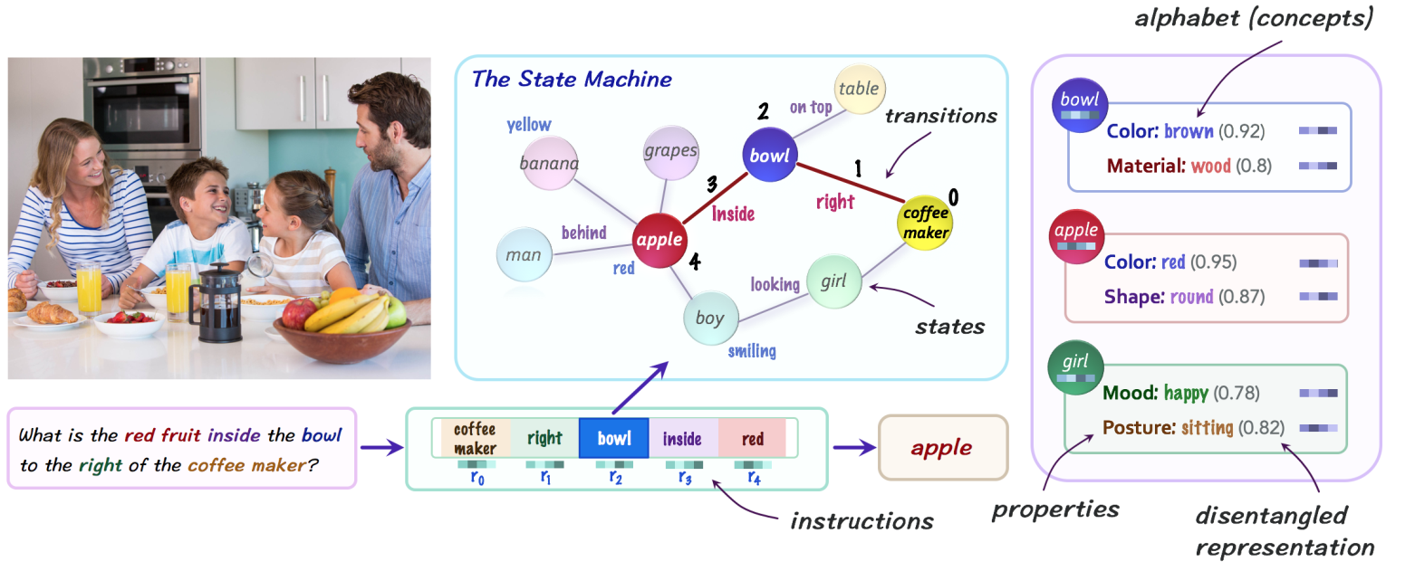
Where the NS-CL addresses the issues arising from discrete programs with a (mostly) fixed execution engine, the Neural State Machine (NSM) instead resolves these issues by using continuous programs. Although it doesn’t use a DSL, the NSM still incorporates prior knowledge in the form of the object-types, concepts, attributes, and binary relationships that can occur in an image. Specifically, NSM performs soft reasoning over a graph representation of the image (see Fig 13). This design hurts traceability, as the reasoning steps are now vectors. At best, the meaning of these reasoning instructions can be guessed based on the attention over the question tokens that created them.
To create this graph representation, the NSM requires: the set of object-types, the attributes, a set of concepts for each attribute, and the set of binary relationships. First, a node is created in the graph for each object detected by a Mask R-CNN. This Mask R-CNN also produces distributions over object type and attributes; this requires scene graphs at train time. Next, for all objects that are sufficiently close in the image a directed edge is created in each direction between the corresponding nodes. A graph attention network [21] then produces a distribution over binary relationships for each edge. Each distribution is summarized as a weighted average over learned concept/object/relationship embeddings, initialized with GloVe. This graph is the final representation of the image that the NSM reasons over. The NSM redistributes attention over the nodes based on the reasoning instruction, sometimes through edges.
This design severely limits the natural growth of the model compared to the approaches seen thus far. Previously, another attribute or concept could be added by the addition of a module (e.g., NMN), or the updating of a list (e.g., NS-CL); for the NSM this requires changing the model’s architecture to alter the arity of various networks. However, the discrete scene graph representation does allow for the NSM to be cleanly divided into two components that can be reused in other tasks, potentially allowing for transfer learning, albeit in a manner that is coarser than module reuse in a module network. The fixed edge creation heuristic is also problematic as the model cannot reason about long-distance relationships (e.g., between a thrower and catcher on a game field).
The flow of attention through the graph is controlled by reasoning instructions that are generated from the question, somewhat analogous to the N2NMN’s vectors. The reasoning instructions are weighted averages of vectors representing the input tokens of the question, and are produced by an encoder-decoder model. However, where the N2NMN learns token embeddings, the NSM represents each token as a weighted average between the GloVe embedding and the learned object, concept, and relationship embeddings. Ablation indicates that representing both the question and image as weighted averages of the same embeddings improves performance. Furthermore, the NSM always decodes a fixed number of reasoning instructions, thus allowing the parser to be trained through backpropagation.
Starting from uniform attention over nodes, the NSM sequentially updates the attention based on each reasoning instruction. The update is a linear combination of two mechanisms; one assigns attention based on attributes and object-type, the other shifts attention along edges based on binary relation. Final classification is done by a 2-layer MLP given the encoded question (from the encoder-decoder reasoning instruction parser), and a vector representation of the graph. The graph representation is produced by first averaging each node’s attribute vectors based on the last reasoning instruction, and then averaging these vectors based on the final attention over nodes.
The authors demonstrate the NSM’s compositional generalization through splits of GQA where object types are removed at train time and introduced at test time. Note that object detector is trained on all objects. However, GQA questions are generated from templates, and the authors do not have a CLOSURE-like test for generalization to new question structures.
4 Achieving Desiderata via Regularization
The previous models incorporated prior symbolic knowledge directly into their reasoning processes; an alternative approach is to instead leverage this knowledge in model optimization. Xie et al. [32] defines a regularizer, , that encodes propositional logic describing the domain (e.g., wear(person,hat) exists(person) exists(hat)). Note that unlike the previously discussed models, the authors tested on the related task of visual relationship prediction (VRP): given an image, the bounding boxes of two objects, and their respective object-type, VRP seeks the relationship between the objects.
The regularizer uses a trained Logic Embedding Network with Semantic Regularization (LENSR). To train a VRP model, , the first step is to train LENSR, , on the given rules, and then freeze the LENSR weights. LENSR is a modified graph convolutional network [16] that encodes propositional logic formulas as a vector. To encourage the encoding of assignments to be closer to formulas that they satisfy, LENSR is trained with a regularized triplet loss (details in Appendix 6.4). is then trained with cross entropy loss regularized with . is the formula of rules (in d-DNNF form) that apply to this batch of training examples, and is the weighted average of the LENSR embeddings of all possible solutions for the th example in the batch, weighted by (see Fig 14).
LENSR demonstrates an approach for transfer learning by which pre-existing symbolic knowledge guides training. Systems that automatically extract symbolic knowledge from text, such as COMET [25], may thus allow natural growth from unstructured data. However, there are limitations. LENSR encodes propositions by summing the GloVe embeddings of their components (e.g., on(sphere, block) block+on+sphere), thus loosing order information. Furthermore, LENSR may not scale well as compiling the rules into d-DNNF form is an NP-Hard task.
As to practical considerations, the authors demonstrated that the regularization increases model performance on VRP when is a two-layer MLP, and that their logic loss outperforms semantic loss [22]; they speculate this due to the more complex constraints. They also compare with a TreeLSTM encoder, however previous work using TreeLSTM for logical entailment was under different conditions (see Appendix 6.5).
5 Discussion and Conclusions
In this work, we discuss how various neuro-symbolic VQA models meet a set of AGI desiderata. We find that, in principle, module networks satisfy all the desiderata except for limitation awareness. However, transfer to significantly different tasks is untested, and traceability is closely tied to program fidelity, as is compositionality. Yet, approaches that encourage program fidelity, such as parameter-free modules, often harm natural growth – with the extreme example being the NS-CL. Furthermore, CLOSURE indicates that encoder-decoder program parsers do not exhibit compositional generalization to new combinations of sub-tasks. The NSM avoids the program parser generalization and program supervision problems and achieves the best GQA performance, but at the cost concessions on traceability, transfer learning and natural growth. LENSR suggests that the choice of training procedure may be able to encourage AGI desiderata.
If we seek to overcome the limitations of module networks, then we may be able to improve parser generalization through the training procedure. In addition to NS-CL style curriculum learning, we may be able to apply techniques from domain-generalization by framing families of questions from specific templates as domains. A significant open question about a module network’s natural growth is whether the DSL can be learned from data; it’s possible that a more structured intermediary representation like the NSM may simplify this task – although it may be a lateral move, placing the onus of growth on the scene graph.
Overall, the existence of models exhibiting subsets of the desiderata, combined with the nice interpretation of many of the desiderata in VQA (compositionality as new combinations of old ideas, natural growth as adaption to new questions and domains, traceability as the production of accurate traces, transfer learning within-task as exploiting old knowledge to learn new concepts, and out of task in the usual sense, and self awareness of limitations as identifying invalid questions, or indicating confidence), indicates that VQA may be a rich task for the purposes of developing models that exhibit all of these desiderata. Such work will not bring us AGI, but can provide a clearer image of the challenges that lie on the road there.
6 Appendix
6.1 Sample Questions from VQA Datasets


6.2 DSLs
6.3 Sample Execution


6.4 LENSR Details
The LENSR logic loss is dependent on encoding prepositional logic expressions as vectors [32]. The first step is to convert the expression into d-DNNF form. This form is attractive as it allows for clausal entailment, model counting, model enumeration, model minimization based on cardinality, and probabilistic equivalence testing to be solvable in time polynomial with the size of the d-DNNF formula [1]. Note that as a consequence, conversion from CNF to d-DNNF is NP-Hard [1]. d-DNNF form is both deterministic (the arguments of any disjunction, , are mutually inconsistent) and decomposable (the arguments of any conjunction, , are over disjoint sets of variables) [1].
Once the formula is in d-DNNF form, it is encoded into a vector by LENSR. LENSR is a modified graph convolutional network (GCN) [16]. Before processing by LENSR, the d-DNNF formula is converted into a non-binary expression tree (see in Fig 14), the edges are made undirected, and a “global” node is created that connects to all other nodes. This graph is then processed by the LENSR, and the final LENSR embedding of the global node is used as the final embedding of the formula.
Where a standard GCN shares the same weight matrix across all nodes, LENSR is modified to use heterogeneous node embedding. In other words, there is a distinct weight matrix used for nodes, nodes, leaf nodes, and the global node. To train LENSR, the loss function is used, where is a hyperparameter, is a d-DNNF formula in the training data, is a non-satisfying assignment (expressed as the conjunction of literals for all variables in ) and is a satisfying assignment. For example, we could have , , and . The term is a triplet loss encouraging satisfying assignments to be closer to the formula than non-satisfying assignments. Specifically, where the margin, , is a hyperparameter, and is the LENSR network. The other term () is the semantic regularization component, which encourages properties in the latent space analogous to properties of the d-DNNF. At a high-level, the embeddings of the children of an node should add to (as an analogue to mutual exclusivity), and the embeddings of the children of an node should be orthogonal (as an analogue to operating on disjoint sets of variables). Specifically, , where is the set of nodes, is the set of nodes, is the set of children nodes of in the directed expression tree, and s.t. and , .
Note that the graph convolutional network requires initial embeddings for all nodes. Non-leaf nodes are given an initial embedding based on their type (, , or global), which is shared among all nodes of the same type. The initial embeddings for leaf-nodes are created by taking the sum of the GloVe embeddings of the words comprising the proposition. For example, the proposition wear(person,glasses) is represented as the sum of the GloVe embeddings for \saywear, \sayperson, and \sayglasses.
6.5 LENSR Methodological Flaw
Xie et al. [32] test their model on the VRD dataset [8], and compare against TreeLSTM [7] encoding. They state that TreeLSTM [7] is state-of-the-art. However, to the best of my knowledge, TreeLSTM has never been used on VRD before. Furthermore, the paper they cite concerns encoding natural language rather than logic. Reviewing the references, I found a paper (not cited within the body) demonstrating that for the task of logical entailment, TreeLSTM was the best performing encoding-type model [18]. From this, I assume that authors intended to convey that TreeLSTM was SOTA for determining entailment using embeddings. However, Evans et al. [18] used a modified variant of TreeLSTM where parameters at each node are determined by the corresponding logical operators, and it is unclear whether Xie et al. [32] used the modified or unmodified TreeLSTM. Furthermore, the cited paper used a MLP to determine entailment based on the encodings, as opposed to squared euclidean distance used with the LENSR embeddings. It is unclear how the LENSR authors used the TreeLSTM embeddings, which may make their comparison unfair.
References
- [1] Adnan Darwiche “New Advances in Compiling CNF to Decomposable Negation Normal Form” In IN ECAI, 2004, pp. 328–332
- [2] Marie-Catherine Marneffe and Christopher D. Manning “The Stanford Typed Dependencies Representation” In Coling 2008: Proceedings of the Workshop on Cross-Framework and Cross-Domain Parser Evaluation, CrossParser ’08 Manchester, United Kingdom: Association for Computational Linguistics, 2008, pp. 1–8 URL: https://dl.acm.org/doi/10.5555/1608858.1608859
- [3] Jeffrey Pennington, Richard Socher and Christopher D. Manning “GloVe: Global Vectors for Word Representation” In Empirical Methods in Natural Language Processing (EMNLP), 2014, pp. 1532–1543 URL: http://www.aclweb.org/anthology/D14-1162
- [4] Jacob Andreas, Marcus Rohrbach, Trevor Darrell and Dan Klein “Neural Module Networks”, 2015 arXiv:1511.02799 [cs.CV]
- [5] Stanislaw Antol et al. “VQA: Visual Question Answering” In International Conference on Computer Vision (ICCV), 2015
- [6] Karen Simonyan and Andrew Zisserman “Very Deep Convolutional Networks for Large-Scale Image Recognition” In 3rd International Conference on Learning Representations, ICLR 2015, San Diego, CA, USA, May 7-9, 2015, Conference Track Proceedings, 2015 URL: http://arxiv.org/abs/1409.1556
- [7] Kai Sheng Tai, Richard Socher and Christopher D. Manning “Improved Semantic Representations From Tree-Structured Long Short-Term Memory Networks” In Proceedings of the 53rd Annual Meeting of the Association for Computational Linguistics and the 7th International Joint Conference on Natural Language Processing (Volume 1: Long Papers) Beijing, China: Association for Computational Linguistics, 2015, pp. 1556–1566 DOI: 10.3115/v1/P15-1150
- [8] Cewu Lu, Ranjay Krishna, Michael Bernstein and Li Fei-Fei “Visual Relationship Detection with Language Priors” In European Conference on Computer Vision, 2016 URL: https://cs.stanford.edu/people/ranjaykrishna/vrd/
- [9] Peng Zhang et al. “Yin and Yang: Balancing and Answering Binary Visual Questions” In Conference on Computer Vision and Pattern Recognition (CVPR), 2016
- [10] Tarek R. Besold et al. “Neural-Symbolic Learning and Reasoning: A Survey and Interpretation” In CoRR abs/1711.03902, 2017 arXiv: http://arxiv.org/abs/1711.03902
- [11] Yash Goyal et al. “Making the V in VQA Matter: Elevating the Role of Image Understanding in Visual Question Answering” In Conference on Computer Vision and Pattern Recognition (CVPR), 2017
- [12] K. He, G. Gkioxari, P. Dollár and R. Girshick “Mask R-CNN” In 2017 IEEE International Conference on Computer Vision (ICCV), 2017, pp. 2980–2988
- [13] Ronghang Hu et al. “Learning to Reason: End-To-End Module Networks for Visual Question Answering” In Proceedings of the IEEE International Conference on Computer Vision (ICCV), 2017
- [14] Justin Johnson et al. “CLEVR: A Diagnostic Dataset for Compositional Language and Elementary Visual Reasoning” In CVPR, 2017
- [15] Justin Johnson et al. “Inferring and Executing Programs for Visual Reasoning” In ICCV, 2017
- [16] Thomas N. Kipf and Max Welling “Semi-Supervised Classification with Graph Convolutional Networks” In 5th International Conference on Learning Representations, ICLR 2017, Toulon, France, April 24-26, 2017, Conference Track Proceedings OpenReview.net, 2017 URL: https://openreview.net/forum?id=SJU4ayYgl
- [17] Jordi Bieger and Kristinn Thórisson “Requirements for General Intelligence: A Case Study in Trustworthy Cumulative Learning for Air Traffic Control” In Proceedings of the 1st International FAIM Workshop on Architectures and Evaluation for Generality, Autonomy & Progress in AI (AEGAP 2018), 2018
- [18] Richard Evans et al. “Can Neural Networks Understand Logical Entailment?” In International Conference on Learning Representations, 2018 URL: https://openreview.net/forum?id=SkZxCk-0Z
- [19] David Mascharka, Philip Tran, Ryan Soklaski and Arjun Majumdar “Transparency by Design: Closing the Gap Between Performance and Interpretability in Visual Reasoning” In Proceedings of the IEEE Conference on Computer Vision and Pattern Recognition (CVPR), 2018 URL: https://openaccess.thecvf.com/content_cvpr_2018/html/Mascharka_Transparency_by_Design_CVPR_2018_paper.html
- [20] Ethan Perez et al. “FiLM: Visual Reasoning with a General Conditioning Layer” In AAAI, 2018
- [21] Petar Veličković et al. “Graph Attention Networks” In International Conference on Learning Representations, 2018 URL: https://openreview.net/forum?id=rJXMpikCZ
- [22] Jingyi Xu et al. “A Semantic Loss Function for Deep Learning with Symbolic Knowledge” In Proceedings of the 35th International Conference on Machine Learning 80, Proceedings of Machine Learning Research Stockholmsmassan, Stockholm Sweden: PMLR, 2018, pp. 5502–5511 URL: http://proceedings.mlr.press/v80/xu18h.html
- [23] Kexin Yi et al. “Neural-Symbolic VQA: Disentangling Reasoning from Vision and Language Understanding” In Advances in Neural Information Processing Systems (NIPS), 2018
- [24] Dzmitry Bahdanau et al. “CLOSURE: Assessing Systematic Generalization of CLEVR Models”, 2019 arXiv:1912.05783 [cs.AI]
- [25] Antoine Bosselut et al. “COMET: Commonsense Transformers for Automatic Knowledge Graph Construction” In Proceedings of the 57th Conference of the Association for Computational Linguistics, ACL 2019, Florence, Italy, July 28- August 2, 2019, Volume 1: Long Papers Association for Computational Linguistics, 2019, pp. 4762–4779 DOI: 10.18653/v1/p19-1470
- [26] Jacob Devlin, Ming-Wei Chang, Kenton Lee and Kristina Toutanova “BERT: Pre-training of Deep Bidirectional Transformers for Language Understanding” In Proceedings of the 2019 Conference of the North American Chapter of the Association for Computational Linguistics: Human Language Technologies, Volume 1 (Long and Short Papers) Minneapolis, Minnesota: Association for Computational Linguistics, 2019, pp. 4171–4186 DOI: 10.18653/v1/N19-1423
- [27] Drew A Hudson and Christopher D Manning “GQA: A New Dataset for Real-World Visual Reasoning and Compositional Question Answering” In Conference on Computer Vision and Pattern Recognition (CVPR), 2019
- [28] Drew Hudson and Christopher D Manning “Learning by Abstraction: The Neural State Machine” In Advances in Neural Information Processing Systems 32 Curran Associates, Inc., 2019, pp. 5903–5916 URL: http://papers.nips.cc/paper/8825-learning-by-abstraction-the-neural-state-machine.pdf
- [29] Runtao Liu, Chenxi Liu, Yutong Bai and Alan L. Yuille “CLEVR-Ref+: Diagnosing Visual Reasoning With Referring Expressions” In Proceedings of the IEEE/CVF Conference on Computer Vision and Pattern Recognition (CVPR), 2019
- [30] Jiayuan Mao et al. “The Neuro-Symbolic Concept Learner: Interpreting Scenes, Words, and Sentences From Natural Supervision” In International Conference on Learning Representations, 2019 URL: https://openreview.net/forum?id=rJgMlhRctm
- [31] Ramakrishna Vedantam et al. “Probabilistic Neural Symbolic Models for Interpretable Visual Question Answering” In Proceedings of the 36th International Conference on Machine Learning 97, Proceedings of Machine Learning Research PMLR, 2019, pp. 6428–6437 URL: http://proceedings.mlr.press/v97/vedantam19a.html
- [32] Yaqi Xie et al. “Embedding Symbolic Knowledge into Deep Networks” In Advances in Neural Information Processing Systems 32 Curran Associates, Inc., 2019, pp. 4233–4243 URL: http://papers.nips.cc/paper/8676-embedding-symbolic-knowledge-into-deep-networks.pdf
- [33] Sanjay Subramanian et al. “Obtaining Faithful Interpretations from Compositional Neural Networks” Preprint of work accepted for publication at ACL 2020 https://acl2020.org/program/accepted/, 2020 arXiv:2005.00724 [cs.CL]