Gleipnir: Toward Practical Error Analysis for Quantum Programs (Extended Version)

Abstract.

Practical error analysis is essential for the design, optimization, and evaluation of Noisy Intermediate-Scale Quantum (NISQ) computing. However, bounding errors in quantum programs is a grand challenge, because the effects of quantum errors depend on exponentially large quantum states. In this work, we present Gleipnir, a novel methodology toward practically computing verified error bounds in quantum programs. Gleipnir introduces the $(\hat{\rho},\delta)$-diamond norm, an error metric constrained by a quantum predicate consisting of the approximate state $\hat{\rho}$ and its distance $\delta$ to the ideal state $\rho$. This predicate $(\hat{\rho},\delta)$ can be computed adaptively using tensor networks based on Matrix Product States. Gleipnir features a lightweight logic for reasoning about error bounds in noisy quantum programs, based on the $(\hat{\rho},\delta)$-diamond norm metric. Our experimental results show that Gleipnir is able to efficiently generate tight error bounds for real-world quantum programs with 10 to 100 qubits, and can be used to evaluate the error mitigation performance of quantum compiler transformations.

1. Introduction

Recent quantum supremacy experiments (Arute et al., 2019) have heralded the Noisy Intermediate-Scale Quantum (NISQ) era (Preskill, 2018), where noisy quantum computers with 50-100 qubits are used to achieve tangible performance gains over classical computers. While this goal is promising, there remains the engineering challenge of accounting for erroneous quantum operations on noisy hardware (Almudéver et al., 2017). Compared to classical bits, quantum bits (qubits) are much more fragile and error-prone. The theory of Quantum Error Correction (QEC) (Devitt et al., 2013; Gottesman, 2010; Nielsen and Chuang, 2011; Preskill, 1998b, c) enables fault tolerant computation (Gottesman, 2010; Campbell et al., 2017; Preskill, 1998a) using redundant qubits, but full fault tolerance is still prohibitively expensive for modern noisy devices—some $10^{3}$ to $10^{4}$ physical qubits are required to encode a single logical qubit (Knill, 2005; Fowler et al., 2012).

To reconcile quantum computation with NISQ computers, quantum compilers perform transformations for error mitigation (Wallman and Emerson, 2016) and noise-adaptive optimization (Murali et al., 2019). To evaluate these compiler transformations, we must compare the error bounds of the source and compiled quantum programs.

Analyzing the error of quantum programs, however, is practically challenging. Although one can naively calculate the “distance” (i.e., error) between the ideal and noisy outputs using their matrix representations (Nielsen and Chuang, 2011), this approach is impractical for real-world quantum programs, whose matrix representations can be exponentially large—for example, a 20-qubit quantum circuit is represented by a $2^{20}\times 2^{20}$ matrix—too large to feasibly compute.

Rather than directly calculating the output error using matrix representations, an alternative approach employs error metrics, which can be computed more efficiently. A common error metric for quantum programs is the unconstrained diamond norm (Aharonov et al., 1998). However, this metric merely gives a worst-case error analysis: it is calculated only using quantum gates’ noise models, without taking into account any information about the quantum state. In extreme cases, it overestimates errors by up to two orders of magnitude (Wallman and Flammia, 2014). A more realistic metric must take the input quantum state into account, since this also affects the output error.

The logic of quantum robustness (LQR) (Hung et al., 2019) incorporates quantum states in the error metrics to compute tighter error bounds. This work introduces the $(Q,\lambda)$-diamond norm, which analyzes the output error given that the input quantum state satisfies some quantum predicate $Q$ to degree $\lambda$. LQR extends the Quantum Hoare Logic (Ying, 2016) with the $(Q,\lambda)$-diamond norm to produce logical judgments of the form $(Q,\lambda)\vdash\widetilde{P}\leq\epsilon$, which deduces the error bound $\epsilon$ for a noisy program $\widetilde{P}$. While theoretically promising, this work raises open questions in practice. Consider the following sequence rule in LQR:

$${\hbox{$\displaystyle\displaystyle{\hbox{\hskip 106.6302pt\vbox{\hbox{\hskip-106.6302pt\hbox{\hbox{$\displaystyle\displaystyle(Q_{1},\lambda)\vdash\widetilde{P_{1}}\leq\epsilon_{1}\qquad\{Q_{1}\}P_{1}\{Q_{2}\}\qquad(Q_{2},\lambda)\vdash\widetilde{P_{2}}\leq\epsilon_{2}$}}}\vbox{}}}\over\hbox{\hskip 49.57283pt\vbox{\vbox{}\hbox{\hskip-49.57283pt\hbox{\hbox{$\displaystyle\displaystyle(Q_{1},\lambda)\vdash(\widetilde{P_{1}};\widetilde{P_{2}})\leq\epsilon_{1}+\epsilon_{2}$}}}}}}$}}.$$

It is unclear how to obtain a quantum predicate $Q_{2}$ that is a valid postcondition after executing $P_{1}$ while being strong enough to produce useful error bounds for $\widetilde{P_{2}}$.

This paper presents Gleipnir, an adaptive error analysis methodology for quantum programs that addresses the above practical challenges and answers the following three open questions: (1) How to compute suitable constraints for the input quantum state used by the error metrics? (2) How to reason about error bounds without manually verifying quantum programs with respect to pre- and postconditions? (3) How practical is it to compute verified error bounds for quantum programs and evaluate the error mitigation performance of quantum compiler transformations?

First, in prior work, seaching for a non-trivial postcondition $(Q,\lambda)$ for a given quantum program is prohibitively costly: existing methods either compute postconditions by fully simulating quantum programs using matrix representations (Ying, 2016), or reduce this problem to an SDP (Semi-Definite Programming) problem whose size is exponential to the number of qubits used in the quantum program (Ying et al., 2017). In practice, for large quantum programs ($\geq$ 20 qubits), these methods cannot produce any postconditions other than $(I,0)$ (i.e., the identity matrix $I$ to degree 0, analogous to a “true” predicate), reducing the $(Q,\lambda)$-diamond norm to the unconstrained diamond norm and failing to yield non-trivial error bounds.

To overcome this limitation, Gleipnir introduces the $(\hat{\rho},\delta)$-diamond norm, a new error metric for input quantum states whose distance from some approximated quantum state $\hat{\rho}$ is bounded by $\delta$. Given a quantum program and a predicate $(\hat{\rho},\delta)$, Gleipnir computes its diamond norm by reducing it to a constant size SDP problem.

To obtain the predicate $(\hat{\rho},\delta)$, Gleipnir uses Matrix Product State (MPS) tensor networks (Perez-Garcia et al., 2007) to represent and approximate quantum states. Rather than fully simulating the quantum program or producing an exponentially complex SDP problem, our MPS-based approach computes a tensor network $TN(\rho_{0},P)$ that approximates $(\hat{\rho},\delta)$ for some input state $\rho_{0}$ and program $P$. By dropping insignificant singular values when exceeding the given MPS size during the approximation, $TN(\rho_{0},P)$ can be computed in polynomial time with respect to the size of the MPS tensor network, the number of qubits, and the number of quantum gates. In contrast with prior work, our MPS-based approach is adaptive—one may adjust the approximation precision by varying the size of the MPS such that tighter error bounds can be computed using greater computational resources. Gleipnir provides more flexibility between the tight but inefficient full simulation and the efficient but unrealistic worst-case analysis.

Second, instead of verifying a predicate using Quantum Hoare Logic, Gleipnir develops a lightweight logic based on $(\hat{\rho},\delta)$-diamond norms for reasoning about quantum program error, using judgments of the form:

$$(\hat{\rho},\delta)\vdash\widetilde{P}_{\omega}\leq\epsilon.$$

This judgement states that the error of the noisy program $\widetilde{P}_{\omega}$ under the noise model $\omega$ is upper-bounded by $\epsilon$ when the input state is constrained by $(\hat{\rho},\delta)$. As shown in the sequence rule of our quantum error logic:

$${\hbox{$\displaystyle\displaystyle{\hbox{\hskip 115.90404pt\vbox{\hbox{\hskip-115.90404pt\hbox{\hbox{$\displaystyle\displaystyle(\hat{\rho},\delta)\vdash\widetilde{P}_{1\omega}\leq\epsilon_{1}\quad\ TN(\hat{\rho},P_{1})=(\hat{\rho}^{\prime},\delta^{\prime})\quad\ (\hat{\rho}^{\prime},\delta+\delta^{\prime})\vdash\widetilde{P}_{2\omega}\leq\epsilon_{2}$}}}\vbox{}}}\over\hbox{\hskip 49.16368pt\vbox{\vbox{}\hbox{\hskip-49.16368pt\hbox{\hbox{$\displaystyle\displaystyle(\hat{\rho},\delta)\vdash\ \widetilde{P}_{1\omega};\widetilde{P}_{2\omega}\ \leq\epsilon_{1}+\epsilon_{2}$}}}}}}$}},$$

the approximated state $\hat{\rho}^{\prime}$ and its distance $\delta^{\prime}$ are computed using the MPS tensor network $TN$.

our sequence rule eliminates the cost of searching for and validating non-trivial postconditions by directly computing $(\hat{\rho},\delta)$. We prove the correctness of $TN$, which ensures that the resulting state of executing $P_{1}$ satisfies the predicate $(\hat{\rho}^{\prime},\delta+\delta^{\prime})$.

Third, we enable the practical error analysis of quantum programs and transformations, which was previously only theoretically possible but infeasible due to the limitations of prior work. To understand the scalability and limitation of our error analysis methodology, we conducted case studies using two classes of quantum programs that are expected to be most useful in the near-term—the Quantum Approximate Optimization Algorithm (Farhi et al., 2014) and the Ising model (Quantum et al., 2020)—with qubits ranging from 10 to 100. Our measurements show that, with 128-wide MPS networks, Gleipnir can always generate error bounds within 6 minutes. For small programs ($\leq$ 10 qubits), Gleipnir’s error bounds are as precise as the ones generated using full simulation. For large programs ($\geq$ 20 qubits), Gleipnir’s error bounds are $15\%$ to $30\%$ tighter than those calculated using unconstrained diamond norms, while full simulation invariably times out after 24 hours.

We explored Gleipnir’s effectiveness in evaluating the error mitigation performance of quantum compiler transformations. We conducted a case study evaluating qubit mapping protocols (Murali et al., 2019) and showed that the ranking for different transformations using the error bounds generated by our methodology is consistent with the ranking using errors measured from the real-world experimental data.

Throughout this paper, we address the key practical limitations of error analysis for quantum programs. In summary, our main contributions are:

• The $(\hat{\rho},\delta)$-diamond norm, a new error metric constrained by the input quantum state that can be efficiently computed using constant-size SDPs.

• An MPS tensor network approach to adaptively compute the quatum predicate $(\hat{\rho},\delta)$.

• A lightweight logic for reasoning about quantum error bounds without the need to verify quantum predicates.

• Case studies using quantum programs and transformations on real quantum devices, demonstrating the feasability of adaptive quantum error analysis for computing verified error bounds for quantum programs and evaluating the error mitigation performance of quantum compilation.

2. Quantum Programming Background

This section introduces basic notations and terminologies for quantum programming that will be used throughout the paper. Please refer to Mueller et al. (2020) for more detailed background knowledge.

Notation. In this paper, we use Dirac notation, or “bra-ket” notation, to represent quantum states. The “ket” notation $\ket{\psi}$ denotes a column vector, which corresponds to a pure quantum state. The “bra” notation $\bra{\psi}$ denotes its conjugate transpose, a row vector. $\braket{\phi}{\psi}$ represents the inner product of two vectors, and $\ket{\psi}\bra{\phi}$ the outer product. We use $\rho$ to denote a density matrix (defined in Section 2.1), a matrix that represents a mixed quantum state. $U$ usually denotes a unitary matrix which represents quantum gates, while $U^{\dagger}$ denotes its conjugate transpose. Curly letters such as $\mathcal{U}$ denote noisy or ideal quantum operations, represented by maps between density matrices (superoperators). Upper case Greek letters such as $\Phi$ represent quantum noise as superoperators.

2.1. Quantum computing basics

Quantum states. The simplest quantum state is a quantum bit—a qubit. Unlike a classical bit, a qubit’s state can be the superposition of two logical states, $\ket{0}$ and $\ket{1}$, that correspond to classical logical states $0$ and $1$. In general, a qubit is a unit vector in the 2-dimensional Hilbert space $\mathbb{C}^{2}$, with $\ket{0}:=[1,0]^{\dagger}$ and $\ket{1}:=[0,1]^{\dagger}$. In Dirac’s notation, we represent a qubit as $\ket{\psi}=\alpha\ket{0}+\beta\ket{1}$, where $|\alpha|^{2}+|\beta|^{2}=1$.

Generally speaking, the state of a quantum program may comprise many qubits. An $n$-qubit state can be represented by a unit vector in $2^{n}$-dimensional Hilbert space $\mathbb{C}^{2^{n}}$. For example, a 3-qubit state can be described by an $8$-dimensional complex vector, which captures a superposition of 8 basis states, $\ket{000}$, $\ket{001}$, $\ket{010}$, $\ldots$, $\ket{111}$.

Besides the pure quantum states described above, there are also classically mixed quantum states, i.e., noisy states. An $n$-qubit mixed state can be represented by a $2^{n}\times 2^{n}$ density matrix $\rho=\sum_{i}p_{i}\ket{\phi_{i}}\bra{\phi_{i}}$, which states that the state has $p_{i}$ probability to be $\ket{\phi_{i}}$. For example, a mixed state with half probability of $\ket{0}$ and $\ket{1}$ can be represented by $\frac{\ket{0}\bra{0}+\ket{1}\bra{1}}{2}=I/2$, where $I$ is the identity matrix.

Quantum gates. Quantum states are manipulated by the application of quantum gates, described by unitary matrix representations (Nielsen and Chuang, 2011). Figure 1 shows the matrix representations of some common gates. Applying an operator $U$ to a quantum state $\ket{\phi}$ results in the state $U\ket{\phi}$, and applying it to a density matrix $\rho=\sum_{i}p_{i}\ket{\phi_{i}}\bra{\phi_{i}}$ gives $U\rho U^{{\dagger}}$. For example, the bit flip gate $X$ maps $\ket{0}$ to $\ket{1}$ and $\ket{1}$ to $\ket{0}$, while the Hadamard gate $H$ maps $\ket{0}$ to $\frac{\ket{0}+\ket{1}}{\sqrt{2}}$. There are also multi-qubit gates, such as $CNOT$, which does not change $\ket{00}$ and $\ket{01}$ but maps $\ket{10}$ and $\ket{11}$ to each other. Applying a gate on a subset of qubits will not change other qubits. For example, applying the $X$ gate to the first qubit of $\frac{\ket{00}+\ket{11}}{\sqrt{2}}$ will result in $\frac{\ket{10}+\ket{01}}{\sqrt{2}}$. This can be seen as an extension $X\otimes I$ of the matrix to a larger space using a tensor product.

$X=\begin{bmatrix}0&1\\ 1&0\end{bmatrix},\ Z=\begin{bmatrix}1&0\\ 0&-1\end{bmatrix},\ H=\frac{1}{\sqrt{2}}\begin{bmatrix}1&1\\ 1&-1\end{bmatrix}$, $CNOT=$ $\begin{bmatrix}1&0&0&0\\ 0&1&0&0\\ 0&0&0&1\\ 0&0&1&0\end{bmatrix}$

Figure 1. Matrix representations of common quantum gates. $X$ denotes a bit flip, $Z$ denotes a phase flip, $H$ denotes a Hadamard gate, and $CNOT$ denotes a controlled NOT gate.

Quantum measurements. Measurements extract classical information from quantum states and collapse the quantum state according to projection matrices $M_{0}$ and $M_{1}$. When we measure some state $\rho$, we will obtain the result $0$ with collapsed state $M_{0}\rho M_{0}^{\dagger}/p_{0}$ and probability $p_{0}=\mathrm{tr}(M_{0}\rho M_{0}^{\dagger})$, or the result $1$ with collapsed state $M_{1}\rho M_{1}^{\dagger}/p_{1}$ and probability $p_{1}=\mathrm{tr}(M_{1}\rho M_{1}^{\dagger})$.

Both quantum gates and quantum measurements act linearly on density matrices and can be expressed as superoperators, which are completely positive trace-preserving maps $\mathcal{E}\in L(\mathcal{H}):\mathcal{H}_{n}\rightarrow\mathcal{H}_{m}$, where $\mathcal{H}_{n}$ is the density matrix space of dimension $n$ and $L$ is the space of linear operators.

Figure 2. Two quantum circuits, producing the 2-qubit (left) and 3-qubit (right) GHZ states.

2.2. Quantum programs

Quantum programs comprise a configuration of quantum gates and measurements, called a quantum circuit. Graphically, qubits are represented as wires, and gates as boxes joining the wires; CNOT gates are represented by a dot on the control qubit linked with an $\oplus$ on the other qubit.

Example 2.1 (GHZ circuit).

The Greenberger–Horne–
Zeilinger (GHZ) state (Greenberger et al., 1989) is a class of entangled quantum states used in many quantum communication protocols (Hillery et al., 1999). The simplest GHZ state is the 2-qubit GHZ state, which is $\frac{\ket{00}+\ket{11}}{\sqrt{2}}$ in Dirac notation. Figure 2 shows a typical graphical representation of a quantum circuit that produces the 2-qubit GHZ state.

Syntax. The syntax of quantum programs is as follows:

$$P ::=\ \texttt{skip}\ \mid\ P_{1};P_{2}\ \mid\ U(q_{1},\ldots,q_{k})\$$

$$\mid\ \texttt{if }q=\ket{0}\texttt{then }P_{0}\texttt{ else }P_{1}.$$

Each component behaves similarly to its classical counterpart: skip denotes the empty program; $P_{1};P_{2}$ sequences programs; $U(q_{1},\ldots,q_{k})$ applies the $k$-qubit gate $U$ to the qubits $q_{1},\ldots,q_{k}$; $\texttt{if }q=\ket{0}\texttt{ then }P_{0}\texttt{ else }P_{1}$ measures the qubit $q$, executes $P_{0}$ if the result is $0$, and executes $P_{1}$ otherwise. The difference between classical and quantum programs is that the measurement in the if statement will collapse the state, and the branch is executed on the collapsed state. Using this syntax, the 2-qubit GHZ state circuit in Figure 2 is written as:

$$H(q_{0});CNOT(q_{0},q_{1}).$$

Note that this work currently does not consider advanced quantum program constructs such as quantum loops, as these are not likely to be supported on near-term quantum machines.

Denotational semantics. The denotational semantics of quantum programs are defined as superoperators acting on density matrices $\rho$, shown in Figure 3. An empty program keeps the state unchanged; a sequence of operations are applied to the state one by one; a single quantum gate is directly applied as a superoperator; a measurement branch statement maps the state into a classical mix of the two results from executing the two branches.

$$[\![\texttt{skip}]\!](\rho):= \rho$$

$$[\![P_{1};P_{2}]\!](\rho):= [\![P_{2}]\!]([\![P_{1}]\!](\rho))$$

$$[\![U(q_{1},\ldots,q_{k})]\!](\rho):= U\rho U^{\dagger}$$

$$[\![\texttt{if }q=\ket{0}\texttt{then }P_{0}\texttt{ else }P_{1}]\!](\rho):= [\![P_{0}]\!](M_{0}\rho M_{0}^{\dagger})\ +$$

$$[\![P_{1}]\!](M_{1}\rho M_{1}^{\dagger})$$

Figure 3. Denotational semantics of quantum programs.

2.3. Quantum errors

Quantum programs are always noisy, and that noise may (undesirably) perturb the quantum state. For example, the bit flip noise flips the state of a qubit with probability $p$. This noise can be represented by a superoperator $\Phi$ such that:

$$\Phi(\rho)=(1-p)\rho+pX\rho X,$$

i.e., the state remains the same with probability $1-p$ and changes to $X\rho X$ with probability $p$, where $X$ is the matrix representation of the bit flip gate (see Figure 1). Generally, all effects from quantum noise can be represented by superoperators.

Noisy quantum programs. The noise model $\omega$ specifies the noisy version $\widetilde{U}_{\omega}$ of each gate $U$ on the target noisy device, used to specify noisy quantum programs $\widetilde{P}_{\omega}$. The noisy semantics $[\![P]\!]_{\omega}$ of program $P$ can be defined as the semantics $[\![\widetilde{P}_{\omega}]\!]$ of the noisy program $\widetilde{P}_{\omega}$, whose semantics are similar to that of a noiseless program. The rules of skip, sequence, and measurement statements remain the same, while for gate application, the noisy version of each gate is applied as follows:

$$[\![U(q_{1},\ldots,q_{k})]\!]_{\omega}(\rho)=[\![\widetilde{U}_{\omega}(q_{1},\ldots,q_{k})]\!](\rho)=\widetilde{\mathcal{U}}_{\omega}(\rho),$$

where $\widetilde{\mathcal{U}}_{\omega}$ is the superoperator representation of $\widetilde{U}_{\omega}$.

Metrics for quantum errors. To quantitatively evaluate the effect of noise, we need to measure some notion of “distance” between quantum states. The trace distance $\|\rho_{n}-\rho_{\text{Id}}\|_{1}$ measures the distance between the noisy state $\rho_{n}$ and the ideal, noiseless state $\rho_{\text{Id}}$:

$$\|\rho_{n}-\rho_{\text{Id}}\|_{1}=\max_{P}{\text{ tr}}(P(\rho_{n}-\rho_{\text{Id}})),$$

where $P$ is a positive semidefinite matrix with trace $1$ and tr denotes the trace of a matrix. The trace distance can be seen as a special case of the Schatten-$p$ norm $||\cdot||_{p}$, defined as:

$$||\cdot||_{p}:=\Big{(}\text{tr}(\cdot^{\dagger}\cdot)^{\frac{p}{2}}\Big{)}^{\frac{1}{p}}.$$

The trace distance measures the maximum statistical distance over all possible measurements of two quantum states. Note that trace distance cannot be directly calculated without complete information of the two quantum states.

The diamond norm metric is typically used to obtain a worst case error bound. The diamond norm between two superoperators $\mathcal{U}$ and $\mathcal{E}$ is defined as:

$$||\mathcal{U}-\mathcal{E}||_{\diamond}\quad= \quad\max_{\rho:\ \text{tr}(\rho)=1}\frac{1}{2}\|\mathcal{U}\otimes\mathcal{I}(\rho)-\mathcal{E}\otimes\mathcal{I}(\rho)\|_{1},$$

where $\mathcal{I}$ is the identity superoperator over some auxiliary space. Intuitively, this formula calculates the maximum trace distance between the output state after applying the erroneous operation versus applying the noiseless operation, for any arbitrary input state. Diamond norms can be efficiently computed by simple Semi-Definite Programs (SDP) (Watrous, 2013). Please refer to Freund (2004) for more background on SDP.

However, as shown by the Wallman-Flammia bound (Wallman and Flammia, 2014), diamond norms may overestimate errors by up to two orders of magnitude, precluding its application in more precise analyses of noisy quantum programs. The diamond norm metric fails to incorporate information about the quantum state of the circuit that may help tighten the error bound. For example, a bit flip error ($X$ gate) does nothing to the state $\frac{\sqrt{2}}{2}\big{(}\ket{0}+\ket{1}\big{)}$ (the state is unchanged after flipping $\ket{0}$ and $\ket{1}$), but flips the $\ket{1}$ state to $\ket{0}$. However, both trace distance and diamond norm are agnostic to the input state, and thus limit our ability to tightly bound the errors of quantum circuits.

$(Q,\lambda)-$diamond norm (Hung et al., 2019) is a more fine-grained metric:

$$||\mathcal{U}-\mathcal{E}||_{(Q,\lambda)} :=\max_{\rho:\ \text{tr}(\rho)=1,\text{tr}(Q\rho)\geq\lambda}\frac{1}{2}\|\mathcal{U}\otimes\mathcal{I}(\rho)-\mathcal{E}\otimes\mathcal{I}(\rho)\|_{1}.$$

Unlike the unconstrained diamond norm, the $(Q,\lambda)-$diamond norm constrains the input state to satisfy the predicate $Q$, a positive semidefinite and trace-1 matrix, to degree $\lambda$; specifically, the input state $\rho$ must satisfy $\text{tr}(Q\rho)\geq\lambda$. The $(Q,\lambda)-$ diamond norm may produce tighter error bounds than the unconstrained diamond norm by utilizing quantum state information, but leaves open the problem of practically computing a non-trivial predicate $Q$.

3. Gleipnir Workflow

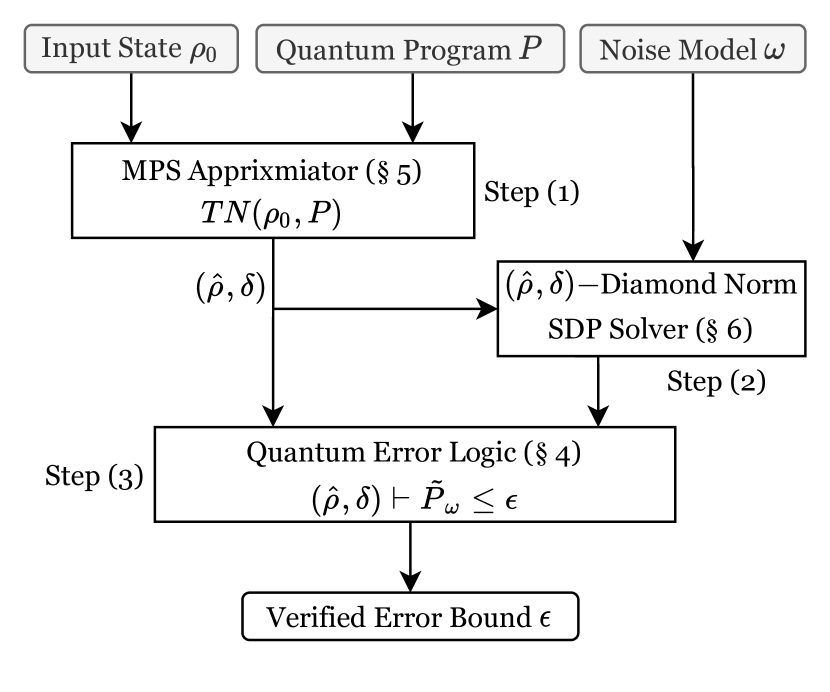
Figure 4. Gleipnir workflow.

$$\displaystyle{\hbox{}\over\hbox{\hskip 27.85396pt\vbox{\vbox{}\hbox{\hskip-27.85394pt\hbox{\hbox{$\displaystyle\displaystyle(\hat{\rho},\delta)\vdash\widetilde{P}_{\omega}\leq 0$}}}}}} \displaystyle{\hbox{\hskip 29.77794pt\vbox{\hbox{\hskip-29.77792pt\hbox{\hbox{$\displaystyle\displaystyle\|\widetilde{\mathcal{U}}_{\omega}-\mathcal{U}\|_{(\hat{\rho},\delta)}\leq\epsilon$}}}\vbox{}}}\over\hbox{\hskip 48.00043pt\vbox{\vbox{}\hbox{\hskip-48.00041pt\hbox{\hbox{$\displaystyle\displaystyle(\hat{\rho},\delta)\vdash\ \widetilde{U}_{\omega}(q_{1},\ldots)\ \leq\epsilon$}}}}}} \displaystyle{\hbox{\hskip 121.93016pt\vbox{\hbox{\hskip-121.93015pt\hbox{\hbox{$\displaystyle\displaystyle(\hat{\rho},\delta)\vdash\widetilde{P}_{1\omega}\leq\epsilon_{1}\quad{TN}(\hat{\rho},P_{1})=(\hat{\rho}^{\prime},\delta^{\prime})\quad(\hat{\rho}^{\prime},\delta+\delta^{\prime})\vdash\widetilde{P}_{2\omega}\leq\epsilon_{2}$}}}\vbox{}}}\over\hbox{\hskip 53.70023pt\vbox{\vbox{}\hbox{\hskip-53.70021pt\hbox{\hbox{$\displaystyle\displaystyle(\hat{\rho},\delta)\vdash\ \widetilde{P}_{1\omega};\widetilde{P}_{2\omega}\ \leq\epsilon_{1}+\epsilon_{2}$}}}}}} \displaystyle{\hbox{\hskip 69.52248pt\vbox{\hbox{\hskip-69.52246pt\hbox{\hbox{$\displaystyle\displaystyle(\hat{\rho},\delta^{\prime})\vdash\widetilde{P}_{\omega}\leq\epsilon^{\prime}$}\hskip 20.00003pt\hbox{\hbox{$\displaystyle\displaystyle\epsilon^{\prime}\leq\epsilon$}\hskip 20.00003pt\hbox{\hbox{$\displaystyle\displaystyle\delta^{\prime}\geq\delta$}}}}}\vbox{}}}\over\hbox{\hskip 27.38347pt\vbox{\vbox{}\hbox{\hskip-27.38345pt\hbox{\hbox{$\displaystyle\displaystyle(\hat{\rho},\delta)\vdash\widetilde{P}_{\omega}\leq\epsilon$}}}}}} \displaystyle{\hbox{\hskip 70.36693pt\vbox{\hbox{\hskip-70.36693pt\hbox{\hbox{$\displaystyle\displaystyle(\hat{\rho}_{0},\delta)\vdash\widetilde{P}_{0\omega}\leq\epsilon$}\hskip 20.00003pt\hbox{\hbox{$\displaystyle\displaystyle(\hat{\rho}_{1},\delta)\vdash\widetilde{P}_{1\omega}\leq\epsilon$}}}}\vbox{}}}\over\hbox{\hskip 110.17102pt\vbox{\vbox{}\hbox{\hskip-110.171pt\hbox{\hbox{$\displaystyle\displaystyle(\hat{\rho},\delta)\vdash\ \Big{(}\texttt{if }q=\ket{0}\texttt{then }\widetilde{P}_{0\omega}\texttt{ else }\widetilde{P}_{1\omega}\Big{)}\ \leq(1-\delta)\epsilon+\delta$}}}}}}$$ Skip       Gate       Seq       Weaken             Meas

Figure 5. Inference rules of the quantum error logic.

To use the input quantum state to tighten the computed error bound, Gleipnir introduces a new constrained diamond norm, $(\hat{\rho},\delta)$-diamond norm, and a judgment $(\hat{\rho},\delta)\vdash\widetilde{P}_{\omega}\leq\epsilon$ to reason about the error of quantum circuits. Gleipnir uses Matrix Product State (MPS) tensor networks to approximate the quantum state and compute the predicate $(\hat{\rho},\delta)$.

Figure 4 illustrates Gleipnir’s workflow for reasoning about the error bound of some quantum program $P$ with input state $\rho_{0}$ and noise model $\omega$ of quantum gates on the target device:

1. Gleipnir first approximates the quantum state $\hat{\rho}$ and a sound overapproximation of its distance $\delta$ to the ideal state $\rho$ using MPS tensor networks $TN(\rho_{0},P)=(\hat{\rho},\delta)$ (see Section 5).

2. Gleipnir then uses the constrained $(\hat{\rho},\delta)$-diamond norm metric to bound errors of noisy quantum gates given a noise model $\omega$ of the target device. Gleipnir converts the problem of efficiently computing the $(\hat{\rho},\delta)$-diamond norm to solving a polynomial-size SDP problem, given $(\hat{\rho},\delta)$ computed in Step (1) (see Section 6).

3. Gleipnir employs a lightweight quantum error logic to compute the error bound of $\widetilde{P}_{\omega}$ using the predicate $(\hat{\rho},\delta)$ computed in Step (1) and the error bounds for all used quantum gates generated by the SDP solver in Step (2) (see Section 4).

Throughout this paper, we will return to the GHZ state circuit (Example 2.1) as our running example. This example uses the program $H(q_{0});CNOT(q_{0},q_{1})$, the input state $\ket{00}\bra{00}$, and the noise model $\omega$, describing the noisy gates $\widetilde{H}_{\omega}$ and $\widetilde{CNOT}_{\omega}$. Following the steps described above, we will use Gleipnir to obtain the final judgment of:

$$(\ket{00}\bra{00},\ 0)\vdash\Big{(}\widetilde{H}_{\omega}(q_{0})\ ;\ \widetilde{CNOT}_{\omega}(q_{0},q_{1})\Big{)}\leq\epsilon,$$

where $\epsilon$ is the total error bound of the noisy program.

4. Quantum Error Logic

We first introduce our lightweight logic for reasoning about the error bounds of quantum programs. In this section, we treat MPS tensor networks and the algorithm to compute the $(\hat{\rho},\delta)$-diamond norm as black boxes, deferring their discussion to Sections 5 and 6, respectively.

The $(\hat{\rho},\delta)$-diamond norm is defined as follows:

$$\|\mathcal{U}-\mathcal{E}\|_{(\hat{\rho},\delta)} :=\max_{\begin{subarray}{c}\rho:\ \text{tr}(\rho)\ =\ 1,\\ \|\rho-\hat{\rho}\|_{1}\leq\delta\end{subarray}}\frac{1}{2}{\Big{\|}\mathcal{U}\otimes\mathcal{I}(\rho)-\mathcal{E}\otimes\mathcal{I}(\rho)\Big{\|}_{1}}.$$

That is a diamond norm with the additional constraint that the ideal input density matrix of $\rho$ needs to be within distance $\delta$ of $\hat{\rho}$, i.e., $T(\rho,\hat{\rho})\leq\delta$.

We use the judgment $(\hat{\rho},\delta)\vdash\widetilde{P}_{\omega}\leq\epsilon$ to convey that when running the noisy program $\widetilde{P}_{\omega}$ on an input state whose trace distance is at most $\delta$ from $\hat{\rho}$, the trace distance between the noisy and noiseless outputs of program $P$ is at most $\epsilon$ under the noise model $\omega$ of the underlying device.

Figure 5 presents the five inference rules for our quantum error logic. The Skip rule states that an empty program does not produce any noise. The Gate rule states that we can bound the error of a gate step by calculating the gate’s $(\hat{\rho},\delta)$-diamond norm under the noise model $\omega$. The Weaken rule states that the same error bound holds when we strengthen the precondition with a smaller approximation bound $\delta^{\prime}$. The Seq rule states that the errors of a sequence can be summed together with the help of the tensor network approximator ${TN}$. The Meas rule bounds the error in an if statement, with $\delta$ probability that the result of measuring the noisy input differs from measuring state $\rho$, causing the wrong branch to be executed. Otherwise, the probability that the correct branch is executed is $1-\delta$. Given that in both branches, the error is bounded by a uniform value $\epsilon$, we multiply this probability by the error incurred in the branch, and add it to the probability of taking the incorrect branch, to obtain the error incurred by executing a quantum conditional statement. The precondition in each branch is defined as $\hat{\rho}_{0}=M_{0}\hat{\rho}M_{0}^{\dagger}/\text{tr}(M_{0}\hat{\rho}M_{0}^{\dagger})$ and $\hat{\rho}_{1}=M_{1}\hat{\rho}M_{1}^{\dagger}/\text{tr}(M_{1}\hat{\rho}M_{1}^{\dagger})$.

Our error logic contains two external components: (1) $TN(\rho,P)=(\hat{\rho},\delta)$, the tensor network approximator used to approximate $[\![P]\!](\rho)$, obtaining $\hat{\rho}$ and an approximation error bound $\delta$; and (2) $\|\cdot\|_{(\hat{\rho},\delta)}$, the $(\hat{\rho},\delta)$-diamond norm that characterizes the error bound generated by a single gate under the noise model $\omega$. The algorithms used to compute these components are explained in Sections 5 and 6, while the soundness proof of our inference rules is given in Appendix A.

We demonstrate how these rules can be applied to the 2-qubit GHZ state circuit from Example 2.1 as follows. The program is $\widetilde{H}_{\omega}(q_{0});\widetilde{CNOT}_{\omega}(q_{0},q_{1})$ and the input state in the density matrix form is $\rho=\ket{00}\bra{00}$. We first compute the constrained diamond norm $\epsilon_{1}=\|\widetilde{\mathcal{H}}_{\omega}-\mathcal{H}\|_{(\rho,0)}$ and apply the Gate rule to obtain:

$$(\rho,0)\vdash\widetilde{H}_{\omega}(q_{0})\leq\epsilon_{1}.$$

Then, we use the tensor network approximator to compute ${TN}(\rho,H(q_{0}))$, whose result is $(\hat{\rho},\delta)$. Using such a predicate, we compute the $(\hat{\rho},\delta)$-diamond norm $\epsilon_{2}=\|\widetilde{\mathcal{CNOT}}_{\omega}-\mathcal{CNOT}\|_{(\hat{\rho},\delta)}$. Applying the Gate rule again, we obtain:

$$(\hat{\rho},\delta)\vdash\widetilde{CNOT}_{\omega}(q_{0},q_{1})\leq\epsilon_{2}.$$

Finally, we apply the Seq rule:

$$(\rho,0)\vdash\Big{(}\widetilde{H}_{\omega}(q_{0});\widetilde{CNOT}_{\omega}(q_{0},q_{1})\Big{)}\leq\epsilon_{1}+\epsilon_{2},$$

which gives the error bound of the noisy program, $\epsilon_{1}+\epsilon_{2}$.

5. Quantum State Approximation

Gleipnir uses tensor networks to adaptively compute the constraints of the input quantum state using an approximate state $\hat{\rho}$ and its distance $\delta$ from the ideal state $\rho$. We provide the background on tensor networks in Section 5.1, present how we use tensor networks to approximate quantum states in Section 5.2, and give examples in Section 5.3.

5.1. Tensor network

Tensors. Tensors describe the multilinear relationship between sets of objects in vector spaces, and can be represented by multi-dimensional arrays. The rank of a tensor indicates the dimensionality of its array representation: vectors have rank $1$, matrices rank $2$, and superoperators rank $4$ (since they operate over rank $2$ density matrices).

Contraction. Tensor contraction generalizes vector inner products and matrix multiplication. A contraction between two tensors specifies an index for each tensor, sums over these indices, and produces a new tensor. The two indices used to perform contraction must have the same range to be contracted together. The contraction of two tensors with ranks $a$ and $b$ will have rank $a+b-2$; for example, if we contract the first index in $3$-tensor $A$ and the second index in $2$-tensor $B$, the output will be a 3-tensor:

$$(A\times_{1,2}B)[jkl]=\sum_{t}A[tjk]B[lt].$$

Tensor product. The tensor product is calculated like an outer product; if two tensors have ranks $a$ and $b$ respectively, their tensor product is a rank $a+b$ tensor. For example, the tensor product of 2-tensor $A$ and 2-tensor $B$ is a 4-tensor:

$$(A\otimes B)[ijkl]=A[ij]B[kl].$$

Tensor networks. Tensor network (TN) representation is a graphical calculus for reasoning about tensors, with an intuitive representation of various quantum objects. Introduced in the 1970s by Penrose (Penrose, 1971), this notation is used in quantum information theory (Vidal, 2008, 2003; Evenbly and Vidal, 2009; Verstraete et al., 2008; Wood et al., 2011; Schollwöck, 2005), as well as in other fields such as machine learning (Efthymiou et al., 2019; Stoudenmire and Schwab, 2016).

(a) Vector
(rank 1)

(b) Matrix
(rank 2)

(c) Superoperator
(rank 4)

Figure 6. Tensor network representation of various tensors.

As depicted in Figure 6, tensor networks consist of nodes and edges. Each node represents a tensor, and each edge out of the node represents an index of the tensor. As illustrated in Figure 7, the resulting network will itself constitute a whole tensor, with each open-ended edge representing one index for the final tensor. The graphical representation of a quantum program can be directly interpreted as a tensor network. For example, the 2-qubit GHZ state circuit in Figure 2 can be represented by a tensor network in Figure 8.

(a) Matrix multiplication $AB$

(b) Outer product $\ket{\psi}\bra{\psi}$

Figure 7. Tensor network representation for two matrix operations. In general, tensor contractions are represented by linking edges, and tensor products by juxtaposition.

(a) Quantum circuit.

(b) Tensor network.

Figure 8. The GHZ state, represented as a quantum circuit (a) and a tensor network (b). When we evaluate the output of the circuit, we can see that the input state $\ket{00}$ (enclosed in the dashed blue box), the $H$ gate $H\otimes I$ (enclosed in the dashed red box), and the $CNOT$ gate (enclosed in the dashed brown box). When evaluating the tensor network in (b), the output is the same as the program output, $\big{(}\ket{00}+\ket{11}\big{)}/\sqrt{2}$.

	Gate	Superoperator	Singular Value
	Contraction	Application	Decomposition
Tensor network
Dirac notation	$U\ket{\psi}=\ket{\phi}$	$\mathcal{E}(\rho)=\hat{\rho}$	$M=\sum_{j}\sigma_{j}U\ket{j}\bra{j}V^{\dagger}$
Rank	1	2	2

Table 1. Examples of tensor network transformations for basic quantum operations.

Transforming tensor networks. To speed up the evaluation of a large tensor network, we can apply reduction rules to transform and simplify the network structure. In Table 1, we summarize some common reduction rules we use. The Gate Contraction rule transforms a vector $\psi$ and a matrix $U$ connected to it into a new vector $\phi$ that is the product of $U$ and $\psi$. The Superoperator Application rule transforms a superoperator $\mathcal{E}$ and a matrix $\rho$ connected to it into a matrix $\hat{\rho}$ that represents the application of the superoperator $\mathcal{E}$ to $\rho$. The Singular Value Decomposition (SVD) rule transforms a matrix $M$ into the product of three matrices: $U$, $\Sigma$, and $V^{\dagger}$, where $\Sigma$ is a diagonal matrix whose diagonal entries are the singular values $\sigma_{1},\ldots,\sigma_{n}$ of $M$. This special matrix $\Sigma=\sum_{j}\sigma_{j}\ket{j}\bra{j}$ is graphically represented by a diamond. By dropping small singular values in the diagonal matrix $\Sigma$, we can obtain a simpler tensor network which closely approximates the original one.

5.2. Approximate quantum states

In this section, we describe our tensor network approximator algorithm computing ${TN}(\rho,P)=(\hat{\rho},\delta)$, such that the trace distance between our approximation $\hat{\rho}$ and the perfect output $[\![P]\!](\rho)$ satisfies ${T}\big{(}\hat{\rho},[\![P]\!](\rho)\big{)}\leq\delta$. At each stage of the algorithm, we use Matrix Product State (MPS) tensor networks (Perez-Garcia et al., 2007) to approximate quantum states. This class of tensor networks uses $2n$ matrices to represent $2^{n}$-length vectors, greatly reducing the computational cost. MPS tensor networks take a size $w$ as an argument, which determines the space of representable states. When $w$ is not large enough to represent all possible quantum states, the MPS is an approximate quantum state whose approximation bound depends on $w$. The MPS representation with size $w$ of a quantum state $\psi$ (represented as a vector) is:

$$\ket{\psi}_{\text{MPS}}:=\sum_{i_{1},\ldots,i_{n}}A_{1}^{(i_{1})}A_{2}^{(i_{2})}\cdots A_{n}^{(i_{n})}\ket{i_{1}i_{2}\cdots i_{n}},$$

where $A_{1}^{(i_{1})}$ is a row vector of dimension $w$, $A_{2}^{(i_{2})},\ldots,A_{n-1}^{(i_{n-1})}$ are $w\times w$ matrices, and $A_{n}^{(i_{n})}$ is a column vector of dimension $w$. We use $i_{j}$ to represent the value of a basis $\ket{i_{1}i_{2}\cdots i_{n}}$ at position $j$, which can be $0$ or $1$. For example, to represent the 3-qubit state $\big{(}\ket{000}+\ket{010}+\ket{001}\big{)}/3$ in MPS, we must find matrices $A_{1}^{(0)},A_{1}^{(1)},A_{2}^{(0)},A_{2}^{(1)},A_{3}^{(0)},A_{3}^{(1)}$ such that

$$A_{1}^{(0)}A_{2}^{(0)}A_{3}^{(0)}=A_{1}^{(0)}A_{2}^{(1)}A_{3}^{(0)}=A_{1}^{(0)}A_{2}^{(0)}A_{3}^{(1)}=\frac{1}{3},$$

while $A_{1}^{(i_{1})}A_{2}^{(i_{2})}A_{3}^{(i_{3})}=0$ for all $(i_{1},i_{2},i_{3})\neq(0,0,0)$, $(0,1,0)$, or $(0,0,1)$.

$A_{i}^{(0)}$ and $A_{i}^{(1)}$ can be taken together as a 3-tensor $A_{i}$ ($A_{1}$ and $A_{n}$ are 2-tensors) where the superscript is taken as the third index besides the two indices of the matrix. Overall, the MPS representation can be seen as a tensor network, as shown in Figure 9. $A_{1},\ldots,A_{n}$ are linked together in a line, while $i_{1},\ldots,i_{n}$ are open wires.

Figure 9. The MPS representation of six qubits.

Our approximation algorithm starts by initializing the MPS to the input state in vector form. Then, for each gate of the quantum program, we apply it to the MPS to get the intermediate state at this step and compute the distance between MPS and the ideal state. Since MPS only needs to maintain $2n$ tensors, i.e., $A_{1}^{(0)}$, $A_{1}^{(1)}$, $A_{2}^{(0)}$, $A_{2}^{(1)}$, $\cdots$, $A_{n}^{(0)}$, $A_{n}^{(1)}$, this procedure can be performed efficiently with polynomial running time. After applying all quantum gates, we obtain an MPS that approximates the output state of the quantum program, as well as an approximation bound by summing together all accumulated approximation errors incurred by the approximation process. Our approximation algorithm consists of the following stages.

Initialization. Let $\ket{s_{1}s_{2}\cdots s_{n}}$ be the input state for an $n$-qubit quantum circuit. For all $k\in[1,n]$, we initialize $A_{k}^{(s_{k})}=E$ and $A_{k}^{(1-s_{k})}=0$, where $E$ is the matrix that $E_{1,1}=1$ and $E_{i,j}=0$ for all $i\neq 1$ or $j\neq 1$.

Applying 1-qubit gates. Applying a 1-qubit gate on an MPS always results in an MPS and thus does not incur any approximation error. For a single-qubit gate $G$ on qubit $i$, we update the tensor $A_{i}$ to $A^{\prime}_{i}$ as follows:

$${A^{\prime}}_{i}^{(s)}=\sum_{s^{\prime}\in\{0,1\}}G_{ss^{\prime}}A_{i}^{(s^{\prime})}\qquad\text{for }s=0\text{ or }1.$$

In the tensor network representation, such application amounts to contracting the tensor for the gate with $A_{i}$ (see Figure 10).

Figure 10. Applying a 1-qubit gate to an MPS. We contract the MPS node for the qubit and the gate (in the dashed box), resulting in another 3-tensor MPS node.

Figure 11. Applying a 2-qubit gate on two adjacent qubits to the MPS, via (i) node contraction, (ii) singular value decomposition, and (iii) singular value truncation with re-normalization.

Applying 2-qubit gates. If we are applying a 2-qubit gate $G$ on two adjacent qubits $i$ and $i+1$, we only need to modify $A_{i}$ and $A_{i+1}$. We first contract $A_{i}$ and $A_{i+1}$ to get a $2w\times 2w$ matrix $M$:

$$\begin{bmatrix}A_{i}^{(0)}\\ A_{i}^{(1)}\end{bmatrix}\begin{bmatrix}A_{i+1}^{(0)}&A_{i+1}^{(1)}\end{bmatrix}=\begin{bmatrix}M_{00}&M_{01}\\ M_{10}&M_{11}\end{bmatrix}=M.$$

Then, we apply the 2-qubit gate to it:

$$M_{ij}^{\prime}=\sum_{k,l}G_{ijkl}M_{kl}.$$

We then need to decompose this new matrix $M^{\prime}$ back into two tensors. We first apply the Singular Value Decomposition rule on the contracted matrix:

$$M^{\prime}=U\Sigma V^{\dagger}.$$

When $w$ is not big enough to represent all possible quantum states, $M^{\prime}$ introduces approximation errors and may not be a contraction of two tensors. Thus, we truncate the lower half of the singular values in $\Sigma$, enabling the tensor decomposition while reducing the error:

$$\Sigma\approx\begin{bmatrix}\Sigma^{\prime}&0\\ 0&0\end{bmatrix}.$$

Therefore, we arrive at a new MPS whose new tensors $A^{\prime}_{i}$ and $A^{\prime}_{i+1}$ are calculated as follows:

$$\begin{bmatrix}A_{i}^{(0)^{\prime}}&*\\ A_{i}^{(1)^{\prime}}&*\end{bmatrix}=U,\begin{bmatrix}A_{i+1}^{(0)^{\prime}}&A_{i+1}^{(1)^{\prime}}\\ *&*\end{bmatrix}=\Sigma^{\prime}V,$$

where $*$ denotes the part that we truncate. After truncation, we renormalize the state to a norm-$1$ vector.

Figure 11 shows the above procedure in tensor network form by (1) first applying Gate Contracting rule for $A_{i}$, $A_{i+1}$ and $G$, (2) using Singular Value Decomposition rule to decompose the contracted tensor, (3) truncating the internal edge to width $w$, and finally (4) calculating the updated $A^{\prime}_{i}$ and $A^{\prime}_{i+1}$. If we want to apply a 2-qubit gate to non-adjacent qubits, we add swap gates to move the two qubits together before applying the gate to the now adjacent pair of qubits.

Bounding approximation errors. When applying 2-qubit gates, we compute an MPS to approximate the gate application. Each time we do so, we must bound the error due to this approximation. Since the truncated values themselves comprise an MPS state, we may determine the error by simply calculating the trace distance between the states before and after truncation.

The trace distance of two MPS states can be calculated from the inner product of these two MPS:

$$\delta:=\big{|}\ket{\phi}\bra{\phi}-\ket{\psi}\bra{\psi}\big{\|}_{1}=2\sqrt{1-|\braket{\phi}{\psi}|^{2}}.$$

The inner product of two states $\ket{\psi}$ and $\ket{\phi}$ (represented using $A$ and $B$ in their MPS forms) is defined as follows:

$$\braket{\psi}{\phi}= \sum_{i_{1},\ldots,i_{n}}\Big{\langle}A_{1}^{(i_{1})}\cdots A_{n}^{(i_{n})},B_{1}^{(i_{1})}\cdots B_{n}^{(i_{n})}\Big{\rangle}.$$

Figure 12 shows its tensor network graphical representation.

Figure 12. Tensor network representation of the inner product of two MPSs. An open wire of one MPS is linked with an open wire of another, which denotes the summation over $i_{1},\ldots,i_{n}$.

In our approximation algorithm, we can iteratively calculate from qubit $1$ to qubit $n$ the distance by first determining:

$$D_{1}=A_{1}^{(0)}B_{1}^{(0){\dagger}}+A_{1}^{(1)}B_{1}^{(1){\dagger}}.$$

Then, we repeatedly apply tensors to the rest of qubits:

$$D_{i}=A_{i}^{(0)}D_{i-1}B_{i}^{(0){\dagger}}+A_{i}^{(1)}D_{i-1}B_{i}^{(1){\dagger}},$$

leading us to the final result of $D_{n}=\braket{\psi}{\phi}$. In the tensor network graphical representation, this algorithm is a left-to-right contraction, as shown in Figure 13.

Figure 13. Contraction of the inner product of two MPS. We first contract $A_{1}$ and $B_{1}$ to get $D_{1}$. Then contract $D_{1}$, $A_{2}$ and $B_{2}$ to $D_{2}$. And then $D_{2},A_{3}$ and $B_{3}$ to $D_{3}$. Repeating this process will result in a single tensor node $D_{n}$, i.e., the final answer.

Given the calculated distance of each step, we must combine them to obtain the overall approximation error. For some arbitrary quantum program with $t$ 2-qubit gates, let the truncation errors be $\delta_{1},\delta_{2},\ldots,\delta_{t}$ when applying the 2-qubit gates $g_{1},g_{2},...,g_{t}$, the final approximation error is $\delta=\sum_{i=1}^{t}\delta_{i}$.

To see why, we consider the approximation of one 2-qubit gate. Let $\ket{\psi}$ denote some quantum state and $\ket{\hat{\psi}}$ its approximation with bounded error $\delta_{0}$. After applying a 2-qubit gate $G$ to the approximate MPS state, we obtain the truncated result $\ket{{\phi}}$ with bounded error $\delta_{1}$. We now have:

$$\|G\ket{\psi}-\ket{\phi}\| \leq\|G\ket{\psi}-G\ket{\hat{\psi}}\|\ +\ \|G\ket{\hat{\psi}}-\ket{\phi}\|$$

$$=\|\ket{\psi}-\ket{\hat{\psi}}\|\ +\ \|G\ket{\hat{\psi}}-\ket{\phi}\|$$

(1) $$=\delta_{0}+\delta_{1},$$

where $\|\ket{\psi}-\ket{\phi}\|=\|\ket{\psi}\bra{\psi}-\ket{\phi}\bra{\phi}\|_{1}$. The inequality holds because of the triangular inequality of quantum state distance and the fact that $G$ is unitary, thus preserving the trace norm. Repeating this for each step, we know that the total approximation error is bounded by the sum of all approximation errors.

Supporting branches. Due to the deferred measurement principle (Nielsen and Chuang, 2011), measurements can always be delayed to the end of the program. Thus, in-program measurements are not required for quantum program error analysis. Our approach can also directly support if statements by calculating an MPS for each branch. When we apply the measurement on the $i$-th qubit, we obtain the collapsed states by simply setting $A_{i}^{(0)}$ or $A_{i}^{(1)}$ to the zero matrix, obtaining MPS tensor networks corresponding to measurements of $0$ and $1$. Using these states, we continue to evaluate the subsequent MPS in each branch separately. We cannot merge the measured states once they have diverged, so we must duplicate any code sequenced after the branch and compute the approximated state separately; the number of intermediate MPS representations we must compute is thus the number of branches. The overall approximation error is taken to be the sum of approximation errors incurred on all branches. Note that the number of branches may be exponential to the number of if statements.

Complexity analysis. The running time of all the operations above scales polynomially with respect to the MPS size $w$, number of qubits $n$, number of branches $b$, and number of gates $m$ in the program. To be precise, applying a 1-qubit gate only requires one matrix addition with a $O(w^{2})$ time complexity. Applying a 2-qubit gate requires matrix multiplication and SVD with a $O(w^{3})$ time complexity. Computing inner product of two MPS (e.g. for contraction) requires $O(n)$ of matrix multiplications, incurring an overall running time of $O(nw^{3})$. Since the algorithm scans all $m$ gates in the program, the overall time complexity is $O(bmnw^{3})$.

Although a perfect approximation (i.e., a full simulation) requires an MPS size that scales exponentially with respect to the number of qubits (i.e., $2^{n}$ size when there are $n$ qubits), our approximation algorithm allows Gleipnir to be configured with smaller MPS sizes, sacrificing some precision in favor of efficiency and enabling its practical use for real-world quantum programs.

Correctness. From the quantum program semantics defined in Figure 3, we know that we can compute the output state by applying all the program’s gates in sequence. Following Equation (1), we know that the total error bound for our approximation algorithm is bounded by the sum of each step’s bound. Thus, we can conclude that our algorithm correctly approximates the output state and correctly bounds the approximation error in doing so.

Theorem 5.1.

Let the output of our approximation algorithm be $(\hat{\rho},\delta)=\mathrm{TN}(\rho,P)$. The trace distance between the approximation and perfect output is bound by $\delta$:

$${\Big{\|}[\![P]\!](\hat{\rho})-[\![P]\!](\rho)\Big{\|}_{1}}\leq\delta.$$

5.3. Example: GHZ circuit

We revisit the GHZ circuit in Figure 2 to walk through how we approximate quantum states with MPS tensor networks. The same technique can be applied to larger and more complex quantum circuits, discussed in Section 7.

Approximation using 2-wide MPS. Since the program only contains two qubits, an MPS with size $w=2$ can already perfectly represent all possible quantum states such that no approximation error will be introduced. Assume the input state is $\ket{00}$. First, we initialize all the tensors based on the input state $\ket{00}$:

$$A_{1}^{(0)}=[1,0],\ A_{1}^{(1)}=[0,0],\ A_{2}^{(0)}=[1,0]^{T},\ A_{2}^{(1)}=[0,0]^{T}.$$

Then, we apply the first $H$ gate to qubit 1, changing only $A_{1}^{(0)}$ and $A_{1}^{(1)}$:

$A_{1}^{(0)}=[1,0]/\sqrt{2}$,

$A_{1}^{(1)}=[1,0]/\sqrt{2}$.

To apply the CNOT gate on qubit $1$ and $2$, we first compute matrix $M$ and $M^{\prime}$:

$$M=\begin{bmatrix}1/\sqrt{2}&0\\ 1/\sqrt{2}&0\end{bmatrix},\quad M^{\prime}=\begin{bmatrix}1/\sqrt{2}&0\\ 0&1/\sqrt{2}\end{bmatrix}.$$

We then decompose $M^{\prime}$ using SVD,

$$U=V^{\dagger}=\begin{bmatrix}1&0\\ 0&1\end{bmatrix},\quad\Sigma=\begin{bmatrix}1/\sqrt{2}&0\\ 0&1/\sqrt{2}\end{bmatrix}.$$

Because there are just 2 non-zero singular values, we do not need to drop singular values with 2-wide MPS networks and can compute the new MPS as follows:

$A_{1}^{(0)}=[1,0]$,	$A_{1}^{(1)}=[0,1]$,
$A_{2}^{(0)}=[1/\sqrt{2},0]^{T}$,	$A_{2}^{(1)}=[0,1/\sqrt{2}]^{T}$.

We can see that the output will be $\hat{\rho}=\frac{\ket{00}+\ket{11}}{\sqrt{2}}$ and $\delta=0$, since $A_{1}^{(0)}A_{2}^{(0)}=A_{1}^{(1)}A_{2}^{(1)}=1/\sqrt{2}$ and other values of $i_{0}$ and $i_{1}$ result $0$.

Approximation using 1-wide MPS. To show how we calculate the approximation error, we use the simplest form of MPS with size $w=1$, while each $A_{i}^{(j)}$ becomes a number.

We first initialize the MPS to represent $\ket{00}$:

$$A_{1}^{(0)}=1,\ A_{1}^{(1)}=0,\ A_{2}^{(0)}=1,\ A_{2}^{(1)}=0.$$

Then, we apply the $H$ gate to qubit 1:

$$A_{1}^{(0)}=1/\sqrt{2},\ A_{1}^{(1)}=1/\sqrt{2},\ A_{2}^{(0)}=1,\ A_{2}^{(1)}=0.$$

After that, we apply the CNOT gate and compute $M$ and $M^{\prime}$:

$$M=\begin{bmatrix}1/\sqrt{2}&0\\ 1/\sqrt{2}&0\end{bmatrix},\quad M^{\prime}=\begin{bmatrix}1/\sqrt{2}&0\\ 0&1/\sqrt{2}\end{bmatrix}.$$

We decompose $M^{\prime}$ using SVD:

$$U=V^{\dagger}=\begin{bmatrix}1&0\\ 0&1\end{bmatrix},\quad\Sigma=\begin{bmatrix}1/\sqrt{2}&0\\ 0&1/\sqrt{2}\end{bmatrix}.$$

Since there are 2 non-zero singular values, we have to drop the lower half with 1-wide MPS tensor networks. Finally, we obtain $A^{\prime}_{1}$ and $A^{\prime}_{2}$:

$$A_{1}^{(0)}=1,\ A_{1}^{(1)}=0,\ A_{2}^{(0)}=1/\sqrt{2},\ A_{2}^{(1)}=0.$$

We renormalize the MPS:

$$A_{1}^{(0)}=1,\ A_{1}^{(1)}=0,\ A_{2}^{(0)}=1,\ A_{2}^{(1)}=0.$$

Thus, the output approximate state is $\ket{00}$.

To calculate the approximation error bound, we represent the part we drop as an MPS $B$:

$$B_{1}^{(0)}=0,\ B_{1}^{(1)}=1,\ B_{2}^{(0)}=0,\ B_{2}^{(1)}=\sqrt{2}.$$

Let the unnormalized final state be $\ket{A}$ and the dropped state be $\ket{B}$. Then, the final output is $\sqrt{2}\ket{A}$ and the ideal output is $\ket{A}+\ket{B}$. The trace distance between the state is

$$\delta=2\sqrt{1-|\braket{\sqrt{2}A}{A+B}^{2}|}=\sqrt{2}.$$

Therefore, the final output will be $\hat{\rho}=\ket{00}\bra{00}$ and $\delta=\sqrt{2}$.

6. Computing the $(\hat{\rho},\delta)$-Diamond Norm

Section 4 introduces our quantum error logic using the $(\hat{\rho},\delta)$-diamond norm, while treating its computation algorithm as a black box. In this section, we describe how to efficiently calculate the $(\hat{\rho},\delta)$-diamond norm given $(\hat{\rho},\delta,\mathcal{U},\mathcal{E})$, where $\mathcal{U}$ and $\mathcal{E}$ are the perfect and the noisy superoperators respectively.

Constrained diamond norm. In $(\hat{\rho},\delta)$-diamond norm, the input state $\rho_{\text{in}}$ is constrained by

$$\|\hat{\rho}-\rho_{\text{in}}\|_{1}\leq\delta.$$

We first compute the local density matrix (defined later in this section) $\rho^{\prime}$ of $\hat{\rho}$. Then, to compute the $(\hat{\rho},\delta)$-diamond norm, we extend the result of Watrous (Watrous, 2013) by adding the following constraint:

$$\text{tr}(\rho^{\prime}\rho)\geq\|\rho^{\prime}\|_{F}(\|\rho^{\prime}\|_{F}-\delta),$$

where $\rho$ denotes the local density matrix of $\rho_{\text{in}}$. Thus, $(\hat{\rho},\delta)$-diamond norm can be computed by the following semi-definite program(SDP):

Theorem 6.1.

The $(\hat{\rho},\delta)$-diamond norm $||\Phi||_{(\hat{\rho},\delta)}$ can be solved by the semi-definite program(SDP) in Equation (2).

(2) $$\begin{array}[]{ll@{}ll}\text{maximize}&\mathrm{tr}(J(\Phi)W)\\ \text{subject to}&I\otimes\rho\succcurlyeq W\\ &{\text{tr}(\rho^{\prime}\rho)\geq\|\rho^{\prime}\|_{F}(\|\rho^{\prime}\|_{F}-\delta)}\\ &W\succcurlyeq 0,\ \rho\succcurlyeq 0,\ \mathrm{tr}(\rho)=1,\end{array}$$

where $J$ is the Choi-Jamiolkowski isomorphism (Choi, 1975) and $\Phi=\mathcal{U}-\mathcal{E}.$

Proof.

Given $(\hat{\rho},\delta)$, we know that $\|\hat{\rho}-\rho_{\text{in}}\|_{1}\leq\delta$, where $\rho_{\text{in}}$ is the real input state. Let $\rho^{\prime}$ and $\rho$ be the local density operator of $\hat{\rho}$ and $\rho_{\text{in}}$. Because partial trace can only decrease the trace norm, we know that

$$\|\rho^{\prime}-\rho\|_{1}\leq\|\hat{\rho}-\rho_{\text{in}}\|_{1}\leq\delta.$$

For a matrix $\rho$, let $\|\rho\|_{F}$ be the Frobenius norm which is the square root of the sum of the squares of all elements in a matrix. Because $\|\rho\|_{F}\leq\|\rho\|_{1}$ for all $\rho$, we know that $\|\rho^{\prime}-\rho\|_{F}\leq\delta$. Then, we have

$$\text{tr}(\rho^{\prime}\rho) =\text{tr}(\rho^{2})+\text{tr}((\rho^{\prime}-\rho)\rho)$$

$$=\|\rho^{\prime}\|_{F}^{2}+\text{tr}((\rho^{\prime}-\rho)\rho)$$

$$\geq\|\rho^{\prime}\|_{F}^{2}-\|\rho^{\prime}\|_{F}\|\rho^{\prime}-\rho\|_{F}$$

$$\geq\|\rho^{\prime}\|_{F}(\|\rho^{\prime}\|_{F}-\delta),$$

where the third step holds because of the Cauchy-Schwarz inequality.

Because the $(Q,\lambda)$-diamond norm can be solved by the following SDP by adding a constraint $\text{tr}(Q\rho)\geq\lambda$ (Hung et al., 2019):

$$\begin{array}[]{ll@{}ll}\text{maximize}&\mathrm{tr}(J(\Phi)W)\\ \text{subject to}&I\otimes\rho\succcurlyeq W\\ &{\text{tr}(Q\rho)\geq\lambda}\\ &W\succcurlyeq 0,\ \rho\succcurlyeq 0,\ \mathrm{tr}(\rho)=1.\end{array}$$

$(\hat{\rho},\delta)$-diamond norm can thus be calculated by the SDP (2). ∎

Let the solved, optimal value of SDP in Equation (2) be $\epsilon$. We conclude that the $(\hat{\rho},\delta)$-diamond norm must be bounded by $\epsilon$, i.e.,

$$\|\Phi\|_{(\hat{\rho},\delta)}\leq\epsilon.$$

SDP size. The size of the SDP in Equation (2) is exponential with respect to the maximum number of quantum gates’ input qubits. Since near-term (NISQ) quantum computers are unlikely to support quantum gates with greater than two input qubits, we can treat the size of the SDP problem as a constant, for the purposes of discussing its running time. Because the running time of solving an SDP scales polynomially with the size of the SDP, the running time to calculate $(\hat{\rho},\delta)$-diamond norm can be seen as a constant.

Computing local density matrix. The local density matrix (also known as reduced density matrix (Nielsen and Chuang, 2011)) represents the local information of a quantum state. It is defined using a partial trace on the (global) density for the part of the state we want to observe. For example, the local density operator on the first qubit of $\frac{\ket{00}+\ket{11}}{\sqrt{2}}$ is $\frac{1}{2}\begin{pmatrix}1&1\\ 1&1\end{pmatrix}$, meaning that the first qubit of the state is half $\ket{0}$ and half $\ket{1}$.

In Equation (2), we need to compute the local density matrix $\rho^{\prime}$ of $\hat{\rho}$ about the qubit(s) that the noise represented by $\Phi$ acts on. $\hat{\rho}$ is represented by an MPS. The calculation of a local density operator of an MPS works similarly to how we calculate inner products, except the wire $i_{k}$ where $k$ is a qubit that we want to observe.

7. Evaluation

	Qubit	Gate	Gleipnir bound	Running	LQR (Hung et al., 2019) with	Running	Worst-case
Benchmark	number	count	($\times 10^{-4}$)	time (s)	full simulator ($\times 10^{-4}$)	time (s)	bound ($\times 10^{-4}$)
QAOA_line_10	10	27	0.05	2.77	0.05	215.2	27
Isingmodel10	10	480	335.6	31.6	335.6	4701.8	480
QAOARandom20	20	160	136.6	19.8	-	(timed out)	160
QAOA4reg_20	20	160	138.8	12.5	-	(timed out)	160
QAOA4reg_30	30	240	207.0	25.8	-	(timed out)	240
Isingmodel45	45	2265	1739.4	338.0	-	(timed out)	2265
QAOA50	50	399	344.1	58.7	-	(timed out)	399
QAOA75	75	597	517.2	113.7	-	(timed out)	597
QAOA100	100	677	576.7	191.9	-	(timed out)	677

Table 2. Experimental results of Gleipnir ($w=128$) and the baseline on different quantum programs, showing the bounds given by Gleipnir’s $(\hat{\rho},\delta)$-diamond norm, the $(Q,\lambda)$-diamond norm with full simulation, and the worst case bound given by unconstrained diamond norm. Experiments time out if they run for longer than 24 hours. Note that the worst case bound is directly proportional to the number of gates.

This section evaluates Gleipnir on a set of realistic near-term quantum programs. We compare the bounds given by Gleipnir to the bounds given by other methods, as well as the error we experimentally measured from an IBM’s real quantum device. All approximations and full simulations are performed on an Ubuntu 18.04 server with an Intel Xeon W-2175 (28 cores @ 4.3 GHz), 62 GB memory, and a 512 GB Intel SSD Pro 600p.

7.1. Evaluating the computed error bounds

We evaluated Gleipnir on several important quantum programs, under a sample noise model containing the most common type of quantum noises. We compared the bounds produced by Gleipnir with the LQR’s $(Q,\lambda)$-diamond norm with full simulation and the worse-case bounds given by the unconstrained diamond norm.

Noise model. In our experiments, our quantum circuits are configured such that each noisy 1-qubit gate has a bit flip ($X$) with probability $p=10^{-4}$:

$$\Phi(\rho)=(1-p)\rho+pX\rho X.$$

Each 2-qubit gate also has a bit flip on its first qubit.

Framework configuration. For the approximator, we can adjust the size of the MPS network, depending on available computational resources; the larger the size, the tighter error bound. In all experiments, we use an MPS of size 128.

Baseline. To evaluate the error bounds given by Gleipnir, we first compared them with the worst-case bounds calculated using the unconstrained diamond norm (see Section 2.3). For each noisy quantum gate, we compute its unconstrained diamond norm distance to the perfect gate and obtain the worst-case bound by summing all unconstrained diamond norms. The unconstrained diamond norm distance of a bit-flipped gate and a perfect gate is given by:

$$\|\Phi-I\|_{\diamond}\quad =\quad\|(pX\circ X+(1-p)I)-I\|_{\diamond}$$

$$=\quad p\|X\circ X-I\|_{\diamond}$$

$$=\quad p,$$

where $X\circ X$ denotes the function that maps $\rho$ to $X\rho X$. Therefore, the total noise is bounded by $np$, where $n$ is the number of noisy gates, due to additivity of diamond norms. Because every gate has a noise, the worst case bound produced by unconstrained diamond norm is simply proportional to the number of gates in the program.

We also compare our error bound with what we obtain from LQR (Hung et al., 2019) using a full quantum program simulator to generate best quantum predicate. This approach’s running time is exponential to the number of qubits and times out (runs for longer than 24 hours) on programs with $\geq 20$ qubits.

Programs. We analyzed two classes of quantum programs that are expected to be most useful in the near-term, namely:

• The Quantum Approximate Optimization Algorithm (QAOA) (Farhi et al., 2014) that can be used to solve combinatorial optimization problems. We use it to find the max-cut for various graphs with qubit sizes from 10 to 100.

• The Ising model (Quantum et al., 2020)—a thermodynamic model for magnets widely used in quantum mechanics. We run the Ising model with sizes 10 and 45.

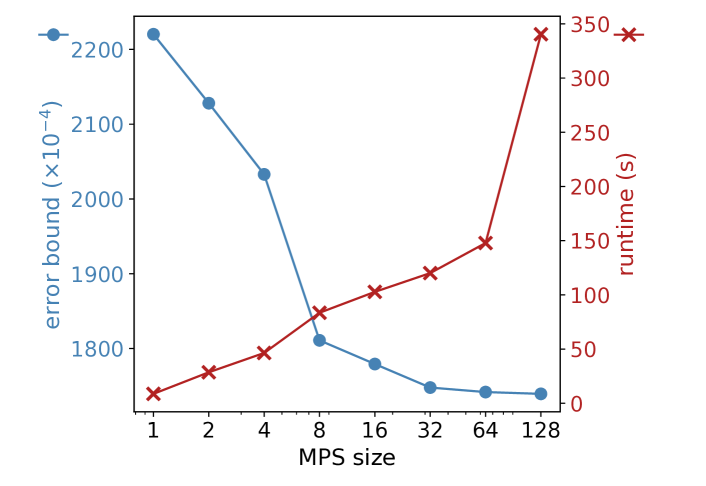
Figure 14. The error bounds and runtimes of Gleipnir on the program Isingmodel45 with different MPS sizes.

Evaluation. Table 2 presents the evaluation results. We can see that Gleipnir’s bounds are $15\%\sim 30\%$ tighter than what the unconstrained diamond norm gives, on large quantum circuits with qubit sizes $\geq 20$. On small qubit-size circuits, our bound is as strong as the exponential-time method based on full simulation.

We also evaluated how MPS size impacts the performance of Gleipnir. As we can see for the Isingmodel45 program (see Figure 14), larger MPS sizes result in tighter error bounds, at the cost of longer running times, with marginal returns beyond a certain size. We found that MPS networks with a size of 128 performed best for our candidate programs, though in general, this parameter can be adjusted according to precision requirements and the availability of computational resources. As the MPS size grows, floating point errors become more significant, so higher precision representations are necessary for larger MPS sizes. Note that one cannot feasibly compute the precise error bound of the Isingmodel45 program, since that requires computing the $2^{45}\times 2^{45}$ matrix representation of the program’s output.

7.2. Evaluating the quantum compilation error mitigation

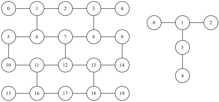
Figure 15. The coupling map of the IBM Boeblingen (left) and Lima (right) quantum computer, where each node represents a qubit. Only qubit pairs with a connecting edge can be used to implement a 2-qubit gate.

To demonstrate that Gleipnir can be used to evaluate the error mitigation performance of quantum compilers for real quantum computers today, we designed an experiment based on the noise-adaptive qubit mapping problem (Bhattacharjee et al., 2019; Murali et al., 2019). When executing a quantum program on a real quantum computer, a quantum compiler must decide which physical qubit each logical qubit should be mapped to, in accordance with the quantum computer’s coupling map (e.g., Figure 15). Since quantum devices do not have uniform noise across qubits, a quantum compiler’s mapping protocol should aim to map qubits such that the quantum program is executed with as little noise as possible.

Figure 16. The GHZ-3 circuit (left) and the GHZ-5 circuit (right).

Experiment design. We compared three different qubit mappings of the 3-qubit GHZ (GHZ-3) circuit and the 5-qubit GHZ circuit (GHZ-5) (see Figure 16): $q_{0}-q_{1}-q_{2}$, $q_{1}-q_{2}-q_{3}$, and $q_{2}-q_{3}-q_{4}$ for GHZ-3, and $q_{0}-q_{1}-q_{2}-q_{3}-q_{4}$ and $q_{2}-q_{1}-q_{0}-q_{3}-q_{4}$ for GHZ-5, where $q_{i}$ represents the $i$th physical qubit. As the baseline, we ran our circuit on a real quantum computer with each qubit mapping and measured the output to obtain a classical probability distribution. We computed the measured error by taking the statistical distance of this distribution from the distribution of the ideal output state $(\ket{000}+\ket{111})/\sqrt{2}$ and $(\ket{00000}+\ket{11111})/\sqrt{2}$. We then used Gleipnir to compute the noise bound for each mapping, based on our quantum computer’s noise model. Because the trace distance represents the maximum possible statistical distance of any measurement on two quantum states (see Section 2.3), the statistical distance we computed should be bounded by the trace distance computed by Gleipnir.

Experiment setup. We conducted our experiment using the IBM Quantum Experience(IBMQ, 2016) platform and ran our quantum programs with the IBM Boeblingen 20-qubit device (see Figure 15). Because Gleipnir needs a noise model to compute its error bound, we constructed a model for the device using publicly available data from IBM (IBMQ, 2016) in addition to measurements from tests we ran on the device.

Results. Our experimental results are shown in Table 3. We can see that Gleipnir’s bounds are consistent with the real noise levels and successfully predict the ranking of noise levels for different mappings. As for GHZ-3, the $1-2-3$ mapping has the least noise, while $0-1-2$ has the most. Gleipnir’s bounds are also consistent with the real noise levels for GHZ-5. This illustrates how Gleipnir can be used to help guide the design of noise-adaptive mapping protocols—users can run Gleipnir with different mappings and choose the best mapping according to error bounds given by Gleipnir. In contrast, the worst case bounds given by the unconstrained diamond norm are always $1$ for all five different mappings, which is not helpful for determining the best mapping.

Circuit	Mapping	Gleipnir bound	Measured error
GHZ-3	0-1-2	0.211	0.160
GHZ-3	1-2-3	0.128	0.073
GHZ-3	2-3-4	0.162	0.092
GHZ-5	0-1-2-3-4	0.471	0.176
GHZ-5	2-1-0-3-4	0.449	0.171

Table 3. Error bounds generated by Gleipnir on different mappings compared with the errors we measured experimentally using the IBM Boeblingen 20-qubit device.

8. Related Work

Error bounding quantum programs. Robust projective quantum Hoare logic (Zhou et al., 2019) is an extension of Quantum Hoare Logic that supports error bounding using the worst-case diamond norm. In contrast, Gleipnir uses the more fine-grained $(\hat{\rho},\delta)-$diamond norm to provide tighter error bounding.

LQR (Hung et al., 2019) is a framework for formally reasoning about quantum program errors, using the $(Q,\lambda)$-diamond norm as its error metric. LQR supports the reasoning about quantum programs with more advanced quantum computing features, such as quantum loops. However, LQR does not specify any practical method for obtaining non-trivial quantum predicates. In contrast, Gleipnir, for the first time, introduces a practical and adaptive method to compute quantum program predicates, i.e., $(\hat{\rho},\delta)$ predicates, using the $TN$ algorithm.

As we have shown in Section 6, our $(\hat{\rho},\delta)$ predicates can be reduced to LQR’s $(Q,\lambda)$ predicates. In other words, our quantum error logic can be understood as a refined implementation of LQR. $(\hat{\rho},\delta)$ predicates computed using Gleipnir can be used to obtain non-trivial postconditions for the quantum Hoare triples required by LQR’s sequence rule. By the soundness of our $TN$ algorithm, the computed predicates are guaranteed to be valid postconditions.

Error simulation. Contemporary error simulation methods can be roughly divided into two classes: (1) direct simulation methods based on solving Schrödinger’s equation or the master equation (Makri and Makarov, 1995)—neither of which scales beyond a few qubits (Pashayan et al., 2020)—and (2) approximate methods, based on either Clifford circuit approximation (Gutiérrez et al., 2013; Magesan et al., 2013; Gutiérrez et al., 2016; Bravyi et al., 2019) or classical sampling methods with Monte-Carlo simulations (Raussendorf et al., 2020; Veitch et al., 2012; Mari and Eisert, 2012; Veitch et al., 2013). These methods are efficient but only work on specific classes of quantum circuits such as circuits and noises represented by positive Wigner functions or Clifford gates. In contrast, Gleipnir can be applied to general quantum circuits and scales well beyond 20 qubits.

Resource estimation beyond error. Quantum compilers such as Qiskit Terra (Aleksandrowicz et al., 2019) and ScaffCC (Javadi-Abhari et al., 2015) perform entanglement analysis for quantum programs. The QuRE (Suchara et al., 2013) toolbox provides coarse-grained resource estimation for fault-tolerant implementations of quantum algorithms. On the theoretical side, quantum resource theories also consider the estimation of coherence (Streltsov et al., 2017; Winter and Yang, 2016), entanglement (Plbnio and Virmani, 2007; Piani et al., 2006), and magic state stability (Howard and Campbell, 2017; Wang et al., 2019; Veitch et al., 2014). However, these frameworks directly use the matrix representation of quantum states and do not work for quantum programs with more than 20 qubits that can be handled by Gleipnir.

Verification of quantum compilation. CertiQ (Shi et al., 2019) is an automated framework to verify that the quantum compiler passes and optimizations preseve the semantics of quantum circuits. VOQC (Hietala et al., 2021) is a formally verified optimizer for quantum circuits. These works focus on quantum compilation correctness and do not consider noise models or error-mitigation performance. In contrast, Gleipnir focuses on the error anaylysis of quantum programs and can be used to evaluate the error-mitigation performance in quantum compilations.

Tensor network quantum approximation. MPS and general tensor networks are mostly used in the exact evaluation of quantum programs. The only application of MPS for approximating quantum systems is the density matrix renormalization group (DMRG) method in quantum chemistry (Hallberg, 2006). Although both DMRG and Gleipnir use MPS to represent approximate quantum states, the approximation methods are different. DMRG can only be used to simulate quantum many-body systems, while Gleipnir’s approach works for general programs and can provide the error bounds of the approximate states, which are used in the quantum error logic to compute the error bounds of quantum programs.

Multi-dimensional tensor networks such as PEPS (Jordan et al., 2008) and MERA (Giovannetti et al., 2008) may model quantum states more precisely than MPS. However, they are computationally impractical. Contracting higher-dimensional tensor networks involves tensors with orders greater than four, which are prohibitively expensive to manipulate.

9. Conclusion

We have presented Gleipnir, a methodology for computing verified error bounds of quantum programs and evaluating the error mitigation performance of quantum compiler transformations. Our experimental results show that Gleipnir provides tighter error bounds for quantum circuits with qubits ranging from 10 to 100, compared with the worst case bound, and the generated error bounds are consistent with the noise-levels measured using real quantum devices.

10. Acknowledgement

We thank our shepherd, Timon Gehr, and the anonymous reviewers for valuable feedbacks that help improving this paper. We thank Xupeng Li and Shaokai Lin for conducting parts of the experiments. We thank members of the VeriGu Lab at Columbia and anonymous referees for helpful comments and suggestions that improved this paper and the implemented tools. This work is funded in part by NSF grants CCF-1918400 and CNS-2052947; an Amazon Research Award; EPiQC, an NSF Expedition in Computing, under grants CCF-1730449; STAQ under grant NSF Phy-1818914; DOE grants DE-SC0020289 and DESC0020331; and NSF OMA-2016136 and the Q-NEXT DOE NQI Center. Any opinions, findings, conclusions, or recommendations that are expressed herein are those of the authors, and do not necessarily reflect those of the US Government, NSF, DOE, or Amazon.

Appendix A Soundness Proof of Quantum Error Logic

In this section, we prove that our quantum error logic can be used to soundly reason about the error bounds of quantum programs. For clarity, we omit the parentheses when applying the denotational semantics to a state, i.e.,

$$[\![P]\!]\rho:=[\![P]\!](\rho).$$

Theorem A.1 (Soundness of the quantum error logic).

If $(\hat{\rho},\delta)\vdash\widetilde{P}_{\omega}\leq\epsilon$, then for all density matrices $\rho$ such that $\|\rho-\hat{\rho}\|_{1}\leq\delta$:

$$\frac{1}{2}\big{\|}[\![\widetilde{P}_{\omega}]\!]\rho-[\![P]\!]\rho\big{\|}_{1}\leq\epsilon$$

Proof.

We prove this statement by induction over the judgement $(\hat{\rho},\delta)\vdash\widetilde{P}_{\omega}\leq\epsilon$, considering each of the five inference rules in Section 4 that may have been used to logically derive the error bound.

Skip rule. Because the noisy and perfect semantics of skip are both identity functions, we know that, trivially, $[\![\widetilde{P}_{\omega}]\!]\rho=[\![P]\!]\rho=\rho$ and $\frac{1}{2}\big{\|}[\![\widetilde{P}_{\omega}]\!]\rho,\ [\![P]\!]\rho\big{\|}_{1}=0$.

Weaken rule. By induction, we know that, for some $\delta^{\prime}\geq\delta$ and $\epsilon^{\prime}\leq\epsilon$:

$$\|\rho-\hat{\rho}\|_{1}\leq\delta^{\prime}\quad\Rightarrow\quad\frac{1}{2}\big{\|}[\![\widetilde{P}_{\omega}]\!]\rho-[\![P]\!]\rho\big{\|}_{1}\leq\epsilon^{\prime}$$

If, for some fixed $\rho$, we have $\mathrm{T}(\rho,\hat{\rho})\leq\delta$, by $\delta^{\prime}\geq\delta$, we know that $\mathrm{T}(\rho,\hat{\rho})\leq\delta^{\prime}$, which implies $\mathrm{T}\big{(}[\![\widetilde{P}_{\omega}]\!]\rho,\ [\![P]\!]\hat{\rho}\big{)}\leq\epsilon^{\prime}\leq\epsilon$. Thus:

$$\|\rho-\hat{\rho}\|_{1}\leq\delta\quad\Rightarrow\quad\frac{1}{2}\big{\|}[\![\widetilde{P}_{\omega}]\!]\rho-[\![P]\!]\rho\big{\|}_{1}\leq\epsilon.$$

Gate rule. If the error bound was derived using the Gate rule, we may use the definition of the $(\hat{\rho},\delta)$-diamond norm defined in Section 4 to show that:

$$\frac{1}{2}\Big{\|}[\![\widetilde{U}_{\omega}(q_{1},\ldots,q_{k})]\!]\rho-[\![U(q_{1},\ldots,q_{k})]\!]\rho\Big{\|}_{1}$$

$$= \ \frac{1}{2}\Big{\|}\widetilde{\mathcal{U}}_{\omega}(\rho)-\mathcal{U}(\rho)\Big{\|}_{1}$$

$$\leq \ \|\widetilde{\mathcal{U}}_{\omega}-\mathcal{U}\|_{(\hat{\rho},\delta)}$$

$$\leq \ \epsilon$$

Seq rule. Let $\widetilde{P}_{\omega}:=\widetilde{P}_{1\omega};\widetilde{P}_{2\omega}$. By the Seq rule, we have the following induction hypotheses:

$$\|\rho-\hat{\rho}_{1}\|_{1}\leq\delta_{1} \Rightarrow\ \frac{1}{2}\big{\|}[\![\widetilde{P}_{1\omega}]\!]\rho-[\![P_{1}]\!]\rho\big{\|}_{1}\leq\epsilon_{1}$$

(3) $$\|\rho-\hat{\rho}_{2}\|_{1}\leq\delta_{1}+\delta_{2} \Rightarrow\ \frac{1}{2}\big{\|}[\![\widetilde{P}_{2\omega}]\!]\rho-[\![P_{2}]\!]\rho\big{\|}_{1}\leq\epsilon_{2}$$

To prove $\frac{1}{2}\big{\|}[\![\widetilde{P}_{1\omega};\widetilde{P}_{2\omega}]\!]\rho-[\![P_{1};P_{2}]\!]\rho\big{\|}_{1}\leq\epsilon_{1}+\epsilon_{2}$, we start from the left formula:

$$\frac{1}{2}\|[\![\widetilde{P}_{1\omega};\widetilde{P}_{2\omega}]\!]\rho-[\![P_{1};P_{2}]\!]\rho\|_{1}$$

$$= \ \frac{1}{2}\|[\![\widetilde{P}_{2\omega}]\!][\![\widetilde{P}_{1\omega}]\!]\rho-[\![P_{2}]\!][\![P_{1}]\!]\rho\|_{1}$$

$$\leq \ \frac{1}{2}\|[\![\widetilde{P}_{2\omega}]\!][\![\widetilde{P}_{1\omega}]\!]\rho-[\![\widetilde{P}_{2\omega}]\!][\![P_{1}]\!]\rho\|_{1}$$

$$+\frac{1}{2}\|[\![\widetilde{P}_{2\omega}]\!][\![P_{1}]\!]\rho-[\![P_{2}]\!][\![P_{1}]\!]\rho\|_{1}$$

$$\leq \ \frac{1}{2}\|[\![\widetilde{P}_{1\omega}]\!]\rho-[\![P_{1}]\!]\rho\|_{1}$$

(4) $$+\frac{1}{2}\|[\![\widetilde{P}_{2\omega}]\!][\![P_{1}]\!]\rho-[\![P_{2}]\!][\![P_{1}]\!]\rho\|_{1}$$

The last step holds because superoperators ($[\![\widetilde{P}_{2\omega}]\!]$ in our case) are trace-contracting, and thus trace distance-contracting. Thus, the error bound is bounded by the sum of two terms. The first term is bound by $\epsilon_{1}$ since we have $(\hat{\rho},\delta_{1})\vdash\widetilde{P}_{1\omega}\leq\epsilon_{1}$ and the induction hypothesis. From the result of $\text{TN}(\hat{\rho}_{1},P_{1})=(\hat{\rho}_{2},\delta_{2})$, we know that $T(\hat{\rho}_{2},[\![P_{1}]\!]\hat{\rho}_{1})\leq\delta_{2}$, then we have:

$$\|\hat{\rho}_{2}-[\![P_{1}]\!]\rho\|_{1} \leq\|\hat{\rho}_{2}-[\![P_{1}]\!]\hat{\rho}_{1}\|_{1}+\|[\![P_{1}]\!]\hat{\rho}_{1}-[\![P_{1}]\!]\rho\|_{1}$$

$$\leq\delta_{2}+\|\hat{\rho}_{1}-\rho\|_{1}$$

$$\leq\delta_{2}+\delta_{1}$$

Substituting $[\![P_{1}]\!]\rho$ in place of $\rho$ in Equation (3) implies:

$$\frac{1}{2}\|[\![\widetilde{P}_{2\omega}]\!][\![P_{1}]\!]\rho-[\![P_{2}]\!][\![P_{1}]\!]\rho\|_{1}\leq\epsilon_{2}$$

Hence, Equation (4) is bound by $\epsilon_{1}+\epsilon_{2}$, proving the soundness of the Seq rule.

Meas rule. Let $\widetilde{P}_{\omega}:=\texttt{if }q=\ket{0}\texttt{then }\widetilde{P}_{0\omega}\texttt{ else }\widetilde{P}_{1\omega}$. When measuring $\hat{\rho}$, the result is $0$ with probability $p_{0}$ and collapsed state $\hat{\rho}_{0}$, and $1$ with probability $p_{1}$ and collapsed state $\hat{\rho}_{1}$; when measuring $\rho$, the collapsed state is $\rho_{0},\rho_{1}$. Thus, we have:

$$\frac{1}{2}\|[\![\widetilde{P}_{\omega}]\!]\rho-[\![P]\!]\rho\|_{1}\quad\leq\quad (1-\delta)\Big{(}\frac{1}{2}p_{0}\|[\![\widetilde{P}_{0\omega}]\!]\rho_{0}-[\![P_{0}]\!]\rho_{0}\|_{1}$$

$$+\frac{1}{2}p_{1}\|[\![\widetilde{P}_{1\omega}]\!]\rho_{1}-[\![P_{1}]\!]\rho_{1}\|_{1}\Big{)}+\delta$$

$$\leq\quad (1-\delta)\epsilon+\delta$$

The first step means that the probability that the measurement result of $\rho$ and $\rho$ are different is at most $\delta$ by the definition of trace distance. If the measurement results are the same, then the corresponding branch should be executed and the noise level is the weighted average of both branches. In each branch, the preconditions $\|\hat{\rho}_{0}-\rho_{0}\|_{1}\leq\delta$ and $\|\hat{\rho}_{1}-\rho_{1}\|_{1}\leq\delta$ still hold because projection does not increase trace distance. By our induction hypotheses, $(\hat{\rho}_{0},\delta)\vdash\widetilde{P}_{0\omega}\leq\epsilon$ and $(\hat{\rho}_{1},\delta)\vdash\widetilde{P}_{1\omega}\leq\epsilon$ the error in each branch is bound by $\epsilon$, and thus the total error is at most $(1-\delta)\epsilon+\delta$. ∎

References

- (1)
- Aharonov et al. (1998) Dorit Aharonov, Alexei Kitaev, and Noam Nisan. 1998. Quantum Circuits with Mixed States. In Proceedings of the 30th Annual ACM Symposium on Theory of Computing (STOC 1998). 20–30.
- Aleksandrowicz et al. (2019) Gadi Aleksandrowicz, Thomas Alexander, Panagiotis Barkoutsos, Luciano Bello, Yael Ben-Haim, David Bucher, Francisco Jose Cabrera-Hernández, Jorge Carballo-Franquis, Adrian Chen, Chun-Fu Chen, Jerry M. Chow, Antonio D. Córcoles-Gonzales, Abigail J. Cross, Andrew Cross, Juan Cruz-Benito, Chris Culver, Salvador De La Puente González, Enrique De La Torre, Delton Ding, Eugene Dumitrescu, Ivan Duran, Pieter Eendebak, Mark Everitt, Ismael Faro Sertage, Albert Frisch, Andreas Fuhrer, Jay Gambetta, Borja Godoy Gago, Juan Gomez-Mosquera, Donny Greenberg, Ikko Hamamura, Vojtech Havlicek, Joe Hellmers, Łukasz Herok, Hiroshi Horii, Shaohan Hu, Takashi Imamichi, Toshinari Itoko, Ali Javadi-Abhari, Naoki Kanazawa, Anton Karazeev, Kevin Krsulich, Peng Liu, Yang Luh, Yunho Maeng, Manoel Marques, Francisco Jose Martín-Fernández, Douglas T. McClure, David McKay, Srujan Meesala, Antonio Mezzacapo, Nikolaj Moll, Diego Moreda Rodríguez, Giacomo Nannicini, Paul Nation, Pauline Ollitrault, Lee James O’Riordan, Hanhee Paik, Jesús Pérez, Anna Phan, Marco Pistoia, Viktor Prutyanov, Max Reuter, Julia Rice, Abdón Rodríguez Davila, Raymond Harry Putra Rudy, Mingi Ryu, Ninad Sathaye, Chris Schnabel, Eddie Schoute, Kanav Setia, Yunong Shi, Adenilton Silva, Yukio Siraichi, Seyon Sivarajah, John A. Smolin, Mathias Soeken, Hitomi Takahashi, Ivano Tavernelli, Charles Taylor, Pete Taylour, Kenso Trabing, Matthew Treinish, Wes Turner, Desiree Vogt-Lee, Christophe Vuillot, Jonathan A. Wildstrom, Jessica Wilson, Erick Winston, Christopher Wood, Stephen Wood, Stefan Wörner, Ismail Yunus Akhalwaya, and Christa Zoufal. 2019. Qiskit: An Open-source Framework for Quantum Computing. https://doi.org/10.5281/zenodo.2562110
- Almudéver et al. (2017) Carmen G. Almudéver, Lingling Lao, Xiang Fu, Nader Khammassi, Imran Ashraf, Dan Iorga, Savvas Varsamopoulos, Christopher Eichler, Andreas Wallraff, Lotte Geck, Andre Kruth, Joachim Knoch, Hendrik Bluhm, and Koen Bertels. 2017. The Engineering Challenges in Quantum Computing. In Proceedings of 2017 Design, Automation Test in Europe Conference Exhibition (DATE 2017). 836–845.
- Arute et al. (2019) Frank Arute, Kunal Arya, Ryan Babbush, Dave Bacon, Joseph C. Bardin, Rami Barends, Rupak Biswas, Sergio Boixo, Fernando G. S. L. Brandao, David A. Buell, Brian Burkett, Yu Chen, Zijun Chen, Ben Chiaro, Roberto Collins, William Courtney, Andrew Dunsworth, Edward Farhi, Brooks Foxen, Austin Fowler, Craig Gidney, Marissa Giustina, Rob Graff, Keith Guerin, Steve Habegger, Matthew P. Harrigan, Michael J. Hartmann, Alan Ho, Markus Hoffmann, Trent Huang, Travis S. Humble, Sergei V. Isakov, Evan Jeffrey, Zhang Jiang, Dvir Kafri, Kostyantyn Kechedzhi, Julian Kelly, Paul V. Klimov, Sergey Knysh, Alexander Korotkov, Fedor Kostritsa, David Landhuis, Mike Lindmark, Erik Lucero, Dmitry Lyakh, Salvatore Mandrà, Jarrod R. McClean, Matthew McEwen, Anthony Megrant, Xiao Mi, Kristel Michielsen, Masoud Mohseni, Josh Mutus, Ofer Naaman, Matthew Neeley, Charles Neill, Murphy Yuezhen Niu, Eric Ostby, Andre Petukhov, John C. Platt, Chris Quintana, Eleanor G. Rieffel, Pedram Roushan, Nicholas C. Rubin, Daniel Sank, Kevin J. Satzinger, Vadim Smelyanskiy, Kevin J. Sung, Matthew D. Trevithick, Amit Vainsencher, Benjamin Villalonga, Theodore White, Z. Jamie Yao, Ping Yeh, Adam Zalcman, Hartmut Neven, and John M. Martinis. 2019. Quantum Supremacy Using a Programmable Superconducting Processor. Nature 574, 7779 (2019), 505–510.
- Bhattacharjee et al. (2019) Debjyoti Bhattacharjee, Abdullah Ash Saki, Mahabubul Alam, Anupam Chattopadhyay, and Swaroop Ghosh. 2019. MUQUT: Multi-Constraint Quantum Circuit Mapping on NISQ Computers: Invited Paper. In Proceedings of the 38th IEEE/ACM International Conference on Computer-Aided Design (ICCAD 2019). 1–7.
- Bravyi et al. (2019) Sergey Bravyi, Dan Browne, Padraic Calpin, Earl Campbell, David Gosset, and Mark Howard. 2019. Simulation of Quantum Circuits by Low-Rank Stabilizer Decompositions. Quantum 3 (2019), 181.
- Campbell et al. (2017) Earl T. Campbell, Barbara M. Terhal, and Christophe Vuillot. 2017. Roads Towards Fault-Tolerant Universal Quantum Computation. Nature 549, 7671 (2017), 172–179.
- Choi (1975) Man-Duen Choi. 1975. Completely Positive Linear Maps on Complex Matrices. Linear Algebra Appl. 10, 3 (1975), 285 – 290.
- Devitt et al. (2013) Simon J. Devitt, William J. Munro, and Kae Nemoto. 2013. Quantum Error Correction for Beginners. Reports on Progress in Physics 76, 7 (2013), 076001.
- Efthymiou et al. (2019) Stavros Efthymiou, Jack Hidary, and Stefan Leichenauer. 2019. TensorNetwork for Machine Learning. (2019). arXiv:1906.06329 [cs.LG]
- Evenbly and Vidal (2009) Glen Evenbly and Guifré Vidal. 2009. Algorithms for Entanglement Renormalization. Physical Review B 79, 14 (2009), 144108.
- Farhi et al. (2014) Edward Farhi, Jeffrey Goldstone, and Sam Gutmann. 2014. A Quantum Approximate Optimization Algorithm. (2014). arXiv:1411.4028 [quant-ph]
- Fowler et al. (2012) Austin G. Fowler, Matteo Mariantoni, John M. Martinis, and Andrew N. Cleland. 2012. Surface codes: Towards Practical Large-scale Quantum Computation. Physical Review A 86, 3 (2012), 032324.
- Freund (2004) Robert M. Freund. 2004. Introduction to Semidefinite Programming (SDP). Massachusetts Institute of Technology (2004), 8–11.
- Giovannetti et al. (2008) Vittorio Giovannetti, Simone Montangero, and Rosario Fazio. 2008. Quantum Multiscale Entanglement Renormalization Ansatz Channels. Physical Review Letters 101, 18 (2008), 180503.
- Gottesman (2010) Daniel Gottesman. 2010. An Introduction to Quantum Error Correction and Fault-Tolerant Quantum Computation. In Quantum information science and its contributions to mathematics, Proceedings of Symposia in Applied Mathematics, Vol. 68. 13–58.
- Greenberger et al. (1989) Daniel M. Greenberger, Michael A. Horne, and Anton Zeilinger. 1989. Going Beyond Bell’s theorem. In Bell’s theorem, quantum theory and conceptions of the universe. 69–72.
- Gutiérrez et al. (2016) Mauricio Gutiérrez, Conor Smith, Livia Lulushi, Smitha Janardan, and Kenneth R. Brown. 2016. Errors and Pseudothresholds for Incoherent and Coherent Noise. Physical Review A 94, 4 (2016), 042338.
- Gutiérrez et al. (2013) Mauricio Gutiérrez, Lukas Svec, Alexander Vargo, and Kenneth R. Brown. 2013. Approximation of Realistic Errors by Clifford Channels and Pauli Measurements. Physical Review A 87, 3 (2013), 030302.
- Hallberg (2006) Karen A. Hallberg. 2006. New Trends in Density Matrix Renormalization. Advances in Physics 55, 5-6 (2006), 477–526.
- Hietala et al. (2021) Kesha Hietala, Robert Rand, Shih-Han Hung, Xiaodi Wu, and Michael Hicks. 2021. A Verified Optimizer for Quantum Circuits. Proceedings of the ACM on Programming Languages 5, POPL (2021), 1–29.
- Hillery et al. (1999) Mark Hillery, Vladimír Bužek, and André Berthiaume. 1999. Quantum Secret Sharing. Physical Review A 59, 3 (1999), 1829.
- Howard and Campbell (2017) Mark Howard and Earl Campbell. 2017. Application of a Resource Theory for Magic States to Fault-Tolerant Quantum Computing. Physical Review Letters 118, 9 (2017), 090501.
- Hung et al. (2019) Shih-Han Hung, Kesha Hietala, Shaopeng Zhu, Mingsheng Ying, Michael Hicks, and Xiaodi Wu. 2019. Quantitative Robustness Analysis of Quantum Programs. Proceeding of the ACM on Programming Languages 3, POPL (2019), 31:1–31:29.
- IBMQ (2016) IBMQ 2016. IBM-Q Experience. https://www.research.ibm.com/ibm-q/
- Javadi-Abhari et al. (2015) Ali Javadi-Abhari, Shruti Patil, Daniel Kudrow, Jeff Heckey, Alexey Lvov, Frederic T. Chong, and Margaret Martonosi. 2015. ScaffCC: Scalable Compilation and Analysis of Quantum Programs. Parallel Comput. 45 (2015), 2–17.
- Jordan et al. (2008) Jacob Jordan, Roman Orús, Guifre Vidal, Frank Verstraete, and J. Ignacio Cirac. 2008. Classical Simulation of Infinite-size Quantum Lattice Systems in Two Spatial Dimensions. Physical Review Letters 101, 25 (2008), 250602.
- Knill (2005) Emanuel Knill. 2005. Quantum Computing with Realistically Noisy Devices. Nature 434, 7029 (2005), 39–44.
- Magesan et al. (2013) Easwar Magesan, Daniel Puzzuoli, Christopher E. Granade, and David G. Cory. 2013. Modeling Quantum Noise for Efficient Testing of Fault-Tolerant Circuits. Physical Review A 87, 1 (2013), 012324.
- Makri and Makarov (1995) Nancy Makri and Dmitrii E. Makarov. 1995. Tensor propagator for iterative quantum time evolution of reduced density matrices. I. Theory. The Journal of Chemical Physics 102, 11 (1995), 4600–4610.
- Mari and Eisert (2012) Andrea Mari and Jens Eisert. 2012. Positive Wigner Functions Render Classical Simulation of Quantum Computation Efficient. Physical Review Letters 109, 23 (2012), 230503.
- Mueller et al. (2020) Frank Mueller, Greg Byrd, and Patrick Dreher. 2020. Programming Quantum Computers: A Primer with IBM Q and D-Wave Exercises. https://sites.google.com/ncsu.edu/qc-tutorial
- Murali et al. (2019) Prakash Murali, Jonathan M. Baker, Ali Javadi-Abhari, Frederic T. Chong, and Margaret Martonosi. 2019. Noise-adaptive Compiler Mappings for Noisy Intermediate-scale Quantum Computers. In Proceedings of the 24th International Conference on Architectural Support for Programming Languages and Operating Systems (ASPLOS 2019). 1015–1029.
- Nielsen and Chuang (2011) Michael A. Nielsen and Isaac L. Chuang. 2011. Quantum Computation and Quantum Information: 10th Anniversary Edition. Cambridge University Press.
- Pashayan et al. (2020) Hakop Pashayan, Stephen D. Bartlett, and David Gross. 2020. From Estimation of Quantum Probabilities to Simulation of Quantum Circuits. Quantum 4 (2020), 223.
- Penrose (1971) Roger Penrose. 1971. Applications of Negative Dimensional Tensors. Combinatorial mathematics and its applications 1 (1971), 221–244.
- Perez-Garcia et al. (2007) David Perez-Garcia, Frank Verstraete, Michael M. Wolf, and J. Ignacio Cirac. 2007. Matrix Product State Representations. Quantum Information & Computation 7, 5 (2007), 401–430.
- Piani et al. (2006) Marco Piani, Michal Horodecki, Pawel Horodecki, and Ryszard Horodecki. 2006. Properties of Quantum Nonsignaling Boxes. Physical Review A 74, 1 (2006), 012305.
- Plbnio and Virmani (2007) Martin B. Plbnio and Shashank Virmani. 2007. An Introduction to Entanglement Measures. Quantum Information & Computation 7, 1 (2007), 1–51.
- Preskill (1998a) John Preskill. 1998a. Fault-Tolerant Quantum Computation. In Introduction to quantum computation and information. 213–269.
- Preskill (1998b) John Preskill. 1998b. Lecture Notes for Physics 229: Quantum Information and Computation. California Institute of Technology 16 (1998), 10.
- Preskill (1998c) John Preskill. 1998c. Reliable Quantum Computers. Proceedings of the Royal Society of London. Series A: Mathematical, Physical and Engineering Sciences 454, 1969 (1998), 385–410.
- Preskill (2018) John Preskill. 2018. Quantum Computing in the NISQ Era and Beyond. Quantum 2 (2018), 79.
- Quantum et al. (2020) Google AI Quantum et al. 2020. Hartree-Fock on a Superconducting Qubit Quantum Computer. Science 369, 6507 (2020), 1084–1089.
- Raussendorf et al. (2020) Robert Raussendorf, Juani Bermejo-Vega, Emily Tyhurst, Cihan Okay, and Michael Zurel. 2020. Phase-space-simulation Method for Quantum Computation with Magic States on Qubits. Physical Review A 101, 1 (2020), 012350.
- Schollwöck (2005) Ulrich Schollwöck. 2005. The Density-Matrix Renormalization Group. Reviews of Modern Physics 77, 1 (2005), 259–315.
- Shi et al. (2019) Yunong Shi, Runzhou Tao, Xupeng Li, Ali Javadi-Abhari, Andrew W Cross, Frederic T Chong, and Ronghui Gu. 2019. CertiQ: A Mostly-Automated Verification of a Realistic Quantum Compiler. (2019). arXiv:1908.08963 [quant-ph]
- Stoudenmire and Schwab (2016) Edwin Stoudenmire and David J. Schwab. 2016. Supervised Learning with Tensor Networks. In Advances in Neural Information Processing Systems. Vol. 29. 4799–4807.
- Streltsov et al. (2017) Alexander Streltsov, Gerardo Adesso, and Martin B. Plenio. 2017. Colloquium: Quantum Coherence as a Resource. Reviews of Modern Physics 89, 4 (2017), 041003.
- Suchara et al. (2013) Martin Suchara, John Kubiatowicz, Arvin I. Faruque, Frederic T. Chong, Ching-Yi Lai, and Gerardo Paz. 2013. QuRE: The Quantum Resource Estimator toolbox. In Proceedings of the 31st IEEE International Conference on Computer Design (ICCD 2013). 419–426.
- Veitch et al. (2012) Victor Veitch, Christopher Ferrie, David W. Gross, and Joseph Emerson. 2012. Negative Quasi-probability as a Resource for Quantum Computation.
- Veitch et al. (2014) Victor Veitch, S. A. Hamed Mousavian, Daniel Gottesman, and Joseph Emerson. 2014. The Resource Theory of Stabilizer Quantum Computation. New Journal of Physics 16, 1 (2014), 013009.
- Veitch et al. (2013) Victor Veitch, Nathan Wiebe, Christopher Ferrie, and Joseph Emerson. 2013. Efficient Simulation Scheme for a Class of Quantum Optics Experiments with Non-negative Wigner Representation. New Journal of Physics 15, 1 (2013), 013037.
- Verstraete et al. (2008) Frank Verstraete, Valentin Murg, and J. Ignacio Cirac. 2008. Matrix Product States, Projected Entangled Pair States, and Variational Renormalization Group Methods for Quantum Spin Systems. Advances in Physics 57, 2 (2008), 143–224.
- Vidal (2003) Guifré Vidal. 2003. Efficient Classical Simulation of Slightly Entangled Quantum Computations. Physical Review Letters 91, 14 (2003), 147902.
- Vidal (2008) Guifré Vidal. 2008. Class of Quantum Many-Body States That Can Be Efficiently Simulated. Physical Review Letters 101, 11 (2008), 110501.
- Wallman and Emerson (2016) Joel J. Wallman and Joseph Emerson. 2016. Noise Tailoring for Scalable Quantum Computation via Randomized Compiling. Physical Review A 94, 5 (2016), 052325.
- Wallman and Flammia (2014) Joel J. Wallman and Steven T. Flammia. 2014. Randomized Benchmarking with Confidence. New Journal of Physics 16, 10 (2014), 103032.
- Wang et al. (2019) Xin Wang, Mark M. Wilde, and Yuan Su. 2019. Quantifying the Magic of Quantum Channels. New Journal of Physics 21, 10 (2019), 103002.
- Watrous (2013) John Watrous. 2013. Simpler Semidefinite Programs for Completely Bounded Norms. Chicago Journal OF Theoretical Computer Science 8 (2013), 1–19.
- Winter and Yang (2016) Andreas J. Winter and Dong Yuan Yang. 2016. Operational Resource Theory of Coherence. Physical Review Letters 116, 12 (2016), 120404.
- Wood et al. (2011) Christopher J. Wood, Jacob D. Biamonte, and David G. Cory. 2011. Tensor Networks and Graphical Calculus for Open Quantum Systems. (2011). arXiv:1111.6950 [quant-ph]
- Ying (2016) Mingsheng Ying. 2016. Foundations of Quantum Programming. Morgan Kaufmann.
- Ying et al. (2017) Mingsheng Ying, Shenggang Ying, and Xiaodi Wu. 2017. Invariants of Quantum Programs: Characterisations and Generation. ACM SIGPLAN Notices 52, 1 (2017), 818–832.
- Zhou et al. (2019) Li Zhou, Nengkun Yu, and Mingsheng Ying. 2019. An Applied Quantum Hoare Logic. In Proceedings of the 40th ACM SIGPLAN Conference on Programming Language Design and Implementation (PLDI 2019). 1149–1162.