Constraint-coupled Optimization with Unknown Costs:
A Distributed Primal Decomposition Approach

Abstract

In this paper, we present a distributed algorithm for solving convex, constraint-coupled, optimization problems over peer-to-peer networks. We consider a network of processors that aim to cooperatively minimize the sum of local cost functions, subject to individual constraints and to global coupling constraints. The major assumption of this work is that the cost functions are unknown and must be learned online. We propose a fully distributed algorithm, based on a primal decomposition approach, that uses iteratively refined data-driven estimations of the cost functions over the iterations. The algorithm is scalable and maintains private information of agents. We prove that, asymptotically, the distributed algorithm provides the optimal solution of the problem even though the true cost functions are never used within the algorithm. The analysis requires an in-depth exploration of the primal decomposition approach and shows that the distributed algorithm can be thought of as an epsilon-subgradient method applied to a suitable reformulation of the original problem. Finally, numerical computations corroborate the theoretical findings and show the efficacy of the proposed approach.

I Introduction

Last decades have seen an increasing interest in distributed optimization over networks, due to the ubiquitous presence of networked structures [1] such as social influence networks [2], wireless sensor networks [3] or multi-robot systems [4, 5]. In a distributed optimization framework, agents in a network aim to cooperatively minimize the sum of objective functions, each one assigned to an agent of the network, subject to constraints. Many works have concentrated on cost-coupled optimization, where the cost function is the sum of local functions depending on a common decision variable. An exemplary, non-exhaustive list of works addressing this problem set-up is [6, 7, 8, 9]. Follow-up works have addressed proposed a more challenging optimization scenario, which we call constraint-coupled, in which each local cost function depends on a local variable that is subject to a local constraint, however it is also necessary to satisfy global coupling constraints involving all the decision variables. While the previous problem set-up is more related to estimation and machine learning, the latter is more relevant to distributed control applications, see [10]. The solution of constraint-coupled optimization problems is typically achieved by duality-based decomposition approaches [11, 12, 13, 14], possibly using also penalty approaches [15] or smoothing techniques [16].

In this paper, we focus on a challenging constraint-coupled scenario in which the local cost functions are unknown and have to be estimated online. The problem of estimating unknown functions from observed samples has been extensively studied and a number solutions have been proposed, see e.g. [17, 18, 19]. The joint estimation and optimization represent several real-world situations, often occurring in complex systems scenarios, such as in presence of autonomous underwater vehicles (AUV) or mobile teams of robots [20, 21]. Similar problems exist even in the context of biological networks, where, e.g., groups of animals cooperate with each other for reaching a common goal, such as locating food sources or avoinding predators.

The contributions of this paper are as follows. We consider a distributed constraint-coupled optimization set-up with unknown cost functions to be learned online. Under the assumptions that the agents are able to build more and more refined estimates of their cost functions, we propose a novel, distributed algorithm to solve the problem exactly. The algorithm is inspired to a distributed primal decomposition approach for constraint-coupled optimization [22, 14], where the algorithm has been suitably modified to account for the online cost estimation mechanism. The resulting scheme is a three-step procedure where each agent first obtains an updated version of the cost estimation, then it solves a local version of the original problem with the true cost function replaced by an estimated version, and finally updates a local state after exchanging dual information with neighbors. Interestingly, this algorithm scales with the size of the network and avoids that private information of agents (such as the constraints or the estimated solution) is disclosed. We prove that the algorithm asymptotically solves the problem even though the true cost is never used. To obtain this result, we rely on an in-depth analysis of the primal decomposition approach and on the consequences of not using the true cost function. We show that the net effect of using the estimated costs is that the distributed algorithm can be reinterpreted as an epsilon-subgradient method applied to a suitably obtained reformulation of the original problem. Finally, the theoretical findings are corroborated with numerical computations.

The paper is organized as follows. In Section II we describe the problem set-up. In Section III we present our distributed algorithm. To analyze the algorithm, we first present preliminary results in Section IV and then we conclude the analysis in Section V. Numerical computations are provided in Section VI.

II Problem Statement

In this section, we formalize the problem set-up studied in the paper together with the needed assumptions.

II-A Distributed Constraint-coupled Optimization

We consider a network of $N$ agents that must solve the optimization problem

$$\begin{split}\min_{x_{1},\ldots,x_{N}}\>&\>\sum_{i=1}^{N}f_{i}(x_{i})\\ \textnormal{subj. to}\>&\>\sum_{i=1}^{N}g_{i}(x_{i})\leq b,\\ &\>x_{i}\in X_{i},\hskip 28.45274pti\in\{1,\ldots,N\},\end{split}$$ (1)

where, for all $i\in\{1,\ldots,N\}$, $x_{i}\in^{n_{i}}$ ($n_{i}\in{\mathbb{N}}$) is the $i$-th optimization variable with constraint set $X_{i}\subset^{n_{i}}$, $f_{i}:^{n_{i}}\rightarrow$ is the $i$-th cost function and $g_{i}:^{n_{i}}\rightarrow$ is the $i$-th contribution to the coupling constraint, with right-hand side $b\in$. Due to the presence of the constraint $\sum_{i=1}^{N}g_{i}(x_{i})\leq b$ the optimization variables are entangled and a distributed solution of the problem is not trivial. For this reason, we term the structure of problem (1) constraint coupled.

The following two assumptions guarantee that (i) the optimal cost of problem (1) is finite and at least one optimal solution exists, (ii) duality arguments are applicable.

Assumption II.1 (Convexity and compactness).

For all $i\in\{1,\ldots,N\}$, the set $X_{i}$ is non-empty, convex and compact, the function $f_{i}$ is convex and each component of $g_{i}$ is a convex function. $\square$

Assumption II.2 (Slater’s constraint qualification).

There exist $\bar{x}_{1}\in X_{1},\ldots,\bar{x}_{N}\in X_{N}$ such that $\sum_{i=1}^{N}g_{i}(\bar{x}_{i})<b$. $\square$

We assume that each node $i$ does not know the entire problem information. In particular, we assume it only knows the local constraint $X_{i}$, its contribution $g_{i}$ to the coupling constraint and the right-hand side $b$.

The exchange of information among $N$ agents occurs according to a fixed communication model. We use $\mathcal{G}=(V,\mathcal{E})$ to indicate the undirected, connected graph describing the network, where $V=\{1,\ldots,N\}$ is the set of vertices and $\mathcal{E}$ is the set of edges. If $(i,j)\in\mathcal{E}$, then agent $i$ can communicate with agent $j$ and viceversa. We use $\mathcal{N}_{i}$ to indicate the set of neighbors of agent $i$ in $\mathcal{G}$, i.e., $\mathcal{N}_{i}=\{j\in V|(i,j)\in\mathcal{E}\}$. The assumption of static graph can be relaxed to handle the more general case of time-varying graphs as described in [14]. However, this is not the main focus of this work, thus we prefer to maintain the assumption of static network to keep the discussion simple.

II-B Unknown Cost Functions and their Estimation

The main feature of the scenario considered in this paper is that the cost functions are not known in advance and must be estimated online. This challenging assumption can model, for instance, situations in which evaluation of the cost function is computationally intensive and can be done only for a small number of points. For this reason, we assume that agents are equipped with an estimation mechanism that progressively refines their knowledge of the objective functions.

We model the estimation mechanism as a black-box oracle that can be queried to provide estimations of the cost function. Since each agent $i$ has its own cost function, we assume that each agent has its own instance of the oracle providing estimated versions of the cost function $f_{i}(x_{i})$. As these oracles will be embedded within the iterative distributed algorithm introduced in Section III, we denote by $f_{i}^{t}(\cdot)=\textsc{Oracle}(i,t)$ the output of oracle $i$ at an iteration $t\in{\mathbb{N}}$. We do not impose a specific estimation mechanism, so that each agent $i$ can use the most appropriate method depending on the cost function at hand. The only assumption on the oracles needed for the distributed algorithm is formalized next.

Assumption II.3 (Oracles).

For each agent $i\in\{1,\ldots,N\}$, the estimated functions $f_{i}^{t}(\cdot)=\textsc{Oracle}(i,t)$ converge uniformly to the true cost function $f_{i}(\cdot)$. $\square$

The main goal of the work is to propose a distributed algorithm such that the group of agents simultaneously estimate the cost function and find a global optimal solution of problem (1). To this end, the distributed algorithm makes use of the estimated cost functions in place of the original ones, but nevertheless it will be able to solve problem (1) exactly.

III Distributed Primal Decomposition with Costs Learning

In this section, we describe the proposed distributed algorithm for solving (1). Let $t\in{\mathbb{N}}$ be an iteration index and let each agent maintain a local estimate $x_{i}^{t}\in^{n_{i}}$ of the solution and a local allocation $y_{i}^{t}\in$ of the coupling constraints. Initially, the local allocation is initialized such that $\sum_{i=1}^{N}y_{i}^{0}=b$, e.g., $y_{i}^{0}=\frac{b}{N}$. At each iteration $t$, each agent $i$ first queries the oracle to obtain a new, more refined estimation of the cost $f_{i}^{t}(\cdot)$. Then, it solves a small, local optimization problem using the estimated cost function and in particular it computes both a primal solution $x_{i}^{t}$ and a dual solution $\mu_{i}^{t}$. Finally, after exchanging $\mu_{i}^{t}$ with its neighbors, the agent updates the local allocation $y_{i}^{t}$. Algorithm 1 summarizes the distributed algorithm from the perspective of node $i$, where we denote by $\alpha^{t}\geq 0$ the step-size, while the notation “$\mu_{i}:$” means that the Lagrange multiplier $\mu_{i}$ is associated to the constraint $g_{i}(x_{i})\leq y_{i}^{t}+\rho_{i}$.

Initialization: $y_{i}^{0}\in$ such that $\sum_{i=1}^{N}y_{i}^{0}=b$

For $t=0,1,2,\ldots$

    Query oracle and obtain local cost estimation $f_{i}^{t}(\cdot)=\textsc{Oracle}(i,t)$

    Compute $((x_{i}^{t},\rho_{i}^{t}),\mu_{i}^{t})$ as a primal-dual pair of

$$\begin{split}\min_{x_{i},\rho_{i}}\hskip 22.76228pt&\>f_{i}^{t}(x_{i})+M\rho_{i}\\ \textnormal{subj. to}\>\>\>\mu_{i}:&\>g_{i}(x_{i})\leq y_{i}^{t}+\rho_{i}\\ &\>x_{i}\in X_{i}\end{split}$$ (2)

    Gather $\mu_{j}^{t}$ for $j\in\mathcal{N}_{i}$ and update

$$y_{i}^{t+1}=y_{i}^{t}+\alpha^{t}\sum_{j\in\mathcal{N}_{i}^{t}}\big{(}\mu_{i}^{t}-\mu_{j}^{t}\big{)}$$ (3)

Algorithm 1 DPD-Learn

Let us outline some comments on the algorithm. Note that in Algorithm 1 the true cost function never appears. Instead, in the local problems (2), only the estimated versions of the cost function are used. When the actual cost function $f_{i}$ is complex, using a surrogate function in place of the true one can significantly reduce the computational cost of solving that step of the algorithm. We also highlight that the amount of computation stays constant as the size $N$ of the network grows, therefore the algorithm is scalable. Moreover, since each agent only exchanges dual information with the neighbors, no private information (such as the local solution estimates $x_{i}^{t}$ or the local constraints $X_{i}$) is disclosed during the algorithmic evolution.

Once again, we point out that there is no constraint on the technique to be used for the learning part (i.e. the oracle), as long as Assumption II.3 is met. As $t$ increases, the estimated function $f_{i}^{t}$ approaches the true function $f_{i}$, therefore the algorithm is expected to recover some kind of consistency on the long run. This is indeed the case as we will formally show in the next sections. The main theoretical result is represented by Theorem V.4, which formalizes the assumptions under which Algorithm 1 solves problem (1) to optimality.

IV Algorithm Analysis: Preliminary Results

In this section, we introduce preliminary results that are required for the subsequent analysis. We first recall the primal decomposition approach and then we elaborate novel results on the combination of primal decomposition with the cost estimation mechanism. To keep the notation light, in the proofs of this section we omit the index $i$.

IV-A Review of Primal Decomposition

The main tool that we use to solve problem (1) in a distributed fashion is the primal decomposition approach [23, 24]. In particular, we consider a variant of this decomposition scheme that is combined with a so-called relaxation approach. This variant is particularly suited for distributed computation and is described in [13, 14]. Let us briefly recall the main results that are needed for the forthcoming analysis.

The approach is based on the following relaxation of the original problem (1),

$$\begin{split}\min_{\begin{subarray}{c}x_{1},\ldots,x_{N},\\ \rho_{1},\ldots,\rho_{N}\end{subarray}}\>&\>\sum_{i=1}^{N}\left(f_{i}(x_{i})+M\rho_{i}\right)\\ \textnormal{subj. to}\>&\>\sum_{i=1}^{N}g_{i}(x_{i})\leq b+\sum_{i=1}^{N}\rho_{i},\\ &\>x_{i}\in X_{i},\>\>\rho_{i}\geq 0\hskip 14.22636pti\in\{1,\ldots,N\},\end{split}$$ (4)

where $M>0$ is a scalar parameter. The additional variables $\rho_{i}$ permit a violation of the coupling constraint (in this sense we say that (4) is a relaxed version of (1)), while penalizing the cost through the term $M\sum_{i=1}^{N}\rho_{i}$. For a sufficiently large $M>0$, the optimal solutions of (4) have zero violation, recovering the original solutions of (1). Problem (4) is then decomposed hierarchically using the primal decomposition technique [23]. Formally, for all $i\in\{1,\ldots,N\}$ we introduce local allocation vectors $y_{i}\in$, which capture the utilization of coupling constraint by each agent $i$, and define a master problem,

$$\begin{split}\min_{y_{1},\ldots,y_{N}}\>&\>\sum_{i=1}^{N}p_{i}(y_{i})\\ \textnormal{subj. to}\>&\>\sum_{i=1}^{N}y_{i}=b,\end{split}$$ (5)

where, for all $i\in\{1,\ldots,N\}$, the function $p_{i}:\rightarrow$ is the optimal cost of the $i$-th subproblem,

$$\begin{split}p_{i}(y_{i})\triangleq\min_{x_{i},\rho_{i}}\>&\>f_{i}(x_{i})+M\rho_{i}\\ \textnormal{subj. to}\>&\>g_{i}(x_{i})\leq y_{i}+\rho_{i}\\ &\>x_{i}\in X_{i},\>\>\rho_{i}\geq 0,\end{split}$$ (6)

which is parametric in the value of the right-hand side of the constraint. The equivalence between the original problem (1) and problems (5)–(6) is summarized in the next lemma.

Lemma IV.1 ([14, Lemma 2.7, Lemma 2.8]).

Let problem (1) be feasible and let Assumptions II.1 and II.2 hold. Then, for a sufficiently large $M>0$, problem (5) and (1) are equivalent, in the sense that (i) the optimal costs are equal, (ii) if $(x_{1}^{\star},\ldots,x_{N}^{\star})$ is an optimal solution of (1) and $(y_{1}^{\star},\ldots,y_{N}^{\star})$ is an optimal solution of (5), then $(x_{i}^{\star},0)$ is an optimal solution of (6) (with $y_{i}=y_{i}^{\star}$ for all $i\in\{1,\ldots,N\}$). $\square$

We also recall two useful results on the functions $p_{i}(y_{i})$. Throughout the analysis, we will use the superscript $\cdot^{\prime}$ to indicate both sub-derivatives and derivatives. Whether the symbol denotes a derivative or a subderivative will always be clear from the context. The first lemma provides an operative way to compute subderivatives of $p_{i}(y_{i})$.

Lemma IV.2 ([24, Section 5.4.4]).

Let $y_{i}\in$ be given and let Assumptions II.1 and II.2 hold. Then, a subderivative of $p_{i}$ at $y_{i}$, denoted $p_{i}^{\prime}(y_{i})$, can be computed as

$$p_{i}^{\prime}(y_{i})=-\mu_{i}(y_{i}),$$ (7)

where $\mu_{i}(y_{i})$ denotes a Lagrange multiplier of problem (6) associated to the constraint $g_{i}(x_{i})\leq y_{i}$. $\square$

Note that Lagrange multipliers can be computed as dual optimal solutions of problem (6). The second lemma provides bounds on the subderivatives of $p_{i}(y_{i})$.

Lemma IV.3.

For all $i\in\{1,\ldots,N\}$ and for all $y_{i}\in$, the subderivatives of $p_{i}$ satisfy $-M\leq p_{i}^{\prime}(y_{i})\leq 0$. $\square$

The proof of Lemma IV.3 relies on duality-based arguments similar to the ones in [13]. For completeness, we report it in Appendix -A.

IV-B Properties of the Primal Functions

Central to the analysis is the role of the functions $p_{i}(y_{i})$. In this section, we explore more deeply their structure. As explained in [24, Section 5.4.4], such function is also called primal function of the optimization problem (6) and has many important properties (such as convexity). Let us define for all $i\in\{1,\ldots,N\}$ the scalars

$$y^{\textsc{min}}_{i} \triangleq\min_{x_{i}\in X_{i}}\>g_{i}(x_{i}),$$ (8a)

$$y^{\textsc{max}}_{i} \triangleq\max_{x_{i}\in X_{i}}\>g_{i}(x_{i}),$$ (8b)

from which it directly follows that any locally feasible solution $x_{i}\in X_{i}$ satisfies $y^{\textsc{min}}_{i}\leq g_{i}(x_{i})\leq y^{\textsc{max}}_{i}$.

The next important lemma regards the structure of the primal functions, which is graphically represented in Figure 1. Intuitively, the numbers $y^{\textsc{min}}_{i}$, $y^{\textsc{max}}_{i}$ represent the minimum and maximum resource that each agent $i$ can use. As the allocation $y_{i}$ ranges from $y^{\textsc{min}}_{i}$ to $y^{\textsc{max}}_{i}$, the optimal cost of the subproblem (6) decreases since the constraint $g_{i}(x_{i})\leq y_{i}+\rho_{i}$ becomes less and less stringent. Eventually, for allocations greater than $y^{\textsc{max}}_{i}$, the cost cannot be further improved and $p_{i}(y_{i})$ becomes constant. Instead, if $y_{i}\leq y^{\textsc{min}}_{i}$, optimal solutions to problem (6) must compensate for the gap $y^{\textsc{min}}_{i}-y_{i}$ with an appropriate choice of $\rho_{i}$. The cost penalty $M\rho_{i}$ gives rise to the linear behavior.

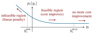
Figure 1: Illustration of Lemma IV.4. See the text for details.

Lemma IV.4.

For all $i\in\{1,\ldots,N\}$, the primal function $p_{i}(y_{i})$ satisfies the following properties:

1. $p_{i}(y_{i})=p_{i}(y^{\textsc{max}}_{i})$ for all $y_{i}\geq y^{\textsc{max}}_{i}$;

2. $p(y_{i})=-My_{i}+q_{i}$ for all $y_{i}\leq y_{i}^{\textsc{min}}$,

with $q_{i}=p_{i}(y^{\textsc{min}}_{i})+My^{\textsc{min}}_{i}$.

Proof.

Let us show (i). Let $\bar{y}\geq y^{\textsc{max}}$ and let $(x^{\textsc{max}},\rho^{\textsc{max}})$ be an optimal solution of problem (6) with $y=y^{\textsc{max}}$. To prove that $p(\bar{y})=p(y^{\textsc{max}})$, we must prove that $(x^{\textsc{max}},\rho^{\textsc{max}})$ is an optimal solution of problem (6) when $y=\bar{y}$. By construction, it holds

$$g(x^{\textsc{max}})\leq y^{\textsc{max}}+\rho^{\textsc{max}}\leq\bar{y}+\rho^{\textsc{max}}$$

thus $(x^{\textsc{max}},\rho^{\textsc{max}})$ is a feasible solution. Suppose that it is not optimal, then there exists $(\tilde{x},\tilde{\rho})$ such that $\tilde{x}\in X$, $\tilde{\rho}\geq 0$, $g(\tilde{x})\leq\bar{y}+\tilde{\rho}$ and

$$f(\tilde{x})+M\tilde{\rho}<f(x^{\textsc{max}})+M\rho^{\textsc{max}},$$

i.e., $(\tilde{x},\tilde{\rho})$ has a lower cost than $(x^{\textsc{max}},\rho^{\textsc{max}})$. However, by (8b) and $\tilde{\rho}\geq 0$ we have

$$g(\tilde{x})\leq\max_{x_{i}\in X_{i}}g_{i}(x_{i})=y^{\textsc{max}}\leq y^{\textsc{max}}+\tilde{\rho}$$

and $(\tilde{x},\tilde{\rho})$ would be a feasible solution for problem (6) with $y=y^{\textsc{max}}$ with a cost lower than $(x^{\textsc{max}},\rho^{\textsc{max}})$, contradicting the assumption that $(x^{\textsc{max}},\rho^{\textsc{max}})$ is optimal.

Now we prove (ii). Let $\bar{y}\leq y^{\textsc{min}}$ and let $(x^{\textsc{min}},\rho^{\textsc{min}})$ be optimal solution of problem (6) with $y=y^{\textsc{min}}$. It holds $p(y^{\textsc{min}})=f(x^{\textsc{min}})+M\rho^{\textsc{min}}$ and $g(x^{\textsc{min}})\leq y^{\textsc{min}}+\rho^{\textsc{min}}$. The goal is to show that

$$p(\bar{y}) =p(y^{\textsc{min}})+M(y^{\textsc{min}}-\bar{y})$$

$$=f(x^{\textsc{min}})+M(\rho^{\textsc{min}}+y^{\textsc{min}}-\bar{y}),$$

i.e. that $(x^{\textsc{min}},\rho^{\textsc{min}}+y^{\textsc{min}}-\bar{y})$ is an optimal solution of problem (6) with $y=\bar{y}$. By using the assumption on $(x^{\textsc{min}},\rho^{\textsc{min}})$ and the fact that $y^{\textsc{min}}-\bar{y}\geq 0$ (by (8a)), we can immediately show feasibility,

$$g(x^{\textsc{min}}) \leq y^{\textsc{min}}+\rho^{\textsc{min}}$$

$$\leq y^{\textsc{min}}+\rho^{\textsc{min}}+y^{\textsc{min}}-\bar{y}.$$

Suppose that $(x^{\textsc{min}},\rho^{\textsc{min}}+y^{\textsc{min}}-\bar{y})$ is not optimal for problem (6) with $y=\bar{y}$. Then, there exists $(\tilde{x},\tilde{\rho})$ such that $\tilde{x}\in X$, $\tilde{\rho}\geq 0$, $g(\tilde{x})\leq\bar{y}+\tilde{\rho}$ and

$$f(\tilde{x})+M\tilde{\rho} <f(x^{\textsc{min}})+M(\tilde{\rho}+y^{\textsc{min}}-\bar{y})$$

$$=p(y^{\textsc{min}})+M(y^{\textsc{min}}-\bar{y}),$$

from which it follows that $f(\tilde{x})+M(\tilde{\rho}+y^{\textsc{min}}-\bar{y})<p(y^{\textsc{min}})$, i.e., the vector $(\tilde{x},\tilde{\rho}+y^{\textsc{min}}-\bar{y})$ has a lower cost than $(x^{\textsc{min}},\rho^{\textsc{min}})$. Moreover, using again $y^{\textsc{min}}-\bar{y}\geq 0$, we obtain

$$g(\tilde{x})\leq\bar{y}+\tilde{\rho}\leq\bar{y}+\tilde{\rho}+y^{\textsc{min}}-\bar{y},$$

from which it follows that $(\tilde{x},\tilde{\rho}+y^{\textsc{min}}-\bar{y})$ is a feasible solution for problem (6) with $y=\bar{y}$ with a cost lower than $(x^{\textsc{min}},\rho^{\textsc{min}})$, contradicting the assumption that $(x^{\textsc{min}},\rho^{\textsc{min}})$ is optimal. ∎

In the forthcoming analysis, the properties of the primal functions highlighted by Lemma IV.4 will be linked to the cost estimation mechanism.

IV-C Uniform convergence of estimated subgradients

In Section III we have seen that, being the cost function unknown, each agent uses a surrogate function in problem (2) in place of the actual objective. Next we provide a sequence of results that show that the estimated subgradients of the primal functions converge to the true ones. This fact will be necessary in the proof of Theorem V.4 to assess that Algorithm 1 can asymptotically find an optimal allocation of problem (5). Similarly to the definition of the primal function (6), let us define $p_{i}^{t}(y_{i})$ as the optimal cost of the subproblem with the surrogate function at time $t$ for a given allocation $y_{i}\in$, i.e.,

$$\begin{split}p_{i}^{t}(y_{i})\triangleq\min_{x_{i},\rho_{i}}\>&\>f_{i}^{t}(x_{i})+M\rho_{i}\\ \textnormal{subj. to}\>&\>g_{i}(x_{i})\leq y_{i}+\rho_{i}\\ &\>x_{i}\in X_{i},\>\>\rho_{i}\geq 0.\end{split}$$ (9)

We will work with the dual problems associated to problems (6) and (9). Let us derive the dual problem associated to (9) (the procedure for problem (6) follows similar arguments). Let us compute the dual function,

$$q_{i}^{t}(\mu_{i}) =\!\operatornamewithlimits{inf\vphantom{p}}_{x_{i}\in X_{i},\>\rho_{i}\geq 0}\!\big{[}f_{i}^{t}(x_{i})+M\rho_{i}+\mu_{i}\big{(}g_{i}(x_{i})-y_{i}-\rho_{i}\big{)}\big{]}$$

$$=\begin{cases}\displaystyle\min_{x_{i}\in X_{i}}\big{[}f_{i}^{t}(x_{i})+\mu_{i}\big{(}g_{i}(x_{i})-y_{i}\big{)}\big{]}&\text{if }\mu_{i}\leq M\\ -\infty&\text{otherwise},\end{cases}$$

where we replaced $\operatornamewithlimits{inf\vphantom{p}}$ with $\min$ since $X_{i}$ is compact. Note that $\mu_{i}\leq M$ is the domain associated to the dual function. The dual problem associated to (9) is

$$\begin{split}\max_{\mu_{i}}\>&\>q_{i}^{t}(\mu_{i})\\ \textnormal{subj. to}\>&\>0\leq\mu\leq M,\end{split}$$ (10)

for all $i\in\{1,\ldots,N\}$. Note that for all $y_{i}\in$ the function $q_{i}^{t}$ is continuous and thus the maximum in (10) exists finite. In a similar way, the dual problem associated to (6) is exactly as problem (10), except that $q_{i}^{t}$ is replaced with the dual function associated to (6), i.e.,

$$q_{i}(\mu_{i})=\begin{cases}\displaystyle\min_{x_{i}\in X_{i}}\big{[}f_{i}(x_{i})+\mu_{i}\big{(}g_{i}(x_{i})-y_{i}\big{)}\big{]}&\text{if }\mu_{i}\leq M\\ -\infty&\text{otherwise}.\end{cases}$$

Lemma IV.5.

Let Assumptions II.1 and II.3 hold. Then, the dual function sequence $\{q_{i}^{t}\}_{t}$ converges to $q_{i}$, uniformly in $\mu_{i}\in D_{i}=\{\mu_{i}:\mu_{i}\leq M\}$ and $y_{i}\in$, where $D_{i}$ is the domain of $q_{i}$ and $q_{i}^{t}$.

Proof.

Since our aim is to prove uniformity with respect to both $\mu$ and $y$, in this proof we denote the functions as $q^{t}(\mu,y)$ and $q(\mu,y)$ to show explicitly the dependence of $q^{t}$ and $q$ on both $\mu$ and $y$. By definition, we have that, for any fixed $\mu\in D$ and $y\in$,

$$q(\mu,y) =\min_{x\in X}\big{(}f(x)+\mu(g(x)-y)\big{)}$$

$$\leq f(x)+\mu(g(x)-y),\hskip 14.22636pt\text{for all }x\in X,$$ (11)

and also

$$q^{t}(\mu,y) =\min_{x\in X}\big{(}f^{t}(x)+\mu(g(x)-y)\big{)}$$

$$\leq f^{t}(x)+\mu(g(x)-y)\hskip 14.22636pt\text{for all }x\in X.$$ (12)

By the uniform convergence of $\{f^{t}\}_{t}$ (cf. Assumption II.3), we have that for all $\varepsilon>0$ there exists $N>0$ such that for all $t\geq N$ it holds

$$f^{t}(x)-f(x)<\varepsilon\hskip 14.22636pt\text{and}\hskip 14.22636ptf(x)-f^{t}(x)<\varepsilon,$$

for all $x\in X$. Subtracting (11) from (12) and using the uniform convergence we obtain, for all $t\geq N$ and for any $\mu\in D$ and $y\in$,

$$q^{t}(\mu,y)-q(\mu,y) \leq f^{t}(x)-f(x)\hskip 19.91684pt\text{for all }x\in X$$

$$<\varepsilon.$$

Similarly, subtracting (12) from (11), we obtain, for all $t\geq N$ and for any $\mu\in D$ and $y\in$,

$$q(\mu,y)-q^{t}(\mu,y)<\varepsilon.$$

Since the previous results do not actually depend on the chosen $\mu$ or $y$, they are uniform in $\mu$ and $y$. Therefore we have proven that for all $\varepsilon>0$ there exists $N\geq 0$ such that $|q^{t}(\mu)-q(\mu)|<\varepsilon$ for all $t\geq N$, uniformly in $y\in$ and $\mu\in D$. ∎

Owing to Lemma IV.2, a subderivative of the time-varying primal function $p_{i}^{t}$ at any $y_{i}\in$ is given by ${p_{i}^{t}}^{\prime}(y_{i})=-\mu_{i}^{t}(y_{i})$, where $\mu_{i}^{t}(y_{i})$ is a maximum of $q_{i}^{t}(\cdot,y_{i})$ (with respect to $\mu_{i}$) in the interval $0\leq\mu_{i}\leq M$. Since there may be several maxima, we now introduce a tie-break rule to make the maximum unique (later it will be formalized specifically for the algorithm, cf. Assumption V.2). In particular, we assume that among all the maxima we always select the smallest one, i.e., we define $\mu_{i}^{t}(y_{i})$ as the function

$$\mu_{i}^{t}(y_{i})\triangleq\min\Big{\{}\mathop{\rm argmax}_{0\leq\mu_{i}\leq M}\>q_{i}^{t}(\mu_{i},y_{i})\Big{\}},$$ (13)

where here we intend the outer minimization as the selection of the smallest number from the set of maxima returned by the $\mathop{\rm argmax}$ operator. With this definition at hand, the subderivative ${p_{i}^{t}}^{\prime}$ defined above is a well-defined function of $y_{i}$. A similar definition holds for the subderivative of $p_{i}(y_{i})$,

$$p_{i}^{\prime}(y_{i})=-\mu_{i}(y_{i})\triangleq-\min\Big{\{}\mathop{\rm argmax}_{0\leq\mu_{i}\leq M}\>q_{i}(\mu_{i},y_{i})\Big{\}}.$$

Lemma IV.6.

Let Assumption II.3 hold. Then, the subderivative function ${p_{i}^{t}}^{\prime}(y_{i})$ converges uniformly to $p_{i}^{\prime}(y_{i})$, i.e. for all $\eta>0$ there exists $N>0$ such that $|{p_{i}^{t}}^{\prime}(y_{i})-p_{i}^{\prime}(y_{i})|<\eta$ for all $t\geq N$ and $y_{i}\in$.

Proof.

To ease the notation, we drop the index $i$. Since ${p^{t}}^{\prime}(y)=-\mu^{t}(y)$, we need to prove that the function $\mu^{t}(y)$ converges uniformly to $\mu(y)$. By definition (13), the function sequence $\{\mu^{t}(y)\}_{t\in{\mathbb{N}}}$ is uniformly bounded in $[0,M]$. Thus we can extract a convergent subsequence $\{\mu^{t_{n}}(y)\}_{n\in{\mathbb{N}}}$ and denote by $\bar{\mu}(y)$ its limit function. Let us first show that the limit function maps each $y$ to a maximum of $q(\mu,y)$ over $\mu\in[0,M]$. For all $y\in$, by optimality of $\mu^{t_{n}}(y)$ for $q^{t_{n}}$ it holds

$$q^{t_{n}}(\mu(y),y)\leq q^{t_{n}}(\mu^{t_{n}}(y),y),\hskip 28.45274pt\forall n\in{\mathbb{N}}.$$

By taking the limit as $n\to\infty$ and by using Lemma IV.5, we obtain for all $y\in$

$$q(\mu(y),y)\leq q(\bar{\mu}(y),y).$$

However, by optimality of $\mu(y)$ for $q$ it also holds $q(\mu(y),y)\geq q(\bar{\mu}(y),y)$ for all $y\in$. Thus, equality follows for all $y$ and therefore

$$\bar{\mu}(y)\in\mathop{\rm argmax}_{\mu\in[0,M]}\>q(\mu,y),\hskip 28.45274pt\forall y\in.$$ (14)

We finally need to show that $\bar{\mu}(y)$ is also the smallest number in $\mathop{\rm argmax}_{\mu\in[0,M]}\>q(\mu,y)$. Let us denote

$$Q^{\star}(y) =\mathop{\rm argmax}_{0\leq\mu\leq M}\>q(\mu,y),$$

$$Q^{t}(y) =\mathop{\rm argmax}_{0\leq\mu\leq M}\>q^{t}(\mu,y).$$

By (13), for all $y\in$ it holds

$$\mu^{t_{n}}(y)\leq\mu,\hskip 28.45274pt\forall\mu\in Q^{t}{t_{n}}(y).$$

By taking the limit as $n$ goes to infinity and by using (14), we obtain for all $y\in$

$$\bar{\mu}(y)\leq\mu,\hskip 28.45274pt\forall\mu\in Q^{\star}(y),$$

and the proof follows. ∎

IV-D Estimated subgradients are epsilon-subgradients

The uniform convergence of the the estimated subgradients is not enough to prove that Algorithm 1 is able to asymptotically recover optimality. However, it turns out that the subgradients of the time-varying primal functions $p_{i}^{t}$ are so-called $\epsilon$-subgradients of the true primal function $p_{i}$. Formally, given a convex function $\varphi(\theta):^{n}\rightarrow$, an $\epsilon$-subgradient of $\varphi$ at some $\theta_{0}\in^{n}$, is a vector $\widetilde{\nabla}_{\epsilon}\varphi(\theta_{0})\in^{n}$ satisfying

$$\varphi(\theta)\geq\varphi(\theta_{0})+\widetilde{\nabla}_{\epsilon}\varphi(\theta_{0})^{\top}(\theta-\theta_{0})-\epsilon,\hskip 28.45274pt\forall\theta\in^{n},$$

In the following important proposition, we prove a central result for the analysis.

Proposition IV.7.

Let Assumptions II.1, II.2 and II.3 hold. Then, there exists a sequence $\{\epsilon_{i}^{t}\}_{t\in{\mathbb{N}}}$ of non-negative scalars such that for all $t\in{\mathbb{N}}$ and $y_{i}\in$ it holds

$$p_{i}(z)\geq p_{i}(y_{i})+(z-y_{i})^{\top}{p_{i}^{t}}^{\prime}(y)-\epsilon_{i}^{t},\hskip 19.91684pt\forall\>z\in.$$ (15)

Moreover, $\displaystyle\operatornamewithlimits{lim\vphantom{p}}_{t\to\infty}\epsilon_{i}^{t}=0$.

Proof.

To ease the notation, we drop the index $i$. We begin by proving that, for each fixed $t$ and $y\in$, there exists a finite number $\epsilon^{t}$ satisfying (15). We will then find an upper bound of $\epsilon^{t}$, independent of $y$, that goes to zero as $t$ goes to infinity, which yields the desired result.

Fix $t\in{\mathbb{N}}$ and $y_{0}\in$. Let us define $\epsilon^{t}(y_{0})$ as the smallest non-negative number satisfying (15) at $y_{0}$, i.e.

$$\begin{split}\epsilon^{t}(y_{0})\!=\!\operatornamewithlimits{inf\vphantom{p}}_{\epsilon}\>&\epsilon\\ \textnormal{subj. to}\>&\epsilon\geq p(y_{0})\!+\!(z\!-\!y_{0}){p^{t}}^{\prime}(y_{0})\!-\!p(z),\>\forall z\in.\end{split}$$ (16)

By definition, $\epsilon^{t}(y_{0})\geq 0$. We must prove that the infimum in (16) is attained at a real number (i.e. that $\epsilon^{t}(y_{0})\neq+\infty$). The optimization problem (16) is in epigraph form and can be equivalently rewritten as

$$\epsilon^{t}(y_{0})=\sup_{z\in}\big{[}p(y_{0})+(z-y_{0}){p^{t}}^{\prime}(y_{0})-p(z)\big{]}.$$ (17a)

Using the properties of the $$\sup \epsilon^{t}(y_{0})$$, we can rewrite as

$$\epsilon^{t}(y_{0})=-\operatornamewithlimits{inf\vphantom{p}}_{z\in}r(z),$$ (17b)

with

$$r(z)=p(z)-z{p^{t}}^{\prime}(y_{0})-p(y_{0})+y_{0}{p^{t}}^{\prime}(y_{0}).$$ (18)

Note that $r(z)$ is also a function of $t$ and $y_{0}$, however we leave these arguments as implicit so as to keep the notation light. We now show that the minimum of $r(z)$ exists, which in turn implies that $\epsilon^{t}(y_{0})\in$. To see this, first note that since $p(z)$ is convex then also $r(z)$ is convex. Let us study the subderivative of $r(z)$. By Lemma IV.4, $p(y)$ is linear for $y\leq y^{\textsc{min}}$ and for $y\geq y^{\textsc{max}}$. Thus, $r(z)$ is differentiable for all $z\in(-\infty,y^{\textsc{min}})\cup(y^{\textsc{max}},+\infty)$. For all $z\leq y^{\textsc{min}}$, it holds

$$r^{\prime}(z)=p^{\prime}(z)-{p^{t}}^{\prime}(y_{0})=-M-{p^{t}}^{\prime}(y_{0})\leq 0,$$

where the last equality follows by Lemma IV.4 and the inequality follows by Lemma IV.3. Analogously, for all $z\geq y^{\textsc{max}}$, it holds

$$r^{\prime}(z)=p^{\prime}(z)-{p^{t}}^{\prime}(y_{0})=-{p^{t}}^{\prime}(y_{0})\geq 0.$$

Thus $r(z)$ is non increasing for $z\leq y^{\textsc{min}}$ and non decreasing for $z\geq y^{\textsc{max}}$. Being the function convex (and thus continuous), there exists a (finite) minimum in the interval $[y^{\textsc{min}},y^{\textsc{max}}]$. i.e.,

$$\min_{z\in}r(z) =\min_{z\in[y^{\textsc{min}},y^{\textsc{max}}]}r(z).$$

Thus, $\epsilon^{t}(y_{0})\in$ since the $\operatornamewithlimits{inf\vphantom{p}}$ in (16) is finite.

Now we proceed to compute a vanishing overestimate of $\epsilon^{t}(y_{0})$. Consider the sequence $\{{p^{t}}^{\prime}(y_{0})\}_{t\in{\mathbb{N}}}$ and fix $\beta>0$. Define $\eta=\beta/|y^{\textsc{min}}-y^{\textsc{max}}|>0$. By Lemma IV.6, there exists $N>0$ such that $|{p^{t}}^{\prime}(y_{0})-p^{\prime}(y_{0})|<\eta$ for all $t\geq N$. To compute the overestimate of $\epsilon^{t}(y_{0})$, we replace $p(z)$ with a convex, piece-wise linear underestimate $p_{y_{0}}^{\textsc{aux}}(z)$, defined as

$$p_{y_{0}}^{\textsc{aux}}(z)=\max\Big{\{} p(y^{\textsc{min}})+M(y^{\textsc{min}}-y),$$

$$p(y_{0})+p^{\prime}(y_{0})(y-y_{0}),\>\>\>p(y^{\textsc{max}})\Big{\}}.$$

The resulting function consists of three pieces. The left-most piece and the right-most piece are obtained by prolonging the two lateral linear pieces of $p(z)$ inside the interval $[y^{\textsc{min}},y^{\textsc{max}}]$, while the central piece is the tangent line crossing $p(z)$ at $y_{0}$. By construction, this function satisfies $p_{y_{0}}^{\textsc{aux}}(z)\leq p(z)$ for all $z\in$. Let us compute the break points, which we denote by $y^{L}$ and $y^{R}$ (see Figure 2). To compute $y^{L}$, we must intersect the first two pieces, i.e.

$$\underbrace{-My^{L}+p(y^{\textsc{min}})+My^{\textsc{min}}}_{\text{left piece}}=\underbrace{p(y_{0})+(y^{L}-y_{0})p^{\prime}(y_{0})}_{\text{central piece}},$$

which results in

$$y^{L}=\frac{p(y^{\textsc{min}})+My^{\textsc{min}}-p(y_{0})+y_{0}p^{\prime}(y_{0})}{p^{\prime}(y_{0})+M}.$$ (19)

Similarly, we can compute $y^{R}$, which is equal to

$$y^{R}=y_{0}+\frac{p(y^{\textsc{max}})-p(y_{0})}{p^{\prime}(y_{0})}.$$ (20)

Notice that the value of $p_{y_{0}}^{\textsc{aux}}(y^{L})$ is equal to $p(y^{\textsc{max}})$.

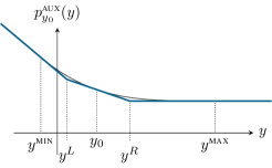
Figure 2: Graphical representation of the surrogate function $p_{y_{0}}^{\textsc{aux}}(z)$ (in blue). The original primal function $p(z)$ is the black curve near the blue one.

Now, similarly to $r(z)$, let us define functions $r^{\textsc{aux},t}(z)$ corresponding to $p^{t}(z)$ for all $t$. Then, we use them to compute the upper bound on $\epsilon^{t}(y_{0})$, in a similar way as in (17a)–(17b). The functions $r^{\textsc{aux},t}(z)$ are defined as

$$r^{\textsc{aux},t}(z)=p_{y_{0}}^{\textsc{aux}}(z)-z{p^{t}}^{\prime}(y_{0})-p(y_{0})+y_{0}{p^{t}}^{\prime}(y_{0}),$$ (21)

for all $t\geq 0$. As before, these functions also depend on $y_{0}$, which is omitted in the notation because it is fixed. It holds $r^{\textsc{aux},t}(z)\leq r(z)$ (since $p_{y_{0}}^{\textsc{aux}}(z)\leq p(z)$). Being $p_{y_{0}}^{\textsc{aux}}(z)$ piece-wise linear with three pieces, then also $r^{\textsc{aux},t}(z)$ is piece-wise linear with three pieces. Similarly to (17b), let us now define the overestimate of $\epsilon^{t}(y_{0})$ as

$$\epsilon^{\textsc{aux},t}(y_{0})\triangleq-\operatornamewithlimits{inf\vphantom{p}}_{z\in}r^{\textsc{aux},t}(z)=-\min_{z\in[y^{L},y^{R}]}r^{\textsc{aux},t}(z),$$

where the equality holds since the function $r^{\textsc{aux},t}(z)$ admits minimum in $[y^{L},y^{R}]$ (by following the same reasoning used for $r(z)$). Since $r^{\textsc{aux},t}(z)\leq r(z)$ for all $z$, the same holds for the minimum of such functions over $[y^{L},y^{R}]$, from which we see that indeed $\epsilon^{\textsc{aux},t}(y_{0})\geq\epsilon^{t}(y_{0})$. Since $r^{\textsc{aux},t}(z)$ is linear in the interval $[y^{L},y^{R}]$, the minimum is attained either at $y^{L}$ or at $y^{R}$:

$$\epsilon^{\textsc{aux},t}(y_{0})=-\min\Big{\{}r^{\textsc{aux},t}(y^{L}),\>\>r^{\textsc{aux},t}(y^{R})\Big{\}}.$$ (22)

Let us compute the value of the function at $y^{L}$ and $y^{R}$, i.e.

$$r^{\textsc{aux},t}(y^{L}) =p_{y_{0}}^{\textsc{aux}}(y^{L})-y^{L}{p^{t}}^{\prime}(y_{0})-p(y_{0})+y_{0}{p^{t}}^{\prime}(y_{0})$$

$$=p(y_{0})+p^{\prime}(y_{0})(y^{L}-y_{0})-y^{L}{p^{t}}^{\prime}(y_{0})$$

$$\hskip 14.22636pt-p(y_{0})+y_{0}{p^{t}}^{\prime}(y_{0})$$

$$=(p^{\prime}(y_{0})-{p^{t}}^{\prime}(y_{0}))(y^{L}-y_{0}),$$

and, similarly,

$$r^{\textsc{aux},t}(y^{R}) =(p^{\prime}(y_{0})-{p^{t}}^{\prime}(y_{0}))(y^{R}-y_{0}),$$

which always have opposite sign since $y^{L}\leq y_{0}\leq y^{R}$. Thus, we can distinguish two cases. If $r^{\textsc{aux},t}(y^{L})\leq 0$, then the minimum in (22) is attained at $r^{\textsc{aux},t}(y^{L})$ and therefore

$$\epsilon^{\textsc{aux},t}(y_{0})=-r^{\textsc{aux},t}(y^{L}) =\underbrace{-(p^{\prime}(y_{0})-{p^{t}}^{\prime}(y_{0}))(y^{L}-y_{0})}_{\geq 0}$$

$$=\underbrace{|p^{\prime}(y_{0})-{p^{t}}^{\prime}(y_{0})|}_{\leq\eta\>\>\forall t\geq N}\underbrace{|y^{L}-y_{0}|}_{\leq|y^{\textsc{min}}-y^{\textsc{max}}|}$$

$$\leq\eta|y^{\textsc{min}}-y^{\textsc{max}}|,\hskip 28.45274pt\forall t\geq N.$$

Likewise, if $r^{\textsc{aux},t}(y^{R})\leq 0$, we obtain

$$\epsilon^{\textsc{aux},t}(y_{0})=-r^{\textsc{aux},t}(y^{R})=-(p^{\prime}(y_{0})-{p^{t}}^{\prime}(y_{0}))(y^{R}-y_{0})$$

$$\leq\eta|y^{\textsc{min}}-y^{\textsc{max}}|,\hskip 14.22636pt\forall t\geq N.$$

In either cases, it holds

$$\epsilon^{t}(y_{0})\leq\epsilon^{\textsc{aux},t}(y_{0})\leq\underbrace{\eta|y^{\textsc{min}}-y^{\textsc{max}}|}_{\beta},\hskip 28.45274pt\forall t\geq N.$$

which is independent of the chosen $y_{0}$. Thus we conclude

$$0\leq\epsilon^{t}\leq\max_{y\in}\epsilon^{t}(y)\leq\max_{y\in}\epsilon^{\textsc{aux},t}(y)\leq\beta,\hskip 14.22636pt\forall t\geq N.$$ (23)

Since $\beta>0$ is arbitrary, it follows that $\displaystyle\operatornamewithlimits{lim\vphantom{p}}_{t\to\infty}\epsilon^{t}=0$. ∎

Note that, in order for Proposition IV.7 to hold, Assumption II.3 is important. Indeed, if Assumption II.3 does not hold, it can be seen that in the previous proof that Lemma IV.6 could not be applied, and thus one could use the fact that $|{p^{t}}^{\prime}(y_{0})-p^{\prime}(y_{0})|<\eta$. As a consequence, (23) would not be valid and it would not be possible to conclude that $\operatornamewithlimits{lim\vphantom{p}}_{t\to\infty}\epsilon^{t}=0$.

V Algorithm Analysis: Convergence Result

In this section, we provide the main theoretical result for the convergence analysis of the distributed algorithm. The line of proof is based on the ideas in [14], however we will need to make the necessary modifications to the analysis since in the local problems (2) we replaced the true cost function with an estimated version. Before introducing the main theoretical result, let us recall the needed results.

V-A Unconstrained Formulation of Master Problem

In order to analyze Algorithm 1, we proceed to perform a graph-induced reformulation of the master problem (5) that makes it amenable to distributed computation. Formally, consider the communication graph $\mathcal{G}=(V,\mathcal{E})$. For all edges $(i,j)\in\mathcal{E}$, let $z_{ij}\in$ be a vector associated to the edge $(i,j)$ and denote by $z\in^{|\mathcal{E}|}$ the vector stacking all $z_{ij}$. Consider the change of coordinates for problem (5) defined through the following linear mapping

$$y_{i}=\sum_{j\in\mathcal{N}_{i}}\!(z_{ij}-z_{ji})+\frac{b}{N},\hskip 14.22636pt\forall\>i\in\{1,\ldots,N\}.$$ (24)

The main point in introducing these new variables is that they implicitly encode the constraint of the master problem, i.e.,

$$\sum_{i=1}^{N}y_{i}=\sum_{i=1}^{N}\sum_{j\in\mathcal{N}_{i}}\!(z_{ij}-z_{ji})+b=b,$$

which follows by the assumption that $\mathcal{G}$ is undirected. Let us apply this change of coordinates to problem (5). Formally, for all $i\in\{1,\ldots,N\}$, define the functions

$$\tilde{p}_{i}\big{(}\{z_{ij},z_{ji}\}_{j\in\mathcal{N}_{i}}\big{)}\triangleq p_{i}\bigg{[}\sum_{j\in\mathcal{N}_{i}}\!(z_{ij}-z_{ji})+\frac{b}{N}\bigg{]},\hskip 5.69046ptz\in^{|\mathcal{E}|}.$$

In the next lemma we recall the formal equivalence of the master problem with its unconstrained version.

Lemma V.1 ([14, Corollary 4.2]).

Problem (5) is equivalent to the unconstrained optimization problem

$$\min_{z\in|\mathcal{E}|}\>\sum_{i=1}^{N}\tilde{p}_{i}\big{(}\{z_{ij},z_{ji}\}_{j\in\mathcal{N}_{i}}\big{)},$$ (25)

in the sense that (i) the optimal costs are equal, and (ii) if $\{z_{(ij)}^{\star}\}_{(i,j)\in\mathcal{E}}$ is optimal for (25), then $y_{i}^{\star}=(z_{ij}^{\star}-z_{ji}^{\star})+b/N$ for all $i\in\{1,\ldots,N\}$ is an optimal solution of (5). $\square$

In the following, we denote the cost function of (25) as $\tilde{p}(z)=\sum_{i=1}^{N}\tilde{p}_{i}\big{(}\{z_{ij},z_{ji}\}_{j\in\mathcal{N}_{i}}\big{)}$.

V-B Convergence Theorem

We are now ready to formulate the main theoretical result. We formalize the assumption on the tie-break rule, stating that among all the Lagrange multipliers of problem (2) we choose the smallest one.

Assumption V.2 (Tie-break rule).

At each iteration $t\geq 0$, each agent $i\in\{1,\ldots,N\}$ selects $\mu_{i}^{t}$ as the smallest Lagrange multiplier of problem (2).

As regards the step-size, we make the following standard assumption.

Assumption V.3.

The step-size sequence $\{\alpha^{t}\}_{t\geq 0}$, with each $\alpha^{t}\geq 0$, satisfies $\sum_{t=0}^{\infty}\alpha^{t}\!=\!\infty$ and $\sum_{t=0}^{\infty}(\alpha^{t})^{2}\!<\!\infty$. $\square$

The convergence theorem is reported next.

Theorem V.4.

Let Assumptions II.1, II.2, II.3, V.3 and V.2 hold. Then, assuming the allocation vectors $y_{i}^{0}$ are initialized such that $\sum_{i=1}^{N}y_{i}^{0}=b$, for a sufficiently large $M>0$ the sequences $\{x_{i}^{t}\}_{t\geq 0}$ and $\{y_{i}^{t}\}_{t\geq 0}$ generated by Algorithm 1 for all $i\in\{1,\ldots,N\}$ are such that

1. the sequence $\{(y_{1}^{t},\ldots\,y_{N}^{t})\}_{t\geq 0}$ converges to an optimal solution of problem (5);

2. $\operatornamewithlimits{lim\vphantom{p}}_{t\to\infty}\sum_{i=1}^{N}f_{i}^{t}(x_{i}^{t})+M\rho_{i}^{t}=f^{\star}$, where $f^{\star}$ is the optimal cost of (1);

3. every limit point of $\{(x_{1}^{t},\ldots\,x_{N}^{t})\}_{t\geq 0}$ is an optimal solution of (1).

Proof.

By Lemma IV.1 and Lemma V.1, problem (25) has the same optimal cost as problem (1). Recall that $p_{i}^{t}(y_{i})$ denotes the optimal cost of problem (2) for all $i\in\{1,\ldots,N\}$ and $t\geq 0$. Let us consider a subgradient method applied to problem (25). Instead of the standard subgradient method, we replace the subgradients of $\tilde{p}_{i}\big{(}\{z_{ij}^{t},z_{ji}^{t}\}_{j\in\mathcal{N}_{i}}\big{)}$ with a subgradient of $\tilde{p}_{i}^{t}\big{(}\{z_{ij}^{t},z_{ji}^{t}\}_{j\in\mathcal{N}_{i}}\big{)}\triangleq p_{i}^{t}[\sum_{j\in\mathcal{N}_{i}}\!(z_{ij}^{t}-z_{ji}^{t})]$ and therefore consider the update

$$z_{ij}^{t+1} =z_{ij}^{t}-\alpha^{t}{\tilde{p}_{i}^{t}}\>\!^{\prime}\big{(}\{z_{ij}^{t},z_{ji}^{t}\}_{j\in\mathcal{N}_{i}}\big{)}\hskip 14.22636pt\forall(i,j)\in\mathcal{E},$$ (26)

initialized at some $z^{0}\in^{|\mathcal{E}|}$. As we will see in a moment, the update (26) is in fact an $\epsilon$-subgradient method applied to problem (25). By Lemma IV.2, the subderivatives of $p_{i}^{t}$ at $\sum_{j\in\mathcal{N}_{i}}(z_{ij}^{t}-z_{ji}^{t})$ are equal to

$${p_{i}^{t}}^{\prime}\bigg{[}\sum_{j\in\mathcal{N}_{i}}(z_{ij}^{t}-z_{ji}^{t})\bigg{]}=-\mu_{i}^{t},$$

where $\mu_{i}^{t}$ is a Lagrange multiplier of problem (9) (with $y_{i}=\sum_{j\in\mathcal{N}_{i}}(z_{ij}-z_{ji})$) associated to the constraint $g_{i}(x_{i})\leq y_{i}+\rho_{i}$. As shown in [14], using the change of coordinates (24) we can show that the subderivatives of $\tilde{p}_{i}^{t}$ are equal to

$${\tilde{p}_{i}^{t}}\>\!^{\prime}\big{(}\{z_{ij}^{t},z_{ji}^{t}\}_{j\in\mathcal{N}_{i}}\big{)}=\mu_{j}^{t}-\mu_{i}^{t},\hskip 28.45274pt\forall(i,j)\in\mathcal{E},$$

from which it follows that the update (26) can be rewritten as

$$z_{ij}^{t+1} =z_{ij}^{t}+\alpha^{t}(\mu_{j}^{t}-\mu_{i}^{t}),\hskip 28.45274pt\forall(i,j)\in\mathcal{E}.$$ (27)

By Proposition IV.7, together with Assumption V.2 and Lemma IV.6, we finally see that the update (27) is an $\epsilon$-subgradient method applied to problem (25), with $\epsilon^{t}=\displaystyle\max_{i}\epsilon_{i}^{t}$ going to $0$ as $t$ goes to $\infty$. Thus, by following the arguments of [25, Section 3.3] and by also using the boundedness of the subderivatives (Lemma IV.3) and Assumption V.3, we conclude that the sequence $\{z^{t}\}_{t\geq 0}$ generated by (27) converges to an optimal solution $z^{\star}$ of problem (25).

Let us rewrite the update (27) in terms of $y$ by using the change of coordinate (24),

$$y_{i}^{t+1} =\sum_{i=1}^{N}\bigg{[}\sum_{j\in\mathcal{N}_{i}}(z_{ij}^{t}-z_{ji}^{t})+b/N\bigg{]}$$

$$=y_{i}^{t}+\alpha^{t}\sum_{j\in\mathcal{N}_{i}^{t}}\big{(}\mu_{i}^{t}-\mu_{j}^{t}\big{)},$$ (28)

where we also used the fact that the graph is undirected and that $\sum_{i=1}^{N}y_{i}^{t}=b$ for all $t\geq 0$ (by induction). Note that (28) is exactly the algorithm update (3). Moreover, the sequence $\{y^{t}\}$ is correctly initialized in Algorithm 1, since by (28) it must hold $\sum_{i=1}^{N}y_{i}^{0}=b$. Thus, we conclude that the sequence $\{y^{t}\}_{t\geq 0}$ converges to $y^{\star}$, with components equal to

$$y_{i}^{\star}=\sum_{j\in\mathcal{N}_{i}}(z_{ij}^{\star}-z_{ji}^{\star})+b/N,\hskip 28.45274pti\in\{1,\ldots,N\}.$$

Thus, point (i) follows by Lemma V.1. We have thus shown that the sequence $\{y^{t}\}_{t\geq 0}$ generated by Algorithm 1 converges to an optimal solution of problem (5).

Having proven (i), point (ii) can be proven with the same arguments as in [14, Theorem 2.5 (i)].

To prove (iii), Consider the primal sequence $\{(x_{1}^{t},\ldots,x_{N}^{t},\rho_{1}^{t},\ldots,\rho_{N}^{t})\}_{t\geq 0}$ generated by the Algorithm 1. By summing over $i\in\{1,\ldots,N\}$ the inequality $g_{i}(x_{i}^{t})\leq y_{i}^{t}+\rho_{i}^{t}\mathds{1}$ (which holds by construction), it holds

$$\sum_{i=1}^{N}g_{i}(x_{i}^{t})\leq\sum_{i=1}^{N}y_{i}^{t}+\sum_{i=1}^{N}\rho_{i}^{t}\mathds{1}=\sum_{i=1}^{N}\rho_{i}^{t}\mathds{1}.$$ (29)

Define $\rho^{t}=\sum_{i=1}^{N}\rho_{i}^{t}$. By construction, the sequence $\{(x_{1}^{t},\ldots,x_{N}^{t},\rho^{t})\}_{t\geq 0}$ is bounded (as a consequence of point (ii) and continuity of the functions $f_{i}^{t}(x_{i})+M\rho_{i}$), so that there exists a sub-sequence of indices $\{t_{h}\}_{h\geq 0}\subseteq\{t\}_{t\geq 0}$ such that the sequence $\{(x_{1}^{t_{n}},\ldots,x_{N}^{t_{h}},\rho^{t_{h}})\}_{h\geq 0}$ converges. Denote the limit point of such sequence as $(\bar{x}_{1},\ldots,\bar{x}_{N},\bar{\rho})$. From point (ii) of the theorem and by using the uniform convergence of the objective functions (cf. Assumption II.3), it follows that

$$\sum_{i=1}^{N}f_{i}(\bar{x}_{i})+M\bar{\rho}=f^{\star}.$$

By Lemma IV.1, it must hold $\bar{\rho}=0$. As the functions $g_{i}$ are continuous, by taking the limit in (29) as $h\to\infty$, with $t=t_{h}$, it holds $\sum_{i=1}^{N}g_{i}(\bar{x_{i}})\leq\bar{\rho}\mathds{1}=\mathbf{0}$. Therefore, the point $(\bar{x}_{1},\ldots,\bar{x}_{N})$ is an optimal solution of problem (1). ∎

VI Numerical Computations

In this section, we show numerical computations to corroborate the theoretical results. To estimate the cost functions, we consider a method similar to the one in [17], without all the machinery to guarantee smoothness and strong convexity.

Formally, fix an agent $i$ and consider $K\in{\mathbb{N}}$ samples $z_{i}^{1},\ldots,z_{i}^{K}\in X_{i}$. To build the estimated function, we let the agent compute $\gamma_{1},\ldots,\gamma_{K}\in^{n_{i}}$ by solving the feasibility problem

$$\begin{split}\text{find}\>&\>\gamma^{1},\ldots,\gamma^{K}\\ \textnormal{subj. to}\>&\>f_{i}(z_{i}^{h})\!+\!(z_{i}^{\ell}\!-\!z_{i}^{h})^{\top}\gamma^{h}\leq f_{i}(z_{i}^{\ell}),\\ &\hskip 56.9055pt\text{for all }h,\ell=1,\ldots,K,\>h\neq\ell\end{split}$$ (30)

The purpose of problem (30) is to compute the slope of the linear pieces that build up the estimation of $f_{i}$ and has $K$ variables and $K(K-1)$ convexity constraints. With the solutions $(\gamma^{1},\ldots,\gamma^{K})$ at hand, the oracle returns the estimated functions in the following form:

$$f_{i}^{K}(x)=\max_{k\in\{1,\ldots,K\}}\big{\{}f_{i}(z_{i}^{k})+(x-z_{i}^{k})^{\top}\gamma^{k}\big{\}},$$ (31)

for all $i\in\{1,\ldots,N\}$. Note that $f_{i}^{K}(\cdot)$ is a piece-wise linear function. Moreover, $f_{i}^{K}$ is the pointwise maximum of a finite number of affine functions, its epigraph is a non-empty polyhedron, and hence $f_{i}^{K}$ is convex, closed and proper (see Theorem 1 in [26]).

At each iteration, each agent $i$ collects a new sample of the domain. Initially the samples are independent and identically distributed in the whole domain. As more points are added to the model, we start to reduce the space where sampling new points into balls centered in the current approximated solution. In fact, restricting the sampling space, force the model to refine the surrogate function in those area containing the approximated solution. We experimentally tested that, thanks to the latter expedient, it is possible to reduce the number of samples to keep in the memory. In fact, if the cost function becomes interesting only near the minimum, from a certain point on, estimating the part of the function far from the minimum becomes irrelevant, and all samples far from the minimum can be canceled. By following this intuition, together with the fact that the sample space is shrinking more and more around the potential solution, the samples collected further away in terms of time can be removed from the model. This relieves the function estimation, whose complexity is dependent on the number of points used.

We consider a network of $N=10$ agents in a 3-dimensional domain. We generate a random Erdős-Rényi graph with edge probability $0.2$. We consider quadratic local functions $f_{i}$ and linear local constraints $g_{i}$. Figure 3 shows the evolution of the algorithm in terms of cost error $|f^{\star}-\sum_{i=1}^{N}f_{i}(x_{i}^{t})|$. Despite the use of surrogate cost functions, the objective value converges to the optimal cost of the original problem with known cost function, as we expected from the theoretical results.

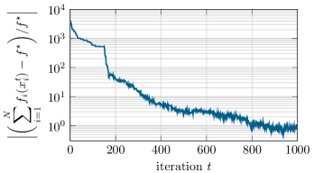
Figure 3: Evolution of the cost error in the numerical example.

VII Conclusions

In this paper, we considered a challenging distributed optimization scenario arising in several control problems of interest. We focused on constraint-coupled optimization problems with unknown cost functions to be learned and we proposed a distributed optimization algorithm that only uses estimated versions of the cost functions. We performed a thorough exploration of the primal decomposition approach, by which concluded that the distributed algorithm can be recast as an epsilon-subgradient that asymptotically recovers consistency and provides an optimal solution to the original problem.

-A Proof of Lemma IV.2

Fix an agent $i$. By Lemma IV.2, it holds $p_{i}^{\prime}(y_{i})=-\mu_{i}(y_{i})$, where $\mu_{i}(y_{i})$ is a Lagrange multiplier of problem (6) associated to the constraint $g_{i}(x_{i})\leq y_{i}+\rho_{i}$. Let us derive the dual function,

$$q_{i}(\mu_{i}) =\operatornamewithlimits{inf\vphantom{p}}_{x_{i}\in X_{i},\>\rho_{i}\geq 0}\Big{(}f_{i}(x_{i})+M\rho_{i}+\mu_{i}(g_{i}(x_{i})-y_{i}-\rho_{i})\Big{)}$$

$$=\begin{cases}\displaystyle\min_{x_{i}\in X_{i}}\>\Big{(}f_{i}(x_{i})+\mu_{i}(g_{i}(x_{i})-y_{i})\Big{)}&\hskip 8.5359pt\text{if }\mu_{i}\leq M,\\ -\infty&\hskip 8.5359pt\text{otherwise}.\end{cases}$$

Thus, the dual problem reads

$$\max_{0\leq\mu_{i}\leq M}\> \>q_{i}(\mu_{i}),$$

from which we see that any optimal solution satisfies $0\leq\mu_{i}(y_{i})\leq M$. Therefore, it follows that $-M\leq p_{i}^{\prime}(y_{i})\leq 0$. $\square$

References

• [1] F. Bullo, Lectures on network systems.   Kindle Direct Publishing, 2019.
• [2] F. Sasso, A. Coluccia, and G. Notarstefano, “Interaction-based distributed learning in cyber-physical and social networks,” IEEE Transactions on Automatic Control, vol. 65, no. 1, pp. 223–236, 2019.
• [3] M. G. Rabbat and R. D. Nowak, “Quantized incremental algorithms for distributed optimization,” IEEE Journal on Selected Areas in Communications, vol. 23, no. 4, pp. 798–808, 2005.
• [4] F. Bullo, J. Cortes, and S. Martinez, Distributed control of robotic networks: a mathematical approach to motion coordination algorithms.   Princeton University Press, 2009, vol. 27.
• [5] J. Cortés and M. Egerstedt, “Coordinated control of multi-robot systems: A survey,” SICE Journal of Control, Measurement, and System Integration, vol. 10, no. 6, pp. 495–503, 2017.
• [6] A. Nedic and A. Ozdaglar, “Distributed subgradient methods for multi-agent optimization,” IEEE Transactions on Automatic Control, vol. 54, no. 1, pp. 48–61, 2009.
• [7] P. Di Lorenzo and G. Scutari, “Next: In-network nonconvex optimization,” IEEE Transactions on Signal and Information Processing over Networks, vol. 2, no. 2, pp. 120–136, 2016.
• [8] D. Varagnolo, F. Zanella, A. Cenedese, G. Pillonetto, and L. Schenato, “Newton-raphson consensus for distributed convex optimization,” IEEE Transactions on Automatic Control, vol. 61, no. 4, pp. 994–1009, 2015.
• [9] D. Mateos-Núnez and J. Cortés, “Distributed saddle-point subgradient algorithms with Laplacian averaging,” IEEE Transactions on Automatic Control, vol. 62, no. 6, pp. 2720–2735, 2017.
• [10] G. Notarstefano, I. Notarnicola, and A. Camisa, “Distributed optimization for smart cyber-physical networks,” Foundations and Trends® in Systems and Control, vol. 7, no. 3, pp. 253–383, 2019.
• [11] D. P. Palomar and M. Chiang, “A tutorial on decomposition methods for network utility maximization,” IEEE Journal on Selected Areas in Communications, vol. 24, no. 8, pp. 1439–1451, 2006.
• [12] P. Giselsson, M. D. Doan, T. Keviczky, B. De Schutter, and A. Rantzer, “Accelerated gradient methods and dual decomposition in distributed model predictive control,” Automatica, vol. 49, no. 3, pp. 829–833, 2013.
• [13] I. Notarnicola and G. Notarstefano, “Constraint-coupled distributed optimization: a relaxation and duality approach,” IEEE Transactions on Control of Network Systems, vol. 7, no. 1, pp. 483–492, 2019.
• [14] A. Camisa, F. Farina, I. Notarnicola, and G. Notarstefano, “Distributed constraint-coupled optimization via primal decomposition over random time-varying graphs,” arXiv preprint arXiv:2010.14489, 2020.
• [15] Q. T. Dinh, I. Necoara, and M. Diehl, “A dual decomposition algorithm for separable nonconvex optimization using the penalty function framework,” in 52nd IEEE Conference on Decision and Control.   IEEE, 2013, pp. 2372–2377.
• [16] Q. Tran-Dinh, I. Necoara, and M. Diehl, “Fast inexact decomposition algorithms for large-scale separable convex optimization,” Optimization, vol. 65, no. 2, pp. 325–356, 2016.
• [17] A. Simonetto, “Smooth strongly convex regression,” arXiv preprint arXiv:2003.00771, 2020.
• [18] C. K. Williams and C. E. Rasmussen, Gaussian processes for machine learning.   MIT press Cambridge, MA, 2006, vol. 2, no. 3.
• [19] E. Schulz, M. Speekenbrink, and A. Krause, “A tutorial on gaussian process regression: Modelling, exploring, and exploiting functions,” Journal of Mathematical Psychology, vol. 85, pp. 1–16, 2018.
• [20] M. Todescato, A. Carron, R. Carli, G. Pillonetto, and L. Schenato, “Multi-robots gaussian estimation and coverage control: From client–server to peer-to-peer architectures,” Automatica, vol. 80, pp. 284–294, 2017.
• [21] A. Benevento, M. Santos, G. Notarstefano, K. Paynabar, M. Bloch, and M. Egerstedt, “Multi-robot coordination for estimation and coverage of unknown spatial fields,” in 2020 IEEE International Conference on Robotics and Automation (ICRA).   IEEE, 2020, pp. 7740–7746.
• [22] A. Camisa, F. Farina, I. Notarnicola, and G. Notarstefano, “Distributed constraint-coupled optimization over random time-varying graphs via primal decomposition and block subgradient approaches,” in 2019 IEEE 58th Conference on Decision and Control (CDC).   IEEE, 2019, pp. 6374–6379.
• [23] G. J. Silverman, “Primal decomposition of mathematical programs by resource allocation: I–basic theory and a direction-finding procedure,” Operations Research, vol. 20, no. 1, pp. 58–74, 1972.
• [24] D. P. Bertsekas, Nonlinear programming.   Athena Scientific, 1999.
• [25] D. P. Bertsekas and A. Scientific, Convex optimization algorithms.   Athena Scientific Belmont, 2015.
• [26] A. B. Taylor, J. M. Hendrickx, and F. Glineur, “Smooth strongly convex interpolation and exact worst-case performance of first-order methods,” Mathematical Programming, vol. 161, no. 1-2, pp. 307–345, 2017.