Modeling the dynamics of language change: logistic regression, Piotrowski’s law, and a handful of examples in Polish

Abstract

The study discusses modeling diachronic processes by logistic regression. The phenomenon of nonlinear changes in language was first observed by Raimund Piotrowski (hence labelled as Piotrowski’s law), even if actual linguistic evidence often speaks against using the notion of a “law” in this context. In our study, we apply logistic regression models to 9 changes which occurred between 15^th and 18^th century in the Polish language. The attested course of the majority of these changes closely follow the expected values, which proves that the language change might indeed resemble a nonlinear phase change scenario. We also extend the original Piotrowski’s approach by proposing polynomial logistic regression for these cases which can hardly be described by its standard version. Also, we propose to consider individual language change cases jointly, in order to inspect their possible collinearity or, more likely, their different dynamics in the function of time. Last but not least, we evaluate our results by testing the influence of the subcorpus size on the model’s goodness-of-fit.

1 Introduction

One can hardly imagine a different picture of a language change than that it starts among a small (possibly sociologically or spatially restricted) group of speakers, gradually gaining more and more users over time, even if conservative speakers somewhat retard the change. After the first period of a slow dissemination, however, the change accelerates until the newly introduced form is broadly accepted by language users. The recessive form gradually becomes rare, and finally dies out, partly because its adherents die as well. Certainly, it takes time for the change to be completed.

The above scenario describes many other natural phenomena. Similar processes can be found in biology, demography or epidemics. To give an example: assume a cup of milk, into which a drop of yogurt (i.e. Lactobacillus delbrueckii ssp. bulgaricus) is added. At the beginning, the population of bacteria is small, yet increasing. Then the growth of the population accelerates rapidly, due to binary fission of the bacteria. However, at a certain point there is no more room (or food, to be precise) for new bacteria to fission, therefore the increase slows down and the population stabilizes. The same scenario applies to the dynamics of an epidemic. In such a case, the analogy with language change is even more striking, since people tend to “infect” other members of the linguistic community with innovative forms. The more users adopt the innovation, the higher the probability of the “disease” to further disseminate, i.e. a speaker will reproduce an innovative form which she/he heard recently or, even more typically, a child will reproduce a form it encounters. Needless to say, significant differences between biology and language still exist: while a virus infection might be caused by one single contact, it is fairly naïve to assume that language change might be caused by one attestation. Rather, a longer exposure to the innovative form is needed for a change to happen. We can assume with a high level of confidence that when a newly introduced form becomes predominant, the chance of adopting it by a conservative speaker increases as well.

On theoretical grounds, a language change can follow one of two main scenarios. Firstly, it can be an innovation that affects a language system without displacing any already-existing forms. In general, vocabulary growth falls into this category (e.g. the emergence of the word nettiquette in the system does not force the word etiquette to withdraw). The second scenario takes place when a new form inevitably replaces an old one, e.g. the degree to which the form burned (the past form of the verb to burn) spreads in English, by definition equals to the withdrawal of the irregular form burnt. In mathematical terms, the probability of finding a new form and an old form (denoted as n and o, respectively) in such a scenario is $p(n)=1-p(o)$, which also implies that $p(o)=1-p(n)$. Consequently, the joint frequency of the two forms might remain constant over the centuries, while their mutual proportions usually vary to a significant degree.

The present study is aimed at measuring the above proportions, in order to model the transition from the recessive to the innovative form. A general framework for modeling such a transition will be logistic regression, which in the context of historical linguistics is often referred to as Piotrowski’s law (Piotrowskaja and Piotrowski, 1974; Best, 1983; Leopold, 2005).

The study will examine to which extent a theoretical model can explain actual language changes. The examples will be drawn from the Polish language. Namely, a few changes that are reported in handbooks of the history of Polish to have taken place between the 15^th and 18^th centuries, will be used to validate the theoretical models. Even if the changes in question have been already observed by diachronic linguistics, the present paper will rely on substantially broader empirical material drawn from a diachronic corpus of Polish of ca. 12 million words, covering the time span of a few centuries. Unlike anecdotal evidence based on single attestations known to the linguists, a corpus-driven approach allows for harvesting the material on an unprecedented scale, which, in turn, leads to fairly precise comparisons of the goodness-of-fit between the observed data points and the expected values predicted by a model.

More importantly, in our approach we will compare the dynamics of different changes by analyzing them side by side, which to our best knowledge has not been proposed before. In the previous studies, the changes were analyzed as isolated phenomena, with a tacit assumption that their trajectories must have been similar. We take into account that an alternative hypothesis is also feasible, namely that the dynamics of particular language changes might differ. Specifically, we believe that there exist innovative forms that introduce the change within decades, whereas some other need centuries to replace their recessive counterparts.

2 The changes

The written record of Polish starts relatively late compared to most languages of Western Europe. Leaving aside single attestations of Polish words in Latin documents, the earliest written texts in Polish date from the end of the 14^th century. The number of texts grows significantly throughout the 15^th century, nevertheless it can still be considered scarce. The number of extant texts continues to be low also in the first half of the 16^th century, and after this point the volume of texts rapidly accelerates. The increase will soon follow an exponential pattern.

It is a claim broadly accepted that Polish saw some major changes at the beginning of the 16^th century (Klemensiewicz, 1965). Not only were a few grammatical categories swept out of the language system (the aorist tense being an example, as well as the dual number), but also the vocabulary was considerably expanded, let alone stabilization of orthography. Also, roughly at the same time a major literary figure and a prolific author Mikołaj Rej (1505–1569) wrote several works that were to commence a tradition of Polish high-brow literature, which always played an important role in forming the standard variant of the Polish language. Next moment in history of a similar impact on Polish is usually associated with the last phase of the Enlightenment at the turn of the 18^th century. No wonder, then, that the time span between the half of the 16^th and the third quarter of the 18^th century is commonly considered a distinct epoch of Polish, usually labelled as the Middle Polish period (Klemensiewicz, 1965).

In the present study, we focus on a few changes that took place in Middle Polish. These are as follows:

• abo > albo (‘or’)

• wszytek > wszystek (‘all’, ‘entire’)

• inszy > inny (‘another’, ‘other’)

• barzo > bardzo (‘very’)

• na- > naj- (a prefix, marker of the superlative)

• -bych > -bym (marker of subjunctive 1^st singular)

• -bychmy > -byśmy (marker of subjunctive 1^st plural)

• -ir- > -er-

• więtszy > większy (‘larger’, ‘bigger’, comparative)

Arguably, the above changes are of very diverse nature. While -ir- > -er- is a purely phonetic and regular change, the first five items on the list are isolated changes. In the transition of barzo > bardzo the fricative /z/ is changed to the affricate /dz/. Both wszytek > wszystek and inszy > inny are isolated changes occurring in a single word, whereas na- > naj- is a modification of a morpheme that was not caused by a regular sound change. The transition -bych > -bym, as well as -bychmy > -byśmy, is a morphological change with one morpheme replacing another ([x] > [m] and [xmi] > [smi]).

3 The so-called Piotrowski’s law

As already mentioned, the replacement of the recessive form by its innovative counterpart is never immediate. Just the contrary, the two forms coexist for some time. In probabilistic terms, it can be said that the probability of finding the innovative form in the period before the change is roughly 0 (tending to 0). In turn, when the change is completed, the innovative form occurs with a probability of 1 (or tending to 1). In the transition period, however, the proportion of the two forms as a function of time follow an “s”-shaped curve (see e.g. Figs. 1–6), which can be described by a non-linear mathematical model. This process has been originally observed by Rajmund Piotrowski (1974), and elaborated by Gabriel Altmann (1983; Köhler and Tuzzi, 2015):

$$p(t)=\frac{1}{1+a\times e^{-rt}}$$

where a is an arbitrary parameter – a positive number by which the trajectory of the function is shifted on the time axis; t = 0 when the proportion between recessive and innovative forms is 1:1; and r is a parameter which is to be adjusted to the empirical data. Traditionally, e denotes the Euler’s number. The parameter r allows for shaping the curve, that is to stretch it to a desired extent.

Interestingly, the same model can describe two different linguistic phenomena. Not only is it applicable to language changes, but also to orthographic variation (Basu, 2016) and most notably, to lexical borrowings: loanwords from a certain donor percolate to the host language in a timespan of the donor’s cultural attractiveness. The number of loanwords originating from one language-borrower in the host language is initially small, and then it raises gradually until it reaches a point of stabilization, with virtually no new loanwords, when the donor language is no more fashionable or the contacts are less intensive than before (Best, 2013; Stachowski, 2016; Gnatchuk, 2015).

For anyone familiar with statistic methodology it is rather obvious that the “s”-shaped curve is usually associated with logistic regression models. And indeed, it has been observed (Vulanović, 2007; Vulanović and Baayen, 2007; Köhler and Tuzzi, 2015) that the model suggested by Altman and Piotrowski is, in fact, a variant of the well-known logistic regression model:

$$p(X)=\frac{1}{1+e^{-(\beta_{0}+\beta_{1}X)}}$$

where $\beta_{0}$ and $\beta_{1}$ determine the logistic intercept and slope. The major advantage of using the logistic regression over the original Piotrowski’s model is that the former allows for a direct comparison of two variables – the proportion of innovative form against the year – whereas in the original approach, the variable t (for time) remains relative and uses a somewhat vague numeric scale, e.g. from -6 to 6. Another reason that makes logistic regression a better choice over the original Piotrowski’s equation is its simpler form which requires less parameters. In practical terms, logistic regression is a time-proven solution, as it is routinely used in countless applications in quantitative linguistic and beyond, and it can be performed using out-of-the-shelf statistical software.

Last but not least, logistic regression models are able to account for data imbalance. Given the almost-exponential growth of literary production over the centuries, one can safely assume that the number of attestations retrieved from medieval works will be significantly scarcer than the evidence from the later periods. While logistic regression is fairly resistant to data imbalance, the extreme unevenness of diachronic corpora might prove problematic. The issue might or might not be important (it has never been raised in previous studies, let alone systematic testing), therefore we will report the results for both standard logistic regression models, and their weighted variants. As prior weights, we use the sum of innovative and recessive forms’ attestations in each time span.

4 Corpus and text preprocessing

The study is based on a tailored diachronic corpus of Polish, which covers a period between 1380 and 1850 and comprises ca. 12 million running words in 790 texts (Górski et al., 2019). While the size of the corpus was essential for the purpose of the current study, our corpus was compiled with an eye on its bulk rather than balance. Understandably, in the case of early historical data the number of available texts is by definition limited, moreover the entire textual output of the Polish Middle Ages consists of religious and legal texts. A simple rule applies here: the older the time period to be covered by a corpus, the bigger the expected bias. Therefore, we were guided by the principle that any text extant was included in the corpus, as long as it was available in electronic format.

Similarly, the distribution of the texts over time was uneven: in terms of running words, some 5% of the corpus (or 0.72 million running words) covers the time until 1550. In turn, the years 1550–1600 make up 12%, the 17^th century – 47%, the 18^th century – 27%, and finally 9% of the corpus covers the years 1800–1850. We decided not to diminish the disproportionately large subcorpus of the 17^th century. However: since our study is aimed at examining the proportion between two forms – a recessive one and an innovative one – and not at actual word occurrences over time, uneven temporal coverage of the corpus should not mislead a logistic regression model to a significant extent. Also, it can be seen that the two outermost periods (before 1550 and after 1800) are significantly smaller than the others. These periods, however, in most cases serve as a background, or the time when either the change has not started yet, or it has been already completed. Still, one has to bear in mind that the corpus includes the entire known textual output of the Middle Ages, and nearly so for the first half of the 16^th century.

A potentially severe issue is an uneven representation of certain text genres in particular time periods, e.g. the overrepresentation of religious treatises in the late Middle Ages, as well as the overrepresentation of belles lettres in the 19^th century. Regardless of several reasons of such a textual/cultural bias in any diachronic corpus, we hardly believe it can ever be reliably corrected for. However, since different genres do not affect morphology as they affect lexis, we assume that grammatical language changes will be reliably reflected in our corpus anyway. We did not make use of POS tagging of the texts, and again for the same reason. A bulk of research shows that the accuracy of tagging for historical texts is substantially lower compared to modern ones; the same rule is probably even more valid in the case of under-resourced languages, such as Polish. Luckily enough, however, the language phenomena to be discussed in the present study can be easily accessed via plain text queries, in some cases (e.g., -ir- > -ier-) followed by manual final selection.

Yet another caveat needs to be introduced. The texts collected in the corpus might be, and usually are, of different size. We did not attempt at trimming long texts, though. Firstly, it is widely agreed upon in corpus linguistics that the texts should be included as a whole rather than sampled, since each part of a text has its own peculiarities (Meyer, 2002). Secondly, with the scarcity of historical data, it would be improvident to let large amounts of already-acquired data be wasted. At the same time, the cost we have to accept when taking entire texts rather than sampling cannot be neglected. Namely, if a long text is more conservative (or more progressive) than its contemporaries, such a single text can skew the results by shifting the curve away from the general tendency. The size of the effect might differ depending on the frequency of the overrepresented form in question.

Finally, it should be kept in mind that the final shape of the texts is a product of philologists. The linguist can only trust their meticulousness and expertise, by accepting their work with all its merits and potential flaws.

In order to let the reader get an idea of the number of attestations for the changes under scrutiny:

• abo > albo: 44,743

• wszytek > wszystek: 55,005

• inszy > inny: 25,103

• barzo > bardzo: 17,938

• na- > naj-: 8,832

• -bych > -bym: 7,491

• -bychmy > -byśmy: 2,585

• -ir- > -er-: 49,829

• więtszy > większy: 9,158

Certainly, the above attestations are unevenly distributed over the centuries; they are generally scarce in the 15th century and denser in subsequent periods.

5 Method

Modeling a language change by logistic regression requires the input data to be split into “bins”, or subcorpora spanning particular time windows in which the proportion of the recessive and the innovative form is being measured. In fact, this means that the input corpus has to be divided into a series of sequentially ordered subcorpora. Depending on the corpus, a natural time window size could range from one day (in the case of contemporary monitor corpora) to, say, one century. Since the texts collected in our corpus are marked for the publication year, it might seem convenient to decide on one-year chunks. We used wider bins, however, and for a few reasons. Firstly, the aim of our study was to observe changes in language, rather than changes between particular texts; aggregating lumps of texts into bins would account for this factor. Secondly, the alleged one-year precision in our metadata happens to be misleading, especially when 15^th/16^th-century texts are concerned. In some cases the dating relies on very rough estimation, ranging from a few years to a few decades, while some other texts are known to be, say, 16^th-century copies while the original text must have been written earlier. Also, there are some texts that were created over a long period of time. Dividing the original corpus into bins partially mitigates the metadata imperfections.

Regardless of the chosen size of the bins, some side effects cannot be ruled out. Assume there exists a corpus that has been split into 20-year subcorpora. Now assume there exist three texts written in 1602, 1618 and 1622, respectively. The division rule makes the first two texts fall into one bin (1601–1620), and the third one to another (1621–1640), even if the first two texts are separated from each other by 16 years, whereas the second and the third one by 4. Note that the larger the time spans covered by the subcorpora, the bigger the unwanted effect. In order to avoid the above issues, we involved a “moving window” procedure, in which the subsequent bins were excerpted with an overlap. Not only does it allow for more data points, but it also diminishes the effect of Procrustes’s bed of introducing arbitrary borderlines between subcorpora. In the aforementioned example, the text from 1618 would still fall into the subcorpus 1601–1620 together with the text from 1602, but additionally into the second subcorpus 1611–1630 with the text from 1622. The advantages of the “moving window” procedure by far surpasses its downsides, which include the fact that a single outlier affects more than one bin, and thus more than one data point.

Consequently, two parameters are used in our study: (i) the size of the time window, and (ii) the overlap of adjacent windows. Below, we present the results obtained for 20-years’ windows, with a 10-year overlap. Since the choice of both parameters can affect the results, we systematically tested other window sizes; the results are reported below, in the Evaluation section. In order to cross-check the results, we also tested the behavior of one-year chunks without any moving window.

To conduct the tests discussed in the present paper, we used the R programming environment with a custom function for dividing the dataset into bins by the moving window procedure. The logistic regression models were fitted using a standard R function to compute General Linear Models, namely glm(), combined with a logit kernel and – if applicable – with prior weights. All the datasets used in this study, together with the final plots and an R script to replicate the results, are posted on our GitHub repository: https://github.com/computationalstylistics/PL_language_change.

6 Results

6.1 więtszy > większy

The first examined transition is więtszy > większy (in their all cases, genders and numbers, including the superlative, i.e. na(j)więtszy). Fig. 1 shows the proportion of recessive to innovative forms or, to be more precise, the probability to find an innovative form $p(i)$ in a given chronologically ordered subcorpus. The first occurrence of the innovative form is found in a text dated 1543, whereas the last recessive form is attested as late as in 1825. However, no occurrences of the recessive forms appear between 1746 and 1825.

Fig. 1 shows clearly that the mutual relations of więtszy and większy (i.e. their proportions in individual subcorpora) are arranged as if they were following an invisible curve. There is no doubt that we are dealing with a regularity here. This hypothetical curve – being actually a sequence of local predictions inferred from the empirical data – is precisely the model we are looking for. The relation of the curve (model) to the points (data) shows the very aim of modeling: it is an attempt to understand complex processes by identifying a hypothetical line that is optimally fitted through the empirical data points. The underlying assumption is that the regularities hidden to the human eye are responsible for “generating” actual phenomena (with all their imperfections) and therefore it is possible to decode the original regularities by a model – a retrofitted idealization to empirical data.

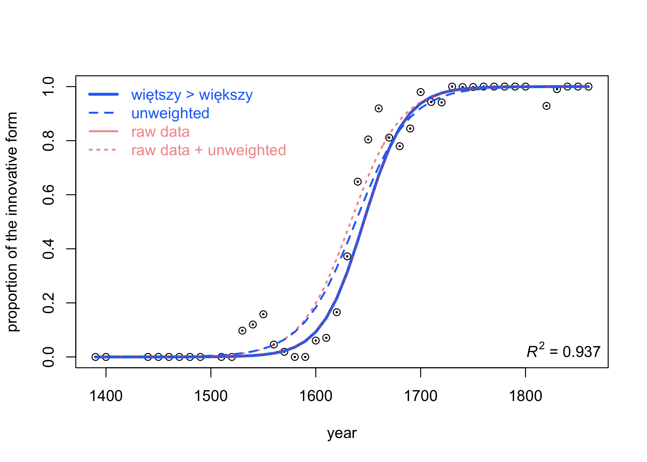
Figure 1: The change więtszy > większy. The points show the proportion between the recessive and innovative form (empirical data), the solid line presents a fitted logistic model with prior weights, whereas the dashed line – an unweighted model (i.e. simple logistic regression). Two other lines show models inferred from a raw dataset, discretized at the level of one year.

The plot shows four logistic regression models, denoted with solid, dashed and dotted lines. They appear to be similar yet it is not obvious at all which of them optimally describes the original dataset. Before we can claim any of the models valid, their statistical significance needs to be assessed. To this end, we will be using standard diagnostic tools: the p-value as a measure of statistical significance, and R² for assessing the goodness-of-fit. Since the original R² measure is shown to be misleading in logistic regression setups, we use a pseudo-R² variant as proposed by McFadden (1973). Whenever we report any R² values hereafter, we mean McFadden’s pseudo-R² measure.

In case of the change więtszy > większy, the data points follow the idealized curve very closely, as if the curve was attracting them – arguably, the logistic regression describes the observed data very well. This intuition is corroborated by a very high statistical significance, $p<0.001$, under the optimal parameters of the model ($\beta_{0}=-82.238$, $\beta_{1}=0.049$, at 42 degrees of freedom). The model is presented in Fig. 1 with a solid line. The goodness-of-fit, or the match of the logistic curve with the observed data, is also very high, with R² = 0.937.

The difference between the weighted model (solid line) and an unweighted one (dashed line) line is very small, yet noticeable. With the inferred parameters $\beta_{0}=-64.569$, $\beta_{1}=0.394$, the unweighted model exhibits the goodness-of-fit only marginally worse compared to the weighted version (R² = 0.932 vs. 0.937). The potential bias introduced by imbalanced input data does not appear to be significant, at least in this case (some advantages of using weighted models will be discussed later, see Fig. 4–5).

Certainly, a question might be asked whether a different size of the subcorpora and/or a different overlap of the moving window could have affected the results. Similarly, one might ask whether a model inferred from raw data – presumably as fine-grained as possible – would exhibit a different picture. While the former question will be discussed in the Evaluation section, here we briefly address the latter one. The dashed line in Fig. 1 represents a logistic regression model fitted to the raw dataset. Not only is the model statistically significant ($p<0.001$ at 200 degrees of freedom), but it is virtually indistinguishable from our base model involving bins (while the unweighted version follows a slightly different path, see Fig. 1, dotted line). It is true that the R² = 0.669 is much lower than in the base model, but this is due to the fitting conditions: a big number of degrees of freedom by definition produces more residuals and inevitably deteriorates R². For this reason, the value 0.0.669 cannot be directly compared to all the other R² scores discussed in the paper. Even though, the obtained goodness-of-fit for such a raw model can be claimed high.

6.2 barzo > bardzo

The second change is barzo > bardzo. Unlike other cases under our scrutiny, this is a relatively late change – it is virtually impossible to spot any attestations of the newer form until the early 17^th century. In our corpus, we noted only 25 occurrences of bardzo (not only in positive degree, but also in comparative as well as in superlative) with over 2,213 occurrences of the form barzo (and barziej and najbarziej) before the year 1600. From that moment on, the process of transition slowly accelerates; the rapid increase in the share of the innovative bardzo occurs at the end of the 18^th century. As shown in Fig. 2, the process is well described by logistic regression, with a high goodness-of-fit R² = 0.815, and even a higher value of 0.919 for the unweighted (i.e. simple) logistic regression model.

However, a deviation from the model in the second half of the 18^th century cannot be neglected. Two outliers that clearly differ from the modeled course of the change perhaps could be attributed to our data collection procedure: we have computed the frequencies collectively for the positive, comparative and superlative degree, while it could have happened that positive (barzo > bardzo) and comparative as well as superlative changed at a different pace. Also, it is possible that a single author – particularly conservative in this case – was responsible for this effect.

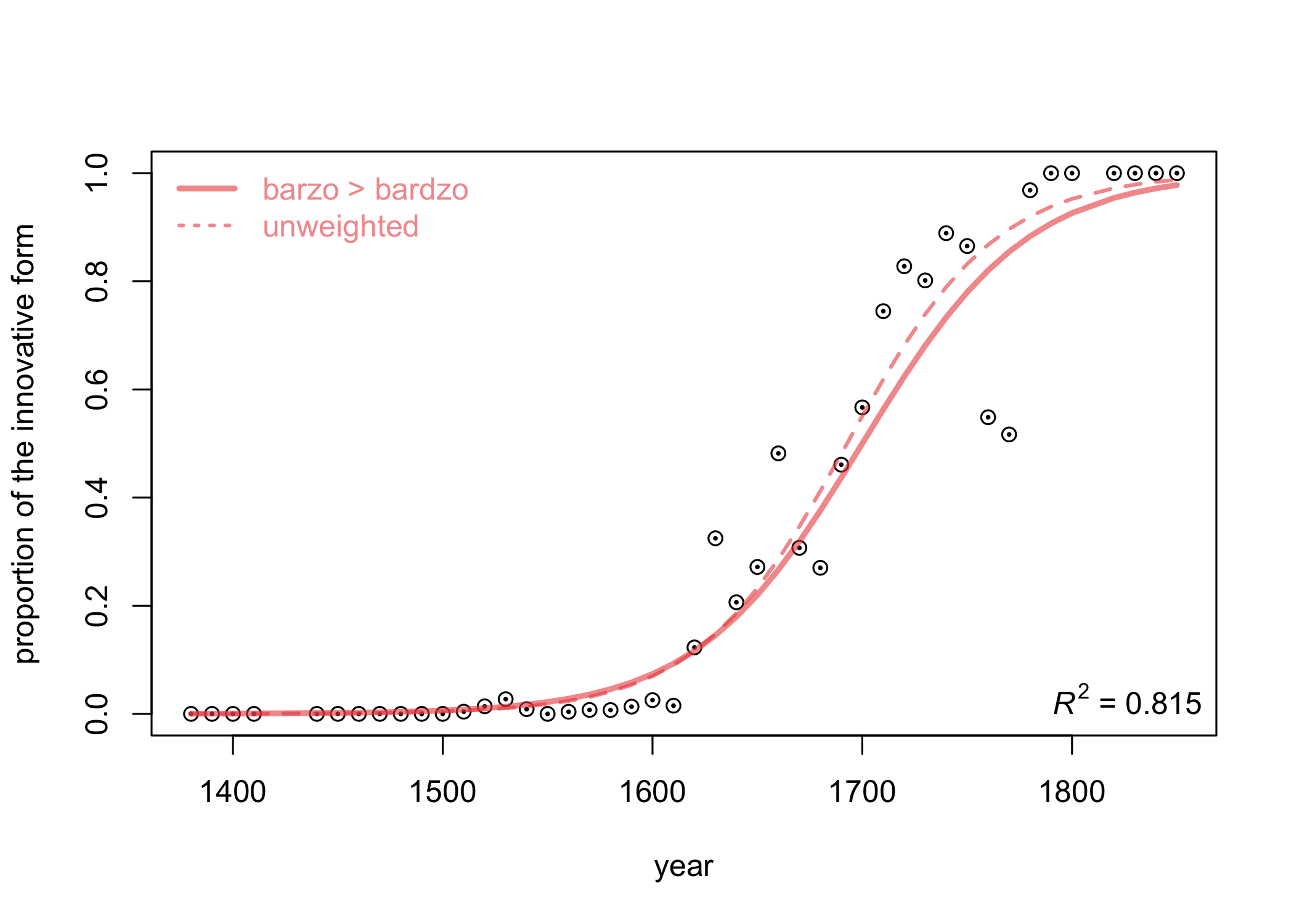
Figure 2: The change barzo > bardzo.

6.3 -bych > -bym, -bychmy > -byśmy

The late 15^th and early 16^th century witnessed the coexistence of -bym, -byśmy (the forms used in the present day Polish) and -bych, -bychmy as markers of the 1^st person singular and plural, accordingly. The competition of these two forms was studied, among others, by Taszycki (1946), Kowalska (1978), as well as Motyl (2014). Taszycki links the forms -bych, -bychmy with the region of Lesser (southern) Poland, since authors from elsewhere used it rarely. It was also noticed that the course of the change of the two morphemes was different – it persisted longer in the plural than in the singular.

Fig. 3 shows the course of change of the markers of both numbers together. The first thing that immediately catches the eye is the very good fit of the model to the data: -bych > -bym, -bychmy > -byśmy is a perfect example of logistic regression. The value of R² = 0.0.957 (or 0.976 for the unweighted model) at $p\approx 0$ only confirms the observations made by eyeballing.

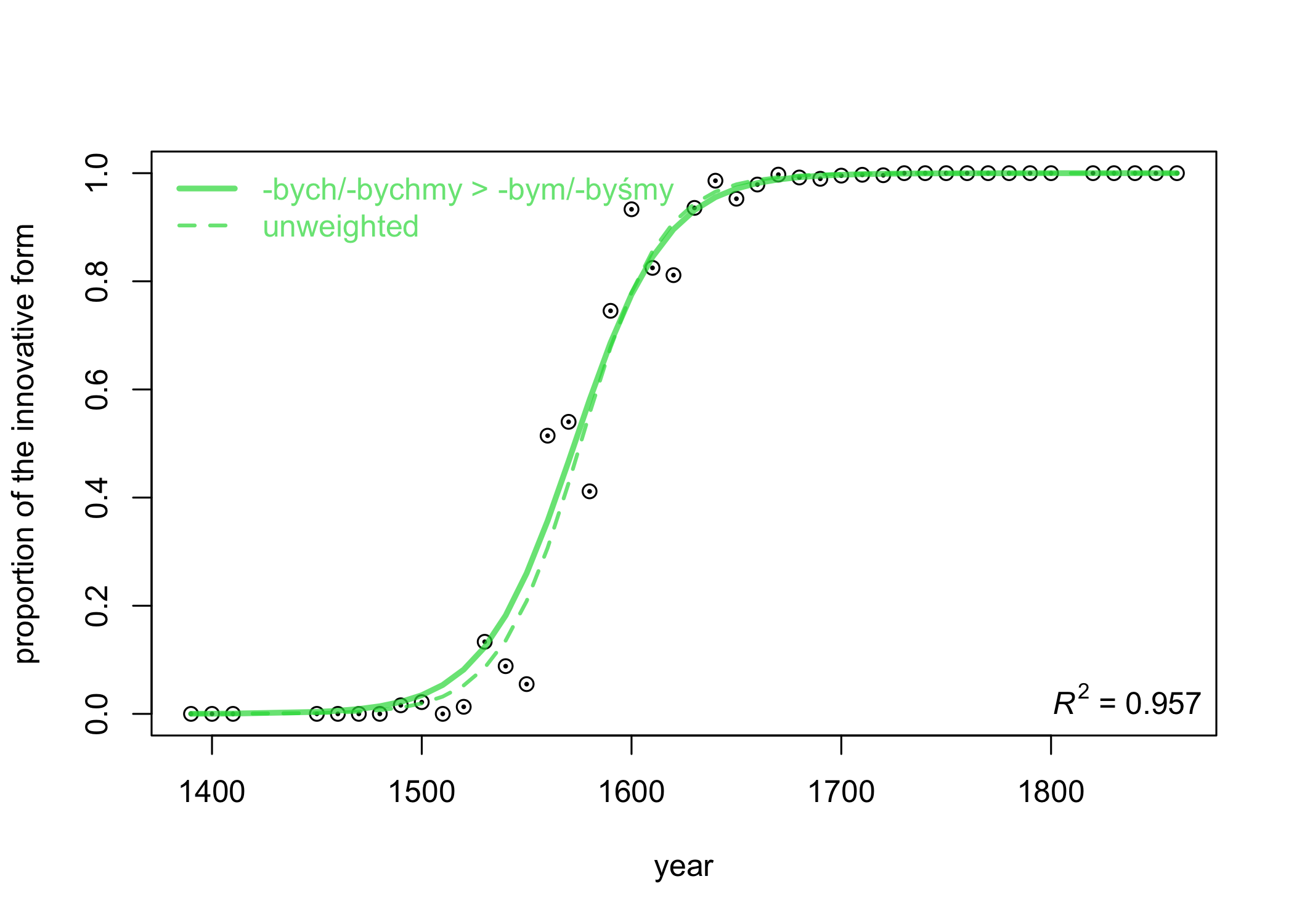
Figure 3: The course of change of -bych/-byśmy > -bym/-byśmy.

Two forms of the same verb – namely 1^st person singular and 1^st person plural – can be modeled together, as shown in Fig. 3, but they can be also scrutinized individually. Fairly plausible is a scenario in which one of the forms gains its popularity sooner, whereas the other form is following up at a slower pace. Therefore, we also computed independent models for the two forms (i.e. singular and plural). While the model for bych > bym alone proved to be virtually indistinguishable from the above combined approach, the plural form was different: the beginning of the change turned out to be blurry and therefore difficult to fit a logistic regression model. However, here we face a situation where making a model aware of data imbalance – by adding weights to the equation – improves the performance significantly. The weighted model not only exhibits a higher goodness-of-fit R² = 0.618 (vs. 0.558 for the unweighted variant), but it also resembles the “s”-curve to a greater extent (Fig. 4, solid vs. dashed line). The weighting effect can be appreciated with a naked eye: in Fig. 4, we log-scaled the data points according to the number of attestations in particular bins. While in the period 1450–1460 we deal with 7 occurrences of both forms, in the time span 1600–1610 the number of attestations reaches 451. Apparently, the weighted model pays less attention to the faint data points (including the outliers!) than to the opulent ones. If we assume that the textual evidence from early documents is on average less reliable than later sources, weighted logistic regression models might indeed be preferred over the classical models, let alone the original Piotrowski’s equation.

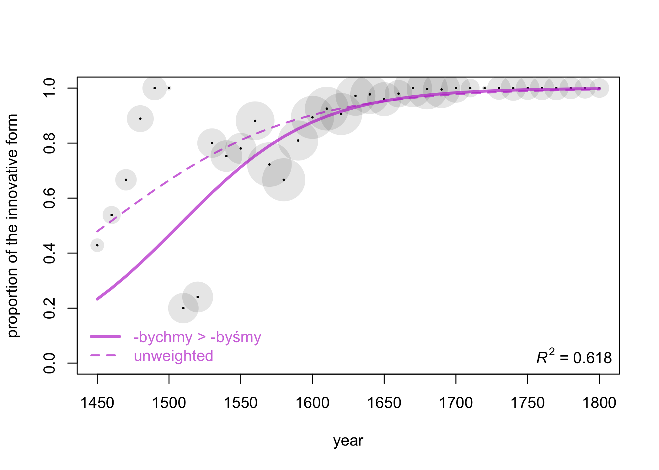
Figure 4: The course of change of the form bychmy > byśmy alone. The size of the data points is the natural logarithm of the number of attestations in each time span.

6.4 na- > naj-

Disregarding very few (and uncertain) occurrences of naj- in the 15^th-century part of our corpus, the first attestation of the innovative form can be dated 1535, while its recessive counterpart is noticed for the last time in 1772. As far as the 15^th-century period is concerned, the data points are highly blurred. Moreover, due to the overall scarcity of data in the 15^th century, the marginal occurrence of the innovative form in two psalters significantly increases the proportions of the innovative to the recessive form. The course of the change in the entire corpus is illustrated in Fig. 5.

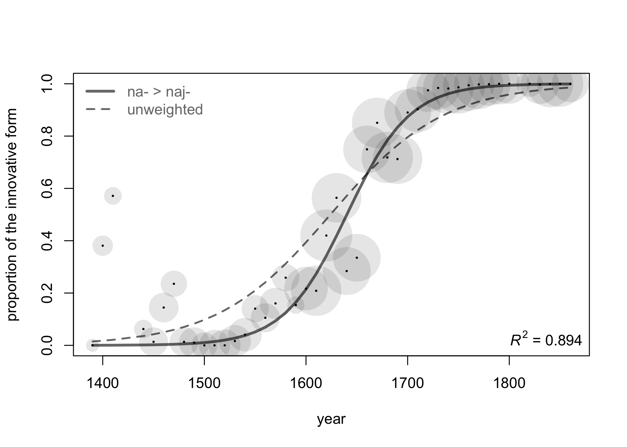
Figure 5: The course of change of the superlative marker na- > naj-. The size of the data points is the natural logarithm of the number of attestations in each time span.

Despite these blurred data points in the oldest Polish texts, the fit of the theoretical course of logistic regression to empirical data is not as bad as one might think, with R² = 0.818 at p < 0.001 (Fig. 5, dashed line). Here, the weighted variant of our model again proves superior, with its significantly higher R² = 0.894, and visually better trajectory (solid line). It appears, once more, that an imbalanced dataset can be corrected for with a weighted model.

6.5 -ir- > -er-

Fig. 6 depicts the competition of the forms with recessive -ir- and innovative -er-, such as e.g. śmirć > śmierć ‘death’, cirpieć > cierpieć ‘to suffer’, pirwej > pierwej ‘first, before’. As can be seen in the plot, this change is an imperfect example of the logistic process, since the corpus does not reveal the beginning of the change – the innovative form can be found already in the first subcorpus. The proportion of the innovative form raises consistently. Another untypical feature is a very long period when the recessive forms are barely attested. It seems that the process of this change was completed in the beginning of the 17^th century, but the archaic forms occasionally emerged in the course of the next two centuries. One possible explanation is that the speed of the change is different for particular words. It is also possible that in the 18^th century there was a kind of temporary return to the archaic form motivated by a fashion. Since the beginning of the change remains hidden in the pre-literate era and thus invisible to the logistic model, it comes as no surprise that the fit of the model, R² = 0.619 (and 0.853 in the unweighted variant), is lower than in the cases discussed above, yet still acceptable.

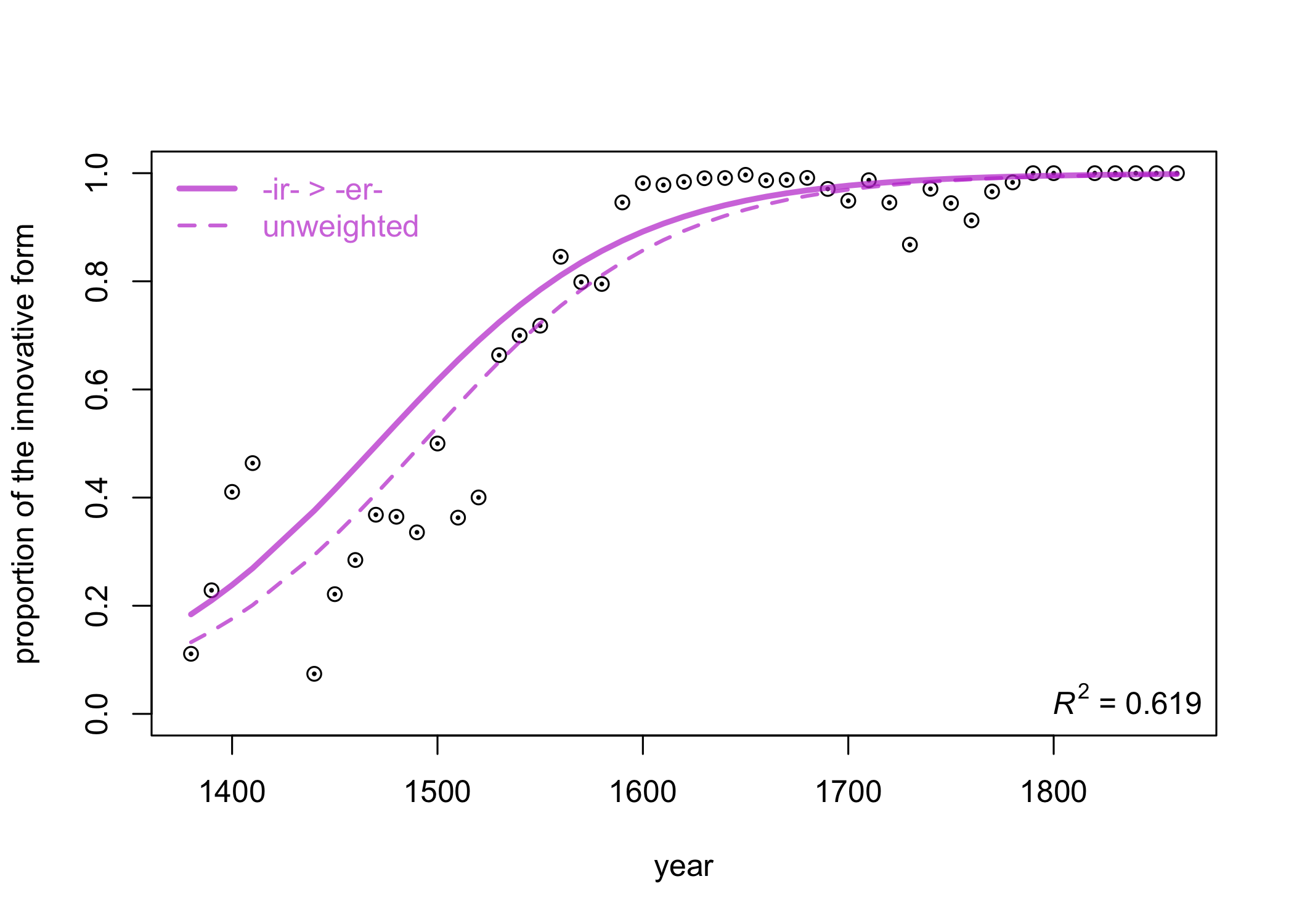
Figure 6: The course of change -ir- > -er-.

6.6 inszy > inny

This change can hardly be described in terms of logistic regression in its standard form. Should we restrict ourselves to the procedure which we applied so far, little could be said about the nature of the process. The goodness of fit of such a model is unsatisfactory, with R² = 0.488. The performance of a weighted model proves substantially better, with R² = 0.655 (Fig. 7, dotted line), yet one cannot deny the fact that the data points hardly follow a logistic trajectory. Two immediate conclusions can be formulated here: firstly, Piotrowski’s original idea of modeling the change by an “s”-shaped curve does not apply universally, and therefore it cannot be referred to as a linguistic law. Secondly, while standard logistic regression model proves unsatisfactory, other options from the generalized regression family can be used instead. And indeed, the polynomial logistic regression model (James et al., 2013: 265–300) seems to be a good choice here. The principle of such a model, in a nutshell, is that instead of limiting the modeled curve to the “s” shape, we allow for its greater flexibility. Depending on the degree of the polynomial, the line may bend many times; each subsequent parameter of the polynomial allows for two additional bends.

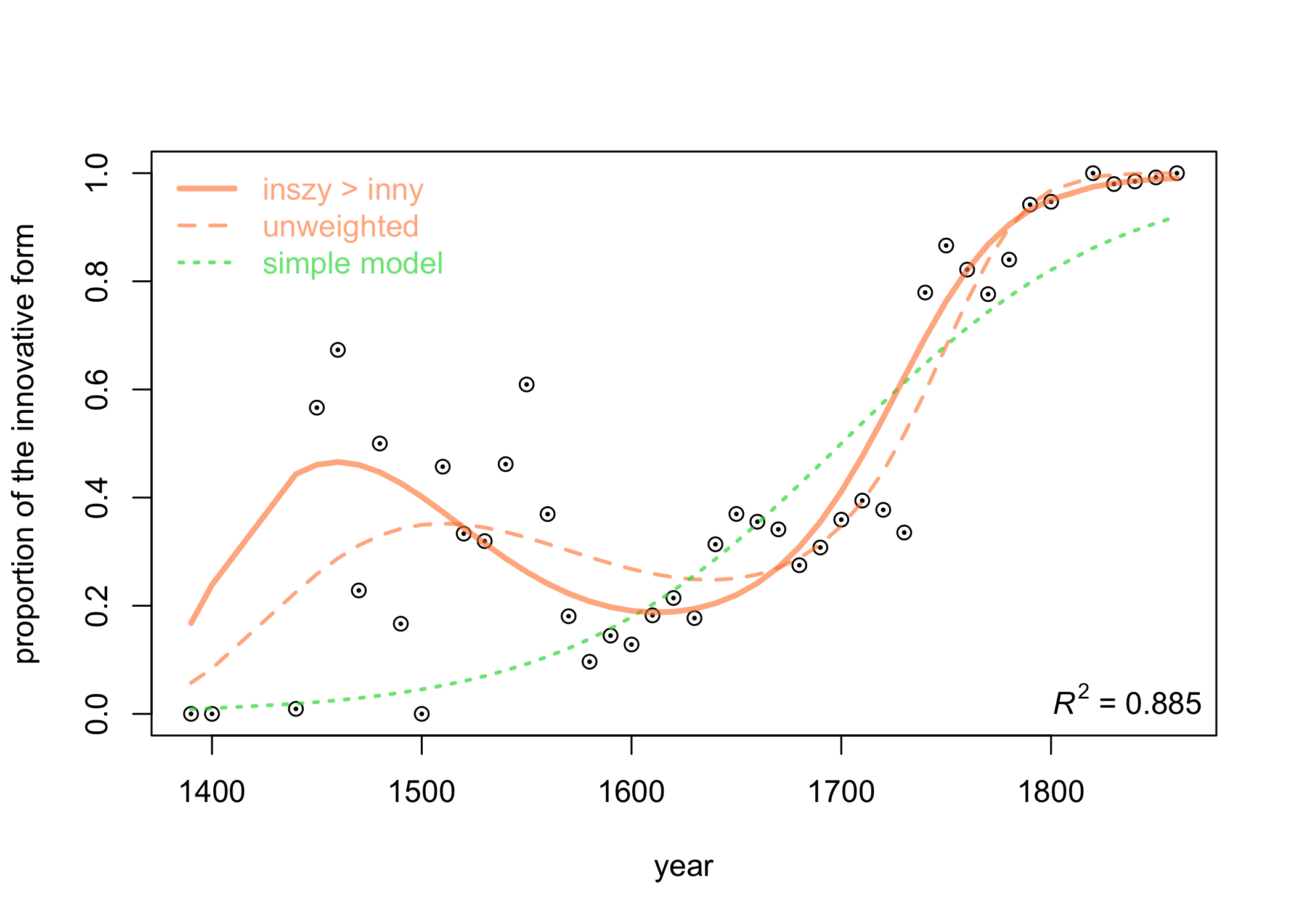
Figure 7: The course of change inszy > inny (in all inflected forms). Polynomial logistic regression model with prior weights (solid line) and unweighted (dashed line) vs. simple logistic regression (dotted line).

Fig. 7 shows a model that uses a 3^rd degree polynomial. As one can see, the model follows the empirical data sufficiently yet not optimally, which is confirmed by a relatively decent fit of the model, R² = 0.885 at p < 0.05 (and 0.655 for the unweighted model). Certainly, higher-order polynomials would lead to a better fit (and ultimately to overfitting), but at the same time all these complex models have to be rejected because of their high p-values. Still, even the 3^rd degree polynomial does not seem to explain the dispersion of data points in the years 1450–1550. Note, however, that after 1550 the course of the change follows the classical logistic curve: if we only took into account the data from this year and used the classical model, the value of R² would increase substantially.

6.7 wszytek > wszystek

The change wszytek > wszystek ‘all’ has already been discussed in literature (Michalska, 2013; Klemensiewicz, 1965), yet with no quantitative evidence taken into account. Interestingly, large-scale material excerpted from our diachronic corpus does not exhibit a clear picture either. To be precise, it is difficult to identify a clean Piotrowski’s process here (Fig. 8). Although the trend stabilizes in the second half of the 18^th century and is substantially closer to the expected “s”-shaped curve, for the most part the results are very blurred. Even the use of a polynomial logistic regression model does not help much: despite the decent degree of model fit, R² = 0.784 when using a 3^rd degree polynomial, it can be easily seen that for the period covering the 15^th–17^th centuries, the distribution of points does not resemble the modeled curve. Fitting to empirical data can be artificially increased by using a model with a higher degree of the polynomial (e.g. for a 4^th degree polynomial R² = 0.837), nonetheless, such a model doesn’t show statistical significance any more (the p-value increases well beyond the 0.05 level), which simply means that the model does not sufficiently describe the data.

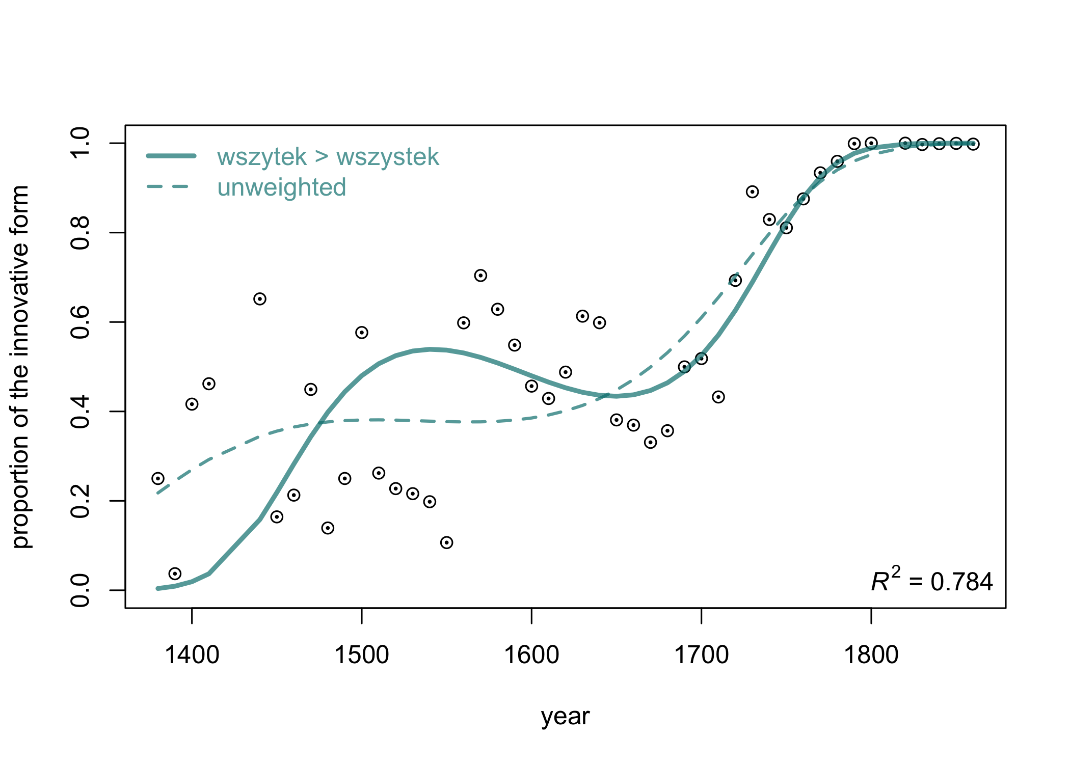
Figure 8: The course of change wszytek > wszystek (in all inflecting forms).

Again, an immediate observation can be made about the validity of Piotrowski’s “law”. This time, however, data scarcity cannot be blamed for the remarkable dispersion of the data points spanning over the 14^th–17^th centuries. The change wszytek > wszystek with its 55,005 attestations is our best documented case.

6.8 Competing forms abo and albo

In the case of abo and albo ‘or’ we don’t observe a transition from one form to another, but rather a competition of two forms. In the Middle Ages, albo was typical for southern Poland, whereas the northern regions adhered to abo (Michalska, 2013). Moreover, the latter form was considered to belong to lower registers – hence its absence in religious texts. In the 16^th century abo percolates to all regions and all genres. It has also been suggested that the spread of abo in high brow texts is due to a typo mistake in the 1560 edition of the very popular Postil by Mikołaj Rej (Urbańczyk, 1953). Whatever the actual reason of the change might be, important in the context of our study is the accelerating growth of abo at the cost of albo. In the first centuries the trajectory resembles Piotrowski’s process. Just a few decades before winning the game, however, the form abo unexpectedly derails: starting from the mid-17^th century, the almost-extinct form albo gradually regains its position of a ruler, eventually pushing abo into the status of archaism in the 19^th century.

Using a standard logistic model would not yield any acceptable results in this case, since the curve (see Fig. 9) does hardly resemble the shape of an “s”. Instead, the polynomial logistic regression model seems to better describe such a non-obvious competition of two forms. The goodness-of-fit is relatively high, R² = 0.868 when a 6^th degree polynomial is used (R² = 0.803 for the unweighted model). Although the model is rather complex, with multiple parameters, and difficult to defend against Occam’s razor, it nevertheless explains the empirical data decently.

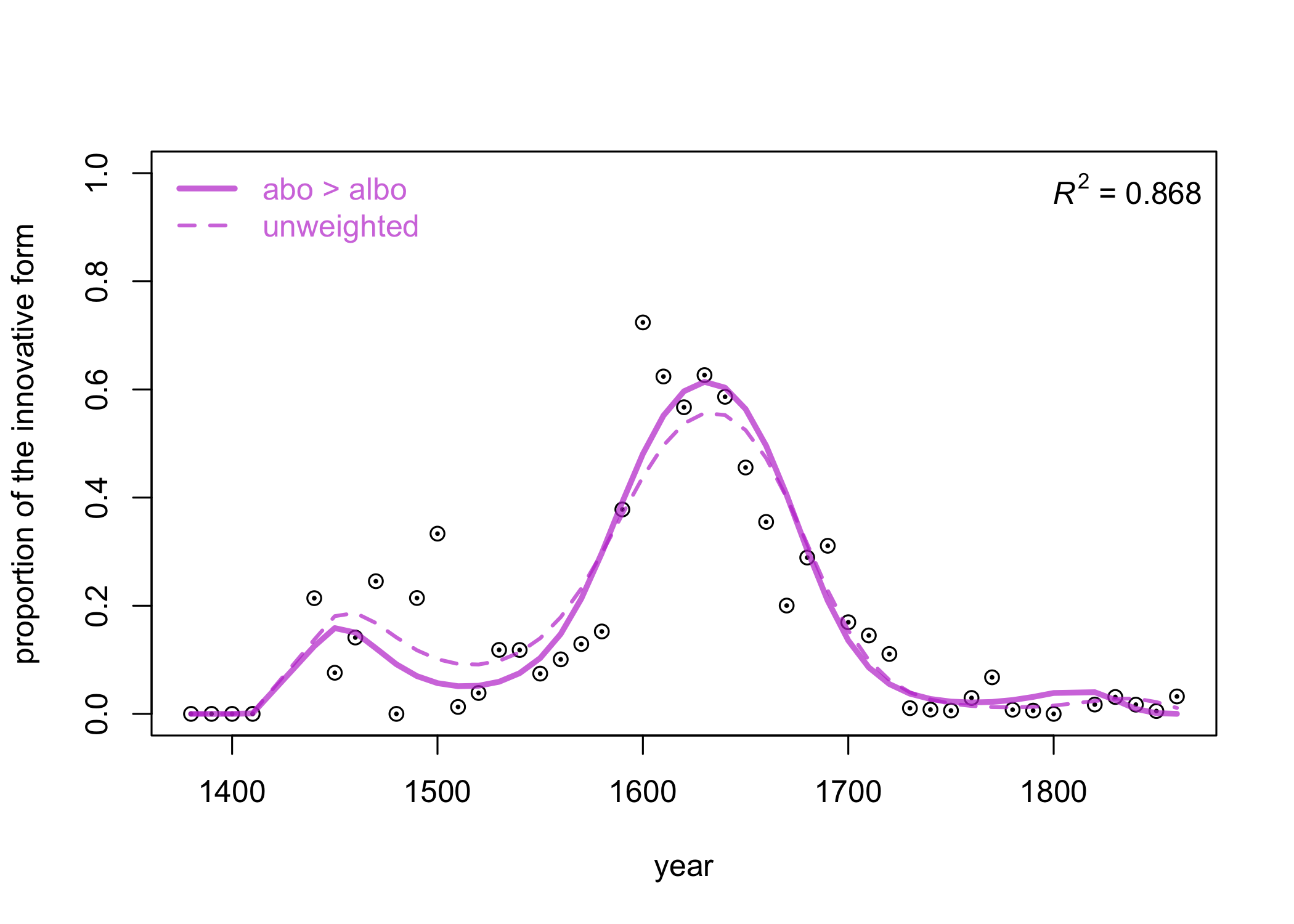
Figure 9: The competing forms abo and albo: a model of polynomial logistic regression.

From a theoretical point of view, the competition of abo and albo can also be viewed as a combination of two logistic curves, one of which would mirror the other: ideally, a raising curve (which can be imagined as the lower part of the letter “s”) would smoothly evolve into its mirror image, or a descending curve, as was proposed by Vulanović (2007: 113). Fig. 10 shows exactly the same dataset for abo and albo, but this time it has been split into two parts and modeled independently of each other, using classical logistic regression. As it turns out, the first part (1380–1610) fits to the model to a much lesser extent (R² = 0.47) than the second part (R² = 0.921). Also, the hypothesis of two mirror logistic curves finds no confirmation in our data: in different scenarios that we tested, the two best-fit models never matched, no matter where the split into the two parts was applied.

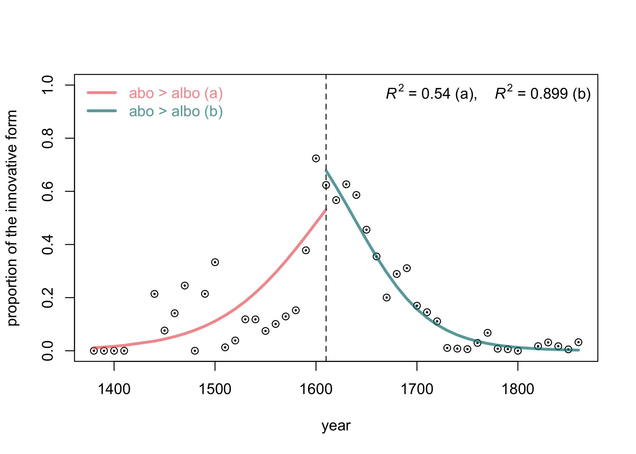
Figure 10: The competing forms abo and albo: two independent logistic models computed separately for two time spans, 1380–1610 and 1610–1850.

The results shown in Figs. 9 and 10 might give an impression that they describe two substantially different courses of change abo > albo. However, this is only an illusion, as the data points (black dots) in both plots are identical. Different varieties of lines, colors or shapes superimposed on a graph strongly affect our perception of actual data – the effect is known as visual rhetoric bias. This leads us to a two-fold observation. Firstly, the models discussed above reconstruct different trajectories of change – in our situation it is either a two-hump run (Fig. 9) or a one-hump run (Fig. 10) – and it is not obvious at all which of the two models is more likely to tell the truth. Secondly, the eyeballing is prone to bias – as we have seen above – hence the need to supplement the plots with the goodness-of-fit measures, such as R² or one of its variants.

6.9 The dynamics of language change

Given the above results discussed individually, a natural question emerges of how the particular changes relate one to another. Do they travel through time in a collinear fashion? Although we have no reason to suspect a perfect overlap of the changes nor a particular order (the changes are not caused one by another), yet still, the question remains as to the general dynamics of language change. Do all the changes advance at the same pace? It has already been suggested that a few individual logistic curves might be combined into a single multidimensional model (Vulanović, 2012). However, in our study we propose a somewhat simpler approach, namely we suggest to focus first on a composite picture of all the trajectories merged into one plot (Fig. 11), which shows a gradual accumulation of several individual (independent) changes.

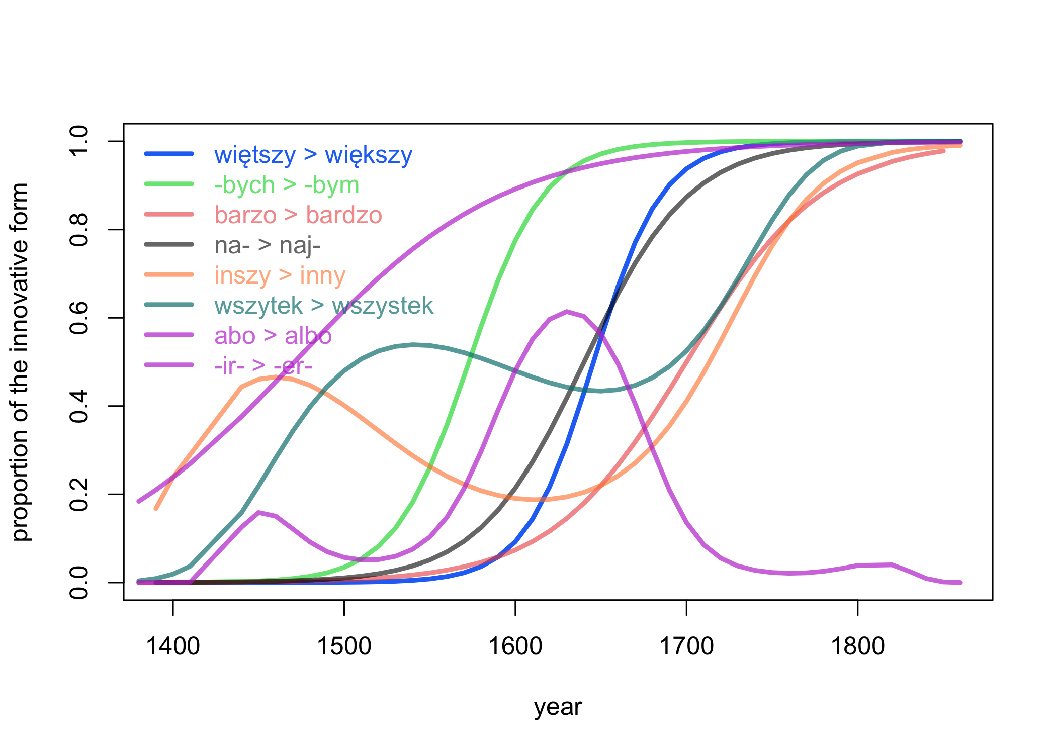
Figure 11: The overall picture of the language changes in Middle Polish.

The complex symphony of individual models represented in one plot shows how different the dynamics of the diachronic process can be. While na- > naj- is a slow, time-stretched process, then -bych > -bym is a sudden change, so is also więtszy > większy. What makes these processes different, is the fact that they happen at a different time – when the probability of the innovative -bym is already close to 1, the probability to find the innovative form większy is barely reaching 0.5. To put it simply: when the former process is about halfway through, the latter is at its beginning. If, on the other hand, we compare -bych > -bym to barzo > bardzo, we find that the second process is even more recent (it starts when -bych already disappears from the system) and meanwhile somewhat slower, which can be seen from the more gentle slope of the modeled line.

Since one could expect the changes to occur at different times, the lack of any collinearities or consistent breakthroughs in, say, 16^th or 17^th century, is rather surprising. If such a collinearity had surfaced, if would have supported the hypothesis that a language change is a combination of several variables occurring roughly at the same time. Our results suggest otherwise that it is difficult to identify a clear-cut moment of a general language change; rather, we deal here with a gradual accumulation of several individual (independent) changes.

7 Evaluation

No matter how convincing the presented results might seem, a crucial question has to be asked: to which extent are these results stable and reproducible? In the following section, we will address the issue by a systematic examination of the conditions of our experimental setup.

There are at least three elements of the procedure that might have affected the final model. Firstly, since the shape of the logistic curve is a derivative of the estimated parameters $\beta_{0}$ and $\beta_{1}$, one could ask whether any distortions might appear at this stage of modeling. Arguably, there is no room for manipulation here: the parameters $\beta_{0}$ and $\beta_{1}$ are estimated by solving an equation that minimizes the difference between the model and empirical data (James et al., 2013: 133–34). There exists only one pair of values that satisfies the equation, therefore it is not possible for the result to be tweaked at this stage. A given set of input values will always give one optimal solution, even if the curve does not look optimal to the human eye.

The second source of distortions is, obviously, the input dataset itself: it is rather naïve to expect that solid results could be obtained from a corpus of poor quality. Although this component has an immense impact on the entire experiment, there was little we could do about it, apart from collecting as many texts as possible and checking the individual texts for quality. Still, we assume that the amount of systematic error we potentially deal with, is an inherent feature of the dataset and does not change from one experiment to another.

Finally, the third source of possible distortions is our procedure of dividing the data into smaller subcorpora, as discussed above in the Method section. Analyzing diachronic phenomena always requires the dataset to be divided into smaller time spans, therefore no objections can be raised as to the idea of splitting. What calls for explanation, however, is the size of a single time span. As mentioned above, the chosen subcorpus size should account for data scarcity, while keeping the noise at the lowest possible level.

While the choice of the subcorpus size might be – and usually is – somewhat arbitrary, the size of the overlap between particular subcorpora is even more so. Again, we can assume that a large overlap size (i.e. a slow pace of the moving window) results in smoother data points, but it comes at the cost of their reliability, especially when a single outlier falls into several subcorpora at a time. Due to the lack of strong theoretical assumptions, both the subcorpus size and the overlap have to be decided by choosing the combination of parameters that yield best results.

We approached the above issue empirically, by testing numerous possible combinations of the subcorpus size and the overlap in a grid-search manner. We conducted a series of tests for 20 different sizes of the subcorpora: 5, 10, 15, 20, …, 100 years, and for 20 different sizes of the overlap, modeling the 7 linguistic changes discussed above (we excluded abo > albo, and merged -bych > -bym and -bychmy > -byśmy into one instance) for a total of 2,400 models for comparison. In fact, we were able to compute the parameters for only 1,200 models, since the overlap size cannot exceed the current subcorpus size. For each of the models, we calculated the R² coefficient of goodness-of-fit. We repeated the entire procedure for both weighted and classical logistic regression models. Due to the fact that the general picture turned out to be similar in these two groups of models, below we report the R² values for the unweighted variant only. A small portion of results for the 50-year subcorpora with an overlap of 20 years, and the 20-year subcorpus with an overlap of 5 years, are presented in Table 1.

change	subcorpus 50 years	subcorpus 20 years
więtszy > większy	0.952	0.921
-bych > -bym	0.983	0.954
barzo > bardzo	0.903	0.818
na- > naj-	0.950	0.898
inszy > inny	0.937	0.887
wszytek > wszystek	0.856	0.779
-ir- > -er-	0.647	0.608

Table 1. Goodness-of-fit of the logistic model to empirical data (McFadden’s pseudo-R²) depending on different ways of dividing data into subcorpora.

With the large number of results for 1,200 independent test, discussing them individually would be difficult, therefore we present them in a compact form in Figs. 12–13. The plots show the goodness-of-fit as a function of the subcorpus size, for a 10-year overlap and for a 20-year overlap, respectively. Relatively high R² for big subcorpora (say, of 50 or 100 years) comes at no surprise given the smaller number of degrees of freedom and the smoothing effect of large moving windows, but the actual goal here is to decrease the subcorpus size as far as possible while still observing acceptable results. The general picture is fairly optimistic, since we don’t encounter any substantial decrease of R² for subcorpora between 20 and 100 years. Below the value of 20 years, the performance of modeling decreases significantly.

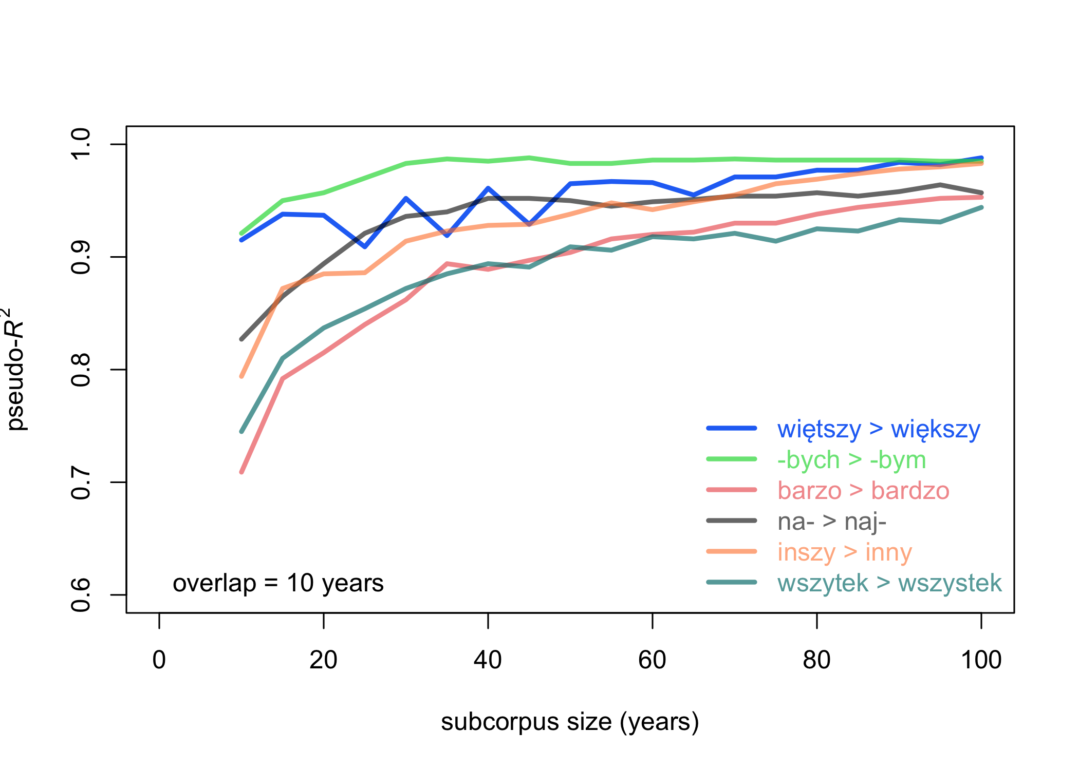
Figure 12: The influence of the subcorpus size on the goodness of fit (10-year overlap).

When it comes to the overlap size, the differences between Fig. 12 and Fig. 13 clearly show that a small overlap – which can be also interpreted as a fast pace of the moving window – produces smoother results than slowly moving windows. Arguably, we are observing here an effect of the outliers falling into several subcorpora when the window progresses too slowly.

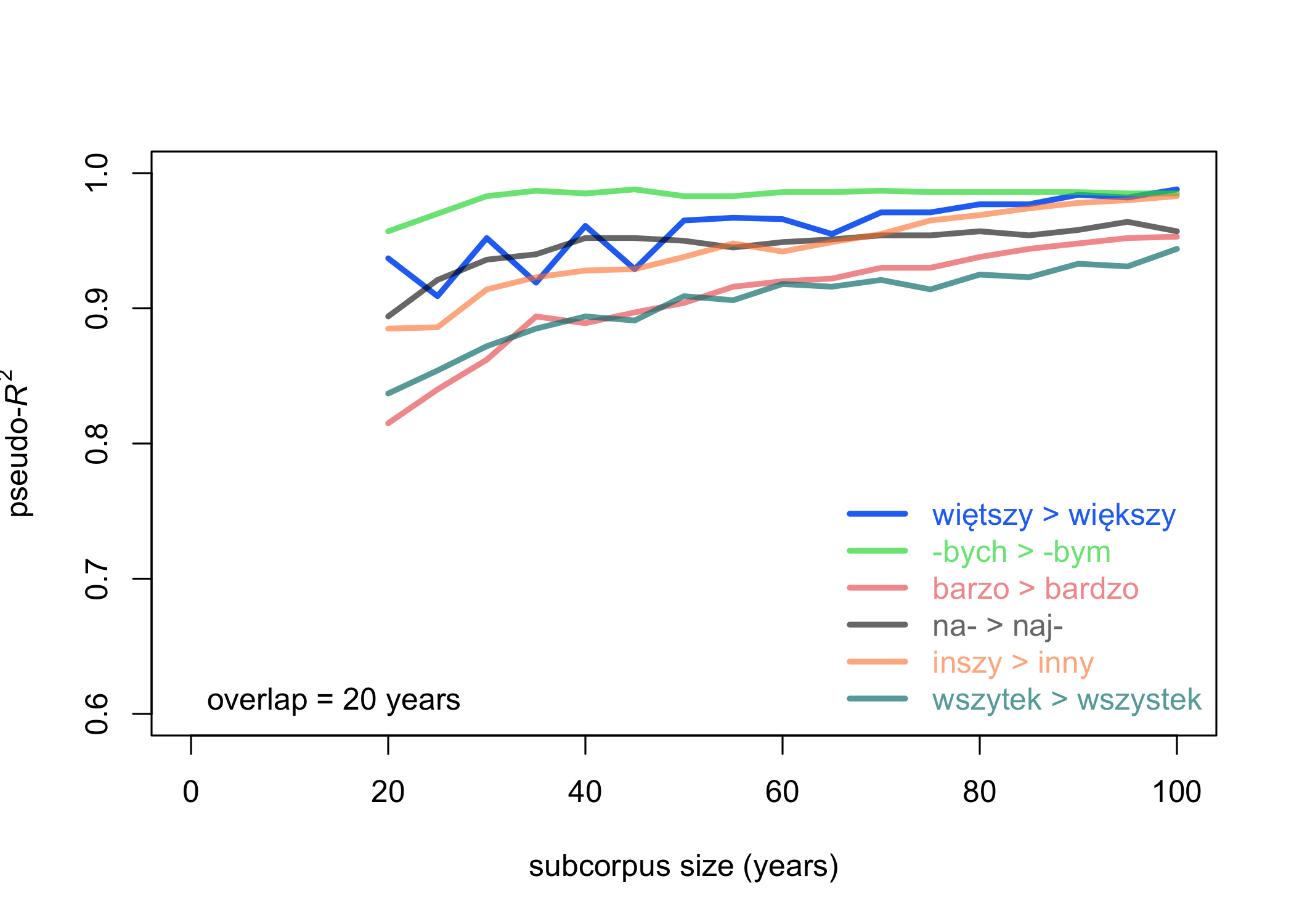
Figure 13: The influence of the subcorpus size on the goodness of fit (20-year overlap).

The evaluation tests allow us to draw a few conclusions. Firstly, the relatively stable R² across the board might suggest that the underlying logistic processes for our discussed changes are perhaps stronger than we suspect; apparently, dividing the corpus arbitrarily into any subcorpora of 20 or more years would still yield satisfactory results. Secondly, thanks to the above systematic tests we have gain empirical justification for the arbitrary size of the subcorpus discussed in the previous sections, namely 20 years with a 10-year overlap.

8 Discussion

The results presented in this study exhibit a reasonable predictive power, namely the goodness-of-fit for particular logistic regression models turned out to be rather high. The best fit reached R² = 0.957, and rarely dropped below 0.7. There is a fly in the ointment, though. No matter how many cases follow the expected course of change, the exceptions from the model cannot be denied. Sooner or later, one arrives at a case when the observed results do not resemble any “s”-shaped trajectory and yet, insufficient amount of data cannot be blamed for the effect. It is true that sometimes a more complex variants of the logistic models can yield reasonable results. However, this hardly satisfies a historical linguist, who might want to ask: Why do some changes follow the model, while others don’t? Or perhaps a valid question is the opposite one: why should we expect the changes to always follow the logistic curve? Language can be affected by several – internal and external – factors; a conservative school education system can slow down the changes, and the same goes for the prescriptive linguistics’ authority, whereas progressive literary influencers or, in more recent times, social media can accelerate the changes substantially. Why wouldn’t other variables play role in this fairly complex picture?

The reservations formulated above shed some light on the nature of language changes examined in this study. We refer to them as the so-called Piotrowski’s law, because we hardly believe one deals here with any linguistic quantitative law in the sense of Zipf’s, Menzerath’s or Heaps’s law. For in the classical sense, a quantitative linguistic law in order to be named as such must occur under all conditions and in every language – it must be universal. In contrast, the process observed by Piotrowski applies only to a certain group of linguistic changes. Therefore, we rather agree with Stachowski that such a non-linear process does not actually apply to language and its self-organization (as many other laws of quantitative linguistics do), but to social processes related to language (Stachowski, 2020).

9 Conclusion

In this paper, we examined a few changes in Polish over the relatively wide time span of 15^th–19^th centuries, some of them being successful realizations of the so-called Piotrowski’s law. In order to quantify these cases, we used logistic regression modeling, followed by the p-value and the R² coefficient to assess the model’s goodness-of-fit. We also extended the standard approach by using general logistic regression models with polynomial kernels, for the cases which hardly resemble Piotrowski’s process. Yet, even the polynomial models could not explain the changes that exhibited a considerable dispersion of data points. This oftentimes applied to early periods of Polish, whereas the evidence for 17^th–19^th centuries usually showed a better match with the models.

The set of changes which we have chosen for our study are documented in a single corpus, and they run concurrently. This offers a unique opportunity not only for comparing the fit of the models to each dataset individually, but also to observe how they relate one to another. Our results clearly show that the changes that have been traditionally (yet tacitly) assumed to exhibit similar dynamics, are in fact very different in their trajectories.

The observation that needs to be commented on, is that some of the changes are not compliant with the model or, to be precise, with the standard logistic regression model of phase change. Since the change abo > albo can be explained by a failed innovation scenario, the other irregular changes don’t fall into this category at all. Moreover, in some cases the blurry picture cannot be simply explained by data scarcity. Presumably, our results show once more that the logistic “s”-shaped trajectory, though it describes most of the processes to an acceptable degree, cannot be considered a universal underlying rule for the language change. While some exceptions from the so-called Piotrowski’s law have been already reported in the literature, our study provides new and rich evidence of this phenomenon.

Last but not least, our experiment shows that even a relatively small diachronic corpus (12 million words in total) is large enough to trace language changes over the course of a few centuries. This is a fairly optimistic outcome, because diachronic corpora will always suffer from insufficient coverage and the lack of balance. We would like to hope that our findings can serve as an encouraging example for further investigations.

10 Acknowledgements

This research was conducted as a result of a project supported by Poland’s National Science Centre (project number UMO-2013/11/B/HS2/02795).

References

Altmann, G. (1983). Das Piotrowski-Gesetz und seine Verallgemeinerungen. In Best, K.-H. and Kohlhase, J. (eds), Exakte Sprachwandelforschung. Theoretische Beiträge, Statistische Analysen Und Arbeitsberichte. Göttingen: Edition Herodot, pp. 54–90.

Basu, A. (2016). ‘Ill shapen sounds, and false orthography’: A computational approach to Early English orthographic variation. In Ullyot, M., Jakacki, D. and Estill, L. (eds), Early Modern Studies and the Digital Turn. (New Technologies in Medieval and Renaissance Studies 6). Toronto & Tempe: Iter & ACMRS, pp. 169–201.

Best, K.-H. (1983). Zum morphologischen Wandel einiger deutscher Verben. In Best, K.-H. and Kohlhase, J. (eds), Exakte Sprachwandelforschung. Theoretische Beiträge, Statistische Analysen Und Arbeitsberichte. Göttingen: Edition Herodot, pp. 107–18.

Best, K.-H. (2013). Iranismen im deutschen. Glottometrics, 26: 1–8.

Gnatchuk, H. (2015). Anglicisms in the Austrian newspaper ‘Kleine Zeitung’. Glottometrics, 31: 38–49.

Górski, R. L., Król, M. and Eder, M. (2019). Zmiana w języku. Studia kwantytatywno-korpusowe. Kraków: IJP PAN.

James, G., Witten, D., Hastie, T. and Tibshirani, R. (2013). An Introduction to Statistical Learning with Applications in R. New York: Springer.

Klemensiewicz, Z. (1965). Historia języka polskiego. Warszawa: PWN.

Kowalska, A. (1978). Rozwój nowych form słowa posiłkowego: jestem, jesteś, jesteśmy, jesteście. Poradnik Językowy, 9: 377–84.

Köhler, R. and Tuzzi, A. (2015). Linguistic modelling of sequential phenomena. In Mikros, G. K. and Macutek, J. (eds), Sequences in Language and Text. Walter de Gruyter, pp. 109–23.

Leopold, E. (2005). Das Piotrowski-Gesetz. In Köhler, R., Altmann, G. and Piotrowski, R. (eds), Quantitative Linguistik – Quantitative Linguistics. Ein Internationales Handbuch. Berlin / New York: de Gruyter, pp. 627–33.

McFadden, D. (1973). Conditional logit analysis of qualitative choice behavior. In Zarembka, P. (ed), Frontiers in Econometrics. New York: Academic Press, pp. 105–42.

Meyer, C. F. (2002). English Corpus Linguistics: An Introduction. Cambridge: Cambridge University Press.

Michalska, P. (2013). Status staropolskich oboczności wyrazowych w polszczyźnie doby średniopolskiej. Poznań: Wydawnictwo PTPN.

Motyl, A. (2014). Normalizacja fleksji werbalnej w zakresie kategorii czasu w dobie średniopolskiej. Poznań: Wydawnictwo PTPN.

Piotrowskaja, A. and Piotrowski, R. (1974). Matematičeskie modeli v diachronii i tekstoobrazovanii. In Piotrowski, R. (ed), Statistika reči i avtomatičeskij analiz teksta. Leningrad: Nauka, pp. 361–400.

Stachowski, K. (2016). German loanwords in Polish and remarks on the Piotrowski-Altmann law. Issues in Quantitative Linguistics 4. Lüdenscheid: RAM-Verlag, pp. 237–59.

Stachowski, K. (2020). Piotrowski-Altmann law: State of the art. Glottotheory, 11(1): 3–14.

Taszycki, W. (1946). Staropolskie formy czasu przeszłego ‘robiłech’, ‘robilichmy’. Sprawozdania Polskiej Akademii Umiejętności, vol. 46. pp. 7–10.

Urbańczyk, S. (1953). Rola wielkich pisarzy odrodzenia na tle innych czynników kształtujących język literacki. Warszawa: Polska Akademia Nauk.

Vulanović, R. (2007). Fitting periphrastic “do” in affirmative declaratives. Journal of Quantitative Linguistics, 14(2-3): 111–26.

Vulanović, R. (2012). A multidimensional generalization of the Piotrowski-Altmann law. Methods and Applications of Quantitative Linguistics: Selected Papers of the 8th International Conference on Quantitative Linguistics (QUALICO). Belgrade, pp. 184–93.

Vulanović, R. and Baayen, H. (2007). Fitting the development of periphrastic “do” in all sentence types. In Grzybek, P. and Köhler, R. (eds), Exact Methods in the Study of Language and Text: Dedicated to Gabriel Altmann on the Occasion of His 75th Birthday. Berlin: de Gruyter, pp. 679–88.