Integrable modulation, curl forces and parametric Kapitza equation with trapping and escaping

Abstract

In this present communication the integrable modulation problem has been applied to study parametric extension of the Kapitza rotating shaft problem, which is a protypical example of curl force as formulated by Berry and Shukla in [J. Phys. A $\mathbf{45}$ 305201 (2012)] associated with simple saddle potential. The integrable modulation problems yield parametric time dependent integrable systems. The Hamiltonian and first integrals of the linear and nonlinear parametric Kapitza equation (PKE) associated with simple and monkey saddle potentials have been given. The construction has been illustrated by choosing $\omega(t)=a+b\cos t$ and that maps to Mathieu type equations, which yield Mathieu extension of PKE. We study the dynamics of these equations. The most interesting finding is the mixed mode of particle trapping and escaping via the heteroclinic orbits depicted with the parametric Mathieu-Kapitza equation which are absent in the case of non parametric cases.

PACS numbers

: 45.20.-d, 05.45. -a, 45.50.Jf

2000 Mathematics Subject Classification

34A05, 01A75, 70F05, 22E70.

Keywords and Key phrases:

First integrals; Curl force; Eisenhart-Duval lift; Kapitza equation; Higher-order saddle potentials; Mathieu equation; Heteroclinic orbits; Particle trapping and escaping;

1 Introduction

Berry and Shukla [1, 2] introduced Newtonian dynamics driven by forces $F({\bf r})$ depending only on position ${\bf r}$ and not on velocity ${\bf v}$ such that whose curl is not zero, hence they are not derivable from a scalar potential. The curl flow preserves volume in the position-velocity phase space $({\bf r},{\bf v})$ where there are no attractors. Given a curl force (assuming unit mass for convenience) $\ddot{\bf r}=F({\bf r})$, $\nabla\times F({\bf r})\neq 0$, we obtain

$$\nabla_{\bf r}{\bf v}+\nabla_{\bf v}\dot{\bf v}=\nabla_{\bf r}{\bf v}+\nabla_{\bf v}F({\bf r})=0,\qquad{\bf v}=\dot{\bf r}.$$

In early 90s Moser and Veselov [3] considered the family of integrable Hamiltonians $H(p,x;\Omega)$ depending on parameters $\Omega=(\omega_{1},\omega_{2},\cdots\omega_{n})$, which they made the parameters time dependent $\Omega=\Omega(t)$ with the time period $T$. In general this destroys the integrability structure of the system, they considered a special case, which they called integrable modulations, when the values of the first integrals $I_{i}(p(t),x(t);\Omega(t))$ of the modulated system

$$\frac{dx}{dt}=\frac{\partial H}{\partial p}(p,x;\Omega(t))\qquad\frac{dp}{dt}=-\frac{\partial H}{\partial x}(p,x;\Omega(t)),$$ (1.1)

are also $T$-periodic. This implies the time $T$-shift along the trajectories of the modulated system gives an integrable symplectic map with the same integrals $I_{1},\cdots,I_{n}$.

Let us illustrate with the harmonic oscillator. The linear harmonic oscillator has been a time honored favorite and has enhanced our understanding of several key areas of mathematics and physics. Let $H=\frac{1}{2}(p^{2}+\omega^{2}x^{2})$ be the Hamiltonian of the harmonic oscillator, then the corresponding Hamiltonian of the integrable modulated system is given by

$$H=\omega(t)\big{(}p^{2}+x^{2})\omega(t)H_{0},$$ (1.2)

where $H_{0}=\frac{1}{2}(q^{2}+p^{2})$ is the Hamiltonian for $\dot{q}=p$ and $\dot{p}=-q$. This is integrable for any modulation for any $\omega(t)$. By changing time $t\to\tau(t)$, a Sundman time, we write $d\tau=\omega(t)dt$. Sundman time is a nonlocal transformation of time. It is noteworthy that the Hamiltonian (1.2) is not an integral of motion anymore, changes periodically with time provided the modulation if $\omega(t)$ is periodic.

A few years before the Veselov’s article, Bartuccelli and Gentile [4, 5] independently made a beautiful observation about this integrable modulation problem. They presented a very elegant algorithm method to compute the first integrals of the integrable modulated equations for oscillator and pendulum problems. Later PG and his collaborator A. Ghose-Choudhury extended to other cases, including the famous Mathieu equation [6]. Integrable modulation technique has been also applied to obtain the first integrals of the Emden-Fowler equation [7].

In general such kind of modulation does not exist for generic integrable systems, for example, this does not exist for the Neumann system or for the closely related Jacobi system of geodesics on ellipsoids. But Veselov [3] showed that this modulation exits for Euler’s rigid body dynamics and also to its $N$–dimensional generalization. In fact, Veselov demonstrated in [3] that the modulated Euler system can be written in the Lax form

$$\dot{L}=[L,P],\quad\hbox{ with }\,\,\,L=M+\lambda J_{0}^{2},\,\,\,\,P=\Omega+\lambda J,$$ (1.3)

where $M\in so(N)^{\ast}$, $\Omega\in so(N)$ and $J$ is a symmetric matrix $J=(J_{0}^{2}+f(t){\mathbb{I}})^{1/2}$, where ${\mathbb{I}}$ is the identity matrix. Here $J$ is defined via an arbitrary scalar function $f(t)$ and a constant symmetric matrix $J_{0}$. It is clear that the integrals of the non-perturbed system are preserved by the modulated system.

Our work lies at the crossroad of two main ideas, in one hand it is connected to integrable modulation as proposed by Moser and Veselov and on the other hand it is related to Berry-Shukla’s work [1, 2] on curl forces, which leads to the famous Kapitza equation, where the underlying potential is the saddle potential [8]. The curl force plays an important role in optical trapping and PT symmetric systems [9]. Recently dynamics of the curl force associated to the higher-order saddles have been studied, using the pair of higher-order saddle surfaces and rotated saddle surfaces a generalized rotating shaft equation is constructed [10]

As we have seen from the paper of Veselov that the integrable modulations do not exist for most of the systems. In this paper we show that such modulation exists for (higher ) saddle potentials, which in turn, related to Kapitza-Merkin equation [11, 12, 13]. We use the method described in [10] to construct parametric extension of the (generalized) Kapitza-Merkin equations, which satisfy integrable modulation. Using a particular ( or periodic) choice of $\omega(t)$ we derive a Mathieu type extension of the Kapitza equation which we coin as Mathieu-Kapitza-Merkin equation. We also show that the Eisenhart-Duval lift is one of the best way to describe a geometric description of the integrable modulated equations. The notable contribution of this present work is to observe the mixed phase space of trap and escape for the particles via the parametric curl forces. In the absence of the parametric influence on the nonlinear curl forces the trapping is most obvious and the phase space trajectories are self-retracing and self crossing on most of the times, whereas, in the parametric cases the phase space plots depicted homoclinic, heteroclinic and mixed mode of cycles.

This paper is organized as follows. We describe integrable modulation, parametric differential equations and corresponding first integrals in Section 2. We also give a geometric interpretation of modulated systems in terms of Eisenhart-Duval lift. The parametric Kapitza equation is explored in Section 3 as an example of integrable modulated system. Section 4 is dedicated to Mathieu extension of the Kapitza equation for a periodic value of $\omega(t)$. We also study numerically the dynamics of these equations and demonstrate the trapping and escaping phenomena in this section.

2 Preliminaries: Integrable modulated equation and first integrals

We first briefly outline the method of construction of first integrals of a class of integrable modulated equations which we will study later.
Bartuccelli and Gentile made an interesting observation in [4] regarding the parametric modulational equation of a linear harmonic oscillator

$$\ddot{x}+\omega^{2}x=0.$$ (2.1)

As it is well known the solution of the harmonic oscillator is $x(t)=A\cos(\omega t+\phi)$ , where $A$ and $\phi$ are arbitrary constants representing the amplitude and phase respectively. Moreover the energy integral

$$E=\frac{1}{2}\dot{x}^{2}+\frac{1}{2}\omega^{2}x^{2}$$ (2.2)

is a constant of motion. They observed that if one assumes that $\omega$ instead of being a constant is any arbitrary function of the independent variable $t$ so that the solution of the following equation:

$$\frac{d}{dt}\left(\frac{\dot{x}}{\omega(t)}\right)+\omega(t)x=0,$$ (2.3)

has similar structure to usual oscillator equation in the sense that it is given by

$$x(t)=A\cos\left(\int^{t}\omega(t^{\prime})dt^{\prime}+\phi\right).$$ (2.4)

In parallel to the energy integral when $\omega$ is explicitly dependent on time a first integral of (2.3) is given by

$$E(x,\dot{x},t)=\frac{1}{2}\left[\left(\frac{\dot{x}}{\omega(t)}\right)^{2}+x^{2}\right].$$ (2.5)

It is obvious that (2.3) is not expressible in Hamiltonian equation of the form (1.1). Nevertheless the fact that the solution (2.4) clearly reduces to that of the usual harmonic oscillator when $\omega$ is a constant. In fact the following generalization of (2.3),

$$\frac{d}{dt}\left(\frac{\dot{x}}{\omega(t)}\right)+\omega(t)F(x)=0,$$ (2.6)

is also possible where $F(x)$ is some nonlinear $C^{1}$ function of $x$. The canonical equations of motion of (2.6) is

$$\dot{x}=\frac{\partial H}{\partial p}=\omega(t)p,\qquad\dot{p}=-\frac{\partial H}{\partial x}=-\omega(t)\frac{\partial U}{\partial x},$$ (2.7)

where the Hamiltonian is given by $H=\frac{1}{2}\omega(t)\big{(}p^{2}+U(x)\big{)}$. Thus $U(x)$ is the primitive of $F(x)$. It is clear that the Hamiltonian is no longer a conserved quantity.

The structural similarity of the solution and first integral of (2.1) and (2.3) constitutes the essential feature of Bartucelli and Gentile’s observations. Equation (2.6) has a first integral given by

$$I(x(t),\dot{x}(t),t)=\frac{1}{2}\left(\frac{\dot{x}}{\omega(t)}\right)^{2}+U(x(t)).$$ (2.8)

Multiplying (2.8) by $\omega^{2}(t)$ and doing some rearrangement one obtains

$$\int\frac{dx}{\sqrt{E-U(x)}}=\pm\sqrt{2}\int dt\,\omega(t).$$ (2.9)

When we restrict ourselves to one sign then the right hand side of (2.9) involves effectively a re-parametrization of the independent time variable. In general however, since $\omega(t)$ can change sign, it is still possible for the ratio $\dot{x}(t)/\omega(t)$ to be well defined since $x(t)=A\cos\big{(}\int\omega(t)dt\big{)}$. Hence (2.4) and (2.9) may be regarded as the natural extension of $\omega=$constant case to a time-dependent $\omega(t)$.

Connection to adaptive frequency oscillator :  It is noteworthy to mention that the integrable modulation problem finds an application to design a learning mechanism for oscillators, which adapts the oscillator frequency to the frequency of any periodic input signal. In an interesting paper Ijspeert and his coworkers [14] showed that the adaptation mechanism causes an oscillator’s frequency to converge to the frequency of any periodic input signal, for phase and Hopf oscillators. The corresponding equations for the adaptive Hopf oscillator are given by

$$\dot{x}=(\mu-x^{2}-y^{2})x-\omega y+\epsilon F(t),\,\,\,\,\dot{y}=(\mu-x^{2}-y^{2})y+\omega x,\,\,\,\,\dot{\omega}=-\epsilon F(t)\frac{y}{\sqrt{x^{2}+y^{2}}},$$ (2.10)

where the adaptive frequency oscillator rotates around limit cycle in the xy-plane. We consider the situation for $x^{2}+y^{2}=\mu$, then from the first two equations we obtain

$$\frac{\dot{x}}{\omega}+\omega x=-\frac{\epsilon F(t)}{\omega^{2}}+\frac{\epsilon\dot{F}(t)}{\omega}.$$ (2.11)

2.1 Eisenhart-Duval lift and geometric description

The Eisenhart-Duval lift [15, 16, 17, 18] provides a nice geometric description of a differential equation with $d$-degrees of freedom $q_{i},i=1,\cdots,d$ and the potential energy $U(t,q)$ in terms of geodesics of he Lorentzian metric on a $(d+2)$-dimensional space-time

$$g_{\mu\nu}(x)dx^{\mu}dx^{\nu}=dq_{i}dq_{i}-dtdv-2U(t,q)dt^{2},$$ (2.12)

where $x^{\mu}=(t,v,q_{i})$. Let us recall the Hamiltonian of the time-dependent oscillator

$$H=\frac{p_{q}^{2}}{2m(t)}+\frac{1}{2}m(t)\omega^{2}(t)q^{2}.$$ (2.13)

write the Hamiltonian ${\cal H}$ for the extended phase space. Let $H-p_{t}$, then

$${\cal H}=2p_{t}p_{v}+\frac{p_{q}^{2}}{m}+m\omega^{2}q^{2}p_{v}^{2}=g^{\mu\nu}p_{\mu}p_{\nu},$$ (2.14)

thus the corresponding Eisenhart-Duval metric is given by

$$ds^{2}=g_{\mu\nu}dx^{\mu}dx^{\nu}=2dtdv+mdq^{2}-m\omega^{2}q^{2}dt^{2}.$$ (2.15)

Let us set $\tilde{q}=\frac{q}{y(t)}$. In this new coordinate metric (2.15) can be expressed as

$$ds^{2}=2dt(dv+\lambda)+\frac{my^{2}}{\omega^{2}}\tilde{q}^{2},$$ (2.16)

where

$$\lambda=my\dot{y}\tilde{q}d\tilde{q}+\frac{1}{2}m\tilde{q}^{2}(\dot{y}^{2}-y^{2}\omega^{2})dt$$ (2.17)

is a one-form. This follows from

$$dq^{2}=\big{(}d{\tilde{q}}y+\tilde{q}\dot{y}dt)^{2}=y^{2}{d\tilde{q}}^{2}+2y\dot{y}\tilde{q}d\tilde{q}dt+{\tilde{q}}^{2}\dot{y}^{2}dt^{2}.$$ (2.18)

Proposition 2.1

The closedness of $\lambda$ implies

$$\frac{d}{dt}(m\dot{y})+m\omega^{2}(t)y=0.$$ (2.19)

Proof :  If $\lambda$ is closed then $d\lambda=0$, latter implies

$$d\lambda=\big{(}\frac{d}{dt}(m\dot{y})+m\dot{y}^{2}\big{)}\tilde{q}dt\wedge d\tilde{q}+m(t)\dot{y}^{2}\tilde{q}d\tilde{q}\wedge dt-m(t){y}^{2}\omega^{2}(t)\tilde{q}d\tilde{q}\wedge dt$$

$$=-\big{(}\frac{d}{dt}(m\dot{y})+m(t){y}^{2}\omega^{2}(t)\big{)}\tilde{q}d\tilde{q}\wedge dt.$$ (2.20)

$\Box$

Remark :  When we set $m(t)=1/\omega(t)$, we recover our integrable modulated oscillator equation which yields the usual integral of motion, but this is not available for the generic cases.

One can generalize this to arbitrary function $F=F(y)$. Let us set

$$\tilde{q}=\frac{q}{F(y)}.$$ (2.21)

This transforms the metric to

$$ds^{2}=2dt(dv+\Lambda)+mF^{2}dQ^{2},$$ (2.22)

where

$$\Lambda=mFF^{\prime}\dot{y}QdQ+\frac{1}{2}mQ^{2}\big{(}{F^{\prime}}^{2}\dot{y}^{2}-F^{2}\omega^{2})dt^{2}.$$

If we demand $\Lambda$ to be closed, then $d\Lambda=0$ yields

$$\frac{d}{dt}(mF^{prime}\dot{y})+m\omega^{2}F=0,\quad\hbox{ or }\quad\frac{d}{dt}(m\dot{F})+m\omega^{2}F=0.$$ (2.23)

3 Parametric Kapitza equation and integrable modulation

The linearized dynamics of a rotating shaft formulated by Kapitsa [11] is given by

$$\ddot{x}+ay+bx=0,\qquad\ddot{y}-ax+by=0.$$ (3.1)

The corresponding characteristic equation shows that the addition of a non-zero nonconservative curl force ( i.e. $a\neq 0$) to a stable system with a stable potential energy makes it unstable. This is connected to Merkin’s result [12, 13], which states that the introduction of nonconservative linear forces into a system with a stable potential and with equal frequencies destroys the stability regardless of the form of nonlinear terms. It is worth mentioning that the positional force, i.e. the terms $ay$ and $-ax$ are proportional to $\omega^{2}$ , where $\omega$ is the rotation rate of the shaft. If we express (3.1) in a matrix form, the potential part, $B$, is a diagonal matrix with equal eigenvalues, $b$, and non-conservative part, $A$ , is an skew- symmetric matrix. It is easy to see from the corresponding characteristic equation, $\hbox{ det }\big{(}(\lambda^{2}+b){\mathbb{I}}+A\big{)}=0$, which implies $\lambda^{2}+b$ is imaginary, thus we say that $\lambda$ is unstable.

The equation (3.1) associated to a saddle potential also can also be derived via Euler-Lagrange method. It is straight forward to check that the Lagrangian

$$L=\frac{1}{2}(\dot{x}^{2}-\dot{y}^{2})-\frac{1}{2}a(x^{2}-y^{2})-bxy$$ (3.2)

yields (3.1), and the corresponding Hamiltonian is given by

$$H=\frac{1}{2}(p_{x}^{2}-(p_{y}^{2})+\frac{1}{2}a(x^{2}-y^{2})+bxy.$$ (3.3)

It is noteworthy to say that the potential $(x^{2}-y^{2})$ is a simple saddle, this function is also known as a hyperbolic paraboloid. The function $f(x,y)=2xy$ is a rotated version of the same surface. Here the kinetic energy part of the Lagrangian is the anisotropic one.

3.1 Parametric Kapitza equation

Let us consider $\omega=\omega(t)$, then the parametric Kapitza equation is given by

$$\frac{d}{dt}\big{(}\frac{\dot{x}}{\omega(t)}\big{)}+\omega(t)\,x+\omega(t)\,y=0,\,\,\,\,\,\,\frac{d}{dt}\big{(}\frac{\dot{y}}{\omega(t)}\big{)}+\omega(t)\,y-\omega(t)\,x=0.$$ (3.4)

This pair of equation boils down to standard Kapitza equation of equal coefficients ($a=b=\omega$) for constant $\omega$. This system of second-order differential equations can be derivable from a Lagrangian.

Proposition 3.1

The Euler-Lagrange equation of the parametric Lagrangian

$$L=\omega(t)\Big{(}\frac{1}{2}\big{(}\frac{\dot{x}}{\omega(t)}\big{)}^{2}-\frac{1}{2}\big{(}\frac{\dot{y}}{\omega(t)})^{2}-\frac{1}{2}(x^{2}-y^{2}\big{)}-xy\Big{)}$$ (3.5)

yields the parametric Kapitza equation.

The equation can be manufactured from the Euler-Lagrange equation using time dependent simple saddle potential $g_{1}(x,y)=\frac{1}{2}\omega(t)(x^{2}-y^{2})$ and the rotated version of the same surface, $g_{1}^{r}(x,y)=\omega(t)xy$

Proposition 3.2

The first integral of the parametric Kapitza equation is given by

$$I_{1}=\frac{1}{2}\big{(}(\frac{\dot{x}}{\omega(t)})^{2}-(\frac{\dot{y}}{\omega(t)})^{2}\big{)}+\frac{1}{2}(x^{2}-y^{2})+xy.$$ (3.6)

$$I_{2}=\frac{\dot{x}}{\omega(t)}\frac{\dot{y}}{\omega(t)}-\frac{1}{2}(x^{2}-y^{2})+xy.$$ (3.7)

Proof : It is straight forward to check

$$\dot{I}=\frac{\dot{x}}{\omega(t)}\frac{d}{dt}\big{(}\frac{\dot{x}}{\omega(t)}\big{)}-\frac{\dot{y}}{\omega(t)}\frac{d}{dt}\big{(}\frac{\dot{x}}{\omega(t)}\big{)}+x\dot{x}-y\dot{y}+\dot{x}y+x\dot{y}$$

$$=\frac{\dot{x}}{\omega(t)}\big{(}-\omega(t)x-\omega(t)y\big{)}-\frac{\dot{y}}{\omega(t)}\big{(}-\omega(t)y+\omega(t)x)+x\dot{x}-y\dot{y}+\dot{x}y+x\dot{y}=0$$ (3.8)

Similarly we can prove the second integral of motion $I_{2}$ using direct computation.

$\Box$

The immediate generalization of simple saddle is known as monkey saddle. This saddle is so-named because it could be used by a monkey; it has places for two legs and a tail. We can generalize rotating shaft equation formulated by Kapitza using higher-order saddles. We will tacitly use the construction given in [10], here we give a parametric generalization of our previous result.

The generalized rotating shaft equation associated to degree 3 is given by $g_{2}(x,y)=(x^{3}-\frac{1}{3}xy^{2})$ and the corresponding rotated version $g_{1}^{r}(x,y)=(x^{2}y-\frac{1}{3}y^{3})$.

$$\ddot{x}+\omega^{2}(x^{2}-y^{2})+2\omega^{2}xy=0,\quad\ddot{x}-\omega^{2}(x^{2}-y^{2})+2\omega^{2}xy=0.$$ (3.9)

Now we demand $\omega=\omega(t)$, hence the potential is the time dependent one. The parametrized equation is given by

$$\frac{d}{dt}\big{(}\frac{\dot{x}}{\omega(t)}\big{)}+\omega(t)\,(x^{2}-y^{2})+2\omega(t)xy=0,\,\,\,\,\,\frac{d}{dt}\big{(}\frac{\dot{y}}{\omega(t)}\big{)}-\omega(t)\,(x^{2}-y^{2})+2\omega(t)xy=0.$$ (3.10)

Proposition 3.3

The first integrals of the generalized parametric Kapitza equation are given by

$$I_{1}=\frac{1}{2}\big{(}(\frac{\dot{x}}{\omega(t)})^{2}-(\frac{\dot{y}}{\omega(t)})^{2}\big{)}+(\frac{1}{3}x^{3}-xy^{2})+(x^{2}y-\frac{1}{3}y^{3}).$$ (3.11)

$$I_{2}=\frac{\dot{x}}{\omega(t)}\frac{\dot{y}}{\omega(t)}+(x^{2}y-\frac{1}{3}y^{3})-(\frac{1}{3}x^{3}-xy^{2}).$$ (3.12)

Proof   This can be proved by a direct calculation. $\Box$

This idea can be generalized to other higher saddle potentials also.

3.2 Hamiltonian form and integrable modulation

We compute momenta using Legendre transformation from the parametric Lagrangian (3.5)

$$p_{x}=\frac{\dot{x}}{\omega(t)},\qquad p_{y}=-\frac{\dot{y}}{\omega(t)}.$$ (3.13)

Plugging into $I_{1}$ and $I_{2}$ we can express both the integrals of motion of the Kapitza-Merkin equation, given in proposition 3.2, in terms of phase space coordinates

$$\tilde{I}_{1}\equiv H=\frac{1}{2}(p_{x}^{2}-p_{y}^{2})+\frac{1}{2}(x^{2}-y^{2})+xy,\quad\tilde{I}_{2}=-p_{x}p_{y}-\frac{1}{2}(x^{2}-y^{2})+xy.$$ (3.14)

We now check the properties of the Hamiltonian and integrals of motion of the parametric system as described by Veselov.

Proposition 3.4

The Hamiltonian equations of the parametric Kapitza equation is given

$${\cal H}=\omega(t)\big{(}\frac{1}{2}(p_{x}^{2}-p_{y}^{2})+\frac{1}{2}(x^{2}-y^{2})+xy)=\omega(t)H,$$ (3.15)

where $H$ is the Hamiltonian of the Kapitza equation. The Hamiltonian equation yields

$$\dot{x}=\frac{\partial{\cal H}}{\partial p_{x}}=\omega(t)p_{x},\quad\dot{p_{x}}=-\frac{\partial{\cal H}}{\partial x}=-\omega(t)\big{(}x+y\big{)},$$ (3.16)

$$\dot{y}=\frac{\partial{\cal H}}{\partial p_{y}}=-\omega(t)p_{y},\quad\dot{p_{y}}=-\frac{\partial{\cal H}}{\partial y}=-\omega(t)\big{(}y-x\big{)}.$$ (3.17)

and this set of equations satify structure of the integrable modulation Hamiltonian equations.

It can be easily shown that this set of Hamiltonian equation yields the parametric extension of the Kapitza equation and fulfills the requirement of integrable modulation, i.e., ${\cal H}=\omega(t)H$, where $H$ is the Hamiltonian of the Kapitza equation without coefficients $H=\frac{1}{2}(p_{x}^{2}-p_{y}^{2})+\frac{1}{2}(x^{2}-y^{2})+xy$.

The first integral of motion $\tilde{I}_{1}\equiv H$ is no longer Hamiltonian, it has to be modulated by $\omega(t)$. Let us express the second integral of motion $\tilde{I}_{2}$ in modulated form as ${\cal H}_{2}=\omega(t)\tilde{I}_{2}$, this commutes with the Hamiltonian ${\cal H}$ $\{{\cal H}_{1},{\cal H}_{2}\}=0$, where $\{.,.\}$ is standard Poisson bracket

Proposition 3.5

The parametric generalized Kapitza equation associated to the monkey saddle potential can also be expressed in terms of following Hamiltonian

$${\cal H}_{MS}=\omega(t)\big{(}\frac{1}{2}(p_{x}^{2}-p_{y}^{2})+(\frac{1}{3}x^{3}-xy^{2})+(x^{2}y-\frac{1}{3}y^{3})\equiv\omega(t)I_{1},$$ (3.18)

where $I_{1}$ is the first integral or Hamiltonian of the generalized Kapitza equation.

Also the second integral of motion can be expressed as

$${\cal H}_{2}=\omega(t)\Big{(}p_{x}p_{y}+(x^{2}y-\frac{1}{3}y^{3})-(\frac{1}{3}x^{3}-xy^{2})\Big{)}.$$ (3.19)

4 The Mathieu equation

The standard Mathieu equation

$$\ddot{x}+(a+b\cos\Omega t)x=0,$$ (4.1)

has $a$ and $b\in{\mathbb{R}}$. We assume that $a>b>0$. Now, Floquet’s theorem asserts that the periodic solutions of the Mathieu equation can be expressed in form $x(t)=X_{1}(t)=e^{i\mu t}p(t)$ or $x(t)=X_{2}=e^{-i\mu t}{p}(-t)$. The constant $\mu$ is called the characteristic exponent and $p(\pm t)$ is a $\pi$-periodic function of $t$. If $\mu$ is an integer, then $X_{1}(t)$ and $X_{2}(t)$ are linearly dependent solutions. Moreover, $x(t+k\pi)=e^{i\mu k\pi}x(t)$ or $x(t+k\pi)=e^{-i\mu k\pi}x(t)$ stand for periodicity of the solutions $X_{1}(t)$ and $X_{2}(t)$ respectively. On the other hand, the general solution of the Mathieu equation for non integer values of $\mu$ is given by

$$x(t)=C_{1}e^{i\mu t}p(t)+C_{2}e^{-i\mu t}{p}(-t),$$ (4.2)

where $C_{1}$ and $C_{2}$ are arbitrary constants. It is also known that when $\mu$ is complex, i.e., $\mu=k+il$, then for $l\neq 0$ one obtains an unbounded solution to the Mathieu equation, while for purely imaginary values of $\mu$ one obtains real, bounded, oscillatory solutions for $x(t)$ (see for example, [19]).

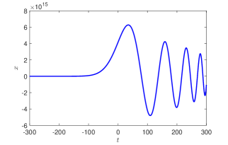
(a) Plot of $x$ vs $t$.

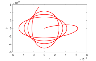
(b) Plot of $\dot{x}$ vs $x$.

Figure 1: Trajectories and phase space diagram solved from Eq.(4.4) with $q=0.1$, $a=0.01=b$,$\alpha_{1}=0.01=\alpha_{2}$, $\Omega=0.01$. The initial conditions are $x(0)=0$, $\dot{x}(0)=0.1$.

In order to study the integrable modulated Mathieu equation (4.1) which leads to a special kind of time-dependent damping, at first we fix

$$\omega^{2}(t)=a+b\cos\Omega t.$$ (4.3)

Since

$$\frac{d}{dt}\left(\frac{\dot{x}}{\omega(t)}\right)+\omega(t)x=\ddot{x}-\frac{\dot{\omega}(t)}{\omega(t)}\dot{x}+\omega^{2}(t)=0,$$

hence the modulated Mathieu equation is given by

$$\ddot{x}+\frac{\Omega b\sin\Omega t}{2(a+b\cos\Omega t)}\dot{x}+a+b\cos(\Omega t)x=0.$$ (4.4)

and set $\omega^{2}(t)=a+b\cos(\Omega t)$. This has a distinct advantage for us, since it is already mentioned in (2.3) that this admits the following first integral, viz

$$I(x,\dot{x},t)=\frac{1}{2}\left[\left(\frac{\dot{x}^{2}}{a+b\cos(\Omega t)}\right)+x^{2}\right].$$ (4.5)

Thus on the level surface $I=C_{1}$ one finds that the general solution of the integrable modulated Mathieu equation, which is given by

$$\int\frac{dx}{\sqrt{2C_{1}-x^{2}}}=\pm\int\sqrt{a+b\cos\Omega t}\;dt+C_{2},$$ (4.6)

with $C_{1}$ and $C_{2}$ being arbitrary constants. Explicit evaluation of the integral on the left yields

$$x(t)=\sqrt{2C_{1}}\sin\left(\pm\int\sqrt{a+b\cos\Omega t}\;dt+C_{2}\right).$$ (4.7)

Note that the integral on the right hand side may be expressed in terms of an elliptic integral of the second kind.

In figure (1), the trajectories and the phase space diagrams are depicted from the modulated Mathiew equation viz. Eq.(4.4). One can see that the periodic oscillation of the system i.e. the $x$ vs $t$ graph is somewhat damping in nature. This solution is analogous to the Airy function viz. $Ai(-t)$ as discussed by Berry[20]. In the limit, $a,b,\Omega\rightarrow 0$, Eq.(4.4) represents analogous $Ai$ function solutions. On the other hand in the phase space diagram the periodic behavior is approached with many periods along with different amplitudes while the time part is changing from some negative finite value to positive finite value. The nature of this phase space is somewhat analogous to the functional plot of $Ai(-t)$ vs $Ai^{\prime}(-t)$. This might be the direct consequence of the Eq.(4.4) under the previously said parametric range. This phase space diagram ensures the trapping of the charged particles within the domain of the periodic boundaries. These lines are not totally the heteroclinic orbits where the system starts from one saddle point and finishes with another saddle points without any kind of periodicity, instead, they are close to limit cycles.

4.1 Damped extension of the nonlinear Mathieu equation

In this section we extend the result of the previous section to a damped counter part of the nonlinear version of the Mathieu equation considered by Abraham and Chatterjee[21]. A weakly nonlinear version of the Mathieu equation is applicable among other things, also to Paul trap mass spectrometers which use static direct current (DC) and radio frequency (RF) oscillating electric fields to trap ions.

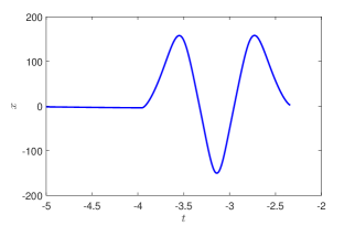
(a) Plot of $x$ vs $t$.

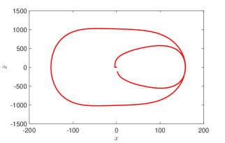
(b) Plot of $\dot{x}$ vs $x$.

Figure 2: Trajectories and phase space diagram solved from Eq.(4.9) with $q=0.1$, $a=0.01$,$\alpha_{1}=0.1=\alpha_{2}$. The initial conditions are $x(0)=0$, $\dot{x}(0)=0.1$.

Consider a nonlinear Mathieu equation of the form

$$\ddot{x}+(a+2q\cos 2t)(x+\alpha_{1}x^{2}+\alpha_{2}x^{3})=0,$$ (4.8)

where the parameters $\alpha_{1}$ and $\alpha_{2}$ are small. We study this nonlinear Mathieu equation in presence of time dependent damping, given by

$$\ddot{x}+\big{(}\frac{2q\sin\,2t}{a+2q\cos\,2t}\big{)}\dot{x}+(a+2q\cos 2t)^{2}(x+\alpha_{1}x^{2}+\alpha_{2}x^{3})=0.$$ (4.9)

In figure (2), we plotted the trajectory and the phase space for the Eq.(4.9). The space part shows a pulse propagation. This solution is also analogous to the Airy function viz. $Ai(-t)$ given by the Eq.(4.9) in the limit $q,a,\alpha_{1},\alpha_{2}\rightarrow 0$.[20] The phase space shows a periodic nature with double periods. The nature can be treated as the homoclinic as the system starts from one saddle point and almost comes back to that point again with the time running from some negative finite value to positive finite value. In the mean time it traces double periodic nature. One thing to notice here that the periods have different amplitudes and the charged particles can almost be trapped inside those two periodic boundaries.

Let us set $\omega(t)=(a+2q\cos\,2t)$, so that we may identify (4.9) with (2.6) for $F(x)=x+\alpha_{1}x^{2}+\alpha_{2}x^{3}$, the corresponding potential function is given by

$$U(x)=\frac{1}{2}x^{2}+\frac{\alpha_{1}}{3}x^{3}+\frac{\alpha_{2}}{4}x^{4}).$$ (4.10)

It is clear from the knowledge of earlier sections that the system (4.9) has a first integral given by

$$I=\frac{1}{2}\Big{[}(\frac{\dot{x}}{\omega(t)})^{2}+(x^{2}+\frac{2\alpha_{1}}{3}x^{3}+\frac{\alpha_{2}}{2}x^{4}\Big{]},$$ (4.11)

where $\omega(t)=\sqrt{a+2q\cos\,2t}$.

4.2 Mathieu-Kapitza equation

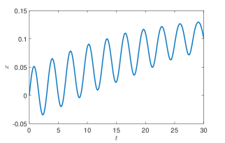
(a) Plot of $x$ vs $t$.

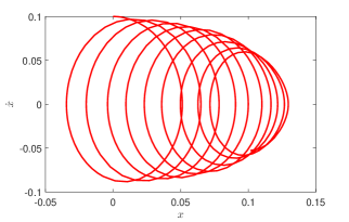
(b) Plot of $\dot{x}$ vs $x$.

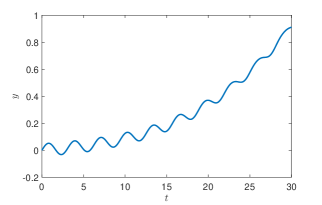
(c) Plot of $y$ vs $t$.

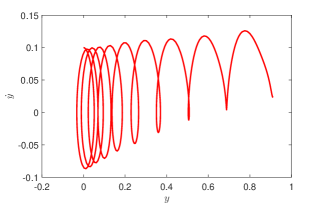
(d) Plot of $\dot{y}$ vs $y$.

Figure 3: Trajectories and phase space diagram solved from Eqs.(4.12,4.13) with $q=0.1$, $a=0.01$. The initial conditions are $x(0)=0$, $\dot{x}(0)=0.1$, $y(0)=0.0$, $\dot{y}(0)=0.1$.

Motivated from the above idea we can give a Mathieu modulation of the Kapitza equation If we substitute $\omega^{2}(t)=(a+2q\cos\,2t)$ in parametric Kapitza equation we obtain

$$\ddot{x}+\big{(}\frac{4q\sin\,2t}{a+2q\cos\,2t}\big{)}\dot{x}+(a+2q\cos 2t)^{2}(x+y)=0,$$ (4.12)

$$\ddot{y}+\big{(}\frac{4q\sin\,2t}{a+2q\cos\,2t}\big{)}\dot{x}-(a+2q\cos 2t)^{2}(x-y)=0.$$ (4.13)

Clearly this pair belongs to the family of coupled linear damped Mathieu equations and the underlying potential is the simple saddle.

The integral of motion of this set of equations are given by

$${\cal I}_{1}=\frac{1}{2}\Big{[}\frac{\dot{x}^{2}}{a+2q\cos\,2t}-\frac{\dot{y}^{2}}{a+2q\cos\,2t}+(x^{2}-y^{2})+2xy\Big{]},$$ (4.14)

$${\cal I}_{2}=\frac{\dot{x}\dot{y}}{a+2q\cos\,2t}-\frac{1}{2}(x^{2}-y^{2})+xy.$$ (4.15)

Similarly we can derive the nonlinear Mathieu-Kapitza equation using the Monkey saddle. Hence using (3.10) we obtain

$$\ddot{x}+\big{(}\frac{2q\sin\,2t}{a+2q\cos\,2t}\big{)}\dot{x}+(a+2q\cos 2t)^{2}\big{(}x^{2}-y^{2}+2xy\big{)}=0,$$ (4.16)

$$\ddot{x}+\big{(}\frac{2q\sin\,2t}{a+2q\cos\,2t}\big{)}\dot{x}-(a+2q\cos 2t)^{2}\big{(}x^{2}-y^{2}-2xy\big{)}=0.$$ (4.17)

In figure (3), we plot the space and phase parts of the dynamical variables $x$ and $y$ for the parametric Kapitza equation viz. Eqs.(4.12,4.13). We can see that both the space parts viz. figures (3(a),3(b)) have periodicity but the amplitudes are inclining with time. The most important observation is the phase space plots viz. figures (3(c),3(d)) of the two variables $x$ and $y$. While we are having periodic cycles for the $x$ with different amplitudes, we get heteroclinic orbits for the other variable $y$. This seems to be very interesting indeed. It is a mixed phase space with both trapping and escaping particles!

5 Outlook

In this paper we have re-examined integrable modulation problem once formulated by Moser and Veselov. We have employed the algorithm given by Bartuccelli and Gentile to construct parametric generalization of Kapitza equation of rotating shaft. It is known that potential of the Kapitza equation is associated to simple saddle and its $\pi/2$ degree form. We generalized the Kapitza equation and its parametric generalization using immediate next higher-order saddle, monkey saddle. We illustrated our construction for $\omega^{2}(t)=a+2q\cos\,2t$ and demonstrated how one can combine the Kapitza equation with the Mathieu equation, which we coined as Mathieu-Kapitza equation. It is noteworthy that the Kapitza family of equation yields curl forces as pointed out by Berry and Shukla. The numerical demonstration of the parametric equations shows various natures of the phase space trajectories and also opens up the novelty in particle trapping. The introduction of the parametric curl forces in different cases, as discussed, shows that the trapping can either be well and truly on the way or it can be escaped from the system. The tuning of the parameter plays a very crucial role in confining such particles and in this sense we argue that out novel findings may play a bigger role in it. In this sense we can say that this paper demonstrated a parametric generalization of the curl force problem which in turn be a very useful in explaining many of the laboratory observations regarding particle trapping. Also the analogous Airy function solutions to the modulated Mathieu equation is another novel finding in this present context. Lastly, by following the methodology proposed by Gibbons and his coworkers, we also provided a geometric description of the integrable modulated oscillator using the Eisenhart-Duval lift.

Declarations

PG thanks Khalifa University for its continued support. SG thanks Diamond Harbour Women’s University for providing the necessary research environment with constant encouragement and support.

Conflicts of interest

None.

Availability of data and material (data transparency)

Not applicable.

References

- [1] M V Berry and P Shukla, Classical dynamics with curl forces, and motion driven by time-dependent flux, J. Phys. A 45 (2012) 305201.
- [2] M V Berry and P Shukla, Hamiltonian curl forces, Proc. R. Soc. A 471 (2015) 20150002 (13pp).
- [3] A.P. Veselov, A few things I learnt from Jürgen Moser, Regular and Chaotic Dynamics 13, 515–524 (2008).
- [4] M V Bartuccelli and G Gentile, On a class of Integrable time-dependent dynamical systems, Phys Letts A 307 (2003), no. 5-6, 274-280.
- [5] M Bartuccelli, G Gentile and J A Wright, On a class of Hill’s equations having explicit solutions, Appl. Math. Lett. 26 (2013) 1026-1030.
- [6] A. Ghose Choudhury and P. Guha, Damped equations of Mathieu type, Appl. Math. Comput. 229 (2014), 85–93.
- [7] P. Guha and A. Ghose Choudhury, Integrable Time-Dependent Dynamical Systems: Generalized Ermakov-Pinney and Emden-Fowler Equations, Nonlinear dyns. systems theory 14 (4) (2014) 355-370.
- [8] P Guha, Saddle in linear curl forces, cofactor systems and holomorphic structure, Eur. Phys. J. Plus 133, 536 (2018).
- [9] P Guha, Curl forces and their role in optics and ion trapping, Eur. Phys. J. D 74, 99 (2020).
- [10] S. Garai and P. Guha, Higher-order saddle potentials, nonlinear curl forces, trapping and dynamics, Nonlinear Dyn (2021), https://doi.org/10.1007/s11071-021-06212-w
- [11] P L Kapitsa, Stability and transition through the critical speed of fast rotating shafts with friction . Zhur. Tekhn. Fiz. 9 (1939) 124-147.
- [12] D R Merkin, Gyroscopic systems, Nauka, Moscow, in Russian (first edition - 1956) 1974.
- [13] D R Merkin, Introduction to the theory of stability, 1997 Springer-Verlag, New York.
- [14] L. Righetti, J. Buchli and A. Ijspeert, Dynamic hebbian learning in adaptive frequency oscillators, Physica D 216 (2006) 269-281.
- [15] L. P. Eisenhart, Dynamical trajectories and geodesics, Annals Math.30 (1929) 591.
- [16] C. Duval, G. Burdet, H. Künzle, M. Perrin, Bargmann structures and Newton–Cartantheory, Phys. Rev. D31 (1985) 1841
- [17] C. Duval, G.W. Gibbons, P.A. Horvathy, Celestialmechanics, conformal structures and gravitational waves, Phys. Rev. D43 (1991) 3907.
- [18] M. Cariglia, A. Galajinnsky, G. W. Gibbons, P. A. Horvathy, Cosmological aspects of the Eisenhart-Duval lift, Eur. Phys. J. C(2018) 78: 314.
- [19] F. M. Arscott, The Whittaker-Hill equation and the wave equation in paraboloidal co-ordinates, Proc. Roy. Soc. Edinburgh Sect. A 67 (1967) pp. 265–276.
- [20] M. V. Berry, Classical and quantum complex Hamiltonian curl forces, J. Phys. A: Math. Theor. 53, 415201 (2020).
- [21] G. T. Chatterjee and A. Chatterjee, Approximate asymptotics for a nonlinear Mathieu equation using harmonic balance based averaging, Nonlinear Dyn. 31(4), 347-365 (2003).