Probing Negative Sampling Strategies to Learn Graph Representations via Unsupervised Contrastive Learning

Abstract

Graph representation learning has long been an important yet challenging task for various real-world applications. However, their downstream tasks are mainly performed in the settings of supervised or semi-supervised learning. Inspired by recent advances in unsupervised contrastive learning, this paper is thus motivated to investigate how the node-wise contrastive learning could be performed. Particularly, we respectively resolve the class collision issue and the imbalanced negative data distribution issue. Extensive experiments are performed on three real-world datasets and the proposed approach achieves the SOTA model performance.

1 Introduction

In the literature, various graph neural network (GNN) models have been proposed for graph analysis tasks, such as node classification [14], link prediction [35] and graph classification [33]. Generally, most existing GNN-based approaches are proposed to train, in a supervised manner, graph encoder to embed localized neighboring nodes or node attributes for a graph node into the low-dimensional feature space. By convoluting $K$-hops neighboring nodes, adjacent nodes naturally have similar feature representations. Notably, the consequent downstream tasks inevitably rely on the quality of the learnt node embeddings.

For many real graph applications, e.g., protein analysis [37], it intuitively requires an unavoidable cost or even the specialized domain knowledge to manually annotate sufficient data to well train the graph encoders by minimizing the loss associated with the specified supervised learning task. Alternatively, a number of milestone unsupervised random walk based GNNs, including but not limited to node2vec [8] and graph2vec [21], are consequently proposed towards training the universal node embeddings and then various supervised downstream tasks are directly applied on these node embeddings. Similarly, another line of unsupervised graph representation learning approaches, i.e., graph kernel based methods, also utilizes the graph structural information to embed graph nodes with similar structures into similar representations. Most recently, the contrasive learning [11, 12] is originally proposed to learn feature embeddings for each image in a self-supervised manner. To this end, these proposed approaches first generate two random augmentations for the same image and define these two as a pair of positive samples, and simply treat samples augmented from other images as negative samples. Then, the contrastive loss is designed to maximize the mutual information between each pair of positive samples. The learnt embeddings are believed to well preserve its inherent discriminative features. Research attempts are then made to adapt the successful contrastive learning approaches to unsupervised graph representation learning problem [10, 30]. In [30], the graph-level representation is built to contrast with each node representation to acquire node representations fitting for diverse downstream tasks. [10] adopts diffusion graph as another view of the given graph, and the contrast is performed between graph representation of one view and node representation of another view. As all the node embeddings are forced to approximate the same graph representation. Intuitively, a coarser level graph analysis task, e.g., graph classification, would benefit a lot from such kind of contrastive learning, whereas a fine-grained level task, e.g., node classification, might not benefit that large.

To address aforementioned research gap, this work is thus motivated to investigate whether the contrastive learning could be effectively carried on in a node-wised manner. That is, for each graph node $x$ to be embedded, our desired contrastive learning is to maximize the mutual information between $x$ and its positive examples $x^{+}$ instead of a graph representation, and simultaneously to minimize the mutual information between $x$ and its negative examples $x^{-}$. Meanwhile, there exist two research challenges to be addressed. First, the sampled negative examples $x^{-}$ might contain the true positive example $x^{+}$ which is known as class collision issue. Second, how the density of negative samples will affect the contrastive learning has not been studied. We assume that the underlying true positive examples could be statistically similar to $x$, i.e., unseen positive examples should obey the same prior probability distribution as $x$. Similarly, the multiple typed negative examples $x^{-}$ are assumed to obey different probability distributions. With this assumption, the class collision issue could be intuitively resolved by removing those examples from the set of $x^{-}$ they are more likely generated by the assumed positive data distribution. For the second point, it can be known from the contrasitive loss that $x$ will be farther away from feature area with dense $x^{-}$ than area with sparse $x^{-}$. The density distribution of $x^{-}$ is used as factor to determine the distance of $x$ and $x^{-}$ is questionable. Therefore, after removing negative examples in doubt, a subset of negative examples should be diversely sampled to form $x^{-}$ for the contrastive learning. Thus, this paper proposed an adaptive negative sampling strategy for the learning of the node embedding in a node-wised contrastive learning manner. The major contribution of this paper are summarized as follows.

• To the best of our knowledge, this paper is among the first attempts to propose a node-wise contrastive learning approach to learn node embedding in an unsupervised manner. In the proposed approach, positive samples and negative samples are assumed to obey different data distributions, and the class collision issue could be addressed by eliminating in doubt negative samples if they are more likely generated by a positive data distribution.

• We propose a determinantal point process based negative instances sampling strategy which is believed to be able to sample diverse negative examples to be contrasted to learn node embedding.

• We perform extensive experiments on several benchmark datasets and the promising results have demonstrated that the proposed approach is superior to both baseline and the state-of-the-art approaches.

The rest of this paper is organized as follows. Section 2 reviews related work and then we formulate the problem in Section 3. The proposed approach is detailed in Section 4. Experimental results are reported in Section 5 and we conclude the paper in Section 6.

2 Related Work

2.1 Graph Representation Learning

2.1.1 Supervised Methods

The earlier graph representation learning attempts have been made in the supervised settings. ChebyNet [4] and GraphWave [31] leverage graph Fourier transformations to convert graph signals into spectral domain. Kipf and Welling [14] propose graph convolutional network (GCN) via a localized first-order approximation to ChebyNet [4], and extend graph convolution operations to the aggregation of neighbor nodes. To further the success of GCN, GAT [29] and GeniePath [16] are proposed to sample more informative neighbor nodes for the convolutions. There also exist some approaches targeting at resolving efficiency issue [9, 3].

2.1.2 Unsupervised Methods

The unsupervised graph representation learning methods could be classified into random walk-based methods [28, 23] and graph kernel-based methods [2, 26]. The random walk-based methods are applied for each graph node and the nodes in a sequence of walk are to be encoded. By dosing so, the neighboring nodes generally are trained to have similar embeddings regardless of the graph structural information as well as the node attributes. Such kinds of methods are usually transductively performed and thus need to be re-trained to represent the unseen nodes which inevitably limits their wide applicability.

2.2 Contrastive Learning and Negative Sampling

Contrastive learning is recently proposed to learn feature embeddings in a self-supervised manner. The quality of the learnt embeddings largely replies on the generated positive instance set and the negative instance set. Accordingly, various approaches have been proposed with a focus on constructing positive samples. In the domain of NLP, [17] treats the contextual sentences as positive pairs. For the domain of image recognition, a good number of research works are proposed to train encoders to discriminate positive samples from negative samples. For graph data, [8] encodes graph nodes using a generalized proximity and treats these nodes not appearing in $w$ steps of a random walk or without common neighbors as negative examples. In [25], two nodes that have a similar local structure are considered as positive sample pairs despite the node position and its attributes. Then, several SOTA approaches have been proposed to adapt contrastive learning on graph data [30, 27, 10, 24]. DGI [30] maximizes the mutual information between the node embeddings and graph embeddings.

InfoGraph [27] treats nodes that are virtually generated by shuffling feature matrix as negative samples. Mvgrl [10] further defines two views on graph data and graph encoders are trained to maximize mutual information between node representations of one view and graph representations of another view and vice versa. [24] consider two subgraphs augmented from the same $r$-ego network as a positive instance pair and these subgraphs from different $r$-ego as negative sample pair, where $r$-ego represents the induced subgraph containing the set of neighbor nodes of a given node $v$ within $r$ steps.

3 Preliminaries and Problem Formulation

In this section, we first briefly review the Determinantal Point Process (DPP) [18] adopted to diversely sample negative instances, then we describe the notations as well as the problem setup.

3.1 Determinantal Point Process

The original DPP is to proposed to model negatively correlated random variables, and then it is widely adopted to sample a subset of data where each datum in this set is required to be correlated with the specified task, and simultaneously is far away from each other. Formally, let $\mathcal{P}$ denote a probability distribution defined on a power set $2^{Y}$ of a discrete finite point set $Y$ = {$1,2,...,M$}. $Y\sim\mathcal{P}$ is a subset composed of data items randomly generated from $\mathcal{P}$. Let $A$ be a subset of $Y$ and $B\in\mathbb{R}^{M\times M}$ be a real positive semi-definite similarity matrix, then we have

$$\mathcal{P}(A\subseteq Y)=|B_{A}|,$$ (1)

where $B_{A}$ is a sub-matrix of $B$ indexed by the elements of subset $A$. $|\cdot|$ denotes the determinant operator. If $A=\{i\}$, $\mathcal{P}(A\subseteq Y)=B_{i,i}$; and if $A=\{i,j\}$, $\mathcal{P}(A\in Y)$ can be written as

$$\mathcal{P}(A\subseteq Y)=\begin{vmatrix}B_{i,i}&B_{i,j}\\ B_{j,i}&B_{j,j}\end{vmatrix}=\mathcal{P}(i\in Y)\mathcal{P}(j\in Y)-B_{i,j}^{2},$$ (2)

Thus, the non-diagonal matrix entries represent the correlation between a pair of data items. The larger the value of $B_{i,j}$, the less likely that $i$ and $j$ appear at the same time. Accordingly, the diversity of entries in the subset $A$ could be calculated. As for our approach, DPP is adapted to sample a evenly distributed subset from negative instance set.

3.2 Notations and Definitions

Let $G=(V,E)$ denote a graph, $V$ denote the node set containing $N$ nodes, $E\subseteq V\times V$ denote the edge set where $e=(v_{i},v_{j})\in E$ denotes an edge between two graph nodes, $\mathrm{X}=\{x_{1},...,x_{d}\}$ denote the node feature set where $x_{i}\in\mathbb{R}^{d_{in}}$ represents the features of node $v_{i}$. The adjacency matrix is denoted as $\mathrm{A}\in\mathbb{R}^{N\times N}$, where $\mathrm{A}_{ij}=1$ represents that there is an edge between $v_{i}$ and $v_{j}$ in the graph and 0 otherwise. For a given node $v_{i}$, its $K$-hops neighbor set is denoted as $\mathcal{N}_{K}(v_{i})$ containing all neighboring nodes of $v_{i}$ within $K$ hops, defined as $\mathcal{N}_{K}=\{v_{j}:d(v_{i},v_{j})\leq K\}$ where $d(v_{i},v_{j})$ is the shortest path distance between $v_{i}$ and $v_{j}$ in the graph $G$. Then, the induced subgraph is defined as follows.

Definition 1

Induced subgraph $s$. Given $G=(V,E)$, a subgraph $s=(V^{\prime},E^{\prime})$ of $G$ is said to be an induced subgraph of $G$ if all the edges between the vertices in $V^{\prime}$ belong to $E^{\prime}$.

3.3 Problem Setup

Given a $G$, our goal is to train a graph encoder $\mathcal{G}:\mathbb{R}^{N\times F}\times\mathbb{R}^{N\times N}\to\mathbb{R}^{N\times d}$, such that $\mathcal{G}(\mathrm{X},\mathrm{A})=\mathrm{H}=\{h_{1},...,h_{N}\}$ represents the low-dimensional feature representations, where $h_{i}$ denotes the embeddings of $v_{i}$. Then, the learnt $\mathcal{G}$ is used to generate node embeddings for downstream tasks, e.g. node classification.

The purpose of our approach is to maximize the mutual information between a pair of positive instances, and minimize the mutual information between a pair of negative and positive instances simultaneously. Similar to the infoNCE [22], the general form of our unsupervised contrastive learning is to minimize the contrastive loss, given as

$${L}=-\sum_{i=1}^{N}\log\frac{e^{f({h}_{i}^{q},{h}_{i}^{k})/\tau}}{e^{f({h}_{i}^{q},{h}_{i}^{k})/\tau}+\sum_{j\not=i}^{N}e^{f({h}_{i}^{q},{h}_{j}^{k})/\tau}},$$ (3)

where $f(\cdot,\cdot)$ is the score function to score the agreement of two feature embeddings, and in our approach the score function is simply the dot product calculated as $f({h}_{i}^{q},{h}_{j}^{k})=h_{i}^{q}\cdot{h_{j}^{k}}^{T}$, and $\tau$ is the temperature hyper-parameter. $h_{i}^{k}$ is a positive instance of $h_{i}^{q}$ , and two of them are usually defined as two different random augmentations of the same data. In our model, we define $h_{i}^{q},h_{i}^{k}$ are two random augmented embeddings of $v_{i}$. Note that the first term of the denominator is to maximize the mutual information between a pair of positive instances, and the second term is to minimize the mutual information between a pair of negative and positive instances. By optimizing Eq. 3, the employed model is believed to be able to learn the most discriminative features that are invariant to positive instances.

Nevertheless, there are some problems to be address. Intuitively, we hope that two nodes that have the same label in the downstream task should have similar embeddings. However, we treat $h_{j\not=i}^{k}$ as negative sample and try to be away from it in feature space while $v_{j}$ may have the same label as $v_{i}$, which is called class collision. At the same time, we noticed that the current negative sampling strategy ignores the influence of the density of embedding distribution of negative samples. A node embedding will be updated to be farther away from feature subspace where its negative nodes are more densely distributed. Therefore, we designed approach to adaptive sampling negative samples to avoid those problems described above.

4 The Proposed Approach

4.1 Graph Embeddings

The proposed node-wised contrastive learning scheme allows various choices of the graph neural network architectures. We opt for simplicity reason and adopt the commonly adopted graph convolution network (GCN) [14] as our graph encoder $\mathcal{G}$.

4.1.1 Augmentation

By following [24], we first employ a $k$-steps random walk on $G$ starting from a specific node $v_{i}$, and a sequence of walking nodes $seq_{i}$ = {$t_{1},...,t_{k}$} is used to form the set of vertices $V^{\prime}$. The subgraph $s_{i}$ induced by $V^{\prime}$ is regarded as a random augmentation of node $v_{i}$. Then, we repeat aforementioned procedure and eventually we generate two induced subgraphs $s_{i}^{q},s_{i}^{k}$, those embeddings are respectively denoted as $h_{i}^{q}$ and $h_{i}^{k}$ and regarded as a positive pair.

4.1.2 Encoder

The employed GCN layers are defined as $\sigma(\widetilde{\mathrm{A}}_{i}\mathrm{X}_{i}W)$ which is used to embed node $v_{i}$, where $\widetilde{\mathrm{A}}_{i}={\widehat{\mathrm{D}}_{i}}^{-\frac{1}{2}}\widehat{\mathrm{A}}_{i}{\widehat{\mathrm{D}}_{i}}^{-\frac{1}{2}}\in\mathbb{R}^{n_{i}\times n_{i}}$ is symmetrically normalized adjacency matrix of a subgraph $s_{i}$. $\widehat{\mathrm{D}}_{i}$ is the degree matrix of $\widehat{\mathrm{A}}_{i}={\mathrm{A}}_{i}+\mathrm{I}_{n_{i}}$, where ${\mathrm{A}}_{i}$ is the original adjacency matrix of $s_{i}$, $\mathrm{X}_{i}\in\mathbb{R}^{n_{i}\times d}$ is the initial features of nodes in $s_{i}$, $W\in\mathbb{R}^{d_{in}\times d}$ is network parameters, $\sigma$ is a ReLU [7] non-linearity and $n_{i}$ is the number of nodes contained in $s_{i}$. Putting $\widetilde{\mathrm{A}}_{i},\mathrm{X}_{i}$ into graph layer to perform convolution operation and then we could acquire node embeddings $H_{i}\in\mathbb{R}^{n_{i}\times d}$ of subgraph $s_{i}$.

4.1.3 Readout

After convolution operation of GNN layers, we feed the embedding set $H_{i}$ into the readout function $\mathcal{R}(\cdot)$ to compute an embedding of $v_{i}$. The readout function adopted in the experiments is given as follows

$$\mathcal{R}(H_{i})=\sigma(\frac{1}{n_{i}}\sum_{j=1}^{n_{i}}h_{i,j}+\max(H_{i})),$$ (4)

where $h_{i,j}$ represents the $j$-th node embedding in $H_{i}$, $\max(\cdot)$ simply takes the largest vector along the row-wise and $\sigma$ is the non-linear sigmoid function. Eventually, the node embedding is acquired as $h_{i}=\mathcal{R}(H_{i})$. The node encoding process is illustrated in Algorithm 1.

Input: graph $G$, adjacency matrix $\mathrm{A}$, feature matrix $\mathrm{X}$,

graph encoder $\mathcal{G}$, score function $f$, readout function $\mathcal{R}$,

random-walk operator $\mathcal{RW}$, subgraph sampler $\Gamma_{sub}$, concatenator $\parallel$

Output: The node embeddings $\mathrm{H}^{q}\in\mathbb{R}^{N\times d},\mathrm{H}^{k}\in\mathbb{R}^{N\times d}$

1 Initialize $\mathrm{A}$ and $\mathrm{X}$;

2

3for  i=1 to $N$ do

4       $s_{i}^{q}$ = $\mathcal{RW}(v_{i})$, $s_{i}^{k}$ = $\mathcal{RW}(v_{i})$

5       $\mathrm{A}_{i}^{q},\mathrm{X}_{i}^{q}$ = $\Gamma_{sub}(s_{i}^{q},\mathrm{A},\mathrm{X})$

6       $\mathrm{A}_{i}^{k},\mathrm{X}_{i}^{k}$ = $\Gamma_{sub}(s_{i}^{k},\mathrm{A},\mathrm{X})$

7       $H_{i}^{q}$ = $\mathcal{G}(\mathrm{A}_{i}^{q},\mathrm{X}_{i}^{q})$, $H_{i}^{k}=\mathcal{G}(\mathrm{A}_{i}^{k},\mathrm{X}_{i}^{k})$

8       $h_{i}^{q}=\mathcal{R}(H_{i}^{q})$, $h_{i}^{k}=\mathcal{R}(H_{i}^{k})$

9      

10 end for

11return $\mathrm{H}^{q}$ = $\mathop{\big{\|}}\limits_{i=1}^{N}h_{i}^{q}$, $\mathrm{H}^{k}$ = $\mathop{\big{\|}}\limits_{i=1}^{N}h_{i}^{k}$

Algorithm 1 Generate embeddings of the augmented instances

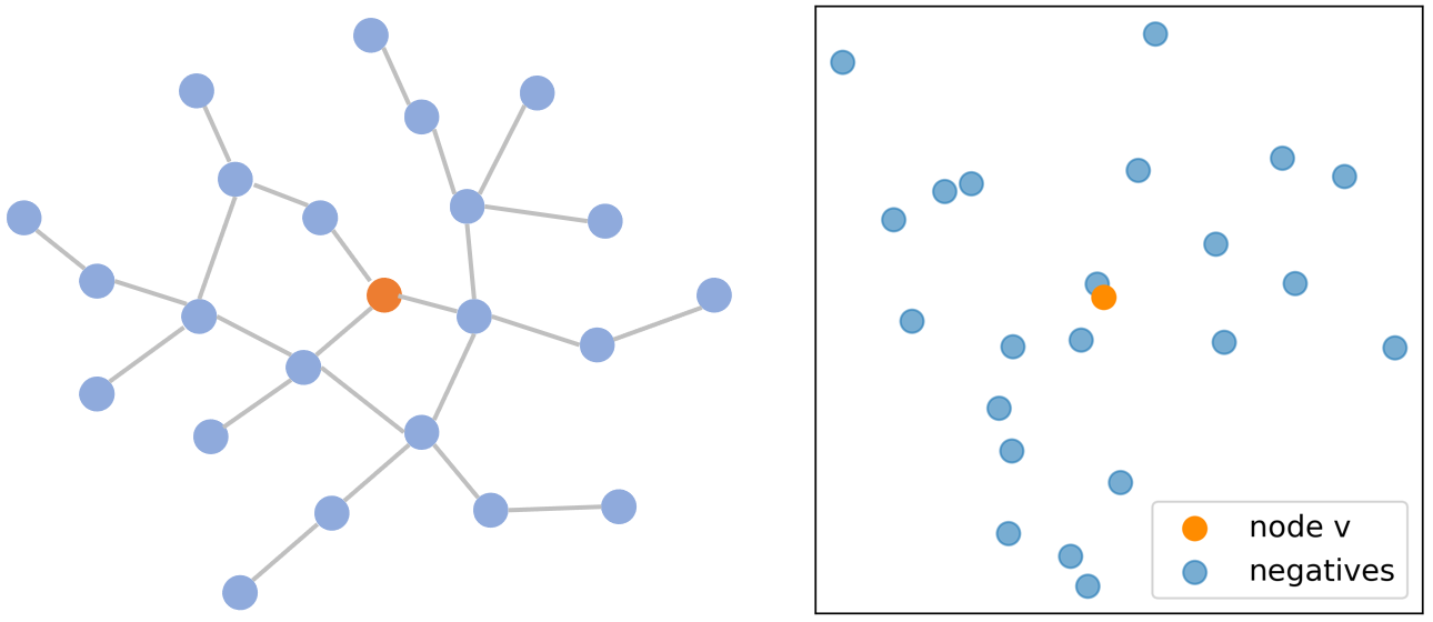
(a) Initial stage: target node $v$ (in red).

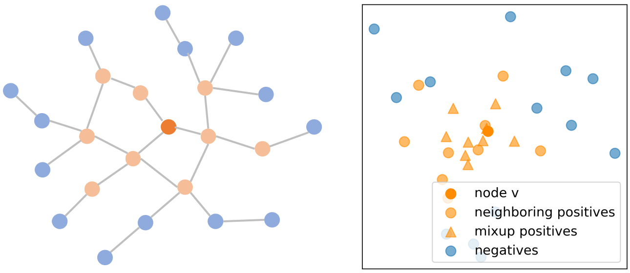
(b) The augmented positive instances.

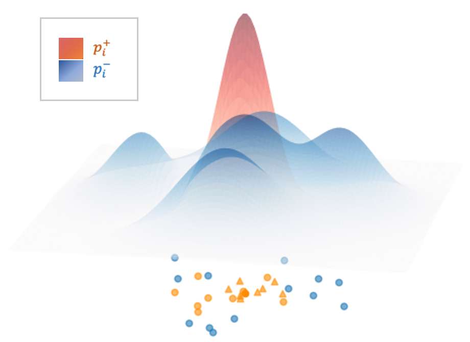
(c) Fit the embedding distribution for positive and negative samples.

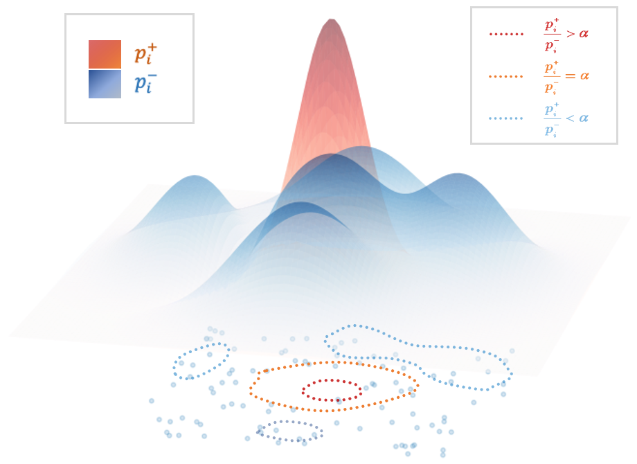
(d) Resample the negative samples.

Figure 1: Process of generating positive and negative samples by our approach. In each subfigure, the left depicts the graph topological structure and the right plots the feature embedding space where each colored dot represent the embeddings of a positive or negative data node. In the initial stage, plotted in (a), there is only one target node treated as positive node (in red) and the rest are negative nodes (in blue). In (b), the positive nodes are augmented by adding “in-doubt” nodes (in orange dot) and mixup positive nodes (in orange triangle), and from the right figure, it is noticed that the embeddings of orange dots and triangles are close to that of the target node (red dot). And orange and blue nodes could be well separated which indicates two distributions could be estimated. In (c), the underlying positive instance distribution and negative instance distribution could be well fit using these data. In (d), the dashed loop is the contour of $\frac{p_{i}^{+}(v_{j})}{p_{i}^{-}(v_{j})}$. Note that the smaller the orange dashed loop, the more confident that datum falling a positive instance.

4.2 Resolving Class Collision

Given a node $v_{i}$, its negative and positive sample set are respectively denoted as $S_{i}^{-}=\{v_{1},...,v_{i-1},v_{i+1},v_{N}\}$ and $S_{i}^{+}=\{v_{i}\}$. To alleviate the class collision issue, it is desired to discover those “in doubt” negative samples that are more likely to belong to the same class of $v_{i}$. The overall procedure is depicted as below.

First, we assume that $S_{i}^{+}$ and $S_{i}^{-}$ respectively obey different prior probability distributions. The “in-doubt” negative examples are discovered if they are more likely to be generated by the data distribution of positive instances. To fit the embedding distribution $p_{i}^{+}$ and $p_{i}^{-}$, we employ two independent neural networks, i.e., $\mathcal{F}_{i}^{+}$ and $\mathcal{F}_{i}^{-}$ to fit the distributions. If the probability that $v_{j}$ belongs to $S_{i}^{+}$ is higher than the probability of being a negative instance, i.e., $\frac{p_{i}^{+}(v_{j})}{p_{i}^{-}(v_{j})}>\alpha$, we remove $v_{j}$ from $S_{i}^{-}$, where $\alpha$ is the soft-margin to discriminate an instance. Detailed steps are illustrated in the following paragraphs.

4.2.1 Forming the sample set $S_{i}^{+}$ and $S_{i}^{-}$

Initially, the positive instance of a given node $v_{i}$ is also augmented by $v_{i}$ plotted in orange and the rest nodes plotted in light-blue are considered as negative instances, which is shown in Figure 1(a). Apparently, not all the blue data are the true negative instances. To consider the unsupervised settings, it is acceptable to assume that the “closest” node to $v_{i}$ should have the same underlying class label. Therefore, a few nearest neighbor nodes $v_{j}\in\mathcal{N}_{K}$ are transited to $S_{i}^{+}$ from $S_{i}^{-}$. Using the mixup algorithm [34], more positive samples will be generated to further augment the positive instance set $S_{i}^{+}$. and the results are illustrated in Figure 1(b).

4.2.2 Fitting the positive and negative instance distribution

With the augmented $S_{i}^{+}$ and $S_{i}^{-}$, we employ two independent two neural networks $\mathcal{F}_{i}^{+}$, $\mathcal{F}_{i}^{-}$ to respectively fit the embeddings distribution for $v\in S_{i}^{+}$ and $v\in S_{i}^{-}$ as plotted in Figure 1(c). To train $\mathcal{F}_{i}^{+}$, we treat it as a classifier, and data belong to $\mathcal{S}_{i}^{+}$ is assigned with a virtual label $class$ $1$, and data belong to $\mathcal{S}_{i}^{-}$ is virtually assigned with $class$ $0$. On the contrary, to train $\mathcal{F}_{i}^{-}$, we will assign label $class$ $1$ to the data belonging to $\mathcal{S}_{i}^{-}$ and assign label $class$ $0$ to the data belonging to $\mathcal{S}_{i}^{+}$.

For a node $v_{j}\in S_{i}^{-}$, the output of $\mathcal{F}_{i}^{+}(h_{j}^{k})$ and $\mathcal{F}_{i}^{+}(h_{j}^{k})$ are respectively the probability that $v_{j}$ is a positive or negative instance of $v_{i}$. The ratio of these two probabilities with a soft-margin, calculated as $\frac{p_{i}^{+}(v_{j})}{p_{i}^{-}(v_{j})}>\alpha$, is adopted to determine whether $v_{j}$ should be removed from $S_{i}^{-}$ or not, and this soft-margin is plotted in the small orange dashed circle as shown in Figure 1(d).

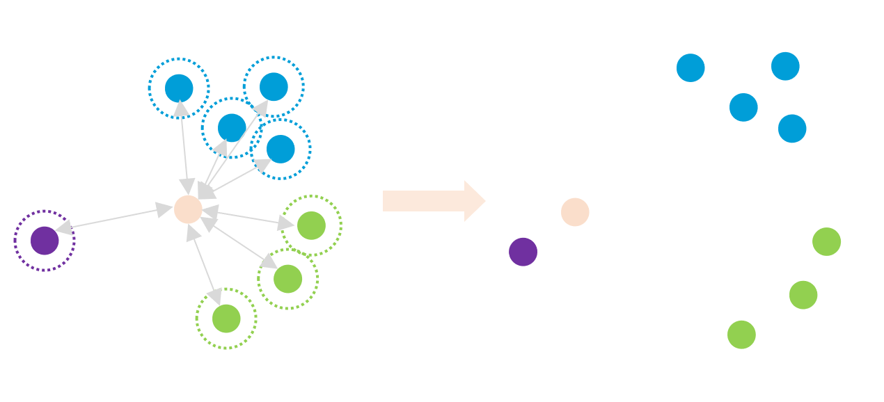
(a) Unevenly sampled negative instances.

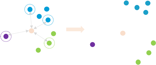
(b) Diversely sampled negative instances.

Figure 2: The illustration of the effect of different sampling strategies. The dashed circle denotes that the corresponding node will be sampled. The pink colored dot is the embedding of target node $v$. (a) shows that for a current strategy, using all negatives, the learnt embeddings of $v$ will close to purple node whereas we desire that the embeddings of $v$ should, simultaneously, stay away from all negative instances as much as possible, as plotted in (b) where a diverse sampling strategy is applied, i.e. the proposed DPP strategy, on the embeddings space and reasonably ignores their distribution.

1

Input: Adjacency matrix $\mathrm{A}$, node embeddings $\mathrm{H}^{q}$, $\mathrm{H}^{k}$,

hyper-parameter $K$, hyper-parameter $\alpha$,

$K$-hops neighbor node set {$\mathcal{N}_{K}(v_{1}),...,\mathcal{N}_{K}(v_{N})$},

DPP sampler $\Gamma_{dpp}$, mixup operator $Mix$,

node embedding set $S$ = {$h_{1}^{k},...,h_{N}^{k}$},

neural network set $\mathcal{F}^{+}=\{\mathcal{F}_{1}^{+},...,\mathcal{F}_{N}^{+}$}, $\mathcal{F}^{-}=\{\mathcal{F}_{1}^{-},...,\mathcal{F}_{N}^{-}$}.

Output: Positive samples sets {$S_{1}^{+},...,S_{N}^{+}$},

negative samples sets {$S_{1}^{-},...,S_{N}^{-}$}.

2 initialization;

3 for i = 1 to $N$ do

4       $S_{i}^{-}$ = $S\setminus\{h_{i}^{k},i\in\mathcal{N}_{K}(v_{i})\}$

5       $S_{i}^{+}$ = $\{h_{i}^{k},i\in\mathcal{N}_{K}(v_{i})\}$

6       $S_{i}^{+}$ = $Mix(S_{i}^{+})$

7      

8 end for

9for i = 1 to $N$ do

10       $p_{i}^{-}$ = $\mathcal{F}_{i}^{-}(S_{i}^{-})$

11       $p_{i}^{+}$ = $\mathcal{F}_{i}^{+}(S_{i}^{+})$

12       for  j = 1 to $N$ do

13             if $j\notin\mathcal{N}_{K}(v_{i})$ and $\frac{p_{i}^{+}(v_{j})}{p_{i}^{-}(v_{j})}>\alpha$ then

14                   $S_{i}^{-}$ = $S_{i}^{-}\setminus\{h_{j}^{k}\}$,

15                   $S_{i}^{+}$ = $S_{i}^{+}\cup\{h_{j}^{k}\}$

16                  

17             end if

18            

19       end for

20      $S_{i}^{-}$ = $\Gamma_{dpp}(S_{i}^{-})$

21 end for

return {$S_{1}^{+},...,S_{N}^{+}$}, {$S_{1}^{-},...,S_{N}^{-}$}

Algorithm 2 Generating positive instance set and negative instance set

4.3 Sampling Diverse Negative Examples

As illustrated in Fig 2, we can regard the process of contrastive learning as the interaction of forces between positive and negative samples. For the worst case of using all instances in $S_{i}^{-}$ for comparison, where the embedding distribution is seriously imbalanced as Fig 2(a), the updated $h_{i}$ will be farther away from the feature subspace where negative samples densely distributed. Intuitively, the comparison result between positive and negative samples should not be related to the density of negative samples. To cope with this distorted updata result, we adapt the Determinant point process (DPP) [18] to our problem. In Fig. 2(b), the DPP algorithm is applied to $S^{-}$ to sample a negative instances subset, where sampled negative instances spread across the entire feature space. In this case, the node embedding can avoid the influence of the density of feature space and be evenly away from each negative sample. We set the correlation between $h_{i}^{q}$ and each negative instance in $S_{i}^{-}$ is equally set to a constant. To calculate the similarity between negative instances, the Euclidean distance is adopted to measure the pair-wise distance, computed as $d(h_{i}^{q},h_{j}^{k})=\sqrt{\sum_{l=1}^{d}({h_{i,l}^{q}}-{h_{j,l}^{k}})^{2}}$.

4.4 Node-wise Contrastive Learning Loss

As pointed in [12], different nodes contribute differently to the unsupervised contrastive learning. We are therefore inspired to further differentiate the importance of the diversely sampled negative instances to our node-wise contrastive learning. For those negative instances that are far away from the query instance $h_{i}^{q}$, the contributions of these nodes are rather limited as they could be easily distinguished w.r.t. $h_{i}^{q}$. However for those close negative instances, it is hard for the model to discriminate them and thus their contributions should be assigned with higher weights.

Accordingly, the weight of the $j$-th negative instance’s embedding $h_{j}^{k}$ w.r.t. the $i$-th positive instance’s embeddings $h_{i}^{q}$ is calculated as $w_{i,j}={h_{i}^{q}\cdot h_{j}^{k}}/\tau_{w}$, where $\tau_{w}$ is a temperature hyper-parameter. Thus, the overall node-wise contrastive loss could be written as

$${L}=-\sum_{i=1}^{N}\log\frac{e^{f({h}_{i}^{q},{h}_{i}^{k})}}{e^{f({h}_{i}^{q},{h}_{i}^{k})}+\sum_{j\in S_{i}^{-}}w_{i,j}e^{f({h}_{i}^{q},h_{j}^{k})}}.$$ (5)

5 Experimental Results

In this section, we first briefly introduce experimental datasets, evaluation metrics as well as the experimental settings. Then, to evaluate the model performance, we not only compare ours method with unsupervised models, but also some supervised models to fully demonstrate the effectiveness of our approach. Extensive experiments are evaluated on several real-world datasets to answer following research questions:

• RQ1: Whether the proposed approach outperforms the state-of-the-art supervised and unsupervised methods or not?

• RQ2: Whether the proposed components could affect the model performance or not (ablation study)?

• RQ3: Whether the proposed approach is sensitive to model parameters or not?

• RQ4: The visualization results of the learnt item embeddings.

5.1 Experimental Setup

5.1.1 Datasets

In the experiments, three widely adopted real-world datasets are adopted to evaluate the model performance including $Cora$ [19], $Citeseer$ [5] and $Pubmed$ [20]. We follow the work [29] to partition each dataset into training set, validation set and test set. The statistics of these datasets are reported in Table 1.

Dataset	# of Nodes	# of Edges	# of Features	# of Classes
Core	2708	5429	1433	7
Citeseer	3327	4732	3703	6
Pubmed	19717	44338	500	3

Table 1: The statistics of experimental datasets.

5.1.2 Baseline models

To evaluate the model performance of the proposed approach on node classification task, both the unsupervised and supervised methods are compared in the experiments.

Available data	Method	Cora	Citeseer	Pubmed
X,Y	Raw features	55.1%	46.5%	71.4%
A,Y	LP	68.0%	45.3%	63.0%
X,A,Y	GCN	81.5%	70.3%	79.0%
X,A,Y	Chebyshev	81.2%	69.8%	74.4%
X,A,Y	GAT	83.0%	72.5%	79.0%
X,A,Y	GeniePath	75.5%	64.3%	78.5%
X,A,Y	JK-Net	82.7%	73.0%	77.9%
X,A,Y	MixHop	81.9%	71.4%	80.8%
A	Deepwalk	67.2%	43.2%	65.3%
X,A	Deepwalk+features	70.7%	51.4%	74.3%
X,A	GAE	71.5%	65.8%	72.1%
X,A	GraphSAGE	68.0%	68.0%	68.0%
X,A	DGI	82.3%	71.8%	76.8%
X,S	DGI	83.8%	72.0%	77.9%
X,A,S	Mvgrl	86.8%	73.3%	80.1%
X,A	ours w/o all	83.5%	69.3%	80.6%
X,A	ours	84.3%	73.5%	81.5%

Table 2: The average node classification results for both supervised and unsupervised models. The available data column highlights the data available to each model during the model training process (X:features, A:adjacency matrix, S:diffusion matrix, Y:labels).

The unsupervised models we used in the experiment are as follows

• Deepwalk [23] first samples related nodes via a truncated random walk, and then constructs negative examples to learn node embeddings. This approach is considered as the baseline method. We also compare our results to DeepWalk with the features concatenated, denoted as DeepWalk+features.

• GAE [15] is considered as the SOTA approach which applies variational auto-encoder to graphs firstly.

• GraphSAGE [9] is proposed to learn a function for generating low-dimensional embeddings by aggregating the embeddings of more informative neighbor nodes. We use the unsupervised loss function mentioned in [9] to train the model.

• DGI [30] is considered as the SOTA unsupervised learning approach which maximizes the mutual information between the node-level and the graph-level feature embeddings.

• Mvgrl [10] is the SOTA self-supervised method proposed to learn node level embeddings by optimizing the contrast between node representations and view-level graph representations.

The semi-supervised models we used in the experiment are as follows

• LP [36] assigns labels to unlabeled samples and is considered as a baseline method.

• GCN [14] is one of the milestone GNN models originally proposed for node classification problem. And the model is trained by minimizing the supervised loss.

• Chebyshev [4] designs the convolution kernels using the Chebyshev inequality to speed up the Fourier transformation for the graph convolution process, and is considered as the baseline.

• GAT [29] is essentially an attention based approach. GAT designs a multi-head self-attention layer to assign weights to different feature embeddings of graph nodes, and is also treated as the baseline.

• GeniePath [16] samples neighboring nodes which contribute a lot to the target node via a hybrid of BFS and DFS search strategy.

• JK-Net [32] adaptively uses different neighborhood ranges for each node to perform aggregation operations.

• MixHop [1] proposes to perform multi-order convolution to learn general mixing of neighborhood information.

5.1.3 Setting of Model Parameters

Our task is to first train the node embeddings and then directly evaluate its node classification ability. We set the same experimental settings as the SOTA [30, 10] and report the mean classification results on the testing set after 50 runs of training followed by a linear model. We initialize the parameters using Xavier initialization [6] and train the model using Adam optimizer [13] with an initial learning rate of 0.001. We follow the same settings as DGI does and set the number of epochs to 2000. We vary the the batch size from 50 to 2000, and the early stopping with a patience of 20 is adopted. The embedding dimension is set to 512. Unlike DGI, we use two layers of GCN. We set the step of random walk as 25, soft-margin $\alpha$ as 0.9, dropout rate as 0.7.

5.2 RQ1: Performance Comparison

In this experiment, we first learn the node embeddings and then use these embeddings to directly evaluate the node classification task, and the results are reported in Table 2. Obviously, the proposed approach achieves the best results both in comparison with unsupervised models or semi-supervised models, except for Cora dataset where the Mvgrl achieves the best results, and ours is the second best one. Particularly, the accuracy on Pubmed model, which has the most nodes, is improved by 81.5%. As the Mvgrl method could make full use of global diffusion information, the model performance is expected to be superior to ours. But due to the use of diffusion information, Mvgrl cannot be used in inductive way, which limits its applicability. However, it is well noticed that our approach is better than the SOTA DGI trained with $S$. This verifies the effectiveness of our approach. It is also noteworthy that our model has already performed well on the Cora and Pubmed datasets without adding any modules, that is, only applying node-level comparison between nodes.

5.3 RQ2: Ablation Study

In this experiment, we investigate the effectiveness of the proposed component. We respectively remove the component of soft-margin sampling, DPP sampling and node weights, and report the results in Table 3.

Variants	Cora	Citeseer	Pubmed
ours w/o all	83.5%	69.3%	80.6%
ours with $\alpha$	83.8%	70.9%	80.8%
ours with DPP	83.9%	71.8%	81.2%
ours with $w$	83.8%	70.1%	80.9%
ours	84.3%	73.5%	81.5%

Table 3: The ablation study results. In this table, ours w/o all denotes that we remove all proposed components. And ours with $\alpha$, ours with DPP, ours with $w$ denote the model with soft-margin sampling, DPP sampling and node weights, respectively.

5.3.1 Effect of node weight $w$

From Table 3, it is noticed that if removing all components, the model performance is the worst. If the model is integrated with node weight, the model performance slightly increases. This indicates that the contribution of node weight is not significant. The reason may be the weight function we designed is too simple.

5.3.2 Effect of distribution of $p_{i}^{+}$ and $p_{i}^{-}$

It is noticed that the model performance of “ours with $\alpha$”, i.e., the positive and negative instance sets are generated by the learnt data distribution, improves. This partially verifies the effectiveness of the proposed component.

5.3.3 Effect of DPP sampling

It could be observed that the “ours with DPP” achieves the second best results w.r.t. all evaluation criteria. This verifies our proposed assumption that the data distribution of negative examples is a key factor in affecting the model performance.

5.4 RQ3: Parameter Analysis

In the section, we evaluate how the model parameters, e.g., the step of random walk, soft-margin $\alpha$ and batch size, affect the model performance, and the corresponding results are plotted in Figure 3.

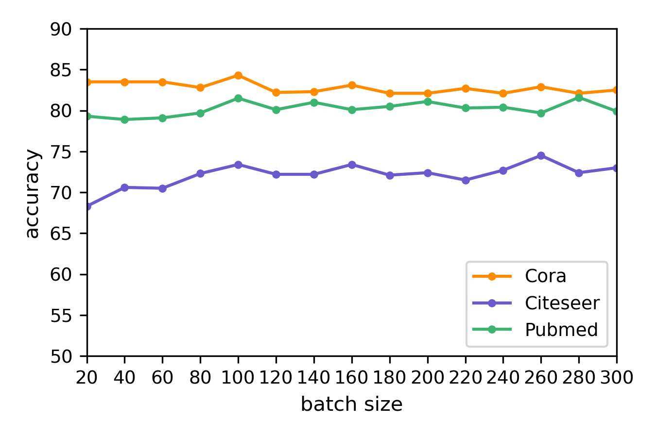
(a) Results on batch size

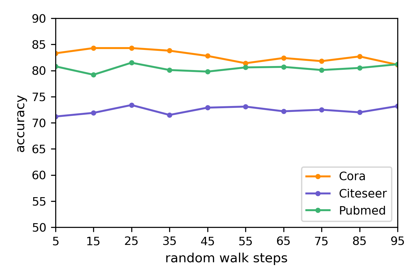
(b) Results on random walk length

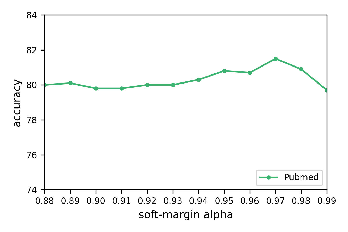
(c) Results on soft-margin $\alpha$

Figure 3: Parameter analysis results.

From this figure, we have following observations. First, we highlight that our model is insensitive to parameter “batch size” and “random walk length ”, as shown in Fig 3(a) and 3(b). Second, our model is obviously sensitive to the soft-margin parameter $\alpha$ which controls the ratio of of selecting potential positive samples from the negative samples set . It is also well noticed that when $\alpha$ is close to 1, the model performance dramatically drops. This verifies that negative samples sampling is crucial to the model performance of the contrastive learning.

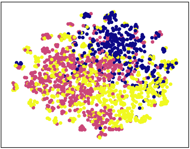
(a) Raw features

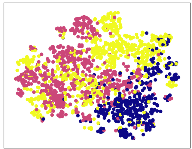
(b) Mvgrl

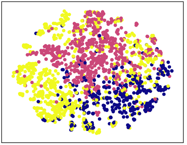
(c) Ours

Figure 4: Visualizing the learnt embeddings of nodes on Pubmed dataset. In this figure, each color represents one underlying true class, and each colored point represent the embeddings of a node.

5.5 RQ4: Visualization Results

Due to page limitations, we choose to visualize the node embeddings learnt on Pubmed dataset to provide a vivid illustration of the proposed model performance. As there are many nodes in Pubmed, we randomly selected 2000 nodes to plot. We also visualized the results of the Mvgrl method for comparison as this approach achieves the superior node classification results. The visualization results are plotted in Figure 4. Obviously, our model achieves the best visualization results on Pubmed dataset. It is noticed that in the raw features, most of the “red” and “yellow” class are mixed up together, which makes the classification task difficult. It is also noticed that the three classes could be well separated and spread over the whole data space by our model, whilst the “red” class and “yellow” class are still mixed up in Figure 4(b). We can infer that our approach could verifies that node-level contrastive learning can learn informative low-dimensional representations.

6 Conclusion

In this paper, we propose a novel node-wise contrastive learning approach to learn node embeddings for a supervised task. Particularly, we propose to resolve class collision issue by transiting the detected “in doubt” negative instances from the negative instance set to the positive instance set. Furthermore, a DPP-based sampling strategy is proposed to evenly sample negative instances for the contrastive learning. Extensive experiments are evaluated on three real-world datasets and the promising results demonstrate that the proposed approach is superior to both the baseline and the SOTA approaches.

References

- [1] Abu-El-Haija, S., Perozzi, B., Kapoor, A., Alipourfard, N., Lerman, K., Harutyunyan, H., Steeg, G.V., Galstyan, A.: MixHop: Higher-order graph convolutional architectures via sparsified neighborhood mixing. In: Proceedings of the 36th International Conference on Machine Learning. vol. 97, pp. 21–29 (2019)
- [2] Borgwardt, K.M., Kriegel, H.P.: Shortest-path kernels on graphs. In: Fifth IEEE International Conference on Data Mining (ICDM’05). pp. 8–pp (2005)
- [3] Chen, J., Ma, T., Xiao, C.: Fastgcn: Fast learning with graph convolutional networks via importance sampling. In: International Conference on Learning Representations (2018)
- [4] Defferrard, M., Bresson, X., Vandergheynst, P.: Convolutional neural networks on graphs with fast localized spectral filtering. In: Advances in Neural Information Processing Systems. vol. 29 (2016)
- [5] Giles, C.L., Bollacker, K.D., Lawrence, S.: Citeseer: An automatic citation indexing system. In: Proceedings of the Third ACM Conference on Digital Libraries, Pittsburgh, PA, USA. pp. 89–98 (1998)
- [6] Glorot, X., Bengio, Y.: Understanding the difficulty of training deep feed forward neural networks. In: Proceedings of the Thirteenth International Conference on Artificial Intelligence and Statistics. vol. 9, pp. 249–256. Chia Laguna Resort, Sardinia, Italy (2010)
- [7] Glorot, X., Bordes, A., Bengio, Y.: Deep sparse rectifier neural networks. In: Proceedings of the Fourteenth International Conference on Artificial Intelligence and Statistics. pp. 315–323. Fort Lauderdale, FL, USA (2011)
- [8] Grover, A., Leskovec, J.: node2vec: Scalable feature learning for networks. In: Proceedings of the 22nd ACM SIGKDD international conference on Knowledge discovery and data mining. pp. 855–864 (2016)
- [9] Hamilton, W.L., Ying, R., Leskovec, J.: Inductive representation learning on large graphs. In: Proceedings of the 31st International Conference on Neural Information Processing Systems. pp. 1025–1035 (2017)
- [10] Hassani, K., Khasahmadi, A.H.: Contrastive multi-view representation learning on graphs. In: International Conference on Machine Learning. pp. 4116–4126 (2020)
- [11] He, K., Fan, H., Wu, Y., Xie, S., Girshick, R.: Momentum contrast for unsupervised visual representation learning. In: Proceedings of the IEEE/CVF Conference on Computer Vision and Pattern Recognition. pp. 9729–9738 (2020)
- [12] Kalantidis, Y., Sariyildiz, M.B., Pion, N., Weinzaepfel, P., Larlus, D.: Hard negative mixing for contrastive learning. In: Advances in Neural Information Processing Systems. vol. 33, pp. 21798–21809 (2020)
- [13] Kingma, D.P., Ba, J.: Adam: A method for stochastic optimization. In: International Conference on Learning Representations, ICLR 2015, San Diego, CA, USA, May 7-9, 2015, Conference Track Proceedings (2015)
- [14] Kipf, T., Welling, M.: Semi-supervised classification with graph convolutional networks. In: International Conference of Learning Representations (2017)
- [15] Kipf, T.N., Welling, M.: Variational graph auto-encoders. arXiv preprint arXiv:1611.07308 (2016)
- [16] Liu, Z., Chen, C., Li, L., Zhou, J., Li, X., Song, L., Qi, Y.: Geniepath: Graph neural networks with adaptive receptive paths. In: Proceedings of the AAAI Conference on Artificial Intelligence. vol. 33, pp. 4424–4431 (2019)
- [17] Logeswaran, L., Lee, H.: An efficient framework for learning sentence representations. In: International Conference on Learning Representations (2018)
- [18] Macchi, O.: The coincidence approach to stochastic point processes. Advances in Applied Probability 7, 83–122 (1975)
- [19] Mccallum, A.K., Nigam, K., Rennie, J., Seymore, K.: Automating the construction of internet portals with machine learning. Information Retrieval 3(2), 127–163 (2000)
- [20] Namata, G., London, B., Getoor, L., Huang, B., EDU, U.: Query-driven active surveying for collective classification. In: 10th International Workshop on Mining and Learning with Graphs (2012)
- [21] Narayanan, A., Chandramohan, M., Chen, L., Liu, Y., Saminathan, S.: subgraph2vec: Learning distributed representations of rooted sub-graphs from large graphs (2016)
- [22] van den Oord, A., Li, Y., Vinyals, O.: Representation learning with contrastive predictive coding (2019)
- [23] Perozzi, B., Al-Rfou, R., Skiena, S.: Deepwalk: Online learning of social representations. In: Proceedings of the 20th ACM SIGKDD international conference on Knowledge discovery and data mining. pp. 701–710 (2014)
- [24] Qiu, J., Chen, Q., Dong, Y., Zhang, J., Yang, H., Ding, M., Wang, K., Tang, J.: Gcc. In: Proceedings of the 26th ACM SIGKDD International Conference on Knowledge Discovery & Data Mining (2020)
- [25] Ribeiro, L.F., Saverese, P.H., Figueiredo, D.R.: struc2vec: Learning node representations from structural identity. In: Proceedings of the 23rd ACM SIGKDD international conference on knowledge discovery and data mining. pp. 385–394 (2017)
- [26] Shervashidze, N., Vishwanathan, S., Petri, T., Mehlhorn, K., Borgwardt, K.: Efficient graphlet kernels for large graph comparison. In: Proceedings of the Twelth International Conference on Artificial Intelligence and Statistics. pp. 488–495 (2009)
- [27] Sun, F.Y., Hoffmann, J., Verma, V., Tang, J.: Infograph: Unsupervised and semi-supervised graph-level representation learning via mutual information maximization. In: International Conference on Learning Representations (2019)
- [28] Tang, J., Qu, M., Wang, M., Zhang, M., Yan, J., Mei, Q.: Line: Large-scale information network embedding. In: Proceedings of the 24th International Conference on World Wide Web. p. 1067–1077. International World Wide Web Conferences Steering Committee (2015)
- [29] Veličković, P., Cucurull, G., Casanova, A., Romero, A., Liò, P., Bengio, Y.: Graph attention networks. In: International Conference of Learning Representations (2018)
- [30] Veličković, P., Fedus, W., Hamilton, W.L., Liò, P., Bengio, Y., Hjelm, R.D.: Deep graph infomax. In: International Conference on Learning Representations (2019)
- [31] Xu, B., Shen, H., Cao, Q., Cen, K., Cheng, X.: Graph convolutional networks using heat kernel for semi-supervised learning. In: Proceedings of the Twenty-Eighth International Joint Conference on Artificial Intelligence (2019)
- [32] Xu, K., Li, C., Tian, Y., Sonobe, T., ichi Kawarabayashi, K., Jegelka, S.: Representation learning on graphs with jumping knowledge networks. In: International Conference on Machine Learning. pp. 5453–5462 (2018)
- [33] Yuan, H., Ji, S.: Structpool: Structured graph pooling via conditional random fields. In: International Conference on Learning Representations (2020)
- [34] Zhang, H., Cisse, M., Dauphin, Y.N., Lopez-Paz, D.: mixup: Beyond empirical risk minimization. In: International Conference on Learning Representations (2018)
- [35] Zhang, M., Chen, Y.: Link prediction based on graph neural networks. In: Proceedings of the 32nd International Conference on Neural Information Processing Systems. p. 5171–5181 (2018)
- [36] Zhu, X., Ghahramani, Z., Lafferty, J.: Semi-supervised learning using gaussian fields and harmonic functions. In: Proceedings of the 20th International conference on Machine learning (ICML-03). p. 912–919 (2003)
- [37] Zitnik, M., Leskovec, J.: Predicting multicellular function through multi-layer tissue networks. Bioinformatics 33, i190–i198 (2017)