Modeling the dominance of the gradient drift or Kelvin-Helmholtz instability in sheared ionospheric $\mathbf{E}\times\mathbf{B}$ flows

Abstract

Studies have shown that in sheared $\mathbf{E}\times\mathbf{B}$ flows in an inhomogeneous ionospheric plasma, the gradient drift (GDI) or the Kelvin-Helmholtz (KHI) instability may grow. This work examines the conditions that cause one of these instabilities to dominate over the other using a novel model to study localized ionospheric instabilities. The effect of collisions with neutral particles plays an important role in the instability development. It is found that the KHI is dominant in low collisionality regimes, the GDI is dominant in high collisionality regimes, and there exists an intermediate region in which both instabilities exist in tandem. For low collisionality cases in which the velocity shear is sufficiently far from the density gradient, the GDI is found to grow as a secondary instability extending from the KHI vortices. The inclusion of a neutral wind driven electric field in the direction of the velocity shear does not impact the dominance of either instability. Using data from empirical ionospheric models, two altitude limits are found. For altitudes above the higher limit, the KHI is dominant. For altitudes below the lower limit, the GDI is dominant. In the intermediate region, both instabilities grow together. Increasing the velocity shear causes both limits to be lower in altitude. This implies that for ionospheric phenomena whose density and velocity gradients span large altitude ranges, such as subauroral polarization streams, the instabilities observed by space-based and ground-based observation instruments could be significantly different.

I Introduction

The gradient drift instability (GDI), sometimes called the $\mathbf{E}\times\mathbf{B}$ or cross-field instability, is a plasma interchange instability that was initially studied in laboratory discharge experiments[1, 2]. A space charge or net current can develop in a perturbed, electrostatic, inhomogeneous, weakly ionized plasma in the presence of background electric and magnetic fields if there exists a difference in the effects of ion-neutral and electron-neutral collisions. This results in perturbed electric fields that drive perturbed $\mathbf{E}\times\mathbf{B}$ drifts causing instability growth. The GDI is a prominent structuring mechanism in the ionosphere[3, 4, 5] shown to cause ionospheric density irregularities in barium cloud experiments[6, 7, 8], polar cap patches[9, 10, 11], and diffuse aurora[12, 13, 14].

The Kelvin-Helmholtz instability (KHI) is a hydrodynamic instability that occurs at a velocity shear interface and induces the growth of vortical motion[15]. While the KHI exists ubiquitously in the universe, its primary role in the ionosphere is to generate high altitude turbulence[16]. The KHI can also occur as a secondary instability to the GDI[17, 18]. In large density gradient scale length regimes, the electrostatic KHI is damped by collisions[17].

The ionosphere can be categorized into three general regions (in order of increasing altitude): the D, E, and F regions. The maximum plasma density exists in the F region. Ionospheric plasma throughout all of the regions is a low-$\beta$ plasma ($\approx 10^{-6}$). The ionosphere coexists with the neutral thermosphere which depletes with altitude. Therefore, collision frequency with neutrals decreases with altitude. Thus, the effect of collisions is stronger in the D and E regions and weaker in the F region. This work focuses on the instability development in the F region where the collisions are weak enough to allow for both the GDI and KHI to grow.

Nonlocal linear theory on the GDI has shown that velocity shear acts to preferentially stabilize shorter wavelength modes[19, 20, 21]. Simulations have shown that velocity shear also prevents the extension of the GDI through regions of velocity shear[22]. However, in simulations with similar density and velocity profiles, the KHI has been shown to grow[17]. This paper examines which instability dominates under different parameter regimes.

The GDI and KHI are both important ionospheric structuring and turbulence generation mechanisms. Ionospheric turbulence can negatively impact radio communication signals. Therefore, understanding ionospheric turbulence can lead to predictive space weather forecasting and improved communication signals. Present simulation models, such as TIE-GCM[23], typically operate on global scales with resolutions of $0.625^{\circ}$. The novel model presented in this paper can examine instability development on scales of hundreds of meters.

Subauroral polarization streams (SAPS) are a specific ionospheric phenomenon in which turbulence has been observed. They are characterized by a latitudinally varying westward $\mathbf{E}\times\mathbf{B}$ driven flow[24] and are approximately co-located with a latitudinally varying density trough[25]. Additionally, many density and electric field irregularities have been observed in SAPS[26, 27, 28, 29, 30]. One of the primary mechanisms hypothesized to generate these is the GDI based on the density gradient morphology as well as observed turbulence spectra[27, 30], which has been corroborated by simulation[22]. However, alongside the density gradients are regions of velocity shear which may induce the KHI. Therefore, this work considers different collisional and spatial parameter regimes to determine which of the GDI or the KHI will dominate the instability development.

This paper is organized in the following manner. Section II provides a brief review of linear theory on the GDI and the KHI. It also makes predictions on the optimal GDI growth direction. Section III discusses the mathematical and computational models used in this work, as well as the model initialization. Section IV evaluates the predicted optimal GDI growth directions and examines several parameters that might determine which of the KHI or GDI are dominant. Section V interprets how the results apply to the ionosphere. Section VI provides a summary of the work. Appendix A discusses the derivation of the model in greater detail. Appendix B benchmarks the model to well known linear theory for the GDI and the KHI in slab geometries.

II Linear Theory

This section provides simplified linear growth rates used for direction and interpretation of the simulations. Comparisons of simulation results with established linear theory are provided in Appendix B.

II.1 GDI

The growth rate and maximum growth direction of the GDI are dependent on the strength of the collisions with neutrals. The effect of collisions is characterized by the dimensionless parameter $R$, which is

$$R=\frac{\nu_{in}}{\Omega_{ci}}-\frac{\nu_{en}}{\Omega_{ce}},$$ (1)

where $\nu$ is the collision frequency, $\Omega$ is the gyrofrequency, and the subscripts $i$, $e$, and $n$ denote the ions, electrons, and neutral particles respectively. In the E region, $R\gg 1$, which implies that the Hall current dominates[14]. In the F region, $0<R\ll 1$, which implies that the Pedersen current dominates[31]. When $R$ is exactly 0, the GDI is not expected to occur since no collisions are present.

An altitude independent analytical growth rate is presented in Eq. 16 from Ref. 32 for an arbitrary geometry. If the magnetic field is assumed to be purely in $\mathbf{\hat{z}}$ and the density gradient, wavenumber, and electric field are in the $xy$ plane, that equation simplifies to

$$\gamma_{GDI}=\Big{|}\frac{E}{BL_{N}^{g}}\Big{|}f,$$ (2)

where $E$ is the magnitude of the electric field, $B$ is the magnitude of the magnetic field, $L_{N}^{g}$ is the magnitude of the density gradient scale length defined as $L_{N}^{g}=n|\nabla n|^{-1}$, and $f$ is a geometric factor that is a function of the directions of the density gradient, electric field, magnetic field, and wavenumber. The electric field unit vector is defined to be $\mathbf{\hat{e}}=\cos\theta_{e}\mathbf{\hat{x}}+\sin\theta_{e}\mathbf{\hat{y}}$. The wavenumber unit vector is defined to be $\mathbf{\hat{k}}=\cos\theta_{k}\mathbf{\hat{x}}+\sin\theta_{k}\mathbf{\hat{y}}$. The density gradient unit vector is defined to be $\mathbf{\hat{g}}=\cos\theta_{g}\mathbf{\hat{x}}+\sin\theta_{g}\mathbf{\hat{y}}$. The angles $\theta_{e}$, $\theta_{g}$, and $\theta_{k}$ are in the $xy$ plane and defined to be positive counterclockwise of $\mathbf{\hat{x}}$. Based on these definitions, the geometric factor, $f$, is

$$f=\sin\big{(}\theta_{k}-\theta_{g}\big{)}\Big{[}\cos\big{(}\theta_{e}-\theta_{k}\big{)}-R\sin\big{(}\theta_{e}-\theta_{k}\big{)}\Big{]}.$$ (3)

If a random noise perturbation is assumed to seed the instability growth, then the primary structures that develop will be in the fastest growing direction. This direction can be found by maximizing Eq. 3 for $\theta_{k}$ resulting in

$$\theta_{k_{\max}}=\frac{1}{2}\Big{(}\theta_{e}+\theta_{g}-\tan^{-1}\frac{1}{R}\Big{)}+l\frac{\pi}{2}\qquad l=\pm 1,\pm 3,\pm 5\dots,$$ (4)

where $l$ is an integer denoting the periodicity of the maxima. Note that $l$ is required to be odd based on the second derivative test to obtain only the maxima. Similar representations of Eq. 4 are found in the literature [31, 32].

Eq. 2 is the GDI growth rate for a sufficiently collisional plasma. For a plasma in the inertial regime with a small $R$ such that $\nu_{in}\ll 4|E/BL_{N}^{g}|$, the GDI growth rate is[33]

$$\gamma_{GDI}=f\sqrt{\nu_{in}\frac{E}{BL_{N}^{g}}}.$$ (5)

Eq. 32 from Ref. 34 provides a generalized GDI growth rate with the inclusion of inertial terms under the assumption that $|\gamma|\ll\nu_{in}$. In this paper, the parameter $R$ is swept through different values such that each of these three GDI growth rate equations, (Eqs. 2 and 5 in this paper and Eq. 32 from Ref. 34) will be valid for different cases. There will also be cases such that none of these are valid due to the assumptions for the collisions. The optimal growth direction determined by Eq. 4 is independent of whether the GDI is in the collisional or inertial regime.

II.2 KHI

For a fluid with a density and velocity interface, the KHI growth rate is

$$\gamma_{KHI}=\frac{\rho_{1}\rho_{2}k(V_{1}-V_{2})}{(\rho_{1}+\rho_{2})^{2}},$$ (6)

where $\rho$ is the mass density, $V$ is the velocity, $k$ is the wavenumber, and the subscripts denote values on either side of the interface[15]. Eq. 6 applies to a sharp interface modeled by a Heaviside function. For a general hydrodynamic shear flow with a gradually transitioning interface, the growth rate decreases with a larger velocity gradient scale length or with a smaller density gradient scale length[35].

The effect of collisions with neutral particles plays an important role for the KHI in the electrostatic regime. Contrary to the hydrodynamic description of the KHI[35], decreasing the density gradient scale length can lead to a regime in which the KHI growth rate increases with higher collisionality[36]. The KHI in this regime is sometimes called the collisional shear instability. For a regime with large density gradient scale lengths, increased collisionality has a stabilizing effect on the KHI growth rate[17]. This latter regime is what is considered in this work primarily due to its applicability to subauroral polarization streams in the F region ionosphere.

Additionally, the magnetic field in this work is perpendicular to the velocity shear direction and therefore does not impact the instability growth[15].

III Model

III.1 Mathematical Model

A novel mathematical model focused on studying the temperature gradient instability[37] theoretically is presented by Ref. 38. The work presented here adapts the concepts from that model to develop a numerical framework to study the KHI and the GDI. Production and loss terms as well as the temperature source terms are not considered as they have a negligible impact on the development of the instabilities being modeled. This work, in contrast with Ref. 38, includes inertial terms to better understand the KHI, the inertial GDI, and the nonlinear turbulence cascade.

The F region plasma is modeled electrostatically as a 2D fluid. Only motion perpendicular to the magnetic field is considered. The continuity, momentum, and energy equations, respectively, for an arbitrary species $\alpha$, are

$$\frac{\partial n_{\alpha}}{\partial t}+\nabla\cdot(n_{\alpha}\mathbf{V}_{\alpha})=D\nabla^{2}n_{\alpha}$$ (7)

$$n_{\alpha}\Big{(}\frac{\partial}{\partial t}+\mathbf{V}_{\alpha}\cdot\nabla\Big{)}\mathbf{V}_{\alpha}=\frac{q_{\alpha}n_{\alpha}}{m_{\alpha}}(\mathbf{E}+\mathbf{V}_{\alpha}\times\mathbf{B})$$

$$-\frac{\nabla P_{\alpha}}{m_{\alpha}}-n_{\alpha}\nu_{\alpha n}(\mathbf{V}_{\alpha}-\mathbf{u})$$ (8)

$$\frac{3}{2}n_{\alpha}k_{B}\frac{\partial T_{\alpha}}{\partial t}+\frac{3}{2}n_{\alpha}k_{B}\mathbf{V}_{\alpha}\cdot\nabla T_{\alpha}+n_{\alpha}k_{B}T_{\alpha}\nabla\cdot\mathbf{V}_{\alpha}=0$$ (9)

where $D$ is an numerical diffusion constant, $\mathbf{u}$ is the neutral wind speed, and $\nu_{\alpha n}$ is the collision frequency between species $\alpha$ and neutral particles. The only species evolved in this model are ions and electrons; the effect of the neutral particles is considered in the collisional momentum source term. The equation of state is the ideal gas law. The collision frequencies are calculated using $\nu_{\alpha n}=n_{n}V_{Th_{\alpha}}\sigma_{\alpha n}$, where $n_{n}$ is the neutral number density, $V_{Th_{\alpha}}$ is the thermal velocity, and $\sigma_{\alpha n}$ is the collision cross-section. The energy equation, Eq. 9, is included in the model and is solved computationally, but has a negligible impact on these instabilities in this parameter regime. Therefore, the emphasis is placed on Eqs. 7 and 8.

The velocities are found from Eq. 8 and split into zeroth and first order in terms of the form $\nu_{\alpha n}/\Omega_{c\alpha}$ or $(\partial/\partial t+\mathbf{V}\cdot\nabla)/\Omega_{c\alpha}$, where $\Omega_{c\alpha}$ is the gyrofrequency. The resulting velocities are

$$\mathbf{V}_{e}^{0} =\frac{\mathbf{E}\times\mathbf{B}}{B^{2}}+\frac{\nabla P_{e}\times\mathbf{B}}{eB^{2}n_{e}}$$ (10)

$$\mathbf{V}_{e}^{1} =-\frac{\nu_{en}}{\Omega_{ce}}\frac{\nabla P_{e}}{en_{e}B}-\frac{\nu_{en}}{B\Omega_{ce}}\Big{(}\mathbf{E}+\mathbf{u}\times\mathbf{B}\Big{)}$$

$$\ -\frac{1}{B\Omega_{ce}}\Big{(}\frac{\partial}{\partial t}+\mathbf{V}_{\mathbf{E}\times\mathbf{B}}\cdot\nabla\Big{)}\mathbf{E}$$ (11)

$$\mathbf{V}_{i}^{0} =\frac{\mathbf{E}\times\mathbf{B}}{B^{2}}-\frac{\nabla P_{i}\times\mathbf{B}}{eB^{2}n_{i}}$$ (12)

$$\mathbf{V}_{i}^{1} =-\frac{\nu_{in}}{\Omega_{ci}}\frac{\nabla P_{i}}{en_{i}B}+\frac{\nu_{in}}{B\Omega_{ci}}\Big{(}\mathbf{E}+\mathbf{u}\times\mathbf{B}\Big{)}$$

$$\ +\frac{1}{B\Omega_{ci}}\Big{(}\frac{\partial}{\partial t}+\mathbf{V}_{\mathbf{E}\times\mathbf{B}}\cdot\nabla\Big{)}\mathbf{E},$$ (13)

where the zeroth order velocities are a combination of the $\mathbf{E}\times\mathbf{B}$ and diamagnetic drifts.

The zeroth order velocities are used in the continuity and energy equations. Because the plasma is electrostatic, the electric field is defined as $\mathbf{E}=-\nabla\phi$. Due to the constant magnetic field, the diamagnetic drift term does not impact the continuity equation and therefore only the $\mathbf{E}\times\mathbf{B}$ drift advects the plasma. The plasma is assumed to be quasineutral such that $n_{i}=n_{e}=n$, and thus, only one continuity equation is needed. Furthermore, the current is closed using $\nabla\cdot\mathbf{J}=0$ where $\mathbf{J}=ne(\mathbf{V}_{i}-\mathbf{V}_{e})$ where both the zeroth and first order velocities are used to calculate $\mathbf{J}$. Therefore, the relevant equations, continuity and current closure, are

$$\frac{\partial n}{\partial t}-\frac{\nabla\phi\times\mathbf{B}}{B^{2}}\cdot\nabla n=D\nabla^{2}n$$ (14)

$$\nabla\cdot\Big{(}n\nabla\frac{\partial\phi}{\partial t}\Big{)}=\Big{(}\frac{1}{\Omega_{ci}}+\frac{1}{\Omega_{ce}}\Big{)}^{-1}\bigg{[}-\frac{\nu_{in}}{e\Omega_{ci}}\nabla^{2}P_{i}+\frac{\nu_{en}}{e\Omega_{ce}}\nabla^{2}P_{e}\\ +\Big{(}\frac{\nu_{in}}{\Omega_{ci}}+\frac{\nu_{en}}{\Omega_{ce}}\Big{)}\Big{(}\mathbf{u}\times\mathbf{B}\cdot\nabla n-\nabla\cdot[n\nabla\phi]\Big{)}\bigg{]}\\ -\nabla\cdot\Big{(}n\mathbf{V}_{\mathbf{E}\times\mathbf{B}}\cdot\nabla\nabla\phi\Big{)}.$$ (15)

The $\mathbf{u}\times\mathbf{B}$ term can be considered an applied electric field, $\mathbf{E}_{0}$. This field is the result of a Lorentz transformation into the frame of reference of the neutral particles. Note that the numerical diffusion term in Eq. 14 provides isotropic diffusion to mitigate numerical error, preferentially acting on higher wavenumber modes.

Traditionally, fundamental physics simulations of plasma instabilities are required to start in an equilibrium state. This is done by initializing all but one of the variables and allowing the remaining variable to be solved for such that the system is in an equilibrium. However, the governing equations and collision frequencies are highly coupled. Assigning any one variable as the equilibrium variable would have significant consequences for the growth of the GDI or the KHI. Therefore, to maintain an equilibrium, a perturbed model is developed such that the background does not change and only the perturbation is evolved. This inherently makes the assumption that the time scales of turbulence evolution are much faster than the time scales of the background dynamics. This can also be seen as a method of accounting for other physics, such as motion parallel to the magnetic field, that exist in nature to maintain a quasi-equilibrium. The variables $\phi$, $n$, $T_{i}$, and $T_{e}$ are split into background and perturbed quantities, e.g., $\phi=\phi_{bg}+\phi_{p}$. When substituting these terms into Eqs. 14 and 15, terms containing only background quantities are removed. Thus, only terms with perturbed quantities remain. Based on the background geometry of the problem, as discussed in Section III.2, the continuity and energy residuals already satisfy the criterion of removing the background quantities. Thus, this method only needs to be applied to the continuity temporal derivative, the continuity source term, and the entire current closure equation. The resulting perturbed set of equations are

$$\frac{\partial n_{p}}{\partial t}-\frac{\nabla\phi\times\mathbf{B}}{B^{2}}\cdot\nabla n=D\nabla^{2}n_{p}$$ (16)

$$\nabla\cdot\Big{(}n\nabla\frac{\partial\phi_{p}}{\partial t}\Big{)}=\Big{(}\frac{1}{\Omega_{ci}}+\frac{1}{\Omega_{ce}}\Big{)}^{-1}\bigg{[}-\frac{\nu_{in}}{e\Omega_{ci}}\nabla^{2}P_{i_{p}}+\frac{\nu_{en}}{e\Omega_{ce}}\nabla^{2}P_{e_{p}}+\Big{(}\frac{\nu_{in}}{\Omega_{ci}}+\frac{\nu_{en}}{\Omega_{ce}}\Big{)}\Big{(}\mathbf{u}\times\mathbf{B}\cdot\nabla n_{p}-\nabla\cdot[n_{p}\nabla\phi+n_{bg}\nabla\phi_{p}]\Big{)}\bigg{]}\\ -\nabla\cdot\Big{(}n_{bg}\mathbf{V}_{\mathbf{E}\times\mathbf{B}_{bg}}\cdot\nabla\nabla\phi_{p}+n_{bg}\mathbf{V}_{\mathbf{E}\times\mathbf{B}_{p}}\cdot\nabla\nabla\phi+n_{p}\mathbf{V}_{\mathbf{E}\times\mathbf{B}}\cdot\nabla\nabla\phi\Big{)}.$$ (17)

The derivation of the model is discussed in greater detail in Appendix A.

Spatially, the equations are discretized using a pseudo-spectral method with a Fourier basis [39]. This converts the spatial derivatives into algebraic expressions, resulting in a set of temporal ordinary differential equations (ODEs). Periodic boundary conditions in all dimensions are required for the basis chosen for this discretization method. The temporal derivative term in Eq. 17, $\nabla\cdot(n\nabla\partial\phi_{p}/\partial t)$, cannot be isolated. An iterative method is used to calculate $\partial\phi_{p}/\partial t$. This results in a linear system of temporal ODEs that are integrated using a four stage fourth order Runge-Kutta method[40].

III.2 Background and Initial Conditions

For all of the simulations presented in this paper, the functional forms of the background variables are the same.

The background density is defined by a set of two hyperbolic tangent functions of the form

$$n_{bg}(x)=n_{0}\bigg{(}c+\sum_{i=1}^{2}a_{i}\tanh\Big{[}\frac{x-x_{N_{i}}}{L_{N}}\Big{]}\bigg{)},$$ (18)

where $n_{0}$ is a reference density, $L_{N}$ is a length scaling factor, $x_{N}$ defines the location of the density interfaces, and the constants $a$ and $c$ determine the levels of each region of the hyperbolic tangents. All of the simulations in Section IV use $n_{0}=10^{11}$ $\mathrm{m}^{-3}$, $a_{1}=-0.75$, $a_{2}=0.75$ and $c=1$. The parameters $L_{N}$ and $x_{N_{i}}$ vary.

Similarly, the background velocity is defined by four hyperbolic tangent functions of the form

$$V_{y_{bg}}(x)=\frac{V_{0}}{2}\sum_{i=1}^{4}b_{i}\tanh\Big{(}\frac{x-x_{V_{i}}}{L_{V}}\Big{)},$$ (19)

where $V_{0}$ is a reference velocity, $L_{V}$ is a length scaling factor, and $x_{V}$ is the location of the velocity interfaces. Because the background velocity is purely $\mathbf{E}\times\mathbf{B}$ driven, the two additional hyperbolic tangent functions are included to ensure periodicity in the electric potential, which is calculated using $\phi_{bg}(x)=B\int V_{y_{bg}}(x)dx$. The constants $b_{i}$ are defined to be $b_{1}=1$, $b_{2}=-1$, $b_{3}=-1$, and $b_{4}=1$. To maintain periodicity, $x_{V_{3,4}}$ are defined as $x_{V_{3}}=L_{x}-x_{V_{2}}$ and $x_{V_{4}}=L_{x}-x_{N_{1}}$, where $L_{x}$ is the domain length in $x$. All of the simulations use $L_{V}=10$ km and $x_{V_{2}}=700$ km. The parameters $V_{0}$ and $x_{V_{1}}$ vary.

The background ion and electron temperatures are constants with $T_{i_{bg}}=T_{e_{bg}}=1000$ K. The neutral species is atomic oxygen (O) and the ion species is singly ionized atomic oxygen (O⁺). The background magnetic field is $B=$5\text{\times}{10}^{-5}\text{\,}\mathrm{T}$$. The density is initialized with a random noise perturbation of $10^{-6}n_{0}$. The domain length, number of grid points, numerical diffusion constant, neutral number density, and neutral wind vary between simulations. All of the parameters have been chosen to reasonably align with observed values in subauroral polarization streams or the F region ionosphere in general. The chosen parameters show that the fluid approximation is valid with the Debye length ($4\text{\times}{10}^{-3}\text{\,}\mathrm{m}$), the ion ($3\text{\,}\mathrm{m}$) and electron ($1\text{\times}{10}^{-2}\text{\,}\mathrm{m}$) gyroradii, the skin depth ($10\text{\,}\mathrm{m}$), and ion inertial length ($1.8\text{\times}{10}^{3}\text{\,}\mathrm{m}$) not being adequately resolved by the smallest used grid size of $732\text{\,}\mathrm{m}$. Since the phenomena considered are at much larger scales, the inherent model assumptions cannot capture kinetic physics.

IV Results

IV.1 Optimal GDI Growth Direction as a Diagnostic

A set of simulations is run to test the validity of Eq. 4 in predicting the direction of GDI growth. This is a useful diagnostic for Sections IV.2 and IV.3 to verify that some of the instability structures that develop are the GDI based on the direction of growth. It is tested by changing the direction of the applied electric field. The electric field for each case is initialized such that the magnitude remains constant but the angle is varied from 0 to $7\pi/4$ in increments of $\pi/4$ for a total of 8 cases. Since the applied electric field is based on the neutral wind, the neutral wind is initialized as $\mathbf{u}=u\cos(\theta_{e}+\pi/2)\mathbf{\hat{x}}+u\sin(\theta_{e}+\pi/2)\mathbf{\hat{y}}$, where $u=500$ m/s. Since the initial density perturbation is random white noise, the dominant GDI that grows will have the highest growth rate, as per Eq. 2. This highest growth rate should occur for a wavenumber with an angle defined by Eq. 4.

The domain length is $L=500\times 250$ km with $256\times 512$ grid points. The parameters for the background density profile are $L_{N}=30$ km, $x_{N_{1}}=125$ km, and $x_{N_{2}}=375$ km. The background velocity profile is turned off by setting $V_{0}=0$ m/s. The numerical diffusion constant is $10^{3}$ $\mathrm{m}^{2}\mathrm{/}\mathrm{s}$. The neutral number density is $n_{n}=10^{14}$ $\mathrm{m}^{-3}$.

Figure 1 shows the results of this set of simulations. The times are shown non-dimensionally with $\tilde{t}=uf_{\max}t/L_{N}^{g}$, where $L_{N}^{g}$ is the minimum density gradient scale length and $f_{\max}$ is the larger geometric factor (from Eq. 3) between the left and right density interfaces. In all of the simulations, the GDI is shown to grow as “fingers” extending in both directions from the location of minimum density gradient scale length. The dashed cyan lines on each plot indicate the direction of predicted GDI growth. Note that the direction of the visual GDI growth, i.e., the “fingers”, is perpendicular to the GDI propagation direction. Therefore, the slopes of the dashed cyan lines represent the angles of $\theta_{k_{\max}}\pm\pi/2$. Because there are two density interfaces, the effect of changing $\theta_{g}$ is also considered. The left density interfaces have $\theta_{g}=\pi$ and the right density interfaces have $\theta_{g}=0$. Based on $\theta_{g}$ and $\theta_{e}$, the GDI visually extends in the directions predicted by the dashed cyan lines validating the linear theory prediction of Eq. 4 (note that further benchmarking of the GDI to linear theory is provided in Appendix B). The geometric factor, $f$, is different for each density interface because of the different directions of $\theta_{g}$. Because of this, one interface may have a larger growth rate than the other and therefore dominates the growth. This is seen in Figures 1(b-d) where the GDI grows on the right interface and in Figure 1(f-h) where the GDI grows on the left interface. Given a longer period of time, the GDI is expected to slowly grow at the opposite interface. However, Figures 1(c) and 1(g) show special cases in which the GDI does not grow on the opposite interface because $f=0$ at that interface.

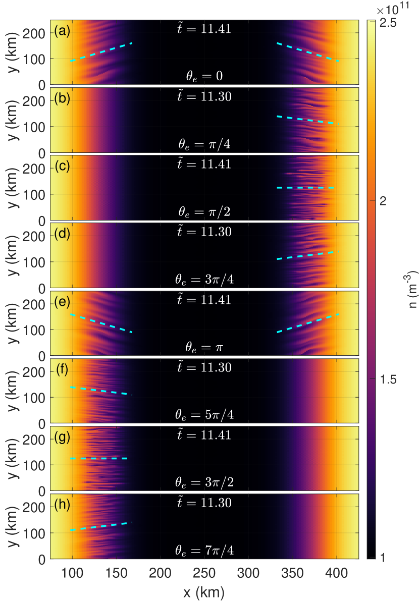
Figure 1: Density plots showing the development of the GDI for $\theta_{e}$ from 0 to $7\pi/4$. The dashed cyan lines indicate the direction of predicted visual growth based on the Eq. 4. Note that the visual growth of the GDI is perpendicular to the optimal wavenumber direction, $\theta_{k_{\max}}$. For all cases, the GDI extends in the predicted directions. Depending on the value of $\theta_{e}$, the growth at a particular interface, based on Eq. 3, may be significantly stronger than at the other interface. For this reason, the GDI only grows at the right density interface for Panels (b-d) and at the left density interface for Panels (f-h).

IV.2 Effect of Collisions

Section II.1 describes the importance of the parameter $R$ on the GDI growth through Eqs. 2 and 3. For large density gradient scale lengths, the KHI grows more quickly at low $R$[17]. The effect of varying $R$ has previously been studied on the independent development of the GDI[41] and the KHI[17], but not on the combined effect of these two instabilities.

Simulations are performed to sweep through different $R$ to understand the effect of collisions on instability development looking at the combination of the GDI and the KHI. Note that $R$ still needs to be sufficiently small such that the assumptions made in Section III.1 for an F region plasma are not violated. The parameter $R$ is changed by varying the neutral number density from $5\text{\times}{10}^{12}\text{\,}\mathrm{m}^{-3}$ to $3\text{\times}{10}^{13}\text{\,}\mathrm{m}^{-3}$ which corresponds to a range of $R$ from $4.62\text{\times}{10}^{-6}$ to $2.95\text{\times}{10}^{-5}$. These $R$ correspond to an altitude range of approximately 700 km down to 530 km (from Figure 7). These $R$ values are chosen to provide approximate limits as to when either the GDI or the KHI dominates over the other for this velocity profile. In this paper, the word dominate refers to when one instability visually grows much more quickly than the other.

The domain length is $1500\times 1000$ km with $1024\times 256$ grid points. The parameters for the background density profile are $L_{N}=50$ km, $x_{N_{1}}=220$ km, and $x_{N_{2}}=1200$ km. The parameters for the background velocity profiles are $V_{0}=-1000$ m/s and $x_{V_{1}}=220$ km. The numerical diffusion constant is $10^{4}$ $\mathrm{m}^{2}\mathrm{/}\mathrm{s}$. The velocity magnitude corresponds to observed values in subauroral polarization streams (SAPS)[28]. The neutral wind is set to 0 m/s.

Figure 2 shows the resulting density color plots of the instability development with increasing $R$ from left to right. The white curve represents the absolute value of the velocity profile such that there is a velocity of 0 m/s on the left of the velocity interface and a velocity of -1000 m/s on the right of the velocity interface. The times are shown non-dimensionally with $\tilde{t}=|tV_{0}/L_{N}^{g}|$. The top panels of Figure 2 show the early time development of the instabilities and the bottom panels show the late time nonlinear development of the instabilities.

Figures 2(a-b) show the classical vortical KHI structures at the velocity interface. The linear growth of Figure 2(a) reasonably matches established linear theory based on Figure 3 from Ref. 17. Further discussion of the benchmarking of the KHI is presented in Appendix B. Note that Figure 2(b) shows the KHI having a significantly smaller amplitude than that of Figure 2(a) because the KHI becomes more damped with increasing collision frequency in regimes of large density gradient scale lengths[17]. For these two cases, the KHI is the dominating instability early in time. Figure 2(c) shows the “finger-like” structures of the GDI growing in the direction predicted by Eq. 4, which is shown by the blue line. At early time, only the case with the highest collisionality shows any growth of the GDI.

Figure 2(d) shows that the lowest collisionality case develops into a set of nonlinear KHI vortices with cascading turbulence but no indication of any GDI development. Figures 2(e), however, shows that the GDI begins to develop at late times. Figure 2(f) shows the nonlinear evolution of the GDI. At late times, the GDI structures curve because the entire instability region is moving in the negative $\mathbf{\hat{y}}$ direction. An additional feature that develops is a secondary KHI, as shown by the curving “mushroom-like” structures. For larger $R$, the secondary KHI are expected to become increasingly damped[41]. Therefore, for low $R$, the KHI dominates, and for high $R$, the GDI dominates. In the intermediate region, both instabilities grow in tandem.

Figure 2: Density color plots showing instability development for different $R$ increasing to the right. Panels (a-c) display the early time growth whereas Panels (d-f) show the late time nonlinear development. The white curve represents the absolute value of the background velocity profile with $V_{0}=-10^{3}$ m/s. The transition from a pure KHI to a pure GDI is shown as $R$ increases. Note how the vortical structures gradually disappear and how the “finger-like” structures gradually increase as $R$ increases. In Panel (c), the blue line indicates the expected direction of GDI growth based on Eq. 4.

Figure 2 shows that the collisional parameter $R$ plays an important role in determining which instability dominates the growth. A parameter that can enhance the growth of both instabilities is the velocity magnitude, $V_{0}$. A set of simulations is run with varying $R$ by varying the neutral density from $7\text{\times}{10}^{12}\text{\,}\mathrm{m}^{-3}$ to $6\text{\times}{10}^{13}\text{\,}\mathrm{m}^{-3}$, which corresponds to a range of $R$ from $6.89\text{\times}{10}^{-6}$ to $5.90\text{\times}{10}^{-5}$. These $R$ correspond to an altitude range of approximately 670 km down to 490 km (from Figure 7). In these simulations, the background velocity is set to $V_{0}=-2000$ m/s. Velocities this high can occur in subauroral ion drifts (SAID), which are latitudinally narrower than SAPS[42]. The remaining parameters are the same as those used in Figure 2 except for the numerical diffusion constant which is set to $4\text{\times}{10}^{4}\text{\,}\mathrm{m}^{2}\mathrm{/}\mathrm{s}$.

Figure 3 shows the resulting instability development with $R$ increasing to the right. The time is presented non-dimensionally with $\tilde{t}=|tV_{0}/L_{N}^{g}|$. The top panels are early in time and the bottom panels are late in time. Qualitatively, the results are consistent with the transition from the KHI to GDI with increasing $R$ from Figure 2. The impact of a higher background velocity increases the region of KHI dominance. Because of this, the transition between the KHI and the GDI occurs at higher $R$. Once $R$ is sufficiently high, the GDI dominates and shows the same general structure as in Figure 2(c).

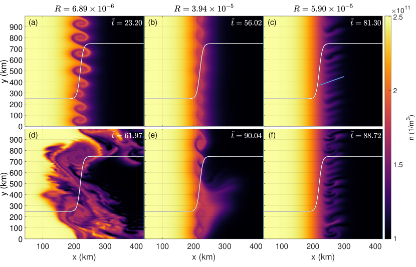
Figure 3: Density color plots showing instability development for different $R$ increasing to the right. Panels (a-c) show the early time development and Panels (d-f) show the late time development. The white curve represents the background velocity profile with $V_{0}=-2000$ m/s. The qualitative behavior of the transition from the KHI to the GDI matches that of Figure 2. Due to the higher background velocity, the transition from the KHI to the GDI occurs at a higher $R$. Thus, the KHI is more sensitive to increases in the velocity than the GDI is. Panel (c) shows the GDI dominating with the blue line representing the expected growth direction, which is the same as that of Figure 2(c).

IV.3 Effect of Velocity Shear Location

It is clear that the dominant instability transitions from the KHI to the GDI with increasing collisionality or decreasing velocity shear. It is possible that the background velocity profile chosen for Figure 2 may not be ideally conducive to GDI growth. Velocity shear has a stabilizing effect on the GDI that preferentially impacts shorter wavelength modes [19, 20, 21]. The region of velocity shear overlaps the region of the density gradient. In SAPS however, the location of the velocity shear does not necessarily have to be co-located with the density gradient[22]. If the region of velocity shear is sufficiently far from the density gradient, then the GDI may become more prominent even in the low collisionality regime. Note that the region of constant velocity must overlap the density gradient to induce the GDI. Therefore, in this case, the velocity shear location needs to be moved to the left, i.e., $x_{V_{1}}$ needs to be smaller.

A set of simulations is run examining different locations of the velocity shear. Two cases are run with the parameter $x_{V_{1}}$ set to 200 km and 150 km. The remaining parameters are the same as those in Figure 2(a) except with a resolution of $2048\times 512$ grid points.

Figure 4 shows the results of these simulations in the late time nonlinear phase of instability growth. The time is presented non-dimensionally as $\tilde{t}=|tV_{0}/L_{N}^{g}|$. At early times, Figure 4 looks similar to the KHI growth in Figure 2(a). Figure 4(a) shows a case where the velocity profile is shifted slightly to the left, where the KHI is still the dominant instability. Note that the small structures extending to the bottom right from the KHI vortices are the result of a turbulence cascade. In Figure 4(b), the velocity shear is sufficiently far from the density gradient to induce some sort of GDI growth. KHI vortices can be seen at the location of velocity shear. Extending from the right of these vortices are two long wavelength structures. Because the KHI vortex is generally circular, the value of $\theta_{g}$ can vary from $\pi/2$ to $\pi$. The blue lines indicate the directions of predicted GDI growth; the top line is uses $\theta_{g}=3\pi/4$ and the bottom line uses $\theta_{g}=\pi$. Note that $\theta_{e}=0$ for both lines. Very quickly afterwards, the GDI enters the nonlinear regime and becomes difficult to differentiate from the KHI. Therefore, the GDI appears to grow in situations where the velocity shear location is sufficiently far from the density gradient even in low collisionality regimes.

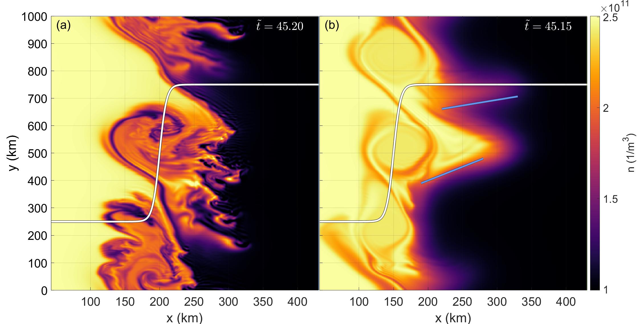
Figure 4: Density color plots showing KHI development for different velocity shear locations ($x_{V_{1}}$). The white curve represents the velocity profile. Panel (a) shows that the KHI is the dominant instability. Panel (b) has a velocity profile sufficiently far away from the density gradient. In addition to the KHI that grows at the velocity shear interface, there is a long wavelength growth on the right that occurs in the direction of expected GDI growth (light blue line).

Based on Eq. 2, adding an applied homogeneous electric field through the neutral wind can increase the growth rate of the GDI. Based on the geometry of Figure 4, the electric field direction that would maximize the growth rate is in the $-\mathbf{\hat{y}}$ direction, which corresponds to a neutral wind in the $\mathbf{\hat{x}}$ direction. A set of simulations are run with the same parameters as those in Figure 4 but with an $\mathbf{\hat{x}}$ direction neutral wind of 500 m/s. This magnitude is chosen because it represents the upper range of what would exist in the ionosphere [43].

Figure 5 shows the late stage instability development with the neutral wind. The time is presented non-dimensionally as $\tilde{t}=|tV_{0}/L_{N}^{g}|$. The neutral wind has an enhancing effect on the KHI which is seen by the significantly larger amplitude for both cases as compared to Figure 4 despite being at similar times. However, the neutral wind does not impact the transition of the KHI to the GDI with Figure 5(a), similar to Figure 4(a), being dominated by the KHI. Figure 5(b) shows much clearer “finger-like” structures suggesting the growth of the GDI. Similar to Figure 4(b), the density gradient direction can vary from $\pi/2$ to $\pi$ due to the generally circular nature of the KHI vortex which leads to different optimal GDI growth directions. Three blue lines indicate the different GDI growh directions. Starting from the top line, the density gradient directions used are $\theta_{g}=3\pi/4$, $\pi/2$, and $\pi$. Note that in this case, because of the addition of the neutral wind, $\theta_{e}=-0.4636$.

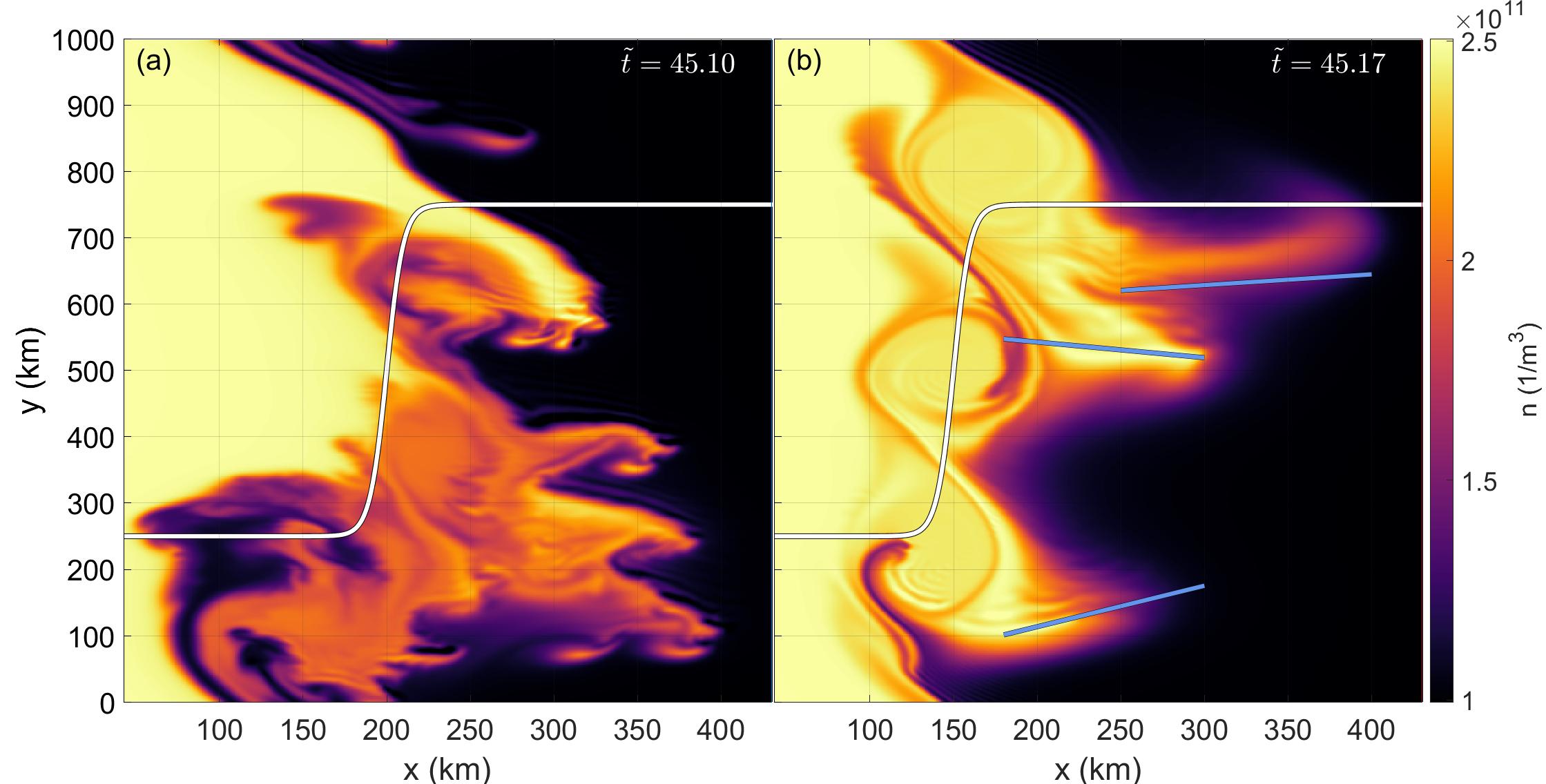
Figure 5: Density color plots showing KHI development using the same parameters as Figure 4 but with an $\mathbf{\hat{x}}$ direction neutral wind of 500 m/s. The neutral wind has an enhancing effect on the KHI growth in both cases. The KHI is the dominant instability in Panel (a). Panel (b) shows the GDI growing on the right side of the KHI. Light blue lines show the expected growth directions for different density gradient directions for the secondary GDI.

To show that the GDI is secondary to the KHI in the cases of Figures 4(b) and 5(b), a set of simulations are run using those same parameters but with $V_{0}=0$ m/s, $u_{y}=1000$ m/s, and a resolution of $1024\times 256$ grid points. This neutral wind drives the equivalent electric field that causes the background $\mathbf{E}\times\mathbf{B}$ drift but is constant throughout the entire domain. Figure 6 shows results with the time normalized as $\tilde{t}=|tu_{y}/L_{N}^{g}|$, which in this case is equivalent to the time normalizations in Figures 4(b) and 5(b). The GDI grows in this low collisionality regime but at a much slower rate compared to Figures 4(b) and 5(b). Therefore, the GDI in Figures 4(b) and 5(b) is a secondary instability that is seeded by the primary KHI.

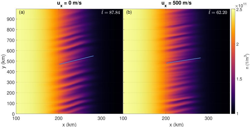
Figure 6: Panels (a) and (b) show the density color plots using the equivalent homogeneous applied electric field to Figures 4(b) and 5(b), respectively. The blue line indicates the direction of optimal GDI growth. The growth of the GDI takes significantly longer than the growth of the GDI shown in Figures 4(b) and 5(b).

V Discussion

Previous works have described formulae for the optimal GDI growth rate directions[31, 32]. Eq. 4 provides a generalized form as a function of $R$, $\theta_{g}$, and $\theta_{e}$. Ref. 17 examines this problem from a qualitative perspective noting that GDI growth is tilted in the generally expected direction for an angled electric field. Figure 1 provides a more comprehensive and detailed analysis showing that Eq. 4 accurately predicts the optimal direction of GDI growth. This provides a useful diagnostic tool for both simulation and observation. In simulations, the direction of any GDI growth can be predicted prior to running the simulation. For observation, the direction of observed GDI growth can provide information about possible unknowns such as the electric field direction, density gradient direction, or collisionality.

Several parameters have been examined to understand in which cases the GDI or KHI might grow. Figure 5 shows that the neutral wind has no impact on the transition between the GDI and the KHI. Figures 4 and 5 show that for certain velocity profiles at low $R$, the GDI develops as a secondary instability, based on Figure 6, in the nonlinear phase of the KHI. Linear theory and growth rates for this type of transition and secondary growth are highly nontrivial. Furthermore, the dominating instability in these cases is still the KHI. Figure 3 shows that the background velocity magnitude plays only a minor role despite the velocity being the approximate upper limit of what occurs in the ionosphere. Therefore, the collisional parameter $R$ is the main factor in determining which instability dominates, as shown in Figures 2 and 3. From a physical perspective, changing $R$ can also be thought of as changing the altitude because the neutral density is a strong function of altitude. Data from the IRI [44], NRLMSISE-00 [45], and IGRF [46] empirical ionospheric models are used to calculate $R$ as a function altitude. The input parameters used are for the date of May 2, 2013 at 20:00 local time at a geographic latitude and longitude of $57.5^{\circ}$ and $40^{\circ}$ respectively. Since the composition of the ionosphere and the thermosphere are also functions of altitude, a weighted average is used based on each species’ density to obtain effective masses and collision cross-sections. The ion and neutral particle collision cross-sections are obtained assuming hard sphere collisions using the appropriate species’ Van der Waals radius[47, 48]. The electron radius is assumed to be much smaller than the ion and neutral particle radii and is therefore set to 0 m.

Figure 7 shows the results of the example calculation of $R$ (blue line). Because of the effect of the neutral density, $R$ is found to decrease with increased altitude. Vertical red and orange dashed lines are plotted separating different regions of instablity behavior based on the background density and velocity profiles considered. For altitudes above the red dashed line, the KHI dominates, i.e., would grow first; for altitudes below the orange dashed line, the GDI dominates. In the intermediate region, both instabilities grow in tandem. Note that the blue curve is the same for Figures 7(a-b); the purpose of the two plots is to show how the altitude limits of the transition from the GDI to KHI change with differing background velocity shear. Figure 7(a) determines the different regions of dominance based on the results shown in Figures 2(a) and 2(c). Figure 7(b) determines the different regions of dominance based on the results shown in Figures 3(a) and 3(c). Figure 7(b) shows that increased velocity shear causes the transition region to occur at a lower altitude. The effect of decreasing plasma density with altitude is not expected to impact these results as both the GDI[32] and the KHI[15, 17] are impacted only by the density gradient scale length or density ratio and not the magnitude.

Note that Figure 7 is just an example calculation using simulation parameters from Figures 2 and 3. Additionally, the empirical parameters are found for a specific geographic location and time. Thus, Figure 7 does not apply to every case in the ionosphere. The key point is that there exists a region in altitude where the dominant instability will transition from the GDI to the KHI in certain sheared $\mathbf{E}\times\mathbf{B}$ flows. Subauroral polarization streams (SAPS) [24] have been observed to exhibit density irregularities[26, 27, 28, 29, 30]. Two instruments that have observed these are the Super Dual Auroral Radar Network (SuperDARN)[29] and DMSP satellites [27, 30]. SuperDARN radars operate at altitudes of approximately 300 km[49] whereas DMSP satellites have orbits of about 800 km[30]. Based on Figure 7 and with the correct SAPS velocity profiles, the DMSP satellites would observe the KHI as the dominant instability while the SuperDARN radars would observe the GDI as the dominant instability. Figure 7(b) shows that even for the upper limit of ionospheric velocity magnitudes, the DMSP satellites and SuperDARN radars would still only capture the KHI and GDI, respectively.

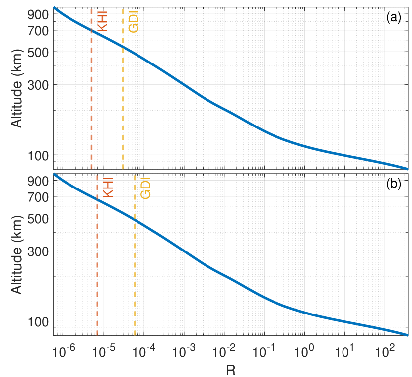
Figure 7: An example calculation of $R$ as a function of altitude using data from the IRI [44], NRLMSISE-00 [45], and IGRF [46] models. As altitude increases, $R$ decreases. The red and orange dashed lines represent the $R$ the altitude limits for the KHI and GDI respectively. Panel (a) sets the limits based on the results from Figure 2 and Panel (b) sets the limits based on the results from Figure 3. Above the red dashed line, the KHI will dominate; below the orange dashed line, the GDI will dominate. In the middle, both instabilities co-exist in some combination.

VI Summary and Conclusions

This paper has studied the gradient drift (GDI) and Kelvin-Helmholtz (KHI) instabilities using a model that solves a perturbed set of governing equations to understand parameter regimes in which each instability might dominate in a sheared $\mathbf{E}\times\mathbf{B}$ flow.

An analysis of the GDI linear theory provides a prediction on the fastest growing wavenumber direction. Simulations that vary the geometric conditions of the electric field and density gradient demonstrate the predictive capability providing a useful diagnostic tool for simulation and observation.

For the density and velocity profiles considered in this work, when modifying the collisional parameter, $R$, it is found that the KHI is the dominating instability at $R$ lower than $4.62\text{\times}{10}^{-6}$ and the GDI is the dominating instability at $R$ greater than $2.95\text{\times}{10}^{-5}$. For intermediate $R$ values, both instabilities exist in tandem. It is also found that the KHI is more sensitive to changes in the background velocity. For higher velocity cases, it is found that the KHI dominates for $R$ lower than $6.89\text{\times}{10}^{-6}$ and the GDI dominates for $R$ larger than $5.90\text{\times}{10}^{-5}$. This suggests that for higher velocities, the entire transition region occurs at a lower $R$ or, from a physical perspective, a lower altitude.

Velocity shear has a stabilizing effect on the GDI[19, 20, 21]. For a background velocity profile sufficiently far from the density gradient, a secondary GDI is formed that extends out of the KHI vortices. The inclusion of an applied electric field serves to increase the KHI amplitude as opposed to causing the GDI to dominate.

Since the collisionality is the primary factor in determining whether the KHI or the GDI are dominant, an example calculation of $R$ as a function of altitude is provided. Data are obtained from the IRI [44], NRLMSISE-00 [45], and IGRF [46] models. It is found that above a certain altitude, the KHI is the dominating instablity. Below another altitude, the GDI is the dominating instability. The implications are that with certain background density and velocity profiles that exist over large altitude ranges, the dominating instabilities observed by satellite versus ground based systems about the same phenomenon (in this case subauroral polarization streams) may be significantly different.

Data Availability Statement

The data that support the findings of this study are available from the corresponding author upon reasonable request.

Appendix A Model Derivation

This section presents the derivation of the model, which is adapted from a theoretical framework presented in Ref. 38. In addition, inertial terms are included to better study the KHI. The primary novelty is the development of the perturbed model to be able to study turbulence development in a wide array of physically relevant background profiles.

The continuity, momentum, and energy equations (Eqs. 7-9), rewritten here for convenience, are

$$\frac{\partial n_{\alpha}}{\partial t}+\nabla\cdot(n_{\alpha}\mathbf{V}_{\alpha})=D\nabla^{2}n_{\alpha}$$ (20)

$$n_{\alpha}\Big{(}\frac{\partial}{\partial t}+\mathbf{V}_{\alpha}\cdot\nabla\Big{)}\mathbf{V}_{\alpha}=\frac{q_{\alpha}n_{\alpha}}{m_{\alpha}}(\mathbf{E}+\mathbf{V}_{\alpha}\times\mathbf{B})$$

$$-\frac{\nabla P_{\alpha}}{m_{\alpha}}-n_{\alpha}\nu_{\alpha n}(\mathbf{V}_{\alpha}-\mathbf{u})$$ (21)

$$\frac{3}{2}n_{\alpha}k_{B}\frac{\partial T_{\alpha}}{\partial t}+\frac{3}{2}n_{\alpha}k_{B}\mathbf{V}_{\alpha}\cdot\nabla T_{\alpha}+n_{\alpha}k_{B}T_{\alpha}\nabla\cdot\mathbf{V}_{\alpha}=0.$$ (22)

The momentum equations, Eq. 21, can be solved for the velocity, $\mathbf{V}_{\alpha}$, in ordered terms of $\nu_{\alpha n}/\Omega_{c\alpha}$ and $(\partial/\partial t+\mathbf{V}\cdot\nabla)/\Omega_{c\alpha}$. In the F region ionosphere, these terms are considered small and thus only the zeroth and first order velocities are retained.

The model considers 2D motion perpendicular to the magnetic field. Taking the cross product of the electron momentum equation, Eq. 21 with $q_{e}=-e$, and the magnetic field and solving for $\mathbf{V}_{e}$ yields

$$\mathbf{V}_{e}=\mathbf{V}_{e}^{0}+\mathbf{V}_{e}^{1}+H.O.T.=\underbrace{\frac{\mathbf{E}\times\mathbf{B}}{B^{2}}+\frac{\nabla P_{e}\times\mathbf{B}}{en_{e}B^{2}}}_{\mathbf{V}_{e}^{0}}\\ +\frac{1}{B}\frac{\nu_{en}}{\Omega_{ce}}\Big{(}\mathbf{V}_{e}-\mathbf{u}\Big{)}\times\mathbf{B}+\frac{1}{B}\frac{1}{\Omega_{ce}}\Big{(}\frac{\partial}{\partial t}+\mathbf{V}_{e}\cdot\nabla\Big{)}\mathbf{V}_{e}\times\mathbf{B},$$ (23)

where $H.O.T.$ stands for higher order terms. The zeroth order electron velocity, denoted as $\mathbf{V}_{e}^{0}$ by the underbrace in Eq. 23, is a summation of the $\mathbf{E}\times\mathbf{B}$ and diamagnetic drifts. The remaining terms are of first order or higher.

The zeroth order ion velocity is needed to calculate the first order electron velocity. Similar to how Eq. 23 is obtained, the ion velocity is

$$\mathbf{V}=\mathbf{V}_{i}^{0}+\mathbf{V}_{i}^{1}+H.O.T.=\underbrace{\frac{\mathbf{E}\times\mathbf{B}}{B^{2}}-\frac{\nabla P_{i}\times\mathbf{B}}{en_{i}B^{2}}}_{\mathbf{V}_{i}^{0}}\\ -\frac{1}{B}\frac{\nu_{in}}{\Omega_{ci}}\Big{(}\mathbf{V}_{i}-\mathbf{u}\Big{)}\times\mathbf{B}-\frac{1}{B}\frac{1}{\Omega_{ci}}\Big{(}\frac{\partial}{\partial t}+\mathbf{V}_{i}\cdot\nabla\Big{)}\mathbf{V}_{i}\times\mathbf{B}.$$ (24)

The electron and ion velocities that appear on the right hand sides of Eqs. 23 and 24 can also be decomposed into zeroth, first, and higher order terms, which are all multiplied by terms of the form $\nu_{\alpha n}/\Omega_{c\alpha}$ or $(\partial/\partial t+\mathbf{V}\cdot\nabla)/\Omega_{c\alpha})$. Therefore, only the zeroth order terms remain as the first order terms become higher order terms. Thus, the first order electron and ion velocities are

$$\mathbf{V}_{e}^{1}=\frac{\nu_{en}}{B\Omega_{ce}}\Big{(}\frac{\mathbf{E}\times\mathbf{B}}{B^{2}}+\frac{\nabla P_{e}\times\mathbf{B}}{en_{e}B^{2}}-\mathbf{u}\Big{)}\times\mathbf{B}+\frac{1}{B\Omega_{ce}}\Big{(}\frac{\partial}{\partial t}+\Big{[}\frac{\mathbf{E}\times\mathbf{B}}{B^{2}}+\cancel{\frac{\nabla P_{e}\times\mathbf{B}}{en_{e}B^{2}}}\Big{]}\cdot\nabla\Big{)}\Big{(}\frac{\mathbf{E}\times\mathbf{B}}{B^{2}}+\cancel{\frac{\nabla P_{e}\times\mathbf{B}}{en_{e}B^{2}}}\Big{)}\times\mathbf{B}$$ (25)

$$\mathbf{V}_{i}^{1}=-\frac{\nu_{in}}{B\Omega_{ci}}\Big{(}\frac{\mathbf{E}\times\mathbf{B}}{B^{2}}-\frac{\nabla P_{i}\times\mathbf{B}}{en_{i}B^{2}}-\mathbf{u}\Big{)}\times\mathbf{B}-\frac{1}{B\Omega_{ci}}\Big{(}\frac{\partial}{\partial t}+\big{[}\frac{\mathbf{E}\times\mathbf{B}}{B^{2}}-\cancel{\frac{\nabla P_{i}\times\mathbf{B}}{en_{i}B^{2}}}\big{]}\cdot\nabla\Big{)}\Big{(}\frac{\mathbf{E}\times\mathbf{B}}{B^{2}}-\cancel{\frac{\nabla P_{i}\times\mathbf{B}}{en_{i}B^{2}}}\Big{)}\times\mathbf{B}.$$ (26)

For the F region phenomena considered in this work, the diamagnetic drift term is much smaller than the $\mathbf{E}\times\mathbf{B}$ drift terms. Thus, the diamagnetic terms are not considered in the convective derivative. After simplification, the zeroth order velocities are

$$\mathbf{V}_{e}^{0} =\frac{\mathbf{E}\times\mathbf{B}}{B^{2}}+\frac{\nabla P_{e}\times\mathbf{B}}{eB^{2}n_{e}}$$ (27)

$$\mathbf{V}_{i}^{0} =\frac{\mathbf{E}\times\mathbf{B}}{B^{2}}-\frac{\nabla P_{i}\times\mathbf{B}}{eB^{2}n_{i}},$$ (28)

and the first order velocities are

$$\mathbf{V}_{e}^{1} =-\frac{\nu_{en}}{\Omega_{ce}}\frac{\nabla P_{e}}{en_{e}B}-\frac{\nu_{en}}{B\Omega_{ce}}\Big{(}\mathbf{E}+\mathbf{u}\times\mathbf{B}\Big{)}$$

$$\ -\frac{1}{B\Omega_{ce}}\Big{(}\frac{\partial}{\partial t}+\mathbf{V}_{\mathbf{E}\times\mathbf{B}}\cdot\nabla\Big{)}\mathbf{E}$$ (29)

$$\mathbf{V}_{i}^{1} =-\frac{\nu_{in}}{\Omega_{ci}}\frac{\nabla P_{i}}{en_{i}B}+\frac{\nu_{in}}{B\Omega_{ci}}\Big{(}\mathbf{E}+\mathbf{u}\times\mathbf{B}\Big{)}$$

$$\ +\frac{1}{B\Omega_{ci}}\Big{(}\frac{\partial}{\partial t}+\mathbf{V}_{\mathbf{E}\times\mathbf{B}}\cdot\nabla\Big{)}\mathbf{E}.$$ (30)

Note that the inertia is primarily driven by the ions.

The zeroth order velocities, Eqs. 27 and 28, are used in the continuity and energy equations. The diamagnetic drift term does not play a role in the continuity equation due to the spatially constant magnetic field; thus, only the $\mathbf{E}\times\mathbf{B}$ drift advects the plasma. Furthermore, because the $\mathbf{E}\times\mathbf{B}$ drift is incompressible, the continuity equation can be written as

$$\frac{\partial n}{\partial t}-\frac{\nabla\phi\times\mathbf{B}}{B^{2}}\cdot\nabla n=D\nabla^{2}n,$$ (31)

where the electric field is $\mathbf{E}=-\nabla\phi$ where $\phi$ is the electric potential.

Assuming quasineutrality ($n_{i}=n_{e}=n$), the current closure equation is

$$\nabla\cdot\mathbf{J}=\nabla\cdot\Big{[}ne\big{(}\mathbf{V}_{i}-\mathbf{V}_{e}\big{)}\Big{]}=0,$$ (32)

where $\mathbf{J}$ is the current density. Subsituting Eqs. 27 to 30 into Eq. 32 and solving for the temporal derivative term yields

$$\nabla\cdot\Big{(}n\nabla\frac{\partial\phi}{\partial t}\Big{)}=\Big{(}\frac{1}{\Omega_{ci}}+\frac{1}{\Omega_{ce}}\Big{)}^{-1}\bigg{[}-\frac{\nu_{in}}{e\Omega_{ci}}\nabla^{2}P_{i}+\frac{\nu_{en}}{e\Omega_{ce}}\nabla^{2}P_{e}\\ +\Big{(}\frac{\nu_{in}}{\Omega_{ci}}+\frac{\nu_{en}}{\Omega_{ce}}\Big{)}\Big{(}\mathbf{u}\times\mathbf{B}\cdot\nabla n-\nabla\cdot[n\nabla\phi]\Big{)}\bigg{]}\\ -\nabla\cdot\Big{(}n\mathbf{V}_{\mathbf{E}\times\mathbf{B}}\cdot\nabla\nabla\phi\Big{)}.$$ (33)

For the problems considered in this paper, the energy equations play a negligible role in the instability development. While they are still solved, the emphasis is placed on Eqs. 31 and 33.

For problems in which the background dynamics are significantly slower than turbulence development, a perturbed model can be developed that maintains a background that is constant in time and only evolves perturbations. Each of the variables, $\phi$, $n$, $T_{i}$, and $T_{e}$, are split into background and perturbed quantities, e.g., $\phi=\phi_{bg}+\phi_{p}$. These terms are substituted into Eqs. 31 and 33. The equations are then expanded using the distributive property. Any terms that contain only background quantities are removed, and thus, only the perturbed terms remain.

For the continuity equation, Eq. 31, only the temporal derivative and the numerical diffusion source term need to be split in this way. The residual term automatically satisfies this condition because all of the background profiles used in Section IV are only functions of $x$ and the magnetic field is in the $\mathbf{\hat{z}}$ direction. Thus, the term $(\nabla\phi_{bg}\times\mathbf{B})\cdot\nabla n_{bg}$ is implicitly set to 0. As a simple example, the diffusion term is split into background and perturbed components as

$$D\nabla^{2}n=D\Big{(}\cancel{\nabla^{2}n_{bg}}-\nabla^{2}n_{p}\Big{)}=D\nabla^{2}n_{p}.$$ (34)

Because the diffusion term is linear, the final perturbed result looks the same as the original term, except that the perturbed density is used instead of the total density. Similarly, the temporal derivative in the continuity equation is linear, resulting in a perturbed continuity equation of

$$\frac{\partial n_{p}}{\partial t}-\frac{\nabla\phi\times\mathbf{B}}{B^{2}}\cdot\nabla n=D\nabla^{2}n_{p}$$ (35)

The current closure equation, Eq. 33, is highly nonlinear, making it more complicated to obtain its perturbed equivalent. Since the background electric potential is assumed to be constant in time, $\partial\phi_{bg}/\partial t$ is 0. The pressure terms are linear and decomposed similar to the diffusion term, as shown in Eq. 34. Similarly, the neutral wind term is also linear and easily decomposed. However, the terms $\nabla\cdot(n\nabla\phi)$ and $\nabla\cdot(n\mathbf{V}_{\mathbf{E}\times\mathbf{B}}\cdot\nabla\nabla\phi)$ are nonlinear, with the latter being highly so. The decomposition of the first term is

$$\nabla\cdot\big{(}n\nabla\phi\big{)}_{p} =\nabla\cdot\Big{[}\big{(}n_{bg}+n_{p}\big{)}\nabla\big{(}\phi_{bg}+\phi_{p}\big{)}\Big{]}$$

$$=\nabla\cdot\big{(}\cancel{n_{bg}\nabla\phi_{bg}}+n_{bg}\nabla\phi_{p}+n_{p}\nabla\phi_{bg}+n_{p}\nabla\phi_{p}\big{)}$$

$$=\nabla\cdot\big{(}n_{p}\nabla\phi+n_{bg}\nabla\phi_{p}\big{)}.$$ (36)

Note how the term $n_{bg}\nabla\phi_{bg}$ consists of only background terms and is thus, not considered in the perturbed model. The same method is used to obtain the perturbed form of the remaining highly nonlinear term. The full perturbed current closure equation is

$$\nabla\cdot\Big{(}n\nabla\frac{\partial\phi_{p}}{\partial t}\Big{)}=\Big{(}\frac{1}{\Omega_{ci}}+\frac{1}{\Omega_{ce}}\Big{)}^{-1}\bigg{[}-\frac{\nu_{in}}{e\Omega_{ci}}\nabla^{2}P_{i_{p}}+\frac{\nu_{en}}{e\Omega_{ce}}\nabla^{2}P_{e_{p}}+\Big{(}\frac{\nu_{in}}{\Omega_{ci}}+\frac{\nu_{en}}{\Omega_{ce}}\Big{)}\Big{(}\mathbf{u}\times\mathbf{B}\cdot\nabla n_{p}-\nabla\cdot[n_{p}\nabla\phi+n_{bg}\nabla\phi_{p}]\Big{)}\bigg{]}\\ -\nabla\cdot\Big{(}n_{bg}\mathbf{V}_{\mathbf{E}\times\mathbf{B}_{bg}}\cdot\nabla\nabla\phi_{p}+n_{bg}\mathbf{V}_{\mathbf{E}\times\mathbf{B}_{p}}\cdot\nabla\nabla\phi+n_{p}\mathbf{V}_{\mathbf{E}\times\mathbf{B}}\cdot\nabla\nabla\phi\Big{)}.$$ (37)

Appendix B Comparison to Linear Theory

Single mode slab geometry simulations of the GDI and KHI are run using the model derived in Appendix A. The simulation results are compared to the linear theory of these two instabilities in order to benchmark the model. For all of these simulations, a single mode in the $\mathbf{\hat{y}}$ direction is initialized. The modes are modified through each run by changing the domain length in $y$.

For both instabilities, the domain integrated electric field energy ($E^{2}=E_{x}^{2}+E_{y}^{2}$) is calculated as a function of time. A series of best fit exponentials of the form, $a\exp(2\gamma t)$ are found to obtain the linear regime, where $a$ is some initial value, $t$ is the time, and $\gamma$ is the desired growth rate. This growth rate is calculated for multiple simulations with different excited wavenumbers to obtain the growth rate as a function of the wavenumber. These simulation growth rates are then compared to those from linear theory.

The GDI simulations are run using $512\times 16$ grid points with a domain length of $L=$750\text{\,}\mathrm{k}\mathrm{m}$\times 2\pi/k_{y}$ where $k_{y}$ is varied from $6.28\text{\times}{10}^{-3}\text{\,}\mathrm{k}\mathrm{m}^{-1}$ to $1.61\text{\,}\mathrm{k}\mathrm{m}^{-1}$. The background density profile is defined by Eq. 18 with $n_{0}=10^{11}$ $\mathrm{m}^{-3}$, $a_{1}=-0.75$, $a_{2}=0.75$, $c=1$, $x_{N_{1}}=220$ km, $x_{N_{2}}=525$ km, and $L_{N}=75$ km. The background velocity profile is set to 0. The neutral wind is $\mathbf{u}=-500\mathbf{\hat{x}}$ m/s. The background magnetic field is $B=$5\text{\times}{10}^{-5}\text{\,}\mathrm{T}$$. The neutral and ion species are atomic and ionic oxygen respectively, with a neutral number density of $n_{n}=10^{14}$ $\mathrm{m}^{-3}$, which corresponds to $R=$9.84\text{\times}{10}^{-5}$$. The numerical diffusion constant is $D=10^{3}$ $\mathrm{m}^{2}\mathrm{/}\mathrm{s}$.

Figure 8(a) shows the GDI growth rate as a function of the wavenumber. The blue circles are the growth rates calculated from the simulation. The red line shows the short wavelength limit of the GDI growth rate, which, in this geometry and accounting for the numerical diffusion, is[32]

$$\gamma_{GDI}=-\frac{u_{x}}{L_{N}^{g}}-Dk_{y}^{2}.$$ (38)

The black line shows the long wavelength limit of the GDI growth rate, which is[50]

$$\gamma_{GDI}=-Aku_{x},$$ (39)

where $A=(n_{1}-n_{2})/(n_{1}+n_{2})$ is the Atwood number with $n_{1}$ being the density of the heavier fluid and $n_{2}$ being the density of the lighter fluid. Figure 8 shows that the simulation growth rate tends to Eq. 38 as $k\rightarrow\infty$ and Eq. 39 as $k\rightarrow 0$. Therefore, there is good agreement between the simulation and the linear theory.

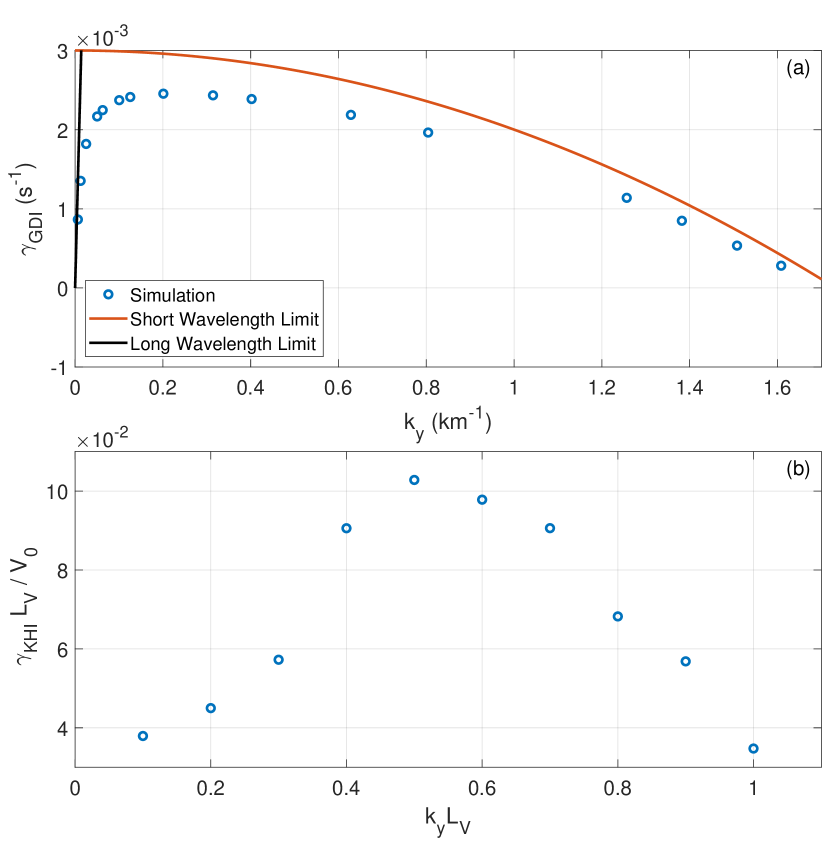
Figure 8: Plots of the growth rate as a function of wavenumber for single mode GDI (a) and KHI (b) simulations. Panel (a) shows the GDI growth rate, where the circles are the simulation growth rate, the red line is the short wavelength limit (Eq. 38), and the black line is the long wavelength limit (Eq. 39). The results indicate that the simulation growth rate tends to approach the appropriate limit as $k_{y}$ approaches 0 or $\infty$. Panel (b) shows the KHI growth rate calculated from the simulations. This growth rate is compared to Figure 3 from Ref. 17, showing reasonable agreement of the location of peak growth and magnitude of the growth rate.

The KHI simulations are run using $512\times 16$ grid points. Many of the KHI length parameters are based on the length $L_{V}$ from Eq. 19, which is used to obtain the background velocity profile, with $L_{V}=10$ km, $V_{0}=1000$ m/s, $x_{V_{1}}=4L_{V}$, and $x_{V_{2}}=8L_{V}$. The domain size is set to $20L_{V}\times 2\pi/k_{y}$, where $k_{y}$ is defined such that the value $k_{y}L_{V}$ is varied from 0.1 to 1.0. Eq. 18 is used for the density profile with $n_{0}=10^{11}$ $\mathrm{m}^{-3}$, $a_{1}=-1$, $a_{2}=1$, $c=1$, $x_{N_{1}}=4L_{V}$, $x_{N_{2}}=16L_{V}$, and $L_{N}=L_{V}$. The background neutral wind is set to 0. The background magnetic field is $B=$5\text{\times}{10}^{-5}\text{\,}\mathrm{T}$$. The neutral and ion species are atomic and ionic oxygen respectively, with a neutral number density of $n_{n}=10^{11}$ $\mathrm{m}^{-3}$, which corresponds to $R=$9.87\text{\times}{10}^{-8}$$. The numerical diffusion constant is $D=0$ $\mathrm{m}^{2}\mathrm{/}\mathrm{s}$.

Figure 8(b) shows the simulation growth rate, normalized by $V_{0}/L_{V}$, for the KHI as a function of the wavenumber, normalized by $L_{V}$. The normalized ion-neutral collision frequency is $\nu_{in}L_{V}/V_{0}=$2.96\text{\times}{10}^{-4}$$. This result can be compared to Figure 3 from Ref. 17. Note that due to the complicated nonlocal analysis, the growth rate does not have an analytical form[17]. Figure 8(b) shows that the location of peak growth in occurs at about $k_{y}L_{V}=0.5$ which is consistent with Figure 3 from Ref. 17. The magnitude of the growth rate is on the same order of magnitude as the results from Ref. 17. Thus, there is reasonable agreement between the simulation results and linear theory.

Thus, the GDI and KHI reasonably match linear theory in conditions that are already well understood. This paper shows that there are regimes which have not been studied in the literature. Future work constitutes conducting a nonlocal linear analysis to investigate, from a theoretical perspective, the GDI and the KHI in combination.

References

- Simon [1963] A. Simon, “Instability of a partially ionized plasma in crossed electric and magnetic fields,” The physics of fluids 6, 382–388 (1963).
- Hoh [1963] F. Hoh, “Instability of penning-type discharges,” The Physics of Fluids 6, 1184–1191 (1963).
- Fejer and Kelley [1980] B. G. Fejer and M. Kelley, “Ionospheric irregularities,” Reviews of Geophysics 18, 401–454 (1980).
- Keskinen and Ossakow [1983] M. Keskinen and S. Ossakow, “Theories of high-latitude ionospheric irregularities: A review,” Radio science 18, 1077–1091 (1983).
- Tsunoda [1988] R. T. Tsunoda, “High-latitude f region irregularities: A review and synthesis,” Reviews of Geophysics 26, 719–760 (1988).
- Linson and Workman [1970] L. M. Linson and J. B. Workman, “Formation of striations in ionospheric plasma clouds,” Journal of Geophysical Research 75, 3211–3219 (1970).
- Haerendel and Lüst [1968] G. Haerendel and R. Lüst, “Artificial plasma clouds in space,” Scientific American 219, 80–95 (1968).
- McDonald et al. [1980] B. McDonald, M. Keskinen, S. Ossakow, and S. Zalesak, “Computer simulation of gradient drift instability processes in operation avefria,” Journal of Geophysical Research: Space Physics 85, 2143–2154 (1980).
- Weber et al. [1984] E. J. Weber, J. Buchau, J. Moore, J. Sharber, R. Livingston, J. D. Winningham, and B. Reinisch, “F layer ionization patches in the polar cap,” Journal of Geophysical Research: Space Physics 89, 1683–1694 (1984).
- Moen et al. [2012] J. Moen, K. Oksavik, T. Abe, M. Lester, Y. Saito, T. Bekkeng, and K. Jacobsen, “First in-situ measurements of hf radar echoing targets,” Geophysical Research Letters 39 (2012).
- Lamarche and Makarevich [2017] L. J. Lamarche and R. A. Makarevich, “Radar observations of density gradients, electric fields, and plasma irregularities near polar cap patches in the context of the gradient-drift instability,” Journal of Geophysical Research: Space Physics 122, 3721–3736 (2017).
- Greenwald [1974] R. Greenwald, “Diffuse radar aurora and the gradient drift instability,” Journal of Geophysical Research 79, 4807–4810 (1974).
- Tsunoda and Vickrey [1982] R. T. Tsunoda and J. F. Vickrey, “Evidence of east-west structure in large-scale f-region plasma enhancements in the auroral zone.” Tech. Rep. (SRI INTERNATIONAL MENLO PARK CA, 1982).
- Sahr and Fejer [1996] J. D. Sahr and B. G. Fejer, “Auroral electrojet plasma irregularity theory and experiment: A critical review of present understanding and future directions,” Journal of Geophysical Research: Space Physics 101, 26893–26909 (1996).
- Chandrasekhar [1961] S. Chandrasekhar, Hydrodynamic and hydromagnetic stability (Oxford University Press, 1961).
- Kintner and Seyler [1985] P. M. Kintner and C. E. Seyler, “The status of observations and theory of high latitude ionospheric and magnetospheric plasma turbulence,” Space science reviews 41, 91–129 (1985).
- Keskinen et al. [1988] M. Keskinen, H. Mitchell, J. Fedder, P. Satyanarayana, S. Zalesak, and J. Huba, “Nonlinear evolution of the kelvin-helmholtz instability in the high-latitude ionosphere,” Journal of Geophysical Research: Space Physics 93, 137–152 (1988).
- Gondarenko and Guzdar [1999] N. Gondarenko and P. Guzdar, “Gradient drift instability in high latitude plasma patches: Ion inertial effects,” Geophysical research letters 26, 3345–3348 (1999).
- Perkins and Doles III [1975] F. Perkins and J. Doles III, “Velocity shear and the e b instability,” Journal of Geophysical Research 80, 211–214 (1975).
- Huba et al. [1983] J. Huba, S. Ossakow, P. Satyanarayana, and P. Guzdar, “Linear theory of the e b instability with an inhomogeneous electric field,” Journal of Geophysical Research: Space Physics 88, 425–434 (1983).
- Huba and Lee [1983] J. D. Huba and L. Lee, “Short wavelength stabilization of the gradient drift instability due to velocity shear,” Geophysical research letters 10, 357–360 (1983).
- Rathod et al. [2020] C. Rathod, B. Srinivasan, W. A. Scales, and B. S. R. Kunduri, “Investigation of the gradient drift instability as a cause of density irregularities in subauroral polarization streams,” (2020), https://doi.org/10.1002/essoar.10504471.1.
- Dang et al. [2020] T. Dang, B. Zhang, J. Lei, W. Wang, A. Burns, H.-l. Liu, K. Pham, and K. A. Sorathia, “Development of high-resolution thermosphere–ionosphere electrodynamics general circulation model (tie-gcm) using ring average technique,” Geoscientific Model Development Discussions , 1–30 (2020).
- Foster and Burke [2002] J. Foster and W. Burke, “Saps: A new categorization for sub-auroral electric fields,” Eos, Transactions American Geophysical Union 83, 393–394 (2002).
- Spiro, Heelis, and Hanson [1978] R. Spiro, R. Heelis, and W. Hanson, “Ion convection and the formation of the mid-latitude f region ionization trough,” Journal of Geophysical Research: Space Physics 83, 4255–4264 (1978).
- Ledvina, Makela, and Kintner [2002] B. Ledvina, J. J. Makela, and P. Kintner, “First observations of intense gps l1 amplitude scintillations at midlatitude,” Geophysical Research Letters 29, 4–1 (2002).
- Mishin et al. [2003] E. Mishin, W. Burke, C. Huang, and F. Rich, “Electromagnetic wave structures within subauroral polarization streams,” Journal of Geophysical Research: Space Physics 108 (2003).
- Foster et al. [2004] J. Foster, P. Erickson, F. Lind, and W. Rideout, “Millstone hill coherent-scatter radar observations of electric field variability in the sub-auroral polarization stream,” Geophysical research letters 31 (2004).
- Oksavik et al. [2006] K. Oksavik, R. Greenwald, J. Ruohoniemi, M. Hairston, L. Paxton, J. Baker, J. Gjerloev, and R. Barnes, “First observations of the temporal/spatial variation of the sub-auroral polarization stream from the superdarn wallops hf radar,” Geophysical research letters 33 (2006).
- Mishin and Blaunstein [2008] E. Mishin and N. Blaunstein, “Irregularities within subauroral polarization stream-related troughs and gps radio interference at midlatitudes,” Midlatitude Ionospheric Dynamics and Disturbances, Geophys. Monogr. Ser 181, 291–295 (2008).
- Keskinen and Ossakow [1982] M. J. Keskinen and S. Ossakow, “Nonlinear evolution of plasma enhancements in the auroral ionosphere, 1, long wavelength irregularities,” Journal of Geophysical Research: Space Physics 87, 144–150 (1982).
- Makarevich [2014] R. A. Makarevich, “Symmetry considerations in the two-fluid theory of the gradient drift instability in the lower ionosphere,” Journal of Geophysical Research: Space Physics 119, 7902–7913 (2014).
- Ossakow, Chaturvedi, and Workman [1978] S. Ossakow, P. Chaturvedi, and J. Workman, “High-altitude limit of the gradient drift instability,” Journal of Geophysical Research: Space Physics 83, 2691–2693 (1978).
- Makarevich [2019] R. A. Makarevich, “Toward an integrated view of ionospheric plasma instabilities: 3. explicit growth rate and oscillation frequency for arbitrary altitude,” Journal of Geophysical Research: Space Physics 124, 6138–6155 (2019).
- Wang, Ye, and Li [2010] L. Wang, W. Ye, and Y. Li, “Combined effect of the density and velocity gradients in the combination of kelvin–helmholtz and rayleigh–taylor instabilities,” Physics of Plasmas 17, 042103 (2010).
- Hysell and Kudeki [2004] D. Hysell and E. Kudeki, “Collisional shear instability in the equatorial f region ionosphere,” Journal of Geophysical Research: Space Physics 109 (2004).
- Hudson and Kelley [1976] M. K. Hudson and M. C. Kelley, “The temperature gradient drift instability at the equatorward edge of the ionospheric plasma trough,” Journal of Geophysical Research 81, 3913–3918 (1976).
- Keskinen, Basu, and Basu [2004] M. Keskinen, S. Basu, and S. Basu, “Midlatitude sub-auroral ionospheric small scale structure during a magnetic storm,” Geophysical research letters 31 (2004).
- Canuto et al. [2012] C. Canuto, M. Y. Hussaini, A. Quarteroni, and A. Thomas Jr, Spectral methods in fluid dynamics (Springer Science & Business Media, 2012).
- Hirsch [1990] C. Hirsch, Numerical Computation of Internal and External Flows: Volume 2: Computational Methods for Inviscid and Viscous Flow (Wiley & Sons, 1990).
- Mitchell Jr et al. [1985] H. Mitchell Jr, J. Fedder, M. Keskinen, and S. Zalesak, “A simulation of high latitude f-layer instabilities in the presence of magnetosphere-ionosphere coupling,” Geophysical research letters 12, 283–286 (1985).
- Anderson, Heelis, and Hanson [1991] P. Anderson, R. Heelis, and W. Hanson, “The ionospheric signatures of rapid subauroral ion drifts,” Journal of Geophysical Research: Space Physics 96, 5785–5792 (1991).
- Buonsanto [1999] M. J. Buonsanto, “Ionospheric storms—a review,” Space Science Reviews 88, 563–601 (1999).
- Bilitza [2018] D. Bilitza, “Iri the international standard for the ionosphere.” Advances in Radio Science 16 (2018).
- Picone et al. [2002] J. Picone, A. Hedin, D. P. Drob, and A. Aikin, “Nrlmsise-00 empirical model of the atmosphere: Statistical comparisons and scientific issues,” Journal of Geophysical Research: Space Physics 107, SIA–15 (2002).
- Thébault et al. [2015] E. Thébault, C. C. Finlay, C. D. Beggan, P. Alken, J. Aubert, O. Barrois, F. Bertrand, T. Bondar, A. Boness, L. Brocco, et al., “International geomagnetic reference field: the 12th generation,” Earth, Planets and Space 67, 79 (2015).
- Bondi [1964] A. v. Bondi, “van der waals volumes and radii,” The Journal of physical chemistry 68, 441–451 (1964).
- Batsanov [2001] S. Batsanov, “Van der waals radii of elements,” Inorganic materials 37, 871–885 (2001).
- Chisham et al. [2007] G. Chisham, M. Lester, S. Milan, M. Freeman, W. Bristow, A. Grocott, K. McWilliams, J. Ruohoniemi, T. Yeoman, P. L. Dyson, et al., “A decade of the super dual auroral radar network (superdarn): Scientific achievements, new techniques and future directions,” Surveys in geophysics 28, 33–109 (2007).
- Huba and Zalesak [1983] J. Huba and S. Zalesak, “Long-wavelength limit of the e b instability,” Journal of Geophysical Research: Space Physics 88, 10263–10265 (1983).