Noisy quantum metrology
with the assistance of indefinite causal order

Abstract

A generic qubit unitary operator affected by depolarizing noise is duplicated and inserted in a quantum switch process realizing a superposition of causal orders. The characterization of the resulting switched quantum channel is worked out for its action on the joint state of the probe-control qubit pair. The switched channel is then specifically investigated for the important metrological task of phase estimation on the noisy unitary operator, with the performance assessed by the Fisher information, classical or quantum. A comparison is made with conventional techniques of estimation where the noisy unitary is directly probed in a one-stage or two-stage cascade with definite order, or several uses of them with two or more qubits. In the switched channel with indefinite order, specific properties are reported, meaningful for estimation and not present with conventional techniques. It is shown that the control qubit, although it never directly interacts with the unitary, can nevertheless be measured alone for effective estimation, while discarding the probe qubit that interacts with the unitary. Also, measurement of the control qubit maintains the possibility of efficient estimation in difficult conditions where conventional estimation becomes less efficient, as for instance with ill-configured input probes, or in blind situations when the axis of the unitary is unknown. Especially, effective estimation by measuring the control qubit remains possible even when the input probe tends to align with the axis of the unitary, or with a fully depolarized input probe, while in these conditions conventional estimation becomes inoperative. Measurement of the probe qubit of the switched channel is also analyzed and shown to add useful capabilities for phase estimation. The results contribute to the ongoing identification and analysis of the properties and capabilities of switched quantum channels with indefinite order for information processing, and uncover new possibilities for quantum estimation and qubit metrology.

1 Introduction

Quantum channels can be viewed as building blocks for performing quantum information processing by transforming quantum states or signals, much like in classical systems-and-signals theory. Two quantum channels (1) and (2) can be combined or cascaded, in the order (1)–(2) or (2)–(1), under the control of a quantum switch signal realized for instance by the two basis states of a qubit. Such a control qubit can be placed in an arbitrary superposition of its two basis states, and as a result, the two individual channels get cascaded in an arbitrary superposition of the two classical orders (1)–(2) or (2)–(1). This realizes a switched quantum channel formed by the two individual channels simultaneously cascaded in the two alternative orders, or with indefinite causal order. Such switched quantum channels with indefinite causal order are specifically quantum devices, grounded on quantum superposition, and with no classical analogue. Their principle has been described recently in [1, 2] and their physical implementation is addressed in [2, 3, 4, 5, 6, 7]. For information processing, it is being found that switched quantum channels with indefinite causal order can specifically offer useful capabilities, not accessible with channels combined in definite causal orders. Such specific capabilities from switched indefinite causal order have been reported with various channels and information processing tasks, assessed by appropriate efficiency metrics.

For instance, Refs. [8, 9, 10, 11] address a task of quantum communication of information, where typically isolated communication channels with limited capacity, when inserted in a quantum switch process, give rise to a switched quantum channel with enhanced capacity to transmit information. The task in [12, 13] is quantum channel discrimination; in [12] two channels that when associated in definite order are never perfectly distinguishable become so with indefinite order; in [13] for distinguishing whether or not a qubit has been affected by a given unitary transformation in the presence of noise, the probability of discrimination error is shown improvable by the quantum switch process. Very recently, switched channels with indefinite order have been extended to quantum metrological tasks involving parameter estimation from measurements [14, 15, 16]. It has been shown that a one-parameter quantum channel can be identified or estimated more efficiently when it is involved in a switch process, for a qudit depolarizing channel in [14] and a qubit thermalization channel in [15]. In [16], to estimate the product of two average displacements in a continuous-variable quantum system, it is shown that the estimation error can be reduced by the switch process.

Quantum switching with indefinite causal order is a phenomenon of recent introduction, and its properties and capabilities for information processing are still being inventoried and analyzed. In the present paper, we will extend the investigation of switched causal orders for quantum metrology, applied here to new quantum processes or channels and in different conditions. We will address the important task of quantum metrology consisting in parameter estimation on a unitary transformation in the presence of noise [17, 18, 19]. For quantum metrology, the switched processes considered here are different from those of [14, 15, 16], and the presence of noise is a significant specificity here. The Fisher information will be used to assess the performance for estimation, as in [14, 15, 16]; the Fisher information being a fundamental reference metric in metrology, often employed for characterization and fixing the best conceivable performance [20, 21].

In this paper, we will first briefly review the principle of the quantum switch of elementary channels. Then, from an elementary channel formed by a generic qubit unitary operator affected by depolarizing noise, we will carry out a complete characterization of the transformation realized by the corresponding switched quantum channel, specially by means of the Bloch representation of the qubit density operator. We will then concentrate on the important metrological task of estimating the phase parameter of the unitary operator, and evaluate the Fisher information to assess the performance. We will show the possibility of useful properties for the phase estimation with indefinite causal order in the switched unitary channel with noise. Especially, conditions will be reported where the switched channel with indefinite order remains efficient for estimation, while conventional techniques with definite order become inoperative. The study in this way will extend the analysis of switched channels with indefinite causal order to the task of estimation on a noisy qubit unitary, and will report new possibilities to contribute to quantum estimation and qubit metrology.

2 Quantum switch of two quantum channels

We consider as in [2, 8], acting on quantum systems with Hilbert space $\mathcal{H}$, a quantum channel (1) with Kraus operators $\bigl{\{}\mathsf{K}_{k}^{(1)}\bigr{\}}$ and a second quantum channel (2) with Kraus operators $\bigl{\{}\mathsf{K}_{j}^{(2)}\bigr{\}}$. The two channels are cascaded either in the order (1)–(2) or (2)–(1), under the control of a qubit driving a quantum switch process as described for instance in [2, 8]. When the control qubit is in state $\mathinner{|{0}\rangle}$ channel (1) is traversed first, followed by channel (2); and when the control qubit is in state $\mathinner{|{1}\rangle}$ channel (2) is traversed first, followed by channel (1), as depicted in Fig. 1.

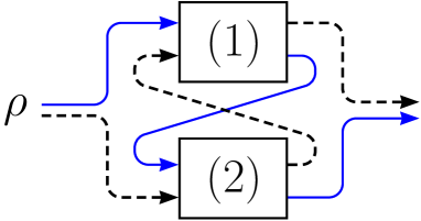
Figure 1: Two quantum channels (1) and (2) can be cascaded either in the order (1)–(2) (solid path) or (2)–(1) (dashed path) according to the state respectively $\mathinner{|{0}\rangle}$ or $\mathinner{|{1}\rangle}$ of a control qubit.

The resulting “switched” quantum channel is described [2, 8] by the Kraus operators

$$\mathsf{K}_{jk}=\mathsf{K}_{j}^{(2)}\mathsf{K}_{k}^{(1)}\otimes\mathinner{|{0}\rangle}\mathinner{\langle{0}|}_{c}+\mathsf{K}_{k}^{(1)}\mathsf{K}_{j}^{(2)}\otimes\mathinner{|{1}\rangle}\mathinner{\langle{1}|}_{c}\;.$$ (1)

When acting on a quantum state of $\mathcal{H}$ with density operator $\rho$ along with a control qubit in state $\rho_{c}$, the switched quantum channel implements the bipartite quantum operation $\mathcal{S}$ defined [2, 8] by the superoperator

$$\mathcal{S}(\rho\otimes\rho_{c})=\sum_{j,k}\mathsf{K}_{jk}(\rho\otimes\rho_{c})\mathsf{K}_{jk}^{\dagger}\;.$$ (2)

The quantum operation realized in Eq. (2) can be further developed as

$$\mathcal{S}(\rho\otimes\rho_{c}) = \mathcal{S}_{00}(\rho)\otimes\mathinner{\langle{0|\rho_{c}|0}\rangle}\mathinner{|{0}\rangle}\mathinner{\langle{0}|}_{c}+\mathcal{S}_{01}(\rho)\otimes\mathinner{\langle{0|\rho_{c}|1}\rangle}\mathinner{|{0}\rangle}\mathinner{\langle{1}|}_{c}$$

$$+ \mathcal{S}_{01}^{\dagger}(\rho)\otimes\mathinner{\langle{1|\rho_{c}|0}\rangle}\mathinner{|{1}\rangle}\mathinner{\langle{0}|}_{c}+\mathcal{S}_{11}(\rho)\otimes\mathinner{\langle{1|\rho_{c}|1}\rangle}\mathinner{|{1}\rangle}\mathinner{\langle{1}|}_{c}\;,$$ (3)

with the superoperators

$$\mathcal{S}_{00}(\rho) = \sum_{j,k}\mathsf{K}_{j}^{(2)}\mathsf{K}_{k}^{(1)}\rho\mathsf{K}_{k}^{(1)\dagger}\mathsf{K}_{j}^{(2)\dagger}\;,$$ (4)

$$\mathcal{S}_{01}(\rho) = \sum_{j,k}\mathsf{K}_{j}^{(2)}\mathsf{K}_{k}^{(1)}\rho\mathsf{K}_{j}^{(2)\dagger}\mathsf{K}_{k}^{(1)\dagger}\;,$$ (5)

$$\mathcal{S}_{11}(\rho) = \sum_{j,k}\mathsf{K}_{k}^{(1)}\mathsf{K}_{j}^{(2)}\rho\mathsf{K}_{j}^{(2)\dagger}\mathsf{K}_{k}^{(1)\dagger}\;.$$ (6)

The superoperator $\mathcal{S}_{00}(\rho)$ alone describes the quantum operation realized by the standard cascade with the definite causal order (1)–(2), and similarly with $\mathcal{S}_{11}(\rho)$ for the cascade (2)–(1). By contrast, the superoperator $\mathcal{S}_{01}(\rho)$ is a coupling term specific to the quantum switch process. In the joint state $\mathcal{S}(\rho\otimes\rho_{c})$ of Eq. (3), if the control qubit were discarded (unobserved) and traced out, the resulting quantum operation on $\rho$ would represent a classical probabilistic (convex) combination of the two definite causal orders $\mathcal{S}_{00}(\rho)$ and $\mathcal{S}_{11}(\rho)$. By contrast, if the control qubit is treated coherently with $\rho$ it can give rise to specific, specifically quantum, behaviors from the switched quantum channel, as we shall see.

An interesting and specifically quantum feature is that the control qubit can be placed in the superposed state $\mathinner{|{\psi_{c}}\rangle}=\sqrt{p_{c}}\mathinner{|{0}\rangle}+\sqrt{1-p_{c}}\mathinner{|{1}\rangle}$, with $p_{c}\in[0,1]$. This produces in Eqs. (2)–(3) a switched quantum channel representing a quantum superposition of the two initial channels (1) and (2) simultaneously cascaded in the two alternative orders, or with indefinite causal order. With $\rho_{c}=\mathinner{|{\psi_{c}}\rangle}\mathinner{\langle{\psi_{c}}|}$, the quantum operation resulting in Eq. (3) takes the form

$$\mathcal{S}(\rho\otimes\rho_{c}) = p_{c}\mathcal{S}_{00}(\rho)\otimes\mathinner{|{0}\rangle}\mathinner{\langle{0}|}_{c}+(1-p_{c})\mathcal{S}_{11}(\rho)\otimes\mathinner{|{1}\rangle}\mathinner{\langle{1}|}_{c}$$

$$+ \sqrt{(1-p_{c})p_{c}}\bigl{[}\mathcal{S}_{01}(\rho)\otimes\mathinner{|{0}\rangle}\mathinner{\langle{1}|}_{c}+\mathcal{S}_{01}^{\dagger}(\rho)\otimes\mathinner{|{1}\rangle}\mathinner{\langle{0}|}_{c}\bigr{]}\;.$$ (7)

We will consider the situation where the quantum channels (1) and (2) are qubit channels, under a form which is often encountered in quantum metrology, and consisting in a unitary operator $\mathsf{U}_{\xi}$ affected by a quantum noise $\mathcal{N}(\cdot)$.

3 A unitary qubit channel with noise

For qubits with two-dimensional Hilbert space $\mathcal{H}_{2}$, the density operator is represented in Bloch representation [22] under the form

$$\rho=\frac{1}{2}\bigl{(}\mathrm{I}_{2}+\vec{r}\cdot\vec{\sigma}\bigr{)}\;,$$ (8)

where $\mathrm{I}_{2}$ is the identity operator on $\mathcal{H}_{2}$, and $\vec{\sigma}$ a formal vector assembling the three (traceless Hermitian unitary) Pauli operators $[\sigma_{x},\sigma_{y},\sigma_{z}]=\vec{\sigma}$. The Bloch vector $\vec{r}\in\mathbbm{R}^{3}$ characterizing the density operator has norm $\|\vec{r}\,\|=1$ for a pure state, and $\|\vec{r}\,\|<1$ for a mixed state.

A qubit unitary operator $\mathsf{U}_{\xi}$ is introduced with the general parameterization [22]

$$\mathsf{U}_{\xi}=\exp\Bigl{(}-i\frac{\displaystyle\xi}{\displaystyle 2}\vec{n}\cdot\vec{\sigma}\Bigr{)}=\cos\Bigl{(}\frac{\xi}{2}\Bigr{)}\,\mathrm{I}_{2}-i\sin\Bigl{(}\frac{\xi}{2}\Bigr{)}\,\vec{n}\cdot\vec{\sigma}\;,$$ (9)

where $\vec{n}=[n_{x},n_{y},n_{z}]^{\top}$ is a unit vector of $\mathbbm{R}^{3}$, and $\xi$ a phase angle in $[0,2\pi)$.

From a qubit state $\rho$ in Bloch representation as in Eq. (8), the unitary $\mathsf{U}_{\xi}$ produces the transformed state

$$\mathsf{U}_{\xi}\rho\mathsf{U}_{\xi}^{\dagger}=\frac{1}{2}\bigl{(}\mathrm{I}_{2}+U_{\xi}\vec{r}\cdot\vec{\sigma}\bigr{)}\;,$$ (10)

which amounts to the transformation $U_{\xi}\vec{r}$ of the Bloch vector $\vec{r}$ in $\mathbbm{R}^{3}$ experiencing a rotation around the axis $\vec{n}$ by the angle $\xi$ via the $3\times 3$ real matrix

$$U_{\xi}=\begin{bmatrix}\cos(\xi)+[1-\cos(\xi)]n_{x}^{2}&[1-\cos(\xi)]n_{x}n_{y}-\sin(\xi)n_{z}&[1-\cos(\xi)]n_{x}n_{z}+\sin(\xi)n_{y}\\ [1-\cos(\xi)]n_{x}n_{y}+\sin(\xi)n_{z}&\cos(\xi)+[1-\cos(\xi)]n_{y}^{2}&[1-\cos(\xi)]n_{y}n_{z}-\sin(\xi)n_{x}{\vrule height=17.07164pt,depth=0.0pt,width=0.0pt}\\ [1-\cos(\xi)]n_{x}n_{z}-\sin(\xi)n_{y}&[1-\cos(\xi)]n_{y}n_{z}+\sin(\xi)n_{x}&\cos(\xi)+[1-\cos(\xi)]n_{z}^{2}{\vrule height=17.07164pt,depth=0.0pt,width=0.0pt}\end{bmatrix}.$$ (11)

The qubit noise $\mathcal{N}(\cdot)$ is introduced under the form of a depolarizing noise [22] implementing the quantum operation with Kraus representation

$$\mathcal{N}(\rho)=(1-p)\rho+\frac{\displaystyle p}{\displaystyle 3}\bigl{(}\sigma_{x}\rho\sigma_{x}^{\dagger}+\sigma_{y}\rho\sigma_{y}^{\dagger}+\sigma_{z}\rho\sigma_{z}^{\dagger}\bigr{)}\;.$$ (12)

The effect of the noise in Eq. (12) is to leave the qubit state $\rho$ unchanged with the probability $1-p$ or to apply any one of the three Pauli operators with equal probability $p/3$. Alternatively, the effect of the depolarizing noise can be described, for the Bloch vector $\vec{r}$ characterizing a qubit state in Eq. (8), as the isotropic compression $\vec{r}\mapsto\alpha\vec{r}$ with the compression factor $\alpha=1-4p/3$. Equivalently, Eq. (12) is also

$$\mathcal{N}(\rho)=\alpha\rho+(1-\alpha)\frac{\mathrm{I}_{2}}{2}\;,$$ (13)

indicating that with the probability $1-\alpha$, the noise replaces the quantum state $\rho$ by the maximally mixed state $\mathrm{I}_{2}/2$; at the maximum compression when $\alpha=0$ the quantum state is forced to $\mathrm{I}_{2}/2$ with probability $1$ and the qubit gets completely depolarized. The depolarizing noise is an important noise model often considered in quantum information [22]. It has no invariant subspace, and in this respect it represents in some sense a worse-case noise and as such a conservative reference. Here, in addition, its isotropic character will ease the theoretical derivations. However, this choice for the type of noise is not critical for the main properties to be reported here.

The quantum channel like (1) or (2) of Section 2 is formed by cascading the unitary transformation $\mathsf{U}_{\xi}$ of Eq. (9) and the depolarizing noise $\mathcal{N}(\cdot)$ of Eqs. (12)–(13), as depicted in Fig. 2.

Figure 2: A qubit channel formed by the unitary transformation $\mathsf{U}_{\xi}$ of Eq. (9) and the depolarizing noise $\mathcal{N}(\cdot)$ of Eqs. (12)–(13). As a whole this channel is an instance of channel (1) or (2) considered in Fig. 1.

For the quantum channel of Fig. 2, four Kraus operators like $\mathsf{K}_{k}^{(1)}$ or $\mathsf{K}_{j}^{(2)}$ of Section 2 result as $\bigl{\{}\mathsf{K}_{0}=\sqrt{1-p}\mathsf{U}_{\xi},\mathsf{K}_{1}=\sqrt{p/3}\sigma_{x}\mathsf{U}_{\xi},\mathsf{K}_{2}=\sqrt{p/3}\sigma_{y}\mathsf{U}_{\xi},\mathsf{K}_{3}=\sqrt{p/3}\sigma_{z}\mathsf{U}_{\xi}\bigr{\}}$. Equivalently, for a qubit state $\rho$ in Bloch representation as in Eq. (8), the cascade of $\mathsf{U}_{\xi}$ then $\mathcal{N}(\cdot)$ produces the transformed state

$$\mathcal{N}(\mathsf{U}_{\xi}\rho\mathsf{U}_{\xi}^{\dagger})=\frac{1}{2}\bigl{(}\mathrm{I}_{2}+\alpha U_{\xi}\vec{r}\cdot\vec{\sigma}\bigr{)}\;.$$ (14)

We note that, although the four Kraus operators $\mathsf{K}_{j}$ above generally do not commute between them, as a whole the isotropic depolarizing noise $\mathcal{N}(\cdot)$ here commutes with the unitary $\mathsf{U}_{\xi}$ in Fig. 2, so that $\mathcal{N}(\mathsf{U}_{\xi}\rho\mathsf{U}_{\xi}^{\dagger})$ in Eq. (14) coincides with $\mathsf{U}_{\xi}\mathcal{N}(\rho)\mathsf{U}_{\xi}^{\dagger}$. The noise action $\mathcal{N}(\cdot)$ is placed after $\mathsf{U}_{\xi}$ in Fig. 2, but it could as well take place before $\mathsf{U}_{\xi}$, or even part before and part after $\mathsf{U}_{\xi}$ and equivalently lumped into a single action as in Fig. 2.

4 Quantum switch of two noisy unitaries

Two such identical qubit channels formed by $\mathsf{U}_{\xi}$ and $\mathcal{N}(\cdot)$ as in Fig. 2 are associated as in Fig. 1 through the quantum switch process of Section 2, with however two independent noise sources according to Eqs. (12)–(13) at a same noise level $p$ or $\alpha$. For two identical channels (1) and (2), one has $\mathcal{S}_{00}(\rho)=\mathcal{S}_{11}(\rho)$ in Eqs. (4), (6), and also $\mathcal{S}_{01}^{\dagger}(\rho)=\mathcal{S}_{01}(\rho)$ in Eq. (5). On the probe qubit in state $\rho$ and control qubit in state $\rho_{c}=\mathinner{|{\psi_{c}}\rangle}\mathinner{\langle{\psi_{c}}|}$, the switched quantum channel therefore realizes the two-qubit quantum operation from Eq. (7) reading

$$\mathcal{S}(\rho\otimes\rho_{c}) = \mathcal{S}_{00}(\rho)\otimes\bigl{[}p_{c}\mathinner{|{0}\rangle}\mathinner{\langle{0}|}_{c}+(1-p_{c})\mathinner{|{1}\rangle}\mathinner{\langle{1}|}_{c}\bigr{]}$$ (15)

$$+ \mathcal{S}_{01}(\rho)\otimes\sqrt{(1-p_{c})p_{c}}\bigl{(}\mathinner{|{0}\rangle}\mathinner{\langle{1}|}_{c}+\mathinner{|{1}\rangle}\mathinner{\langle{0}|}_{c}\bigr{)}\;.$$

Furthermore, as already mentioned, from Eq. (4) it can be verified that $\mathcal{S}_{00}(\rho)$ (and $\mathcal{S}_{11}(\rho)$ similarly) is simply the quantum operation realized on $\rho$ by directly traversing in a standard cascade with definite order the two channels (1) then (2), which in Bloch representation via Eq. (14) amounts to

$$\mathcal{S}_{00}(\rho)=\frac{1}{2}\bigl{(}\mathrm{I}_{2}+\alpha^{2}U_{\xi}^{2}\vec{r}\cdot\vec{\sigma}\bigr{)}\;.$$ (16)

For the superoperator $\mathcal{S}_{01}(\rho)$ of Eq. (5) one has now

$$\mathcal{S}_{01}(\rho) = (1-p)^{2}\mathcal{W}_{0}+(1-p)\frac{\displaystyle p}{\displaystyle 3}\sum_{\ell=x,y,z}\bigl{(}\mathcal{W}_{\ell}+\mathcal{W}_{\ell}^{\dagger}\bigr{)}+\Bigl{(}\frac{\displaystyle p}{\displaystyle 3}\Bigr{)}^{2}\Bigl{[}$$ (17)

$$\bigl{(}\mathcal{W}_{xy}+\mathcal{W}_{xy}^{\dagger}\bigr{)}+\bigl{(}\mathcal{W}_{yz}+\mathcal{W}_{yz}^{\dagger}\bigr{)}+\bigl{(}\mathcal{W}_{zx}+\mathcal{W}_{zx}^{\dagger}\bigr{)}+\mathcal{W}_{xx}+\mathcal{W}_{yy}+\mathcal{W}_{zz}\Bigr{]}\;,$$

with the superoperators

$$\mathcal{W}_{0}(\rho) = \mathsf{U}_{\xi}^{2}\rho\mathsf{U}_{\xi}^{\dagger 2}\;,$$ (18)

$$\mathcal{W}_{\ell}(\rho) = \sigma_{\ell}\mathsf{U}_{\xi}\mathsf{U}_{\xi}\rho\mathsf{U}_{\xi}^{\dagger}\sigma_{\ell}^{\dagger}\mathsf{U}_{\xi}^{\dagger}\;,$$ (19)

$$\mathcal{W}_{\ell\ell^{\prime}}(\rho) = \sigma_{\ell}\mathsf{U}_{\xi}\sigma_{\ell^{\prime}}\mathsf{U}_{\xi}\rho\mathsf{U}_{\xi}^{\dagger}\sigma_{\ell}^{\dagger}\mathsf{U}_{\xi}^{\dagger}\sigma_{\ell^{\prime}}^{\dagger}\;,$$ (20)

verifying that $\mathcal{S}_{01}(\rho)=\mathcal{S}_{01}^{\dagger}(\rho)$. In Eq. (19) and comparable equations, $\sigma_{\ell}$ designates generically one of the three Pauli operators $\sigma_{x}$, $\sigma_{y}$ or $\sigma_{z}$ according to the value of $\ell$. What we want to do next, is to characterize the action of the superoperator $\mathcal{S}_{01}(\rho)$ of Eq. (17) by means of the Bloch representation, as in Eq. (16). This can be carried out in two steps, by expressing $\mathcal{S}_{01}(\mathrm{I}_{2})$ and $\mathcal{S}_{01}(\vec{r}\cdot\vec{\sigma})$. These derivations are developed in Appendix A.

From Appendix A, its Eq. (A-12), we obtain

$$\mathcal{S}_{01}(\mathrm{I}_{2})=\biggl{[}\frac{\displaystyle 4}{\displaystyle 3}p\Bigl{(}1-\frac{\displaystyle 4}{\displaystyle 3}p\Bigr{)}\cos(\xi)+1-\frac{\displaystyle 4}{\displaystyle 3}p\Bigl{(}1-\frac{\displaystyle p}{\displaystyle 3}\Bigr{)}\biggr{]}\mathrm{I}_{2}\;,$$ (21)

and from its Eq. (A-33),

$$\mathcal{S}_{01}(\vec{r}\cdot\vec{\sigma})=\Bigl{[}(1-p)^{2}U_{\xi}+(1-p)\frac{\displaystyle p}{\displaystyle 3}2\bigl{[}I_{3}+L_{1}(U_{\xi})\bigr{]}+\Bigl{(}\frac{\displaystyle p}{\displaystyle 3}\Bigr{)}^{2}\bigl{[}2L_{2}(U_{\xi})-2I_{3}+L_{3}(U_{\xi})\bigr{]}\Bigr{]}U_{\xi}\vec{r}\cdot\vec{\sigma}\;.$$ (22)

This completes the characterization of the joint two-qubit state $\mathcal{S}(\rho\otimes\rho_{c})$ of Eq. (15) produced by the switched quantum channel. It follows in particular that, when there is no noise, at $p=0$ in Eq. (12), the characterization leads to a joint state reducing to $\mathcal{S}(\rho\otimes\rho_{c})=\bigl{(}\mathsf{U}_{\xi}^{2}\rho\mathsf{U}_{\xi}^{\dagger 2}\bigr{)}\otimes\rho_{c}$, indicating that the two qubits evolve separately. The probe qubit in state $\rho$ experiences the standard unitary cascade $\mathsf{U}_{\xi}\mathsf{U}_{\xi}$, while the control qubit in state $\rho_{c}$ remains unaffected. This situation can be understood because with no noise the two channels that are switched are two strictly identical unitaries $\mathsf{U}_{\xi}$, so that the two switched orders $\mathsf{U}_{\xi}\mathsf{U}_{\xi}$ and $\mathsf{U}_{\xi}\mathsf{U}_{\xi}$ in Fig. 1 are identical and indistinguishable. The resulting switched channel is indistinguishable from a standard cascade of two unitaries $\mathsf{U}_{\xi}$. There is no superposition of two distinguishable causal orders, but only a standard cascade with definite order. By contrast, in the presence of noise, at $p\not=0$ in Eq. (12), the joint state $\mathcal{S}(\rho\otimes\rho_{c})$ of Eq. (15) is an entangled state, expressing a coupling evolution of the probe-control qubit pair. The two channels according to Fig. 2 engaged in the switch process of Fig. 1, do not reduce to a standard cascade of two indistinguishable channels. Indistinguishability of the two switched channels in Fig. 1 can be attributed to their Kraus operators which do not commute, as in [8]. The nonunitary noise process $\mathcal{N}(\cdot)$ shown in Fig. 2, which occurs in two independent realizations, involves in Eq. (12) Kraus operators which do not commute, so that the Kraus operators $\mathsf{K}_{k}^{(1)}$ or $\mathsf{K}_{j}^{(2)}$ of the two switched channels of Fig. 2 also do not commute. This induces in Fig. 1 a superposition of two distinguishable causal orders, and an entangling interaction of the two qubits, mediated via a nontrivial coupling term $\mathcal{S}_{01}(\rho)$ in the joint state $\mathcal{S}(\rho\otimes\rho_{c})$ of Eq. (15).

We will now examine the exploitation of the joint state $\mathcal{S}(\rho\otimes\rho_{c})$ of Eq. (15) characterizing the switched channel, to serve in a task of parameter estimation on the unitary $\mathsf{U}_{\xi}$.

5 Measurement

The probe qubit prepared in state $\rho$ and the control qubit prepared in state $\rho_{c}$ get entangled by the action of the switched quantum channel, and these two qubits together terminate in the joint state $\mathcal{S}(\rho\otimes\rho_{c})$ of Eq. (15). To extract information from the switched channel, a useful strategy, also adopted for instance in [8], is to measure the control qubit in the Fourier basis $\bigl{\{}\mathinner{|{+}\rangle},\mathinner{|{-}\rangle}\bigr{\}}$ of $\mathcal{H}_{2}$. The measurement can be described by the two measurement operators $\bigl{\{}\mathrm{I}_{2}\otimes\mathinner{|{+}\rangle}\mathinner{\langle{+}|},\mathrm{I}_{2}\otimes\mathinner{|{-}\rangle}\mathinner{\langle{-}|}\bigr{\}}$ acting in the Hilbert space $\mathcal{H}_{2}\otimes\mathcal{H}_{2}$ of the probe-control qubit pair with state $\mathcal{S}(\rho\otimes\rho_{c})$. The measurement randomly projects the control qubit either in state $\mathinner{|{+}\rangle}$ or $\mathinner{|{-}\rangle}$, and it leaves the probe qubit in the unnormalized conditional state

$$\rho_{\pm}={}_{c}\langle\pm|\mathcal{S}(\rho\otimes\rho_{c})|\pm\rangle_{c}=\frac{\displaystyle 1}{\displaystyle 2}\mathcal{S}_{00}(\rho)\pm\sqrt{(1-p_{c})p_{c}}\,\mathcal{S}_{01}(\rho)\;,$$ (23)

the products involving $\mathinner{|{\pm}\rangle}_{c}$ being defined on the control qubit. The probabilities $P^{\rm con}_{\pm}$ of the two measurement outcomes are provided by the trace $P^{\rm con}_{\pm}=\operatorname{tr}(\rho_{\pm})$. When the probe qubit is prepared in the state $\rho$ of Eq. (8), one has

$$\operatorname{tr}(\rho_{\pm})=\frac{\displaystyle 1}{\displaystyle 2}\operatorname{tr}\biggl{[}\frac{\displaystyle 1}{\displaystyle 2}\mathcal{S}_{00}(\mathrm{I}_{2})\pm\sqrt{(1-p_{c})p_{c}}\,\mathcal{S}_{01}(\mathrm{I}_{2})\biggr{]}\;,$$ (24)

since according to Eqs. (16) and (22) the terms $\mathcal{S}_{00}(\vec{r}\cdot\vec{\sigma})=\alpha^{2}U_{\xi}^{2}\vec{r}\cdot\vec{\sigma}$ and $\mathcal{S}_{01}(\vec{r}\cdot\vec{\sigma})$ are both linear combinations of the three Pauli operators $\vec{\sigma}$ and are therefore with zero trace. Via Eq. (16) giving $\mathcal{S}_{00}(\mathrm{I}_{2})=\mathrm{I}_{2}$ and Eq. (21) for $\mathcal{S}_{01}(\mathrm{I}_{2})$, one then obtains for the control qubit the measurement probabilities

$$P^{\rm con}_{\pm}=\frac{\displaystyle 1}{\displaystyle 2}\pm\sqrt{(1-p_{c})p_{c}}\biggl{[}\frac{\displaystyle 4}{\displaystyle 3}p\Bigl{(}1-\frac{\displaystyle 4}{\displaystyle 3}p\Bigr{)}\cos(\xi)+1-\frac{\displaystyle 4}{\displaystyle 3}p\Bigl{(}1-\frac{\displaystyle p}{\displaystyle 3}\Bigr{)}\biggr{]}\;,$$ (25)

which are conveniently rewritten as a function of the compression factor $\alpha$ of the depolarizing noise of Eq. (13) as

$$P^{\rm con}_{\pm}=\operatorname{tr}(\rho_{\pm})=\frac{\displaystyle 1}{\displaystyle 2}\pm\sqrt{(1-p_{c})p_{c}}Q_{\xi}(\alpha)\;,$$ (26)

with the factor

$$Q_{\xi}(\alpha)=(1-\alpha)\alpha\cos(\xi)+\frac{\displaystyle 1}{\displaystyle 4}(1+\alpha)^{2}\;.$$ (27)

In addition, after the measurement of the control qubit, the probe qubit terminates in the (normalized conditional) state

$$\rho_{\pm}^{\rm post}=\frac{\displaystyle 1}{\displaystyle P^{\rm con}_{\pm}}\rho_{\pm}=\frac{1}{2}\bigl{(}\mathrm{I}_{2}+\vec{r}_{\pm}^{\rm\,post}\cdot\vec{\sigma}\bigr{)}\;,$$ (28)

characterized by the post-measurement Bloch vector

$$\vec{r}_{\pm}^{\rm\,post}=\frac{\displaystyle 1}{\displaystyle P^{\rm con}_{\pm}}\biggl{[}\frac{1}{2}\alpha^{2}U_{\xi}^{2}\pm\sqrt{(1-p_{c})p_{c}}\,S_{01}\biggr{]}\vec{r}\;,$$ (29)

with $S_{01}$ the $3\times 3$ real matrix, quadratic function of $U_{\xi}$, defined from the superoperator $\mathcal{S}_{01}(\vec{r}\cdot\vec{\sigma})=S_{01}\vec{r}\cdot\vec{\sigma}$ via Eq. (22).

For the control at $p_{c}=0$ or $1$ there is no superposition of switched orders in Fig. 1, but a standard cascade with definite order of two copies of the noisy unitary channel of Fig. 2 and Eq. (14), yielding $P^{\rm con}_{\pm}=1/2$ in Eq. (26) and $\vec{r}_{\pm}^{\rm\,post}=\alpha^{2}U_{\xi}^{2}\vec{r}$ in Eq. (29). By contrast, for any $p_{c}\in(0,1)$, some superposition is present in the control signal $\mathinner{|{\psi_{c}}\rangle}$ and therefrom in the two causal orders, inducing in Eq. (26) a dependence of $P^{\rm con}_{\pm}$ via $Q_{\xi}(\alpha)$ with the phase $\xi$.

This is an important property that the probabilities $P^{\rm con}_{\pm}$ of Eq. (26) upon measuring the control qubit, are in general dependent on the phase $\xi$. By measuring the control qubit, information can therefore be obtained on the phase $\xi$ and can serve for an estimation of $\xi$. It is the probe qubit that directly interacts with the unitary $\mathsf{U}_{\xi}$ characterized by the phase $\xi$, and not the control qubit. However, in the switch process the type of coupling between these two qubits in the joint state $\mathcal{S}(\rho\otimes\rho_{c})$ of Eq. (15), causes a transfer of information from the probe to the control qubit concerning the phase $\xi$.

Another important property observed with Eq. (26) is that the measurement probabilities $P^{\rm con}_{\pm}$ are independent of the Bloch vector $\vec{r}$ characterizing the input probe qubit. Accordingly, $P^{\rm con}_{\pm}$ are able to sense the phase $\xi$ in the same way whatever the configuration $\vec{r}$ of the input probe, even with a completely depolarized probe with $\vec{r}=\vec{0}$.

In a comparable way, the measurement probabilities $P^{\rm con}_{\pm}$ of Eq. (26) are unaffected by the orientation $\vec{n}$ of the rotation implemented by $\mathsf{U}_{\xi}$. In this respect, $P^{\rm con}_{\pm}$ can be exploited to estimate the rotation angle $\xi$ equally, even with an unknown or an ill-positioned axis $\vec{n}$ relative to the probe $\vec{r}$. This would not be the case in a conventional (with no superposition of causal orders) approach of measuring the probe qubit to estimate $\xi$, where efficient estimation of $\xi$ would require to know the axis $\vec{n}$ and to adjust the estimation conditions (especially the probe $\vec{r}\not=\vec{0}$ ) to this $\vec{n}$, as we shall see more precisely below.

We now concentrate on the task of estimating the phase $\xi$ of the unitary $\mathsf{U}_{\xi}$. Phase estimation is an important task of quantum metrology, useful for instance for interferometry, magnetometry, atomic clocks, frequency standards, and many other high-precision high-sensitivity physical measurements [17, 19, 23, 24, 25, 26]. A useful tool for assessing and comparing the efficiency of different estimation strategies for the phase $\xi$ is provided by the Fisher information, which we now address.

6 Performance assessment by the Fisher information

Statistical estimation theory [27, 28] stipulates that, from data dependent upon a parameter $\xi$, any conceivable estimator $\widehat{\xi}$ for $\xi$ is endowed with a mean-squared error $\langle(\widehat{\xi}-\xi)^{2}\rangle$ which is lower bounded by the Cramér-Rao bound involving the reciprocal of the classical Fisher information $F_{c}(\xi)$. The larger the Fisher information $F_{c}(\xi)$, the more efficient the estimation can be. The maximum likelihood estimator [28] is known to achieve the best efficiency dictated by the Cramér-Rao bound and Fisher information $F_{c}(\xi)$, at least in the asymptotic regime of a large number of independent data points. The classical Fisher information $F_{c}(\xi)$ stands in this respect as a fundamental metric quantifying the best achievable efficiency in estimation. When the data are distributed according to the $\xi$-dependent probability distribution $P_{m}(\xi)$, the classical Fisher information is defined as

$$F_{c}(\xi)=\sum_{m}\frac{\displaystyle[\partial_{\xi}P_{m}(\xi)]^{2}}{\displaystyle P_{m}(\xi)}\;.$$ (30)

For estimation from a $\xi$-dependent qubit state $\rho_{\xi}$ of Bloch vector $\vec{r}_{\xi}$, a useful approach is to perform a spin measurement, which amounts to measuring the observable $\vec{\omega}\cdot\vec{\sigma}$ characterized by the unit vector $\vec{\omega}\in\mathbbm{R}^{3}$. Two measurement outcomes follow with the $\xi$-dependent probabilities

$$P_{\pm}(\xi)=\frac{\displaystyle 1}{\displaystyle 2}\bigl{(}1\pm\vec{\omega}\,\vec{r}_{\xi}\bigr{)}\;,$$ (31)

controlled by the scalar inner product $\vec{\omega}\,\vec{r}_{\xi}$ in $\mathbbm{R}^{3}$. The classical Fisher information of Eq. (30) then follows as

$$F_{c}(\xi)=\frac{\displaystyle(\vec{\omega}\,\partial_{\xi}\vec{r}_{\xi})^{2}}{\displaystyle 1-(\vec{\omega}\,\vec{r}_{\xi})^{2}}\;.$$ (32)

It is also possible to obtain further assessment of the performance in quantum estimation, without referring to an explicit measurement protocol or measurement vector $\vec{\omega}$. This can be accomplished with the quantum Fisher information [20, 21]. The quantum Fisher information is universally used for performance assessment in many areas of quantum metrology, with finite-dimensional, or infinite-dimensional, or continuous quantum states [29, 30, 31, 32, 33]. For a $\xi$-dependent qubit state $\rho_{\xi}$ of Bloch vector $\vec{r}_{\xi}$, the quantum Fisher information relative to the parameter $\xi$ can be expressed [34] as

$$F_{q}(\xi)=\frac{\displaystyle\bigl{(}\vec{r}_{\xi}\,\partial_{\xi}\vec{r}_{\xi}\bigr{)}^{2}}{\displaystyle 1-\vec{r}_{\xi}^{\;2}}+\bigl{(}\partial_{\xi}\vec{r}_{\xi}\bigr{)}^{2}\;,$$ (33)

for the general case of a mixed state $\rho_{\xi}$, while it reduces to $F_{q}(\xi)=\bigl{(}\partial_{\xi}\vec{r}_{\xi}\bigr{)}^{2}$ for the special case of a pure state $\rho_{\xi}$. The quantum Fisher information $F_{q}(\xi)$ is intrinsic to the relation of the quantum state $\rho_{\xi}$ to the parameter $\xi$, and does not refer to any measurement performed on $\rho_{\xi}$, but depends only on the functional dependence of $\rho_{\xi}$ on $\xi$, as visible from Eq. (33). By contrast, the classical Fisher information $F_{c}(\xi)$ is determined by the probability distribution of the measurement outcomes, as visible in Eq. (30), and is therefore tied to a specific quantum measurement. The usefulness of $F_{q}(\xi)$ is that it constitutes an upper bound to $F_{c}(\xi)$, imposing $F_{c}(\xi)\leq F_{q}(\xi)$. There might not always exist a fixed $\xi$-independent measurement protocol to achieve $F_{c}(\xi)=F_{q}(\xi)$, however iterative strategies implementing adaptive measurements [20, 35, 36, 37, 38, 39] are accessible to achieve $F_{c}(\xi)=F_{q}(\xi)$. The quantum Fisher information $F_{q}(\xi)$ is therefore a meaningful metric to characterize the overall best performance for estimation.

6.1 For the control qubit of the switched channel

For estimating the phase $\xi$ through the measurement of the control qubit displaying the two outcomes characterized by the probabilities $P^{\rm con}_{\pm}$ of Eq. (26), the classical Fisher information of Eq. (30) is

$$F_{c}^{\rm con}(\xi)=\frac{\displaystyle(\partial_{\xi}P^{\rm con}_{+})^{2}}{\displaystyle(1-P^{\rm con}_{+})P^{\rm con}_{+}}\;.$$ (34)

This form related to Eq. (26) shows that the most favorable condition to maximize $F_{c}^{\rm con}(\xi)$ of Eq. (34) is to choose $p_{c}=1/2$, which amounts to preparing the control qubit in the state $\mathinner{|{\psi_{c}}\rangle}=\mathinner{|{+}\rangle}$, and places the switched channel in a maximally indefinite causal order; we shall stick to this favorable condition $p_{c}=1/2$ in the sequel. From Eqs. (26) and (27), the Fisher information of Eq. (34) then follows as

$$F_{c}^{\rm con}(\xi) = \frac{\displaystyle\bigl{[}\partial_{\xi}Q_{\xi}(\alpha)\bigr{]}^{2}}{\displaystyle 1-Q^{2}_{\xi}(\alpha)}$$ (35)

$$= \frac{\displaystyle\bigl{[}(1-\alpha)\alpha\sin(\xi)\bigr{]}^{2}}{\displaystyle 1-\Bigl{[}(1-\alpha)\alpha\cos(\xi)+\frac{\displaystyle 1}{\displaystyle 4}(1+\alpha)^{2}\Bigr{]}^{2}}\;.$$ (36)

As already anticipated from Eq. (26), the performance $F_{c}^{\rm con}(\xi)$ in Eq. (36) upon measuring the control qubit, is independent of the rotation axis $\vec{n}$ and of the situation of the input probe $\vec{r}$ specially in relation to $\vec{n}$ ; it is obtained uniformly for any probe $\vec{r}$ and axis $\vec{n}$. This would not be the case upon measuring a probe qubit in a conventional approach, as we are going to see in the next section.

Further assessment of the estimation performance is provided by the quantum Fisher information of Eq. (33). When the control qubit is measured for estimating the phase $\xi$ while the probe qubit is left untouched or unobserved, it is possible to assign a $\xi$-dependent state $\rho^{\rm con}_{\xi}$ to the control qubit by tracing over the probe qubit in the joint probe-control state $\mathcal{S}(\rho\otimes\rho_{c})$ of Eq. (15), yielding

$$\rho^{\rm con}_{\xi}=\operatorname{tr}_{\rm probe}\bigl{[}\mathcal{S}(\rho\otimes\rho_{c})\bigr{]} = \operatorname{tr}[\mathcal{S}_{00}(\rho)]\,\bigl{[}p_{c}\mathinner{|{0}\rangle}\mathinner{\langle{0}|}_{c}+(1-p_{c})\mathinner{|{1}\rangle}\mathinner{\langle{1}|}_{c}\bigr{]}$$ (37)

$$+ \operatorname{tr}[\mathcal{S}_{01}(\rho)]\,\sqrt{(1-p_{c})p_{c}}\bigl{(}\mathinner{|{0}\rangle}\mathinner{\langle{1}|}_{c}+\mathinner{|{1}\rangle}\mathinner{\langle{0}|}_{c}\bigr{)}\;.$$

From Eq. (16) one has $\operatorname{tr}[\mathcal{S}_{00}(\rho)]=1$. From Eq. (22) one has $\operatorname{tr}[\mathcal{S}_{01}(\vec{r}\cdot\vec{\sigma})]=0$, so that $\operatorname{tr}[\mathcal{S}_{01}(\rho)]=\operatorname{tr}[\mathcal{S}_{01}(\mathrm{I}_{2})/2]=Q_{\xi}(\alpha)$ by virtue of Eqs. (21) and (25)–(27).

The state of the control qubit follows as

$$\rho^{\rm con}_{\xi}=p_{c}\mathinner{|{0}\rangle}\mathinner{\langle{0}|}_{c}+(1-p_{c})\mathinner{|{1}\rangle}\mathinner{\langle{1}|}_{c}+Q_{\xi}(\alpha)\sqrt{(1-p_{c})p_{c}}\bigl{(}\mathinner{|{0}\rangle}\mathinner{\langle{1}|}_{c}+\mathinner{|{1}\rangle}\mathinner{\langle{0}|}_{c}\bigr{)}\;,$$ (38)

which represents the qubit state characterized by the Bloch vector $\vec{r}_{\xi}^{\rm\,con}=\bigl{[}2\sqrt{(1-p_{c})p_{c}}Q_{\xi}(\alpha),0,2p_{c}-1\bigr{]}^{\top}$. The measurement in the Fourier basis $\bigl{\{}\mathinner{|{+}\rangle},\mathinner{|{-}\rangle}\bigr{\}}$ of the control qubit is equivalent to a spin measurement with vector $\vec{\omega}_{c}=\vec{e}_{x}=[1,0,0]^{\top}$ acting on $\vec{r}_{\xi}^{\rm\,con}$ via Eq. (31) to deliver the probabilities $P^{\rm con}_{\pm}$ of Eq. (26). In addition, with the derivative $\partial_{\xi}\vec{r}_{\xi}^{\rm\,con}=\bigl{[}2\sqrt{(1-p_{c})p_{c}}\partial_{\xi}Q_{\xi}(\alpha),0,0\bigr{]}^{\top}$, Eq. (33) readily provides the quantum Fisher information $F_{q}^{\rm con}(\xi)$ associated with the control qubit. It can then be verified that this $F_{q}^{\rm con}(\xi)$ is maximized at $p_{c}=1/2$, which provides an additional motivation to this favorable configuration for preparing the control qubit. Then at $p_{c}=1/2$, one has $\vec{r}_{\xi}^{\rm\,con}=[Q_{\xi}(\alpha),0,0]^{\top}$ and $\partial_{\xi}\vec{r}_{\xi}^{\rm\,con}=[\partial_{\xi}Q_{\xi}(\alpha),0,0]^{\top}$, and Eq. (33) gives for the control qubit the quantum Fisher information

$$F_{q}^{\rm con}(\xi) = \frac{\displaystyle\bigl{[}Q_{\xi}(\alpha)\partial_{\xi}Q_{\xi}(\alpha)\bigr{]}^{2}}{\displaystyle 1-Q^{2}_{\xi}(\alpha)}+\bigl{[}\partial_{\xi}Q_{\xi}(\alpha)\bigr{]}^{2}$$ (39)

$$= \frac{\displaystyle\bigl{[}\partial_{\xi}Q_{\xi}(\alpha)\bigr{]}^{2}}{\displaystyle 1-Q^{2}_{\xi}(\alpha)}\;,$$ (40)

which coincides with the classical Fisher information $F_{c}^{\rm con}(\xi)$ of Eqs. (35)–(36). This indicates that the measurement protocol chosen for the control qubit, which achieves $F_{c}^{\rm con}(\xi)=F_{q}^{\rm con}(\xi)$, represents the most efficiency strategy for estimating the phase $\xi$ from the control qubit.

A typical evolution of the Fisher information $F_{c}^{\rm con}(\xi)=F_{q}^{\rm con}(\xi)$ from Eq. (36) is presented in Fig. 3, especially as a function of the level of the depolarizing noise quantified by the compression factor $\alpha$. At maximum compression at $\alpha=0$, the noise $\mathcal{N}(\cdot)$ in Eq. (13) completely depolarizes the probe qubit, the measurement probabilities $P^{\rm con}_{\pm}$ in Eq. (26) for the control qubit become independent of the phase $\xi$, and the Fisher information $F_{c}^{\rm con}(\xi)=F_{q}^{\rm con}(\xi)$ in Eq. (36) vanishes, indicating that at maximum noise the control qubit can no longer serve to estimate $\xi$. But also, when there is no noise, at $\alpha=1$, Eq. (26) shows that the measurement probabilities $P^{\rm con}_{\pm}$ no longer depend on the phase $\xi$, and this entails a vanishing Fisher information $F_{c}^{\rm con}(\xi)=F_{q}^{\rm con}(\xi)$ in Eq. (36). This relates to the observation made at the end of Section 4, that with no noise the control qubit does not get coupled to the probe and remains independent of the phase $\xi$, and cannot serve to its estimation. In between, for intermediate levels of noise with $\alpha\in(0,1)$, phase estimation from the control qubit is possible, as indicated by a non-vanishing Fisher information $F_{c}^{\rm con}(\xi)=F_{q}^{\rm con}(\xi)$ in Eq. (36). In addition, as illustrated in Fig. 3, there exists an optimal value of the noise compression factor $\alpha$, strictly between $0$ and $1$ (around $\alpha\approx 0.6$ in Fig. 3), that maximizes the Fisher information $F_{c}^{\rm con}(\xi)=F_{q}^{\rm con}(\xi)$ of Eq. (36). This indicates that there is in general an optimal nonzero amount of noise to maximize the efficiency of estimating the phase $\xi$ from the control qubit of the switched channel. This is reminiscent of the phenomenon of stochastic resonance, which characterizes situations where maximum efficiency for information processing is obtained at a nonzero level of noise, and which in the quantum context assigns a beneficial role to decoherence [40, 41, 42, 43, 44, 45, 46], and relates at a broader level to nontrivial interactions among information, fluctuations and noise [47, 48].

6.2 Comparison with a standard probe qubit

A useful reference is the classical Fisher information for estimating the phase $\xi$ from the measurement of a probe qubit that would interact with the noisy unitary channel in a conventional one-stage cascade as in Fig. 2, with no quantum switch of the channel. For the probe qubit prepared in the state $\rho$ of Eq. (8), one pass through this channel of Fig. 2 is described by the quantum operation of Eq. (14), and it leaves the qubit in a state characterized by the Bloch vector

$$\vec{r}_{1}(\xi)=\alpha U_{\xi}\vec{r}\;.$$ (41)

Moreover, for a qubit experiencing the quantum process of Eqs. (14) and (41), Ref. [34] shows that the derivative $\partial_{\xi}\vec{r}_{1}=\vec{n}\times\vec{r}_{1}$. Therefore, with $\vec{r}_{1}(\xi)\equiv\vec{r}_{\xi}$ placed in Eq. (32) one obtains the Fisher information

$$F_{c}(\xi)=\frac{\displaystyle[\vec{\omega}(\vec{n}\times\vec{r}_{1})]^{2}}{\displaystyle 1-(\vec{\omega}\vec{r}_{1})^{2}}=\frac{\displaystyle\alpha^{2}[\vec{\omega}(\vec{n}\times U_{\xi}\vec{r}\,)]^{2}}{\displaystyle 1-\alpha^{2}(\vec{\omega}U_{\xi}\vec{r}\,)^{2}}\;,$$ (42)

upon measuring the qubit spin observable $\vec{\omega}\cdot\vec{\sigma}$.

Equation (42) shows that the Fisher information $F_{c}(\xi)$, and therefore the maximum performance in estimating $\xi$, is strongly dependent on the situation in $\mathbbm{R}^{3}$ of the input probe $\vec{r}$ and of the measurement vector $\vec{\omega}$ in relation to the rotation axis $\vec{n}$. As analyzed for instance in Ref. [34], maximizing the Fisher information $F_{c}(\xi)$ of Eq. (42) requires a pure input probe with $\vec{r}$ orthogonal to the rotation axis $\vec{n}$ ; in addition it requires a measurement vector $\vec{\omega}$ orthogonal to both the axis $\vec{n}$ and the rotated Bloch vector $\vec{r}_{1}(\xi)$. When these conditions are satisfied, Eq. (42) reaches the overall maximum $F_{c}^{\rm max}(\xi)=\alpha^{2}$. This maximum can hardly be generally reached in practice since in particular satisfying $\vec{\omega}\perp\vec{r}_{1}(\xi)$ would require to know the rotation angle $\xi$ under estimation. By contrast, the control qubit of the switched channel uniformly reaches the performance $F_{c}^{\rm con}(\xi)$ of Eq. (36), for any input probe $\vec{r}$ (pure or mixed) and with a fixed measurement vector $\vec{\omega}_{c}=\vec{e}_{x}$.

A typical evolution of the classical Fisher information $F_{c}(\xi)$ of Eq. (42) is shown in Fig. 3, in a configuration where $\vec{r}$ and $\vec{\omega}$ are not optimized as orthogonal to $\vec{n}$ (supposedly because $\vec{n}$ is not precisely known), and for comparison with the situation of the control qubit of Eq. (36) which is insensitive to $\vec{n}$.

For a qubit experiencing the quantum process of Eq. (14), as indicated above, one has $\partial_{\xi}\vec{r}_{\xi}=\vec{n}\times\vec{r}_{\xi}$ so that $\vec{r}_{\xi}\,\partial_{\xi}\vec{r}_{\xi}=0$; with $\vec{r}_{\xi}\equiv\vec{r}_{1}(\xi)$ from Eq. (41), the quantum Fisher information of Eq. (33) then reduces to

$$F_{q}(\xi)=\bigl{(}\partial_{\xi}\vec{r}_{\xi}\bigr{)}^{2}=\alpha^{2}(\vec{n}\times\vec{r}\,)^{2}\;.$$ (43)

The overall maximum $F_{q}^{\rm max}(\xi)=\alpha^{2}$ is achieved in Eq. (43) with a unit-norm input Bloch vector $\vec{r}$ orthogonal to the rotation axis $\vec{n}$. A typical evolution of $F_{q}(\xi)$ of Eq. (43) is also presented in Fig. 3.

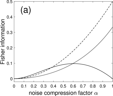
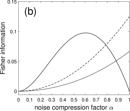
Figure 3: The unitary transformation $\mathsf{U}_{\xi}$ of Eq. (9) is with axis $\vec{n}=[1,0,1]^{\top}/\sqrt{2}$ and phase angle $\xi=\pi/2$. As a function of the compression factor $\alpha$ of the depolarizing noise of Eq. (13), the solid line is the Fisher information $F_{c}^{\rm con}(\xi)=F_{q}^{\rm con}(\xi)$ from Eq. (36) upon measuring the control qubit of the switched quantum channel. The dotted line is the classical Fisher information $F_{c}(\xi)$ of Eq. (42) upon measuring a probe qubit after a one-stage standard cascade as in Fig. 2 with measurement Bloch vector $\vec{\omega}=\vec{e}_{x}$, which is upper-bounded by the quantum Fisher information $F_{q}(\xi)$ of Eq. (43) represented by the dashed line. In (a) the input probe of Eq. (8) is in the pure state $\rho$ with unit Bloch vector $\vec{r}=[1,0,0]^{\top}=\vec{e}_{x}$; in (b) the input probe is in the mixed state $\rho$ with $\vec{r}=[0.5,0,0]^{\top}=\vec{e}_{x}/2$.

When the Bloch vector $\vec{r}$ of the input probe tends to align with the rotation axis $\vec{n}$, Eq. (43) shows that the quantum Fisher information $F_{q}(\xi)$ tends to vanish, and so does any classical Fisher information $F_{c}(\xi)$ attached to any measurement protocol of the probe qubit (even generalized measurements). In this circumstance, measurement of the probe qubit involved in the conventional approach of Eqs. (14) and (41) becomes inefficient to estimate the rotation angle $\xi$. By contrast, as with the measurement probabilities $P^{\rm con}_{\pm}$ of Eq. (26), the Fisher information $F_{c}^{\rm con}(\xi)=F_{q}^{\rm con}(\xi)$ of Eq. (36) for the control qubit of the switched channel, is unaffected by the Bloch vector $\vec{r}$ of the input probe and the axis $\vec{n}$ of the unitary $\mathsf{U}_{\xi}$. As a result, measurement of the control qubit of the switched channel keeps the same estimation efficiency of Eq. (36) irrespective of the situation of the input Bloch vector $\vec{r}$ in relation to the rotation axis $\vec{n}$. The rotation by $\xi$ can even take place on a probe vector $\vec{r}$ parallel to the rotation axis $\vec{n}$, and with $\vec{r}\varparallel\vec{n}$ the control qubit keeps the same estimation efficiency of Eq. (36), while the conventional approach of Eqs. (14) and (41) becomes inoperative.

In a comparable way, when the input probe depolarizes as $\|\vec{r}\,\|\rightarrow 0$, the conventional approach of Eqs. (14) and (41) gradually loses its efficiency for estimating the phase $\xi$, as marked by $F_{q}(\xi)$ in Eq. (43) which vanishes as $\|\vec{r}\,\|\rightarrow 0$. By contrast, the switched channel via its control qubit keeps the same estimation efficiency as in Eq. (36), for any $\|\vec{r}\,\|$. Even at $\|\vec{r}\,\|=0$, when probing with a fully depolarized input probe in the maximally mixed state $\rho=\mathrm{I}_{2}/2$ in Eq. (8), the control qubit of the switched channel remains equally efficient for estimation, while the conventional approach of Eqs. (14) and (41) becomes inoperative.

Figure 3 illustrates in particular the impact of an input probe $\vec{r}$ not orthogonal to the rotation axis $\vec{n}$. At low noise, when the compression factor $\alpha$ is close to $1$ in Fig. 3, direct estimation from the standard cascade is more efficient. Yet, as the level of noise increases when $\alpha$ approaches $0$, the performance of the control qubit of the switched channel quantified by $F_{c}^{\rm con}(\xi)=F_{q}^{\rm con}(\xi)$ of Eq. (36), gradually outperforms both $F_{c}(\xi)$ and then $F_{q}(\xi)$ characterizing the standard cascade of Fig. 2 in conventional estimation. With decreasing $\|\vec{r}\,\|$, when passing from a pure input probe in Fig. 3(a) to a mixed input probe in Fig. 3(b), the performance of the control qubit is unaffected, while the performance of the standard cascade is reduced. This advantage of the control qubit would get more pronounced and would occur earlier (for $\alpha$ closer to $1$) as the input probe $\vec{r}$ approaches the axis $\vec{n}$ or shrinks as $\|\vec{r}\,\|\rightarrow 0$, as explained above. This illustrates the regime of interest for qubit metrology, with an ill-configured input probe $\vec{r}$ or for blind estimation with an unknown axis $\vec{n}$, when the control qubit of the switched channel maintains a uniform unaffected efficiency, while conventional estimation in the standard cascade becomes less efficient.

6.3 Comparison with a two-stage standard cascade

Although the control qubit never directly interacts with the unitary $\mathsf{U}_{\xi}$ under estimation, the switched channel involves two passes of its probe qubit across the unitary $\mathsf{U}_{\xi}$, and it may be compared with a two-stage cascade of a conventional estimation. Equation (42) gives also access to the characterization of a two-stage cascading of the noisy unitary channel involved in Eq. (41), in a standard way with definite causal order. Instead of the one-stage cascading acting as $\vec{r}\mapsto\alpha U_{\xi}\vec{r}$ via Eq. (41), the two-stage cascading acts as $\vec{r}\mapsto\alpha^{2}U_{\xi}^{2}\vec{r}=\alpha^{2}U_{2\xi}\vec{r}$ and is therefore equivalent to a one-stage cascading with the rotation angle $2\xi$ instead of $\xi$ at a noise compression $\alpha^{2}$ instead of $\alpha$. Through these two changes, if the one-stage classical Fisher information of Eq. (42) is denoted $F_{c}(\xi,\alpha)$ then the two-stage cascading is characterized by the Fisher information $F_{c}(2\xi,\alpha^{2})$. The one-stage cascading can provide an estimation of the angle $\xi$ with a minimal root-mean squared (rms) error evolving as $\sim 1/\sqrt{F_{c}(\xi,\alpha)}$; meanwhile the two-stage cascading can provide an estimation of the angle $2\xi$ with a minimal rms error evolving as $\sim 1/\sqrt{F_{c}(2\xi,\alpha^{2})}$, which provides an estimation for $\xi$ with the halved rms error $\sim 1/[2\sqrt{F_{c}(2\xi,\alpha^{2})}]$. For an assessment of a conventional estimation of $\xi$, it is therefore meaningful to confront $F_{c}(\xi,\alpha)$ and $4F_{c}(2\xi,\alpha^{2})$: for a given $\xi$ and a given noise compression $\alpha$, one measurement of the probe qubit after the one-stage cascade delivers about $\xi$ a Fisher information $F_{c}(\xi,\alpha)$, while one measurement of the probe qubit after the two-stage cascade delivers about $\xi$ a Fisher information $4F_{c}(2\xi,\alpha^{2})$. The two-stage cascade amplifies by $2$ the parameter $\xi$ to be estimated, entailing a reduced error, but is also more exposed to the noise, compared with the one-stage cascade. As a result, typically, it can be observed that $4F_{c}(2\xi,\alpha^{2})$ is superior to $F_{c}(\xi,\alpha)$ at small compression with $\alpha$ close to $1$, indicating that the two-stage cascade is more efficient for estimating $\xi$ at low noise level; meanwhile, $F_{c}(\xi,\alpha)$ is superior to $4F_{c}(2\xi,\alpha^{2})$ at large compression with $\alpha$ close to $0$, indicating that the one-stage cascade is more efficient for estimating $\xi$ at high noise level. A similar picture is conveyed by the quantum Fisher information $F_{q}(\xi)$ of Eq. (43), with $F_{q}(\xi,\alpha)=\alpha^{2}(\vec{n}\times\vec{r}\,)^{2}$ for the one-stage cascade, to be confronted with $4F_{q}(2\xi,\alpha^{2})=4\alpha^{4}(\vec{n}\times\vec{r}\,)^{2}$ for the two-stage cascade, with the first which is superior at high noise level (small $\alpha$), and which is used for comparison with the switched channel in Figs. 6–7.

6.4 Phase-averaged performance

The classical Fisher information, $F_{c}(\xi)$ for a standard probe qubit in Eq. (42), or $F_{c}^{\rm con}(\xi)$ for the control qubit of the switched quantum channel in Eq. (36), is dependent on the phase angle $\xi$. This is a common property, often observed for quantum phase estimation in the presence of noise, and implying a performance varying according to the range of the phase $\xi$ to be estimated. A measurement result depending on $\xi$ is necessary to enable estimation of $\xi$ by such measurement. Commonly this entails also a measurement performance depending on $\xi$, and related here to the geometric configuration of the rotated Bloch vector $U_{\xi}\vec{r}$ in $\mathbbm{R}^{3}$. For assessing the performance, it can be meaningful to consider the averaged Fisher information $\overline{F}_{c}=\int_{0}^{2\pi}F_{c}(\xi)d\xi/(2\pi)$ reflecting the average performance for values of $\xi$ uniformly covering the interval $[0,2\pi)$. Especially, for the Fisher information $F_{c}^{\rm con}(\xi)$ in Eq. (36) of the control qubit of the switched channel, the integral over $\xi$ can be worked out explicitly to give

$$\overline{F}_{c}^{\rm con}=1-\frac{\displaystyle\sqrt{3}}{\displaystyle 8}(1-\alpha)\sqrt{(1-\alpha)(3+5\alpha)}-\frac{\displaystyle 1}{\displaystyle 8}\sqrt{(5+6\alpha-3\alpha^{2})(5-2\alpha+5\alpha^{2})}\;.$$ (44)

The average Fisher information in Eq. (44) especially satisfies $\overline{F}_{c}^{\rm con}(\alpha=0)=\overline{F}_{c}^{\rm con}(\alpha=1)=0$ as expected. It is represented and compared in Fig. 4 in conditions where the control qubit of the switched channel offers useful specific capabilities for estimation, with an input probe $\vec{r}$ tending to align with the axis $\vec{n}$ or with a mixed input probe of $\|\vec{r}\,\|<1$.

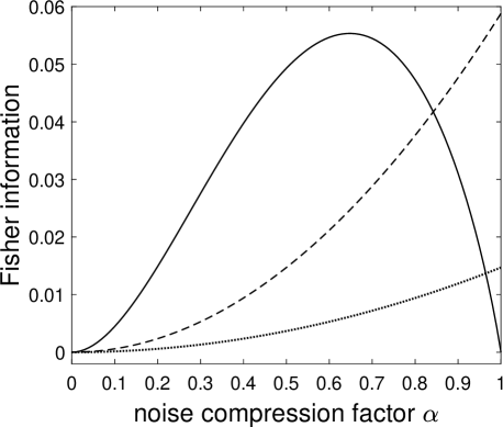
Figure 4: The unitary transformation $\mathsf{U}_{\xi}$ of Eq. (9) is with axis $\vec{n}=[0.8,0,0.2]^{\top}/\sqrt{0.68}$. As a function of the compression factor $\alpha$ of the depolarizing noise of Eq. (13), the solid line is the Fisher information $\overline{F}_{c}^{\rm con}$ of Eq. (44) after averaging over $\xi$ of $F_{c}^{\rm con}(\xi)=F_{q}^{\rm con}(\xi)$ of Eq. (36) for the control qubit of the switched channel. The dashed line is the quantum Fisher information $F_{q}(\xi)$ of Eq. (43) for a one-stage standard cascade as in Fig. 2 and when the input probe in Eq. (8) is in the pure state with unit Bloch vector $\vec{r}=[1,0,0]^{\top}=\vec{e}_{x}$, the dotted line is $F_{q}(\xi)$ of Eq. (43) for the mixed input probe with $\vec{r}=[0.5,0,0]^{\top}=\vec{e}_{x}/2$.

The average Fisher information $\overline{F}_{c}^{\rm con}$, in the conditions of Fig. 4, illustrates that on average over the whole range $[0,2\pi)$ of the phase $\xi$, the control qubit of the switched channel can offer, as the level of noise increases, higher efficiency for estimation compared with the standard cascade of Fig. 2 having to operate with a non-optimized input probe. And this advantage would get more pronounced as the input probe $\vec{r}$ continues to approach the axis $\vec{n}$ or further depolarizes as $\|\vec{r}\,\|\rightarrow 0$.

6.5 Comparison with two qubits in conventional estimation

So far, in the switched channel, measurement of the control qubit, which never directly interacts with the unitary $\mathsf{U}_{\xi}$ under estimation, has been compared with measurement of a qubit involved in a conventional estimation process, in a one-stage or two-stage interaction with the unitary $\mathsf{U}_{\xi}$. This amounts to comparing, for estimation, protocols performing a single measurement on a single qubit, in the switched channel or in a conventional setting. It can also be considered that the switched channel is a two-qubit process, with a control qubit and a probe qubit, so that a comparison with two qubits involved in conventional estimation could offer another meaningful reference. We essentially show below that when estimation has to cope with ill-configured input probes, measurement of the control qubit of the switched channel still displays its useful specificities compared with conventional techniques involving two or more qubits.

If two independent qubits are measured when repeating the conventional estimation of Section 6.2, then the Fisher informations $F_{c}(\xi)$ and $F_{q}(\xi)$ are additive. Especially, from Eq. (43), the quantum Fisher information while measuring two such independent probe qubits is $F_{q}^{(2)}(\xi)=2\alpha^{2}(\vec{n}\times\vec{r}\,)^{2}$. As previously, $F_{q}^{(2)}(\xi)=2\alpha^{2}(\vec{n}\times\vec{r}\,)^{2}$ is maximized when the input probe qubits are prepared in a pure state with $\|\vec{r}\,\|=1$. For an input probe with $\vec{r}$ tending to align with the axis $\vec{n}$ of the unitary $\mathsf{U}_{\xi}$, the conventional estimation measuring two qubits becomes inoperative with $F_{q}^{(2)}(\xi)\rightarrow 0$, while a single measurement of the control qubit of the switched channel keeps the same efficiency as in Eq. (36) or (40), irrespective of the orientation of the input probe. In a similar way, for a depolarized input probe with $\|\vec{r}\,\|\rightarrow 0$, the conventional estimation measuring two qubits becomes inoperative with $F_{q}^{(2)}(\xi)\rightarrow 0$, while a single measurement of the control qubit keeps the same efficiency as in Eq. (36) or (40), unaffected by the depolarization of the probe.

More generally, a two-qubit conventional estimation can use a two-qubit probe prepared in an entangled state $\rho$, and operate according to the various schemes inventoried for instance in [49]. For such two-qubit schemes, the quantum Fisher information $F_{q}^{(2)}(\xi)$, due to its general convexity property [31, 32], is again maximized by a pure input probe state $\rho=\mathinner{|{\psi}\rangle}\mathinner{\langle{\psi}|}$. A direct interaction of two entangled probe qubits in state $\rho$ with the unitary $\mathsf{U}_{\xi}$ under estimation would involve the transformation $\rho\mapsto\mathsf{U}_{\xi}^{(2)}\rho\mathsf{U}_{\xi}^{(2)}\mbox{}^{\dagger}$, with the two-qubit unitary $\mathsf{U}_{\xi}^{(2)}=\mathsf{U}_{\xi}\otimes\mathsf{U}_{\xi}$ for two active qubits in the probe, or $\mathsf{U}_{\xi}^{(2)}=\mathsf{U}_{\xi}\otimes\mathrm{I}_{2}$ for one inactive ancilla qubit in the probe. If the qubit unitary under estimation in Eq. (9) is written $\mathsf{U}_{\xi}=\exp\bigl{(}-i\xi\mathsf{G}\bigr{)}$, with the Hermitian generator $\mathsf{G}=\vec{n}\cdot\vec{\sigma}/2$, then the resulting two-qubit unitary can be put under the form $\mathsf{U}_{\xi}^{(2)}=\exp\bigl{(}-i\xi\mathsf{G}_{2}\bigr{)}$, with the Hermitian generator $\mathsf{G}_{2}=\mathsf{G}\otimes\mathrm{I}_{2}+\mathrm{I}_{2}\otimes\mathsf{G}$ for two active probe qubits, or $\mathsf{G}_{2}=\mathsf{G}\otimes\mathrm{I}_{2}$ for one inactive ancilla qubit in the probe. In the noise-free case, with a pure two-qubit input probe $\rho=\mathinner{|{\psi}\rangle}\mathinner{\langle{\psi}|}$, the quantum Fisher information can be expressed [21, 50] as

$$F_{q}^{(2)}(\xi)=4\Bigl{(}\mathinner{\langle{\psi|\mathsf{G}_{2}^{2}|\psi}\rangle}-\mathinner{\langle{\psi|\mathsf{G}_{2}|\psi}\rangle}^{2}\Bigr{)}=4\mathinner{\langle{\psi|\Delta\mathsf{G}_{2}^{2}|\psi}\rangle}\;,$$ (45)

with the Hermitian variation operator $\Delta\mathsf{G}_{2}=\mathsf{G}_{2}-\mathinner{\langle{\psi|\mathsf{G}_{2}|\psi}\rangle}\mathrm{I}_{2}\otimes\mathrm{I}_{2}$. In the presence of the noise $\mathcal{N}(\cdot)$ affecting the unitary $\mathsf{U}_{\xi}$ as in Fig. 2, the quantum Fisher information is upper bounded [21, 50] as $F_{q}^{(2)}(\xi)\leq 4\mathinner{\langle{\psi|\Delta\mathsf{G}_{2}^{2}|\psi}\rangle}$. As a result, when the state $\mathinner{|{\psi}\rangle}\in\mathcal{H}_{2}\otimes\mathcal{H}_{2}$ of the two-qubit input probe approaches one of the eigenstates of the Hermitian generator $\mathsf{G}_{2}$ (which are the same as the eigenstates of the two-qubit unitary $\mathsf{U}_{\xi}^{(2)}$), the Fisher information $F_{q}^{(2)}(\xi)$ tends to vanish, as its upper limit $4\mathinner{\langle{\psi|\Delta\mathsf{G}_{2}^{2}|\psi}\rangle}$ does. This condition encompasses entangled states $\mathinner{|{\psi}\rangle}$ of the two-qubit input probe. The Hermitian generator $\mathsf{G}=\vec{n}\cdot\vec{\sigma}/2$ has the two eigenvalues $\pm 1/2$ associated with the two eigenstates $\mathinner{|{u_{\pm}}\rangle}$ determined by $\vec{n}$. It results that $\mathsf{U}_{\xi}=\exp\bigl{(}-i\xi\mathsf{G}\bigr{)}$ has the two eigenvalues $\exp(\pm i\xi/2)$ associated with the same two eigenstates $\mathinner{|{u_{\pm}}\rangle}$. As a consequence, $\mathsf{U}_{\xi}^{\otimes 2}$ has the four eigenstates $\bigl{\{}\mathinner{|{u_{+}}\rangle}\otimes\mathinner{|{u_{+}}\rangle},\mathinner{|{u_{-}}\rangle}\otimes\mathinner{|{u_{-}}\rangle},\mathinner{|{u_{+}}\rangle}\otimes\mathinner{|{u_{-}}\rangle},\mathinner{|{u_{-}}\rangle}\otimes\mathinner{|{u_{+}}\rangle}\bigr{\}}$, associated respectively with the four eigenvalues $\bigl{\{}e^{i\xi},e^{-i\xi},+1,+1\bigr{\}}$. Because of the degeneracy of the eigenvalue $+1$, the two states $\mathinner{|{w_{\pm}}\rangle}=\bigl{(}\mathinner{|{u_{+}}\rangle}\otimes\mathinner{|{u_{-}}\rangle}\pm\mathinner{|{u_{-}}\rangle}\otimes\mathinner{|{u_{+}}\rangle}\bigr{)}/\sqrt{2}$ are two eigenstates of $\mathsf{U}_{\xi}^{\otimes 2}$ with eigenvalue $+1$, and are two entangled states of the two qubits. Any linear combination of $\mathinner{|{w_{+}}\rangle}$ and $\mathinner{|{w_{-}}\rangle}$ will also in general represent an entangled eigenstate of $\mathsf{U}_{\xi}^{\otimes 2}$ with the eigenvalue $+1$. This represents a two-dimensional subspace of $\mathcal{H}_{2}^{\otimes 2}$. When such two-qubit entangled states are used to probe the unitary $\mathsf{U}_{\xi}$ (or when the two-qubit state tends to align with such subspace), they also become inoperative for conventional estimation. These configurations stand as the two-qubit analogue of the one-qubit probe tending to align with the axis $\vec{n}$ of the unitary $\mathsf{U}_{\xi}$. So with such two-qubit input probes tending to align with $\mathsf{U}_{\xi}$ in this sense, the conventional estimation measuring two qubits becomes inoperative with $F_{q}^{(2)}(\xi)\rightarrow 0$, while again a single measurement of the control qubit of the switched channel keeps the same efficiency as in Eq. (36) or (40), irrespective of the configuration of the input probe.

In addition, a fully depolarized two-qubit input probe $\rho=\mathrm{I}_{2}\otimes\mathrm{I}_{2}/4$ gives the interaction $\mathsf{U}_{\xi}^{(2)}\rho\mathsf{U}_{\xi}^{(2)}\mbox{}^{\dagger}=\mathrm{I}_{2}\otimes\mathrm{I}_{2}/4$ leaving the probe invariant and insensitive to the phase $\xi$. The corresponding Fisher information is $F_{q}^{(2)}(\xi)=0$, and the conventional estimation measuring two qubits becomes inoperative with such a depolarized input probe, while again a single measurement of the control qubit of the switched channel keeps the same efficiency as in Eq. (36) or (40), unaffected by the depolarization of the probe.

Two-qubit conventional estimation can also be considered with only one depolarized qubit in the two-qubit probe. The switched channel uses a coherent control qubit that does not directly interact with the unitary $\mathsf{U}_{\xi}$ but gets entangled to the probe qubit interacting with $\mathsf{U}_{\xi}$. In this respect, we can consider conventional estimation with an input qubit pair of an active qubit and an inactive qubit, prepared in an arbitrary entangled (possibly optimized in some way) state. Then, before it can interact with the unitary $\mathsf{U}_{\xi}$ to probe it, we consider that the active qubit gets (or tends to be) completely depolarized, by some noise affecting the preparation, and so as to place it in the situation of the completely depolarized probe qubit of the switched channel; meanwhile the entangled inactive qubit remains untouched and unaffected by the depolarization. Then, in this condition also, the two-qubit probe becomes completely inoperative for conventional estimation. This follows directly by the action of $\mathsf{U}_{\xi}$ on a fully depolarized qubit, leaving its state invariant and insensitive to the phase $\xi$; or also by explicit evaluation of the quantum Fisher information obtained for instance from [32] for this two-qubit estimation scheme. Meanwhile, as indicated, a single measurement of the control qubit of the switched channel remains operative for estimation when probing with a fully depolarized probe qubit.

The above features related to conventional estimation carry over with additional $\xi$-independent unitaries intervening in the processing of the two qubits, and also with conventional techniques employing and measuring more than two qubits, active or inactive, for multiple probing of the unitary $\mathsf{U}_{\xi}$. With a multiple-qubit input probe tending to align with the unitary or approaching a fully depolarized preparation, measurement of the multiple qubits becomes inoperative in conventional estimation of $\xi$, while a single measurement of the control qubit of the switched channel keeps the same estimation efficiency as in Eq. (36) or (40).

This of course does not alter the fact that conventional estimation, especially with multiple qubits, remains useful in its own right, especially in controlled conditions where it can be optimized. This, in particular, usually requires the knowledge of the axis $\vec{n}$ of the unitary $\mathsf{U}_{\xi}$ under estimation, with well controlled probing inputs, and conditions exist, especially in the presence of noise, where the optimal configurations are also dependent on the unknown phase itself and therefore inaccessible in practice [20, 34]. As a complement, in other distinct yet meaningful conditions that we report here, the switched channel can bring additional capabilities for estimation, via the novel approach of switched indefinite causal order shown here applicable for qubit phase estimation.

6.6 For the probe qubit of the switched channel

In the switched quantum channel, after measurement of the control qubit, the probe qubit gets placed in the conditional state $\rho_{\pm}^{\rm post}$ of Eqs. (28)–(29) which in general also depends on the phase $\xi$. Measuring $\rho_{\pm}^{\rm post}$ can therefore provide useful additional information to estimate $\xi$. For an assessment, it is possible to evaluate the Fisher information, classical or quantum, in the state $\rho_{\pm}^{\rm post}$ about $\xi$. For a viewpoint not attached to a specific measurement protocol of $\rho_{\pm}^{\rm post}$, one can turn to the quantum Fisher information of Eq. (33) applied to the Bloch vector $\vec{r}_{\pm}^{\rm\,post}(\xi)\equiv\vec{r}_{\xi}$ from Eq. (29). For this purpose, $\vec{r}_{\pm}^{\rm\,post}(\xi)$ in Eq. (29) especially involves a quadratic function of the matrix $U_{\xi}$, and from Eq. (29) it is feasible to analytically compute the derivative $\partial_{\xi}\vec{r}_{\pm}^{\rm\,post}(\xi)$, noting that for two $\xi$-dependent matrices $A_{\xi}$ and $B_{\xi}$ one has the derivative $\partial_{\xi}(A_{\xi}B_{\xi})=(\partial_{\xi}A_{\xi})B_{\xi}+A_{\xi}(\partial_{\xi}B_{\xi})$. It is in this way feasible to obtain an analytical expression for the quantum Fisher information $F_{q}^{\rm swi}(\xi)$ for the probe qubit of the switched channel, from Eq. (33), when $\vec{r}_{\xi}\equiv\vec{r}_{\pm}^{\rm\,post}(\xi)$ from Eq. (29); but this expression is rather bulky and we will not write it here.

It is observed with the switched channel that in general the Fisher information $F_{q}^{\rm swi}(\xi)$ of the probe states $\rho_{+}^{\rm post}$ and $\rho_{-}^{\rm post}$ does depend on both $\xi$ and $\vec{n}$, and also on the input probe $\vec{r}$. As the input probe depolarizes, with $\|\vec{r}\,\|\rightarrow 0$, Eq. (29) shows that $\vec{r}_{\pm}^{\rm\,post}(\xi)$ both vanish and so does the corresponding Fisher information $F_{q}^{\rm swi}(\xi)$. Therefore, in contrary to the control qubit, the probe qubit of the switched channel becomes inoperative for estimation with a fully depolarized input probe. However, in similarity with the control qubit, the estimation efficiency of the probe qubit assessed by $F_{q}^{\rm swi}(\xi)$ does not uniformly vanish for an input probe $\vec{r}$ parallel to the rotation axis $\vec{n}$. This is a specific property of the switched channel for estimation, accessible both by measuring either the control qubit or the probe qubit, enabling to perform estimation of the phase angle $\xi$ even with an input probe $\vec{r}$ parallel to the axis $\vec{n}$ of the unitary $\mathsf{U}_{\xi}$. This property is not present in conventional estimation, as addressed in Sections 6.2 and 6.3, even when repeated on multiple qubits as in Section 6.5. This specific property of the probe qubit of the switched channel is illustrated in Fig. 5, showing a nonzero Fisher information $F_{q}^{\rm swi}(\xi)$ with an input probe $\vec{r}$ parallel to the axis $\vec{n}$ of the unitary $\mathsf{U}_{\xi}$, while in such condition the Fisher information of conventional estimation is expected to be zero, as addressed in Sections 6.2, 6.3 and 6.5.

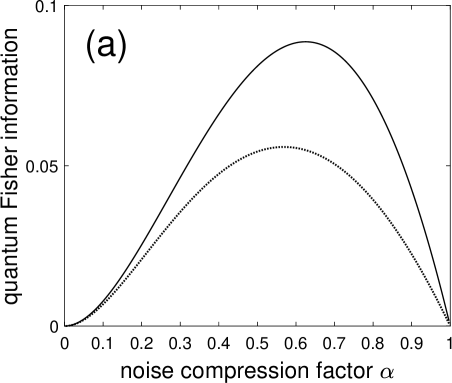
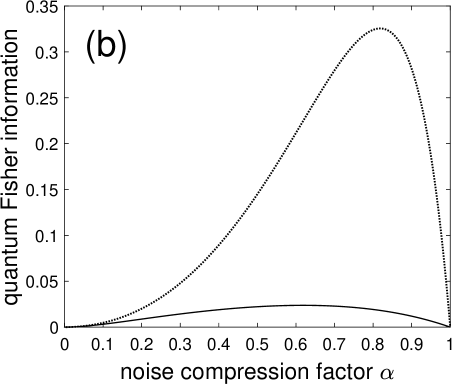
Figure 5: The unitary transformation $\mathsf{U}_{\xi}$ of Eq. (9) is with axis $\vec{n}=[1,0,0]^{\top}=\vec{e}_{x}$, the input probe in Eq. (8) is in the pure state with unit Bloch vector $\vec{r}=\vec{n}$, and in abscissa is the compression factor $\alpha$ of the depolarizing noise of Eq. (13). For the probe qubit of the switched channel, the quantum Fisher information $F_{q}^{\rm swi}(\xi)$ from Eq. (33) associated with the state $\rho_{+}^{\rm post}$ (solid line), and $\rho_{-}^{\rm post}$ (dotted line). The phase angle is $\xi=\pi/2$ in (a), and $\xi=\pi/4$ in (b).

Figure 5 illustrates specific conditions, when $\vec{r}\varparallel\vec{n}$, where the probe qubit of the switched channel can offer an advantage over conventional estimation. Beyond, the performance of both approaches to estimation will vary much with the conditions, the configuration of the input probe $\vec{r}$, pure or mixed, in relation to the axis $\vec{n}$, the range of the parameter $\xi$, the level of noise, the number of passes or repetitions for conventional techniques. For further quantitative illustration, the performance for estimation upon measuring the probe qubit of the switched channel is compared below with conventional estimation upon measuring also a single qubit, as in Section 6.2 and 6.3, especially to show other conditions where the switched channel can bring useful contribution.

For a unit input probe $\vec{r}$ nonparallel and nonorthogonal to the rotation axis $\vec{n}$, Fig. 6(a) shows that the quantum Fisher information $F_{q}^{\rm swi}(\xi)$ associated with the probe state $\rho_{+}^{\rm post}$ can surpass the quantum Fisher information $F_{q}(\xi)$ associated with a one-stage and a two-stage standard cascade from Fig. 2. This occurs for some range of the phase $\xi$ around $\pi/2$ in Fig. 6(a), while in the range of $\xi$ around $\pi/4$ Fig. 6(b) shows that it is $F_{q}^{\rm swi}(\xi)$ of $\rho_{-}^{\rm post}$ that can dominate. The efficiency quantified by the Fisher information $F_{q}^{\rm swi}(\xi)$ in Fig. 6, of measuring for estimation the state $\rho_{+}^{\rm post}$ or the state $\rho_{-}^{\rm post}$, is determined by the geometric configuration of their respective Bloch vector $\vec{r}_{+}^{\rm\,post}$ or $\vec{r}_{-}^{\rm\,post}$ in $\mathbbm{R}^{3}$, as it results from Eq. (29) to act in Eq. (33). As observed in Fig. 6, depending on the conditions, $\vec{r}_{+}^{\rm\,post}$ and $\vec{r}_{-}^{\rm\,post}$ change according to Eq. (29), and consequently $\rho_{+}^{\rm post}$ or $\rho_{-}^{\rm post}$ present more efficient configurations for estimation. Also, the advantage of the switched channel observed in Fig. 6 would get more pronounced as the input probe $\vec{r}$ tends to align with the axis $\vec{n}$.

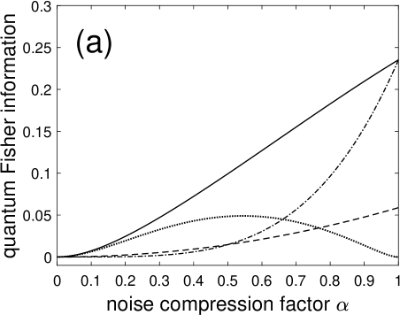
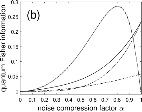
Figure 6: As in Fig. 4, the unitary transformation $\mathsf{U}_{\xi}$ of Eq. (9) is with axis $\vec{n}=[0.8,0,0.2]^{\top}/\sqrt{0.68}$, the input probe in Eq. (8) is in the pure state with unit Bloch vector $\vec{r}=[1,0,0]^{\top}=\vec{e}_{x}$, and in abscissa is the compression factor $\alpha$ of the depolarizing noise of Eq. (13). For the probe qubit of the switched channel, the quantum Fisher information $F_{q}^{\rm swi}(\xi)$ from Eq. (33) associated with the state $\rho_{+}^{\rm post}$ (solid line), and $\rho_{-}^{\rm post}$ (dotted line). From Eq. (43), the dashed line is the quantum Fisher information $F_{q}(\xi,\alpha)=\alpha^{2}(\vec{n}\times\vec{r}\,)^{2}$ for a one-stage standard cascade as in Fig. 2, while the dashed-dotted line is $4F_{q}(2\xi,\alpha^{2})=4\alpha^{4}(\vec{n}\times\vec{r}\,)^{2}$ for a two-stage standard cascade. The phase angle is $\xi=\pi/2$ in (a), and $\xi=\pi/4$ in (b).

A comparable picture is obtained when the quantum Fisher information $F_{q}^{\rm swi}(\xi)$ from the probe state $\rho_{\pm}^{\rm post}$ is averaged as $\overline{F}_{q}\mbox{}\!^{\rm swi}$ over the phase $\xi$ uniform in $[0,2\pi)$, as illustrated in Fig. 7.

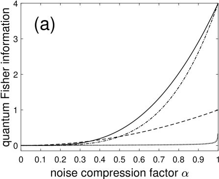
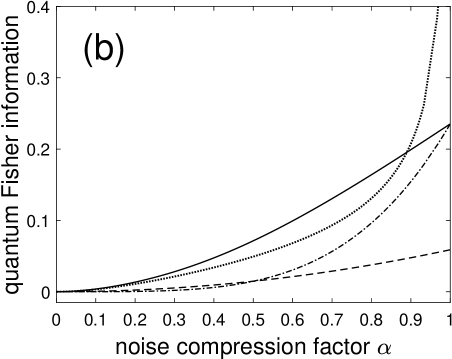
Figure 7: The input probe in Eq. (8) is in the pure state with unit Bloch vector $\vec{r}=[1,0,0]^{\top}=\vec{e}_{x}$, and in abscissa is the compression factor $\alpha$ of the depolarizing noise of Eq. (13). For the probe qubit of the switched channel, the quantum Fisher information $F_{q}^{\rm swi}(\xi)$ from Eq. (33) associated with the state $\rho_{+}^{\rm post}$ (solid line), and $\rho_{-}^{\rm post}$ (dotted line), after it has been averaged over the phase $\xi$ uniform in $[0,2\pi)$. From Eq. (43), the dashed line is the quantum Fisher information $F_{q}(\xi,\alpha)=\alpha^{2}(\vec{n}\times\vec{r}\,)^{2}$ for a one-stage standard cascade as in Fig. 2, while the dashed-dotted line is $4F_{q}(2\xi,\alpha^{2})=4\alpha^{4}(\vec{n}\times\vec{r}\,)^{2}$ for a two-stage standard cascade. The unitary transformation $\mathsf{U}_{\xi}$ of Eq. (9) is with axis $\vec{n}=[0,0,1]^{\top}=\vec{e}_{z}$ in (a), and $\vec{n}=[0.8,0,0.2]^{\top}/\sqrt{0.68}$ in (b).

In Fig. 7 it can be observed that the phase-averaged quantum Fisher information $\overline{F}_{q}\mbox{}\!^{\rm swi}$ of the probe qubit from the switched channel, can still surpass the Fisher information from the standard cascade of Fig. 2, either one-stage as $F_{q}(\xi,\alpha)=\alpha^{2}(\vec{n}\times\vec{r}\,)^{2}$ or two-stage as $4F_{q}(2\xi,\alpha^{2})=4\alpha^{4}(\vec{n}\times\vec{r}\,)^{2}$. This advantage is even observed with an optimal unit input probe $\vec{r}$ orthogonal to the axis $\vec{n}$ as shown in Fig. 7(a), and it gets in some respect more pronounced as $\vec{r}$ approaches $\vec{n}$ as illustrated in Fig. 7(b).

When characterizing the estimation performance in the switched channel by means of the quantum Fisher information $F_{q}^{\rm swi}(\xi)$ upon measuring the probe qubit state $\rho_{\pm}^{\rm post}$ as done in Figs. 5–7, we have to keep in mind that $\rho_{\pm}^{\rm post}$ represent two conditional states occurring according to the probabilities $P^{\rm con}_{\pm}$ of Eq. (26). So the corresponding performance assessed by $F_{q}^{\rm swi}(\xi)$ attached to $\rho_{+}^{\rm post}$ or $\rho_{-}^{\rm post}$ applies also conditionally, with the probabilistic weights $P^{\rm con}_{\pm}$. At the favorable setting $p_{c}=1/2$ where we are, it follows from Eq. (26) that $P^{\rm con}_{+}$ always stays above $P^{\rm con}_{-}$ for any $\alpha\in[0,1]$, and $P^{\rm con}_{+}$ goes to $1$ at low noise when $\alpha\rightarrow 1$ while $P^{\rm con}_{+}$ approaches $P^{\rm con}_{-}$ but stays above it at large noise when $\alpha\rightarrow 0$. So the post-measurement state $\rho_{+}^{\rm post}$ for the probe qubit is always more probable, and almost certain at low noise when $\alpha\rightarrow 1$. The evolutions of $F_{q}^{\rm swi}(\xi)$ for $\rho_{\pm}^{\rm post}$, as exemplified in Figs. 5–7, although they have to be probabilistically weighted for their interpretation, nevertheless reveal useful capabilities accessible by measuring the probe qubit of the switched channel for phase estimation.

For estimating the phase $\xi$ with the switched quantum channel, if one resorts to measuring the probe qubit as well as the control qubit, then an a-priori more efficient approach would be to envisage a joint measurement of the qubit pair in the entangled state $\mathcal{S}(\rho\otimes\rho_{c})$ of Eq. (15). The measurement results will generally be governed by a $\xi$-dependent probability distribution. From there, an estimator, such as the maximum likelihood estimator, could be conceived for $\xi$, along with the associated Fisher information for an assessment of the performance. This approach is made possible based on the complete characterization of the joint state $\mathcal{S}(\rho\otimes\rho_{c})$ worked out in Section 4. A joint measurement of the two qubits, control and probe, of the switched channel could naturally be compared with conventional estimation schemes measuring two qubits, active or ancilla, as in [49] and in Section 6.5 here. Such joint estimation involving the two qubits of the switched channel is however more complicated to characterize analytically, and depends on the choice of the joint measurement involved. We leave it as an open perspective, to come after the present work that has demonstrated potentialities of the switched quantum channel with indefinite causal order for contributing to parameter estimation and metrology.

7 Discussion and conclusion

In the present work we have considered a noisy unitary channel according to Fig. 2, when two copies of this channel are interconnected in indefinite causal order by a quantum switch process as in Fig. 1. An original contribution of the present work is, for a generic qubit unitary operator $\mathsf{U}_{\xi}$ affected by a depolarizing noise, the characterization of the transformation realized by the switched quantum channel of Fig. 1 and worked out in Section 4. This characterization lies essentially in the quantum operation $\mathcal{S}(\rho\otimes\rho_{c})$ of Eq. (15) acting on the joint state of the probe-control qubit pair. We have fully characterized this action in Bloch representation via the superoperator $\mathcal{S}_{00}(\rho)$ of Eq. (16), and – for the most substantial part – the superoperator $\mathcal{S}_{01}(\rho)$ of Eq. (17) determined by $\mathcal{S}_{01}(\mathrm{I}_{2})$ in Eq. (21) and $\mathcal{S}_{01}(\vec{r}\cdot\vec{\sigma})$ in Eq. (22). This theoretical characterization of Section 4 then enabled us in Sections 5 and 6 to realize an analysis of the switched channel and its performance for a task of phase estimation on the unitary operator $\mathsf{U}_{\xi}$ with depolarizing noise. A comparison has also been made with conventional techniques of estimation where the noisy unitary is directly probed in a one-stage or two-stage cascade with definite order, or several uses of them with two or more qubits. Especially, the analysis has demonstrated three specific properties of the switched channel, meaningful for estimation and not present with conventional techniques.

The first significant property is that the control qubit of the switched channel, although it never directly interacts with the unitary $\mathsf{U}_{\xi}$, can nevertheless be measured for the phase estimation on $\mathsf{U}_{\xi}$; and it can be measured alone, while discarding the probe qubit that interacts with the unitary $\mathsf{U}_{\xi}$ under estimation. This possibility results from the specific entanglement realized between the control and probe qubits by the interaction of the quantum switch process characterized in Section 4. This control-probe entangled qubit pair in the switched channel presents some similarity with conventional strategies as for instance analyzed in [49], where active probing qubits can receive assistance for estimation from passive ancilla qubits not directly interacting with the process under estimation. However, there exists an essential difference in that in such conventional estimation strategies, the inactive ancilla qubits must be jointly measured with the active probing qubits to be of some use, and the ancilla qubits measured alone are inoperative for estimation. By contrast, in the switched channel here, the control qubit alone can be measured for estimation.

The second significant property is that the control qubit of the switched channel maintains a uniform efficiency for estimation, even when the input probe qubit of switched channel tends to align and becomes parallel with the axis $\vec{n}$ of the unitary $\mathsf{U}_{\xi}$. In a standard interaction with the qubit unitary $\mathsf{U}_{\xi}$ as in Eq. (41), rotation of a probe qubit $\vec{r}$ parallel to the rotation axis $\vec{n}$ issues no physical effect or information enabling any access to the rotation angle $\xi$. This mechanism of rotating an isolated qubit does not hold with the switched quantum channel, which rather acts on a probe-control entangled qubit pair in the specific way characterized in Section 4 enabling estimation even with an input probe with $\vec{r}\varparallel\vec{n}$.

The third significant property is that the control qubit of the switched channel also maintains a uniform efficiency for estimation, even when the input probe qubit of switched channel tends to depolarize or even becomes completely depolarized when $\|\vec{r}\,\|=0$. Conventional techniques based on the qubit interaction $\rho\mapsto\mathsf{U}_{\xi}\rho\mathsf{U}_{\xi}^{\dagger}$ have no effect on the completely depolarized input probe $\rho=\mathrm{I}_{2}/2$, which remains invariant and insensitive to the phase $\xi$ and thus inoperative for estimating $\xi$. By contrast, the specific interaction in the switched channel with indefinite order we characterized in Section 4 makes it possible to use a fully depolarized input probe for estimation.

Conventional estimation techniques, as addressed in Sections 6.2, 6.3 and 6.5, although useful in their own right, do not share these properties of the switched channel, and they become gradually inoperative when the input probe tends to align with the unitary $\mathsf{U}_{\xi}$ under estimation or progressively depolarizes. These three properties relevant to estimation are essentially contributed by the control qubit of the switched channel, and they manifest specific and unusual capabilities for quantum information processing observable in channels with coherent control of indefinite causal order, as also observed for instance in [8]. We have also analyzed in Section 6.6 the measurement of the probe qubit of the switched channel and showed it can add useful capabilities for phase estimation. These specific and unusual properties of the switched channel for estimation, and specially the capabilities of its control qubit, stem from the specific interaction entangling the two qubits in the joint state $\mathcal{S}(\rho\otimes\rho_{c})$ of Eq. (15) characterized in Section 4. An essential ingredient is the qubit superoperator $\mathcal{S}_{01}(\cdot)$ of Eqs. (5) and (17), which is a specific interaction term following from the coherent superposition of causal orders implemented by the switch process according to Eqs. (1)–(2). This interaction term $\mathcal{S}_{01}(\cdot)$ acts in the joint state $\mathcal{S}(\rho\otimes\rho_{c})$ of Eq. (15) only when there exists an effective coherent superposition of orders, at $p_{c}\not=0,1$ for the control qubit. The switch process of Eqs. (1)–(2) then mixes two elementary channels having Kraus operators that do not commute, as explained at the end of Section 4. Their combinations in $\mathcal{S}_{01}(\cdot)$ of Eqs. (5) and (17) superpose various paths across the operators determining the transmission by the composite switched channel. In particular, these combinations of paths in Eqs. (5) and (17) lead for the interaction term to $\mathcal{S}_{01}(\mathrm{I}_{2})\not=\mathrm{I}_{2}$, as expressed by Eq. (21), which has a direct impact for the transmission of the fully depolarized input probe $\rho=\mathrm{I}_{2}/2$, and also more generally of the generic input probe $\rho$ of Eq. (8). With the generic input probe of Eq. (8), this specific interaction in the switched channel via the superoperator $\mathcal{S}_{01}(\rho)$ of Eq. (17), leads to a control qubit in the state $\rho^{\rm con}_{\xi}$ of Eqs. (37)–(38), which is unaffected by $\vec{r}$ but sensitive to $\xi$, essentially by way of $\operatorname{tr}[\mathcal{S}_{01}(\rho)]=\operatorname{tr}[\mathcal{S}_{01}(\mathrm{I}_{2})/2]=Q_{\xi}(\alpha)\not=1$, for any $\vec{r}$. As a result, measurement of the control qubit in the state $\rho^{\rm con}_{\xi}$, as governed by the probabilities $P^{\rm con}_{\pm}$ of Eqs. (25)–(26), is unaffected by $\vec{r}$, but remains sensitive to $\xi$, even when $\vec{r}\varparallel\vec{n}$ and $\|\vec{r}\,\|=0$, affording estimation capabilities in these conditions.

The characterization of $\mathcal{S}(\rho\otimes\rho_{c})$ carried out in Section 4 with the important reference formed by the depolarizing noise, could be extended to other qubit noise models. Arbitrary Pauli noises could be incorporated with three distinct probabilities $p_{x}$, $p_{y}$, $p_{z}$ for the three Pauli operators in Eq. (12) instead of the common probability $p/3$. Then the derivation of Section 4 could proceed in a similar way, except at the stage where relations like Eqs. (A-4) and (A-9) would have to be incorporated into Eq. (17) in accordance with the specific probabilistic weights $p_{x}$, $p_{y}$ or $p_{z}$; and similarly for Eq. (A-19) and Eqs. (A-28)–(A-30). This would lead to more bulky expressions, but useful capabilities of the switched channel can be expected to be preserved. We have explicitly tested a bit-flip noise and a phase-flip noise, and verified that both preserve the essential capabilities of the switched channel with indefinite causal order useful to estimation, yet with added variability in the detailed performance especially depending on the angle between the privileged axis of the noise and the orientation $\vec{n}$ of the unitary $\mathsf{U}_{\xi}$.

This robustness with various noise models is also an interesting feature to robustly preserve the capabilities for estimation from the switched channel in concrete physical implementations. Also, as observed in Section 6, a defective preparation (pure or mixed) of the input probe qubit will have no effect on the efficiency for estimation from the control qubit. In addition, as observed in Section 5, an indefinite superposition of causal orders robustly takes place for any $p_{c}\in(0,1)$ in the preparation of the control qubit $\mathinner{|{\psi_{c}}\rangle}=\sqrt{p_{c}}\mathinner{|{0}\rangle}+\sqrt{1-p_{c}}\mathinner{|{1}\rangle}$. From these properties, it can be expected that the capabilities useful to estimation of the switched channel will be robustly preserved in physical implementations with experimental imperfections.

Previous works on quantum switched channels with indefinite order concentrated first on communication of information [8, 9, 10, 11], and more recently on parameter estimation yet in significantly distinct processes and conditions [14, 15, 16]. By comparison, specificities of our study are that it considers a qubit system, experiencing a generic qubit unitary operator $\mathsf{U}_{\xi}$, characterized by an unknown parameter $\xi$ to be estimated. Parameter estimation on a qubit unitary process represents an important reference task for quantum metrology, which is investigated here for the first time in quantum switched channels with indefinite order. In addition, in the estimation task, the realistic condition where noise is present is taken into account as a significant specificity.

The capability of the switched channel for estimation with a fully depolarized input probe is reminiscent of the situation of the quantum communication channel analyzed for instance in [8] as evoked in the Introduction. In [8], an isolated communication channel is by itself fully depolarizing and unable to transmit any useful information, with a zero Holevo information or information capacity. When duplicated and inserted in a quantum switch process as in Fig. 1 with indefinite causal order, it gives rise to a quantum channel with nonzero information capacity, enabling effective transmission of information. We observe a comparable behavior here, for an estimation task rather than a communication task, assessed by the Fisher information instead of the information capacity. The effect in [8] is observed with a coherent control to superpose two depolarizing channels in indefinite causal order. In a recent study [51] related to [8], a comparable effect is observed with no indefinite causal order, but instead with a coherent control to determine which of the two depolarizing channels is traversed. These are two distinct phenomena, which can be observed separately as in [8] and in [51], and which are further discussed in [52, 11]. The effects for estimation in our study occur in the presence of coherent control of indefinite causal order, as in [8]. Examining if the effects we observe would occur or not in the setting of [51] having coherent control but no indefinite causal order, could possibly help to disentangle the respective roles of coherent control and indefinite order. Such an extension would contribute to the exploration of the properties and capabilities of coherent quantum superposition of processing channels, with the structure of either [8] or [51].

The specific capabilities uncovered here for estimation will be practically accessible at the cost of physically implementing the quantum switch process. In this respect, techniques have been proposed that are particularly appealing for photonic implementations, as in [3] for instance, with an interferometric setup, by combining a spatial mode of a photon for the control with its polarization for the probe. Employing such setups for estimation could render practically accessible the useful properties of the switched process in photon metrology and interferometry, where qubit phase estimation is an essential operation, at the root of many applications such as high-sensitivity and high-precision measurements, atomic clocks, frequency standards [17, 19, 23, 24, 25, 26]. In particular, if the probe and control qubits can physically be made sufficiently distant when the probe interacts with the unitary, specially interesting properties could follow.

In this way, the present study contributes to the identification and analysis of the properties and capabilities of switched quantum channels with indefinite causal order for quantum signal and information processing, along with new possibilities useful to quantum estimation and qubit metrology.

Appendix A

In this Appendix we work out the Bloch representation for $\mathcal{S}_{01}(\mathrm{I}_{2})$ and $\mathcal{S}_{01}(\vec{r}\cdot\vec{\sigma})$ characterizing the superoperator $\mathcal{S}_{01}(\rho)$ of Eq. (17).

$\bullet$ For $\mathcal{S}_{01}(\mathrm{I}_{2})\,$:

By unitarity of $\mathsf{U}_{\xi}$, in Eq. (18) one has $\mathcal{W}_{0}(\mathrm{I}_{2})=\mathrm{I}_{2}$. In Eq. (19) one has $\mathcal{W}_{\ell}(\mathrm{I}_{2})=\sigma_{\ell}\mathsf{U}_{\xi}\sigma_{\ell}\mathsf{U}_{\xi}^{\dagger}$. Terms comparable to $\sigma_{\ell}\mathsf{U}_{\xi}$ can be evaluated via Eq. (9) and the standard behavior of products of Pauli operators. One obtains, for $\mathcal{W}_{x}(\mathrm{I}_{2})$ for instance,

$$\sigma_{x}\mathsf{U}_{\xi}=\cos(\xi/2)\sigma_{x}+\sin(\xi/2)(-n_{z}\sigma_{y}+n_{y}\sigma_{z}-in_{x}\mathrm{I}_{2})\;,$$ (A-1)

and also

$$\sigma_{x}\mathsf{U}_{\xi}^{\dagger}=\cos(\xi/2)\sigma_{x}+\sin(\xi/2)(n_{z}\sigma_{y}-n_{y}\sigma_{z}+in_{x}\mathrm{I}_{2})\;,$$ (A-2)

which gives

$$\sigma_{x}\mathsf{U}_{\xi}\sigma_{x}\mathsf{U}_{\xi}^{\dagger}=\left(1-2\sin^{2}\Bigl{(}\frac{\xi}{2}\Bigr{)}(1-n_{x}^{2})\right)\mathrm{I}_{2}+i2\sin\Bigl{(}\frac{\xi}{2}\Bigr{)}\left(\cos\Bigl{(}\frac{\xi}{2}\Bigr{)}\begin{bmatrix}0\\ n_{y}\\ n_{z}\end{bmatrix}+\sin\Bigl{(}\frac{\xi}{2}\Bigr{)}n_{x}\begin{bmatrix}0\\ -n_{z}\\ n_{y}\end{bmatrix}\right)\cdot\vec{\sigma}\;,$$ (A-3)

resulting in

$$\bigl{(}\mathcal{W}_{x}+\mathcal{W}_{x}^{\dagger}\bigr{)}(\mathrm{I}_{2})=2\bigl{[}1-2\sin^{2}(\xi/2)(1-n_{x}^{2})\bigr{]}\mathrm{I}_{2}\;.$$ (A-4)

Similar relations can be obtained for $\mathcal{W}_{y}(\mathrm{I}_{2})$ and $\mathcal{W}_{z}(\mathrm{I}_{2})$ and their adjoints, and due to the isotropic action of the depolarizing noise in $\mathbbm{R}^{3}$, they add up uniformly in Eq. (17) so as to give

$$\sum_{\ell=x,y,z}\bigl{(}\mathcal{W}_{\ell}+\mathcal{W}_{\ell}^{\dagger}\bigr{)}(\mathrm{I}_{2})=2\bigl{[}3-4\sin^{2}(\xi/2)\bigr{]}\mathrm{I}_{2}\;.$$ (A-5)

For $\mathcal{W}_{\ell\ell^{\prime}}(\mathrm{I}_{2})$ in Eq. (20) one has for instance $\mathcal{W}_{xy}(\mathrm{I}_{2})=\sigma_{x}\mathsf{U}_{\xi}\sigma_{y}\sigma_{x}\mathsf{U}_{\xi}^{\dagger}\sigma_{y}=-i\sigma_{x}\mathsf{U}_{\xi}\sigma_{z}\mathsf{U}_{\xi}^{\dagger}\sigma_{y}$. Via the circular permutation behavior among Pauli operators and their products, relations analogous to Eqs. (A-1)–(A-2) readily follow, as for instance

$$\sigma_{z}\mathsf{U}_{\xi}^{\dagger}=\cos(\xi/2)\sigma_{z}+\sin(\xi/2)(n_{y}\sigma_{x}-n_{x}\sigma_{y}+in_{z}\mathrm{I}_{2})\;.$$ (A-6)

From Eqs. (A-1) and (A-6) one has

$$\sigma_{x}\mathsf{U}_{\xi}\sigma_{z}\mathsf{U}_{\xi}^{\dagger} = -i\cos^{2}(\xi/2)\sigma_{y}+2\cos(\xi/2)\sin(\xi/2)(n_{y}\mathrm{I}_{2}-in_{x}\sigma_{z})$$

$$+ \sin^{2}(\xi/2)\bigl{[}2n_{x}n_{z}\mathrm{I}_{2}+i(1-2n_{z}^{2})\sigma_{y}+i2n_{y}n_{z}\sigma_{z}\bigr{]}\;,$$ (A-7)

and by right-multiplying by $-i\sigma_{y}$ one obtains

$$\mathcal{W}_{xy}(\mathrm{I}_{2}) = \bigl{[}-\cos^{2}(\xi/2)+\sin^{2}(\xi/2)(1-2n_{z}^{2})\bigr{]}\mathrm{I}_{2}$$

$$+ i2\bigl{[}\cos(\xi/2)\sin(\xi/2)(n_{x}\sigma_{x}-n_{y}\sigma_{y})-\sin^{2}(\xi/2)n_{z}(n_{y}\sigma_{x}+n_{x}\sigma_{y})\bigr{]}\;,$$ (A-8)

yielding

$$\bigl{(}\mathcal{W}_{xy}+\mathcal{W}_{xy}^{\dagger}\bigr{)}(\mathrm{I}_{2})=2\bigl{[}-1+2\sin^{2}(\xi/2)(1-n_{z}^{2})\bigr{]}\mathrm{I}_{2}\;.$$ (A-9)

Two other relations similar to Eq. (A-9) can be obtained, which again, due to the isotropic action of the depolarizing noise in $\mathbbm{R}^{3}$, add up uniformly in Eq. (17) to provide

$$\bigl{[}\bigl{(}\mathcal{W}_{xy}+\mathcal{W}_{xy}^{\dagger}\bigr{)}+\bigl{(}\mathcal{W}_{yz}+\mathcal{W}_{yz}^{\dagger}\bigr{)}+\bigl{(}\mathcal{W}_{zx}+\mathcal{W}_{zx}^{\dagger}\bigr{)}\bigr{]}(\mathrm{I}_{2})=2\bigl{[}-3+4\sin^{2}(\xi/2)\bigr{]}\mathrm{I}_{2}\;.$$ (A-10)

Meanwhile $\mathcal{W}_{\ell\ell}(\mathrm{I}_{2})=\mathrm{I}_{2}$ for each $\ell=x,y,z$. Finally, by gathering the pieces, in Eq. (17) one obtains

$$\mathcal{S}_{01}(\mathrm{I}_{2}) = (1-p)^{2}\mathrm{I}_{2}+(1-p)\frac{\displaystyle p}{\displaystyle 3}2\bigl{[}3-4\sin^{2}(\xi/2)\bigr{]}\mathrm{I}_{2}+\Bigl{(}\frac{\displaystyle p}{\displaystyle 3}\Bigr{)}^{2}\bigl{[}-3+8\sin^{2}(\xi/2)\bigr{]}\mathrm{I}_{2}$$ (A-11)

$$= \biggl{[}\frac{\displaystyle 4}{\displaystyle 3}p\Bigl{(}1-\frac{\displaystyle 4}{\displaystyle 3}p\Bigr{)}\cos(\xi)+1-\frac{\displaystyle 4}{\displaystyle 3}p\Bigl{(}1-\frac{\displaystyle p}{\displaystyle 3}\Bigr{)}\biggr{]}\mathrm{I}_{2}\;,$$ (A-12)

with Eq. (A-12) which is returned to the main text as Eq. (21).

$\bullet$ For $\mathcal{S}_{01}(\vec{r}\cdot\vec{\sigma})$ :

In Eq. (18) one has $\mathcal{W}_{0}(\vec{r}\cdot\vec{\sigma})=U_{\xi}^{2}\vec{r}\cdot\vec{\sigma}$. In Eq. (19) one has $\mathcal{W}_{\ell}(\vec{r}\cdot\vec{\sigma})=\sigma_{\ell}\mathsf{U}_{\xi}(U_{\xi}\vec{r}\cdot\vec{\sigma})\sigma_{\ell}\mathsf{U}_{\xi}^{\dagger}$. To further handle such equation, it is useful to characterize, for a generic Bloch vector $\vec{r}\in\mathbbm{R}^{3}$, operators of the form $\sigma_{\ell}(\vec{r}\cdot\vec{\sigma})$ or $(\vec{r}\cdot\vec{\sigma})\sigma_{\ell}$. For instance, one has

$$\sigma_{x}(\vec{r}\cdot\vec{\sigma})=r_{x}\mathrm{I}_{2}+ir_{y}\sigma_{z}-ir_{z}\sigma_{y}\;.$$ (A-13)

Such relation can usefully be written in matrix notation as

$$\sigma_{x}(\vec{r}\cdot\vec{\sigma})=[\vec{r}\,]_{x}\mathrm{I}_{2}+iS_{x}\vec{r}\cdot\vec{\sigma}\;,$$ (A-14)

with the $3\times 3$ real matrix $S_{x}$ defined in Eq. (B-1) of Appendix B, and $[\cdot]_{x}$ which represents the $x$ component of a vector in $\mathbbm{R}^{3}$. The matrix notation makes transparent the way such relation as Eq. (A-14) extends to $\sigma_{\ell}(\vec{r}\cdot\vec{\sigma})$, or to $(\vec{r}\cdot\vec{\sigma})\sigma_{\ell}$ by conjugate transposition, for $\ell=x,y,z$. In this way, one has the chain transformations

$$\mathcal{W}_{\ell}(\vec{r}\cdot\vec{\sigma}) = \sigma_{\ell}\mathsf{U}_{\xi}(U_{\xi}\vec{r}\cdot\vec{\sigma})\sigma_{\ell}\mathsf{U}_{\xi}^{\dagger}$$ (A-15)

$$= \sigma_{\ell}\mathsf{U}_{\xi}\bigl{(}[U_{\xi}\vec{r}\,]_{\ell}\mathrm{I}_{2}-iS_{\ell}U_{\xi}\vec{r}\cdot\vec{\sigma}\,\bigr{)}\mathsf{U}_{\xi}^{\dagger}$$ (A-16)

$$= \sigma_{\ell}\bigl{(}[U_{\xi}\vec{r}\,]_{\ell}\mathrm{I}_{2}-iU_{\xi}S_{\ell}U_{\xi}\vec{r}\cdot\vec{\sigma}\,\bigr{)}$$ (A-17)

$$= [U_{\xi}\vec{r}\,]_{\ell}\sigma_{\ell}-i[U_{\xi}S_{\ell}U_{\xi}\vec{r}\,]_{\ell}\mathrm{I}_{2}+S_{\ell}U_{\xi}S_{\ell}U_{\xi}\vec{r}\cdot\vec{\sigma}\;.$$ (A-18)

For Eq. (17) one therefore obtains

$$\bigl{(}\mathcal{W}_{\ell}+\mathcal{W}_{\ell}^{\dagger}\bigr{)}(\vec{r}\cdot\vec{\sigma})=2(M_{\ell}U_{\xi}+S_{\ell}U_{\xi}S_{\ell}U_{\xi})\vec{r}\cdot\vec{\sigma}\;,$$ (A-19)

with the three $3\times 3$ projection matrices $M_{\ell}$ having as entries $0$ everywhere except a single $1$ at row $\ell$ and column $\ell$, for $\ell=x,y,z$. By the isotropy of the depolarizing noise in $\mathbbm{R}^{3}$, the terms similar to Eq. (A-19), for $\ell=x,y,z$, add up uniformly in Eq. (17). And since $M_{x}+M_{y}+M_{z}=I_{3}$ the $3\times 3$ identity matrix on $\mathbbm{R}^{3}$, this leads to

$$\sum_{\ell=x,y,z}\bigl{(}\mathcal{W}_{\ell}+\mathcal{W}_{\ell}^{\dagger}\bigr{)}(\vec{r}\cdot\vec{\sigma})=2\biggl{(}I_{3}+\sum_{\ell=x,y,z}S_{\ell}U_{\xi}S_{\ell}\biggl{)}U_{\xi}\vec{r}\cdot\vec{\sigma}\;.$$ (A-20)

We now turn in Eq. (20) to $\mathcal{W}_{\ell\ell^{\prime}}(\vec{r}\cdot\vec{\sigma})=\sigma_{\ell}\mathsf{U}_{\xi}\sigma_{\ell^{\prime}}\mathsf{U}_{\xi}(\vec{r}\cdot\vec{\sigma})\mathsf{U}_{\xi}^{\dagger}\sigma_{\ell}\mathsf{U}_{\xi}^{\dagger}\sigma_{\ell^{\prime}}$. Here, it is useful to characterize, for a generic Bloch vector $\vec{r}\in\mathbbm{R}^{3}$, operators of the form $\sigma_{\ell}(\vec{r}\cdot\vec{\sigma})\sigma_{\ell^{\prime}}$ for $\ell\not=\ell^{\prime}$. For instance, from Eq. (A-14) one further obtains

$$\sigma_{x}(\vec{r}\cdot\vec{\sigma})\sigma_{y} = [\vec{r}\,]_{x}\sigma_{y}+i[S_{x}\vec{r}\,]_{y}\mathrm{I}_{2}+S_{y}S_{x}\vec{r}\cdot\vec{\sigma}\;,$$ (A-21)

$$= (M_{yx}+S_{y}S_{x})\vec{r}\cdot\vec{\sigma}+i[S_{x}\vec{r}\,]_{y}\mathrm{I}_{2}\;,$$ (A-22)

where we have defined $[\vec{r}\,]_{\ell}\sigma_{\ell^{\prime}}=M_{\ell^{\prime}\ell}\vec{r}\cdot\vec{\sigma}$ for a generic Bloch vector $\vec{r}\in\mathbbm{R}^{3}$, with the $3\times 3$ real matrix $M_{\ell^{\prime}\ell}$ having as entries $0$ everywhere except a single $1$ at row $\ell^{\prime}$ and column $\ell$ (and $M_{\ell\ell}$ is like $M_{\ell}$ above). The three matrices $S_{\ell}$ defined by Eqs. (B-1)–(B-3) of Appendix B satisfy $S_{\ell}S_{\ell^{\prime}}=M_{\ell^{\prime}\ell}$ for any $\ell\not=\ell^{\prime}$. We also define the $3\times 3$ real symmetric matrix $T_{\ell\ell^{\prime}}=M_{\ell\ell^{\prime}}+M_{\ell^{\prime}\ell}$ for any $\ell,\ell^{\prime}=x,y,z$. As an extension to Eq. (A-22) follows for $\ell\not=\ell^{\prime}$ the generic relation

$$\sigma_{\ell}(\vec{r}\cdot\vec{\sigma})\sigma_{\ell^{\prime}}=T_{\ell\ell^{\prime}}\vec{r}\cdot\vec{\sigma}+i[S_{\ell}\vec{r}\,]_{\ell^{\prime}}\mathrm{I}_{2}\;.$$ (A-23)

One now has the chain transformations

$$\mathcal{W}_{\ell\ell^{\prime}}(\vec{r}\cdot\vec{\sigma}) = \sigma_{\ell}\mathsf{U}_{\xi}\sigma_{\ell^{\prime}}(U_{\xi}\vec{r}\cdot\vec{\sigma})\sigma_{\ell}\mathsf{U}_{\xi}^{\dagger}\sigma_{\ell^{\prime}}$$ (A-24)

$$= \sigma_{\ell}\mathsf{U}_{\xi}\bigl{(}T_{\ell\ell^{\prime}}U_{\xi}\vec{r}\cdot\vec{\sigma}+i[S_{\ell^{\prime}}U_{\xi}\vec{r}\,]_{\ell}\mathrm{I}_{2}\bigr{)}\mathsf{U}_{\xi}^{\dagger}\sigma_{\ell^{\prime}}$$ (A-25)

$$= \sigma_{\ell}\bigl{(}U_{\xi}T_{\ell\ell^{\prime}}U_{\xi}\vec{r}\cdot\vec{\sigma}+i[S_{\ell^{\prime}}U_{\xi}\vec{r}\,]_{\ell}\mathrm{I}_{2}\bigr{)}\sigma_{\ell^{\prime}}$$ (A-26)

$$= T_{\ell\ell^{\prime}}U_{\xi}T_{\ell\ell^{\prime}}U_{\xi}\vec{r}\cdot\vec{\sigma}+i[S_{\ell}U_{\xi}T_{\ell\ell^{\prime}}U_{\xi}\vec{r}\,]_{\ell^{\prime}}\mathrm{I}_{2}+i[S_{\ell^{\prime}}U_{\xi}\vec{r}\,]_{\ell}\sigma_{\ell}\sigma_{\ell^{\prime}}\;.$$ (A-27)

The last term $\displaystyle i[S_{\ell^{\prime}}U_{\xi}\vec{r}\,]_{\ell}\sigma_{\ell}\sigma_{\ell^{\prime}}$ in Eq. (A-27) evaluates as follows. When $\ell\ell^{\prime}=xy$ it is $-[S_{y}U_{\xi}\vec{r}\,]_{x}\sigma_{z}=-M_{zx}S_{y}U_{\xi}\vec{r}\cdot\vec{\sigma}=-M_{z}U_{\xi}\vec{r}\cdot\vec{\sigma}$, in a similar way when $\ell\ell^{\prime}=yz$ it is $-M_{x}U_{\xi}\vec{r}\cdot\vec{\sigma}$, and when $\ell\ell^{\prime}=zx$ it is $-M_{y}U_{\xi}\vec{r}\cdot\vec{\sigma}$.

For Eq. (17) this leads to

$$\bigl{(}\mathcal{W}_{xy}+\mathcal{W}_{xy}^{\dagger}\bigr{)}(\vec{r}\cdot\vec{\sigma}) = 2(T_{xy}U_{\xi}T_{xy}-M_{z})U_{\xi}\vec{r}\cdot\vec{\sigma}\;,$$ (A-28)

$$\bigl{(}\mathcal{W}_{yz}+\mathcal{W}_{yz}^{\dagger}\bigr{)}(\vec{r}\cdot\vec{\sigma}) = 2(T_{yz}U_{\xi}T_{yz}-M_{x})U_{\xi}\vec{r}\cdot\vec{\sigma}\;,$$ (A-29)

$$\bigl{(}\mathcal{W}_{zx}+\mathcal{W}_{zx}^{\dagger}\bigr{)}(\vec{r}\cdot\vec{\sigma}) = 2(T_{zx}U_{\xi}T_{zx}-M_{y})U_{\xi}\vec{r}\cdot\vec{\sigma}\;,$$ (A-30)

these three terms summing uniformly by the isotropy of the depolarizing noise, to give

$$2(T_{xy}U_{\xi}T_{xy}+T_{yz}U_{\xi}T_{yz}+T_{zx}U_{\xi}T_{zx}-I_{3})U_{\xi}\vec{r}\cdot\vec{\sigma}\;.$$ (A-31)

For Eq. (17) finally, for the three terms $\mathcal{W}_{\ell\ell}(\vec{r}\cdot\vec{\sigma})$ resulting from Eq. (20), one has $\mathcal{W}_{xx}(\vec{r}\cdot\vec{\sigma})=(XU_{\xi})^{2}\vec{r}\cdot\vec{\sigma}$, also $\mathcal{W}_{yy}(\vec{r}\cdot\vec{\sigma})=(YU_{\xi})^{2}\vec{r}\cdot\vec{\sigma}$ and $\mathcal{W}_{zz}(\vec{r}\cdot\vec{\sigma})=(ZU_{\xi})^{2}\vec{r}\cdot\vec{\sigma}$, with the three $3\times 3$ real matrices $X$, $Y$ and $Z$ defined by Eqs. (B-4)–(B-6) of Appendix B.

By gathering the pieces, one obtains with Eq. (17),

$$\mathcal{S}_{01}(\vec{r}\cdot\vec{\sigma}) = (1-p)^{2}U_{\xi}^{2}\vec{r}\cdot\vec{\sigma}+(1-p)\frac{\displaystyle p}{\displaystyle 3}2\biggl{(}I_{3}+\sum_{\ell=x,y,z}S_{\ell}U_{\xi}S_{\ell}\biggl{)}U_{\xi}\vec{r}\cdot\vec{\sigma}$$ (A-32)

$$+ \Bigl{(}\frac{\displaystyle p}{\displaystyle 3}\Bigr{)}^{2}\bigl{[}2(T_{xy}U_{\xi}T_{xy}+T_{yz}U_{\xi}T_{yz}+T_{zx}U_{\xi}T_{zx}-I_{3})U_{\xi}\vec{r}\cdot\vec{\sigma}$$

$$+ (XU_{\xi}X+YU_{\xi}Y+ZU_{\xi}Z)U_{\xi}\vec{r}\cdot\vec{\sigma}\bigr{]}\;,$$

which can also be written as

$$\mathcal{S}_{01}(\vec{r}\cdot\vec{\sigma})=\Bigl{[}(1-p)^{2}U_{\xi}+(1-p)\frac{\displaystyle p}{\displaystyle 3}2\bigl{[}I_{3}+L_{1}(U_{\xi})\bigr{]}+\Bigl{(}\frac{\displaystyle p}{\displaystyle 3}\Bigr{)}^{2}\bigl{[}2L_{2}(U_{\xi})-2I_{3}+L_{3}(U_{\xi})\bigr{]}\Bigr{]}U_{\xi}\vec{r}\cdot\vec{\sigma}\;,$$ (A-33)

where we have defined the three fixed linear transformations of the $3\times 3$ matrix $U_{\xi}$ as

$$L_{1}(U_{\xi}) = S_{x}U_{\xi}S_{x}+S_{y}U_{\xi}S_{y}+S_{z}U_{\xi}S_{z}\;,$$ (A-34)

$$L_{2}(U_{\xi}) = T_{xy}U_{\xi}T_{xy}+T_{yz}U_{\xi}T_{yz}+T_{zx}U_{\xi}T_{zx}\;,$$ (A-35)

$$L_{3}(U_{\xi}) = XU_{\xi}X+YU_{\xi}Y+ZU_{\xi}Z\;.$$ (A-36)

The final characterization of Eq. (A-33) is returned to the main text as Eq. (22).

Appendix B

We define the $3\times 3$ real matrices

$$S_{x}=\begin{bmatrix}0&0&0\\ 0&0&-1\\ 0&1&0\end{bmatrix}\;,$$ (B-1)

$$S_{y}=\begin{bmatrix}0&0&1\\ 0&0&0\\ -1&0&0\end{bmatrix}\;,$$ (B-2)

$$S_{z}=\begin{bmatrix}0&-1&0\\ 1&0&0\\ 0&0&0\end{bmatrix}\;,$$ (B-3)

and the three diagonal matrices

$$X=\begin{bmatrix}1&0&0\\ 0&-1&0\\ 0&0&-1\end{bmatrix}\;,$$ (B-4)

$$Y=\begin{bmatrix}-1&0&0\\ 0&1&0\\ 0&0&-1\end{bmatrix}\;,$$ (B-5)

$$Z=\begin{bmatrix}-1&0&0\\ 0&-1&0\\ 0&0&1\end{bmatrix}\;,$$ (B-6)

useful for the derivations of Section 4.

References

- [1] O. Oreshkov, F. Costa, and Č. Brukner, “Quantum correlations with no causal order,” Nature Communications, vol. 3, pp. 1092,1–8, 2012.
- [2] G. Chiribella, G. M. D’Ariano, P. Perinotti, and B. Valiron, “Quantum computations without definite causal structure,” Physical Review A, vol. 88, pp. 022318,1–15, 2013.
- [3] L. M. Procopio, A. Moqanaki, M. Araújo, F. Costa, I. A. Calafell, E. G. Dowd, D. R. Hamel, L. A. Rozema, Č. Brukner, and P. Walther, “Experimental superposition of orders of quantum gates,” Nature Communications, vol. 6, pp. 7913,1–6, 2015.
- [4] G. Rubino, L. A. Rozema, A. Feix, M. Araujo, J. M. Zeuner, L. M. Procopio, Č. Brukner, and P. Walther, “Experimental verification of an indefinite causal order,” Science Advances, vol. 3, pp. e1602589,1–11, 2017.
- [5] K. Goswami, C. Giarmatzi, M. Kewming, F. Costa, C. Branciard, J. Romero, and A. G. White, “Indefinite causal order in a quantum switch,” Physical Review Letters, vol. 121, pp. 090503,1–5, 2018.
- [6] K. Wei, N. Tischler, S.-R. Zhao, Y.-H. Li, J. M. Arrazola, Y. Liu, W. Zhang, H. Li, L. You, Z. Wang, Y.-A. Chen, B. C. Sanders, Q. Zhang, G. J. Pryde, F. Xu, and J.-W. Pan, “Experimental quantum switching for exponentially superior quantum communication complexity,” Physical Review Letters, vol. 122, pp. 120504,1–6, 2019.
- [7] Y. Guo, X.-M. Hu, Z.-B. Hou, H. Cao, J.-M. Cui, B.-H. Liu, Y.-F. Huang, C.-F. Li, G.-C. Guo, and G. Chiribella, “Experimental transmission of quantum information using a superposition of causal orders,” Physical Review Letters, vol. 124, pp. 030502,1–6, 2020.
- [8] D. Ebler, S. Salek, and G. Chiribella, “Enhanced communication with the assistance of indefinite causal order,” Physical Review Letters, vol. 120, pp. 120502,1–5, 2018.
- [9] L. M. Procopio, F. Delgado, M. Enríquez, N. Belabas, and J. A. Levenson, “Communication enhancement through quantum coherent control of channels in an indefinite causal-order scenario,” Entropy, vol. 21, pp. 1012,1–19, 2019.
- [10] L. M. Procopio, F. Delgado, M. Enríquez, N. Belabas, and J. A. Levenson, “Sending classical information via three noisy channels in superposition of causal orders,” Physical Review A, vol. 101, pp. 012346,1–8, 2020.
- [11] N. Loizeau and A. Grinbaum, “Channel capacity enhancement with indefinite causal order,” Physical Review A, vol. 101, pp. 012340,1–6, 2020.
- [12] G. Chiribella, “Perfect discrimination of no-signalling channels via quantum superposition of causal structures,” Physical Review A, vol. 86, pp. 040301(R),1–5, 2012.
- [13] S. Koudia and A. Gharbi, “Superposition of causal orders for quantum discrimination of quantum processes,” International Journal of Quantum Information, vol. 17, pp. 1950055,1–12, 2019.
- [14] M. Frey, “Indefinite causal order aids quantum depolarizing channel identification,” Quantum Information Processing, vol. 18, pp. 96,1–20, 2019.
- [15] C. Mukhopadhyay, M. K. Gupta, and A. K. Pati, “Superposition of causal order as a metrological resource for quantum thermometry,” arXiv.org e-print, 2018. arXiv:1812.07508 [quant-ph] (5 pages).
- [16] X. Zhao, Y. Yang, and G. Chiribella, “Quantum metrology with indefinite causal order,” Physical Review Letters, vol. 124, pp. 190503,1–6, 2020.
- [17] V. Giovannetti, S. Lloyd, and L. Maccone, “Quantum metrology,” Physical Review Letters, vol. 96, pp. 010401,1–4, 2006.
- [18] A. Shaji and C. M. Caves, “Qubit metrology and decoherence,” Physical Review A, vol. 76, pp. 032111,1–13, 2007.
- [19] V. Giovannetti, S. Lloyd, and L. Maccone, “Advances in quantum metrology,” Nature Photonics, vol. 5, pp. 222–229, 2011.
- [20] O. E. Barndorff-Nielsen and R. D. Gill, “Fisher information in quantum statistics,” Journal of Physics A, vol. 33, pp. 4481–4490, 2000.
- [21] M. G. A. Paris, “Quantum estimation for quantum technology,” International Journal of Quantum Information, vol. 7, pp. 125–137, 2009.
- [22] M. A. Nielsen and I. L. Chuang, Quantum Computation and Quantum Information. Cambridge: Cambridge University Press, 2000.
- [23] G. M. D’Ariano, C. Macchiavello, and M. F. Sacchi, “On the general problem of quantum phase estimation,” Physics Letters A, vol. 248, pp. 103–108, 1998.
- [24] W. van Dam, G. M. D’Ariano, A. Ekert, C. Macchiavello, and M. Mosca, “Optimal quantum circuits for general phase estimation,” Physical Review Letters, vol. 98, pp. 090501,1–4, 2007.
- [25] F. Chapeau-Blondeau, “Optimized probing states for qubit phase estimation with general quantum noise,” Physical Review A, vol. 91, pp. 052310,1–13, 2015.
- [26] C. L. Degen, F. Reinhard, and P. Cappellaro, “Quantum sensing,” Reviews of Modern Physics, vol. 89, pp. 035002,1–39, 2017.
- [27] T. M. Cover and J. A. Thomas, Elements of Information Theory. New York: Wiley, 1991.
- [28] S. M. Kay, Fundamentals of Statistical Signal Processing: Estimation Theory. Englewood Cliffs: Prentice Hall, 1993.
- [29] A. Fujiwara and H. Nagaoka, “Quantum Fisher metric and estimation for pure state models,” Physics Letters A, vol. 201, pp. 119–124, 1995.
- [30] P. Gibilisco, F. Hiai, and D. Petz, “Quantum covariance, quantum Fisher information, and the uncertainty relations,” IEEE Transactions on Information Theory, vol. 55, pp. 439–443, 2009.
- [31] S. Alipour and A. T. Rezakhani, “Extended convexity of quantum Fisher information in quantum metrology,” Physical Review A, vol. 91, pp. 042104,1–7, 2015.
- [32] F. Chapeau-Blondeau, “Entanglement-assisted quantum parameter estimation from a noisy qubit pair: A Fisher information analysis,” Physics Letters A, vol. 381, pp. 1369–1378, 2017.
- [33] P. M. Birchall, E. J. Allen, T. M. Stace, J. L. O’Brien, J. C. F. Matthews, and H. Cable, “Quantum optical metrology of correlated phase and loss,” Physical Review Letters, vol. 124, pp. 140501,1–7, 2020.
- [34] F. Chapeau-Blondeau, “Optimizing qubit phase estimation,” Physical Review A, vol. 94, pp. 022334,1–14, 2016.
- [35] M. A. Armen, J. K. Au, J. K. Stockton, A. C. Doherty, and H. Mabuchi, “Adaptive homodyne measurement of optical phase,” Physical Review Letters, vol. 89, pp. 133602,1–4, 2002.
- [36] A. Fujiwara, “Strong consistency and asymptotic efficiency for adaptive quantum estimation problems,” Journal of Physics A, vol. 39, pp. 12489–12504, 2006.
- [37] D. Brivio, S. Cialdi, S. Vezzoli, B. T. Gebrehiwot, M. G. Genoni, S. Olivares, and M. G. A. Paris, “Experimental estimation of one-parameter qubit gates in the presence of phase diffusion,” Physical Review A, vol. 81, pp. 012305,1–7, 2010.
- [38] E. Tesio, S. Olivares, and M. G. A. Paris, “Optimized qubit phase estimation in noisy quantum channels,” International Journal of Quantum Information, vol. 9, pp. 379–387, 2011.
- [39] R. Okamoto, M. Iefuji, S. Oyama, K. Yamagata, H. Imai, A. Fujiwara, and S. Takeuchi, “Experimental demonstration of adaptive quantum state estimation,” Physical Review Letters, vol. 109, pp. 130404,1–5, 2012.
- [40] L. Gammaitoni, P. Hänggi, P. Jung, and F. Marchesoni, “Stochastic resonance,” Reviews of Modern Physics, vol. 70, pp. 223–287, 1998.
- [41] F. Chapeau-Blondeau, “Noise-assisted propagation over a nonlinear line of threshold elements,” Electronics Letters, vol. 35, pp. 1055–1056, 1999.
- [42] J. J. L. Ting, “Stochastic resonance for quantum channels,” Physical Review E, vol. 59, pp. 2801–2803, 1999.
- [43] G. Bowen and S. Mancini, “Stochastic resonance effects in quantum channels,” Physics Letters A, vol. 352, pp. 272–275, 2006.
- [44] F. Chapeau-Blondeau, “Qubit state estimation and enhancement by quantum thermal noise,” Electronics Letters, vol. 51, pp. 1673–1675, 2015.
- [45] N. Gillard, E. Belin, and F. Chapeau-Blondeau, “Stochastic antiresonance in qubit phase estimation with quantum thermal noise,” Physics Letters A, vol. 381, pp. 2621–2628, 2017.
- [46] N. Gillard, E. Belin, and F. Chapeau-Blondeau, “Stochastic resonance with unital quantum noise,” Fluctuation and Noise Letters, vol. 18, pp. 1950015,1–15, 2019.
- [47] J. Goold, M. Huber, A. Riera, L. del Rio, and P. Skrzypczyk, “The role of quantum information in thermodynamics – a topical review,” Journal of Physics A, vol. 49, pp. 143001,1–50, 2016.
- [48] G. L. Zanin, T. Häffner, M. A. A. Talarico, E. I. Duzzioni, P. H. Souto Ribeiro, G. T. Landi, and L. C. Céleri, “Experimental quantum thermodynamics with linear optics,” Brazilian Journal of Physics, vol. 49, pp. 783–798, 2019.
- [49] R. Demkowicz-Dobrzański and L. Maccone, “Using entanglement against noise in quantum metrology,” Physical Review Letters, vol. 113, pp. 250801,1–4, 2014.
- [50] G. Tóth and I. Apellaniz, “Quantum metrology from a quantum information science perspective,” Journal of Physics A, vol. 47, pp. 424006,1–39, 2014.
- [51] A. A. Abbott, J. Wechs, D. Horsman, M. Mhalla, and C. Branciard, “Communication through coherent control of quantum channels,” Quantum, vol. 4, pp. 333,1–14, 2020. (arXiv:1810.09826v3).
- [52] H. Kristjánsson, G. Chiribella, S. Salek, D. Ebler, and M. Wilson, “Resource theories of communication,” New Journal of Physics, vol. 22, pp. 073014,1–30, 2020.