Authorization

I hereby declare that I am the sole author of the thesis.

I authorize the Hong Kong University of Science and Technology to lend this thesis to other institutions or individuals for the purpose of scholarly research.

I further authorize the Hong Kong University of Science and Technology to reproduce the thesis by photocopying or by other means, in total or in part, at the request of other institutions or individuals for the purpose of scholarly research.

Thesis Examination Committee 5cm

1. Prof. Pascale Fung Department of Electronic and Computer Engineering

2. Prof. Bertram Shi Department of Electronic and Computer Engineering

3. Prof. Qifeng Chen Department of Electronic and Computer Engineering

4. Prof. Yanqiu Song Department of Computer Science and Engineering

5. Prof. Daisy Yan Du Department of Humanities

6. Prof. Thamar Solorio Department of Computer Science, University of Houston

Acknowledgments

Firstly, I would like to thank my supervisor, Professor Pascale Fung, for guiding me and sharing her experiences throughout my time as a Ph.D. student. It has given me a life-changing experience. Initially, I was very impressed with her talks on empathetic conversation agents and AI for the social good. She keeps inspiring me to push myself to achieve huge impacts on society by researching in the natural language processing field. I am very proud to be a part of the research lab in these four and a half years, and if I look back, I would have never expected myself to publish numerous papers in top conferences.

Next, I would like to express my appreciation to Professor Bertram Shi and Professor Qifeng Chen for taking their time to be on my thesis supervision committee, and Professor Yanqiu Song and Professor Daisy Yan Du for serving as my thesis examining committee. I am also thankful to Professor Thamar Solorio, who has inspired me with many of her seminal works in code-switching, and it is my pleasure to have her on my thesis committee. I hope she enjoys reading my thesis and following my defense presentation. I want to give my gratitude to Tania Leigh Wilmshurst, who proofread my papers and thesis countless times, and gave me insightful and useful advice on academic writing. I would also like to thank Dr. Steven Hoi and Dr. Guangsen Wang for allowing me to gain research and development experience at Salesforce. Both of them gave me in-depth reviews of my work and the freedom to choose my research project during my internship.

In the last four years, I have had an exciting journey in the lab with amazing lab friends and colleagues. I want to thank Andrea Madotto, Zhaojiang Lin, and Chien-Sheng Wu for the many collaborations over the years, and who I also had the opportunity to work with on dialogue systems. I also want to thank Zihan Liu, with whom I have worked closely on multilingual, cross-lingual, and cross-domain research. I always enjoyed our time having discussions and working together. Thanks go to Samuel Cahyawijaya, who has tremendously helped me in exploring new ideas on speech and efficient models and who gave me moral support during tough times, and also to Peng Xu for our insightful discussions on language generation and for showing me his unbeatable perseverance at research. I would like to thank Professor Ayu Purwarianti and Sidik Soleman from Prosa.Ai, Xiaohong Li, Zhi Yuan Lim, and Syafri Bahar from Gojek, and my colleagues Bryan Wilie, Karissa Vincentio, and Rahmad Mahendra for the large collaboration on IndoNLU that has become among the most significant work on Indonesian NLP. Thanks also go to Onno Kampman, who I worked closely with on the virtual psychologist; to Yan Xu, Yejin Bang, Elham Barezi, Etsuko Ishii, Jamin Shin, Dan Su, Farhad Bin Siddique, Anik Dey, Emily Yang, and Hyeondey Kim who were my collaborators in one of my research projects; to Nayeon Lee for proofreading my thesis; and to Wenliang Dai, Tiezheng Yu, Ji Ho Park, Naziba Mostafa, Dario Bertero, Ziwei Ji, Zihao Qi, and many others for the invaluable research experiences.

I would like to express my gratitude to my friends, Eveline Nathalia, Yuliana Sutjiadi-Sia, Budianto Huang, Benedict Wong, Ilona Christy Unarta, Kharis Daniel Setiasabda, Wilson Lye, and many others who have motivated me and sent me prayers during all these challenging times. I enjoyed every moment that we spent together, especially hiking. Finally, I want to send my love to my parents and sister, who are the support system that provides me unconditional support and love. There were many challenging times, and without them, it would have been impossible for me to overcome the challenges. I dedicate this thesis to them.

Abstract

Multilingualism is the ability of a speaker to communicate natively in more than one language. In multilingual communities, switching languages within a conversation, called code-switching, commonly occurs, and this creates a demand for multilingual dialogue and speech recognition systems to cater to this need. However, understanding code-switching utterances is a very challenging task for these systems because the model has to adapt to code-switching styles.

Deep learning approaches have enabled natural language systems to achieve significant improvement towards human-level performance on languages with huge amounts of training data in recent years. However, they are unable to support numerous low-resource languages, mainly mixed languages. Also, code-switching, despite being a frequent phenomenon, is a characteristic only of spoken language and thus lacks transcriptions required for training deep learning models. On the other hand, conventional approaches to solving the low-resource issue in code-switching are focused on applying linguistic theories to the statistical model. The constraints defined in these theories are useful. Still, they cannot be postulated as a universal rule for all code-switching scenarios, especially for languages that are syntactically divergent, such as English and Mandarin.

In this thesis, we address the aforementioned issues by proposing language-agnostic multi-task training methods. First, we introduce a meta-learning-based approach, meta-transfer learning, in which information is judiciously extracted from high-resource monolingual speech data to the code-switching domain. The meta-transfer learning quickly adapts the model to the code-switching task from a number of monolingual tasks by learning to learn in a multi-task learning fashion. Second, we propose a novel multilingual meta-embeddings approach to effectively represent code-switching data by acquiring useful knowledge learned in other languages, learning the commonalities of closely related languages and leveraging lexical composition. The method is far more efficient compared to contextualized pre-trained multilingual models. Third, we introduce multi-task learning to integrate syntactic information as a transfer learning strategy to a language model and learn where to code-switch.

To further alleviate the issue of data scarcity and limitations of linguistic theory, we propose a data augmentation method using Pointer-Gen, a neural network using a copy mechanism to teach the model the code-switch points from monolingual parallel sentences, and we use the augmented data for multilingual transfer learning. We disentangle the need for linguistic theory, and the model captures code-switching points by attending to input words and aligning the parallel words, without requiring any word alignments or constituency parsers. More importantly, the model can be effectively used for languages that are syntactically different, such as English and Mandarin, and it outperforms the linguistic theory-based models.

In essence, we effectively tackle the data scarcity issue by introducing multilingual transfer learning methods to transfer knowledge from high-resource languages to the code-switching domain, and we compare their effectiveness with the conventional methods using linguistic theories.

Chapter 1 Introduction

1.1 Motivation and Research Problem

Multilingualism is the ability of a speaker to communicate effectively in more than one language. It is an important skill for people nowadays, and it is believed that multilingual speakers, in fact, outnumber monolingual speakers [4]. In multilingual communities, an interesting phenomenon called code-switching occurs, in which people alternate between languages and mix them within a conversation or sentence [5]. This linguistic phenomenon shows the ability of multilingual people to effortlessly switch between two or more languages when communicating with each other [6]. Code-switching is often found in countries with immigrants who speak a non-English language as their native language, and learn English as their second language. For example, in 2017, around 18% of the population of the United States was Hispanic, and many of them speak Spanish and English [7, 8], while in Southeast Asian countries such as Singapore, Malaysia, and Indonesia [9], many people come from diasporas that speak Mandarin Chinese, other Chinese dialects, English, Malay, Arabic, and Indian languages [10], and it is very common to find them combining languages during conversation. Code-switching is used in many human-to-human communications in social media [11, 12], while companies also use code-switching in advertisements [13], radio [14], and television programs [15] as a marketing strategy thought to be more persuasive to bilinguals.

The term “code-switching” has no clear definition accepted by all linguists. According to Myers [16], code-switching is the use of two or more languages in the same conversation or in the same sentence of that turn. The distinction between code-mixing, code-switching, and lexical borrowing is not clear [17]. In this thesis, we will not distinguish between code-switching and code-mixing as the terms are usually used interchangeably following the definition in [18]. The phenomenon of code-switching can occur at different linguistic levels. At the phrase level, code-switching can occur across sentences, which is called inter-sentential code-switching. An example is the following Mandarin-English utterance:

Utterance: 我 不 懂 要 怎么 讲 一 个 小时 . Seriously I didn’t have so much things to say.

Translation: I don’t understand how to speak for an hour. Seriously I didn’t have so

much things to say.

At the word-level, code-switching can occur within a sentence, where it is called intra-sentential code-switching. An example is the following Spanish-English utterance:

Utterance: Walking Dead le quita el apetito a cualquiera.

Translation: Walking Dead takes away the appetite of anyone.

In this context, “Walking Dead” is an English television series title, and it does not represent the literal meaning. Meanwhile, some words with the same spelling may have entirely different meanings (e.g., cola in English and Spanish) [19]. Language identifiers are commonly used to solve the word ambiguity issue in mixed-language sentences. However, they may not reliably cover all code-switching cases, and create a bottleneck by requiring large-scale crowdsourcing to correctly annotate language identifiers in code-switching data. In a language pair like Indonesian-English [9], the mixing may even be found at the subword level, where prefixes or suffixes are added, such as the following:

Utterance: Kesehatannya memburuk since deaths daughternya

Translation: She is not doing so well since the death of her daughter.

Despite the enormous number of studies in natural language processing (NLP), only very few specifically focus on code-switching. However, NLP research on code-switching has been slowly growing due to increased interest in applications of multilinguality. The ultimate goal of research in multilinguality is to build conversational agents that are able to understand utterances from multilingual speakers and respond appropriately depending on the context. Figure 1.1 shows the pipeline of a goal-oriented dialogue system. First, the automatic speech recognition (ASR) module has to transcribe speech utterances into text to know what the user says. Then, the text is passed into the following modules to understand the text and generate an appropriate response to send back to the user. After the ASR, the natural language understanding (NLU) module captures important named entities and slots at the word level [20]. These entities are then used in the dialogue state tracking (DST) module to remember the context of a dialogue [21]. Subsequently, the natural language generation (NLG) module uses the information extracted from the text and generates a response for the user, and the text-to-speech (TTS) module translates the text response into an audio signal.

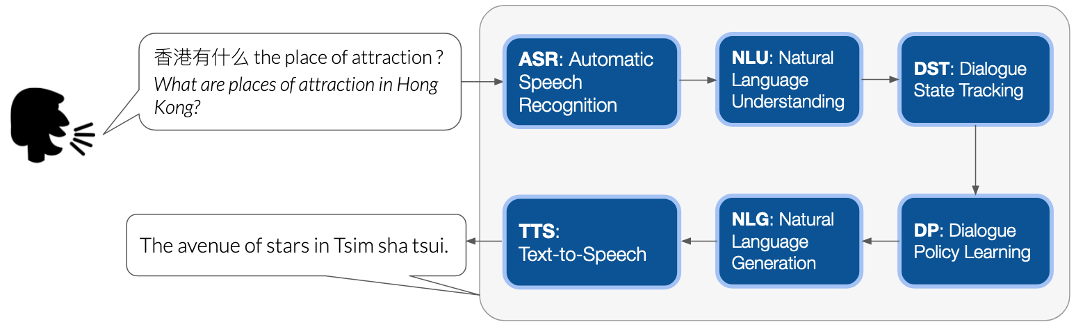
Figure 1.1: End-to-end flow of the goal-oriented dialogue system.

The following are the major challenges to developing code-switching models:

• Incorporating linguistics theory: Most research on code-switching focuses on finding constraints in the way monolingual grammars interact with each other to produce well-formed code-switched speech, and building code-switching grammars so that linguists can understand how code-switches are triggered. Using this knowledge, we can generate synthetic code-switching sentences as weak signals for the model, and thereby boost the performance of code-switching models [1, 22, 23, 24].

• Leveraging monolingual data: Lack of data is a critical issue for training code-switching models. With the rise in the number of multilingual speakers, speech recognition systems that support different languages are in demand. However, most such systems are unable to support numerous low-resource languages, particularly mixed languages. The data scarcity of low-resource languages has been a major challenge for dialogue and speech recognition systems since they require a large amount of data to learn a robust model, and collecting training data is expensive and resource-intensive. A number of previous studies have used monolingual data as training signals for transfer learning, and these data can also be used in the form of pre-training.

• Improving code-switching representations: Learning a model to understand mixed language text or speech is very important to building better bilingual or multilingual systems that are robust to different language mixing styles. This will benefit dialogue systems and speech applications, such as virtual assistants [25]. However, training a robust code-switching ASR model has been a challenging task for decades due to data scarcity. One way to enable low-resource language training is by first applying transfer learning methods that can efficiently transfer knowledge from high-resource languages [26] and then generating synthetic speech data from monolingual resources [27, 28]. However, these methods are not guaranteed to generate natural code-switching speech or text. Another line of work explores the feasibility of leveraging large monolingual speech data in the pre-training, and applying fine-tuning on the model using a limited source of code-switching data, which has been found useful to improve performance [23, 28]. However, the transferability of these pre-training approaches is not optimized to extract useful knowledge from each individual languages in the context of code-switching, and even after the fine-tuning step, the model forgets the previously learned monolingual tasks. One of the most intuitive ideas to create a multilingual representation is using pre-trained multilingual language models, such as multilingual BERT [29], as a feature extractor. However, these models are not trained for code-switching, which makes them a poor option for this case.

Traditionally, the approach to solving the low-resource issue in code-switching is to apply linguistic theories to the statistical model. Linguists have studied the code-switching phenomenon and proposed a number of theories, since code-switching is not produced indiscriminately, but follows syntactic constraints [30, 31, 5, 32]. Linguists have formulated various constraints to define a general rule for code-switching. However, these constraints cannot be postulated as a universal rule for all code-switching scenarios, especially for languages that are syntactically divergent [33], such as English and Mandarin, since they have word alignments with an inverted order. Variations of code-switching also exist, and many of them are influenced by traditions, beliefs, and normative values in the respective communities [34]. Studies describe that code-switching is dynamic across communities or regions and each has its own way to mix languages [35, 36]. Thus, building a statistical code-switching model is challenging due to complexity in the grammatical structure and localization of code-switching styles. Another shortcoming of this approach is the limitation of syntactic parsers for mixed language sentences, which are currently unreliable.

In this thesis, we address the different challenges mentioned above. We propose language-agnostic approaches that are not dependent on particular languages to improve the generalization of our models on code-switched data. We first introduce a multi-task learning to benefit from syntactic information in neural-based language models, so that the models share a syntactical representation of languages to leverage linguistic information and tackle the low-resource data issue. Then, we present two data augmentation methods to obtain synthetic code-switched training data by (1) aligning parallel sentences and applying linguistic constraints to check valid sentences and (2) using a copy-mechanism to learn how to generate code-switching sentences by sampling from the real distribution of code-switching data. The copy mechanism learns how to combine words from parallel sentences and identifies when to switch from one language to the other. We add the generated data on top of the training data and explore several fine-tuning strategies to improve code-switched language models. Next, we introduce new meta-embedding approaches to effectively transfer information from rich monolingual data to address the lack of code-switching data in different downstream NLP and speech recognition tasks. We introduce Meta-Transfer Learning to transfer-learn on a code-switched speech recognition system in a low-resource setting by judiciously extracting information from high-resource monolingual datasets. Finally, we propose a new representation learning method to represent code-switching data by learning how to transfer and acquire useful knowledge learned from other languages.

1.2 Thesis Outline

The contents of this thesis are organized around code-switching, and our experiments are focused on code-switching NLP and speech tasks. The rest of the thesis is divided into six chapters and organized as follows:

• Chapter 2 introduces the background and important related work on linguistic theories of code-switching. Then, we discuss applications of code-switching, such as language modeling, speech recognition, and sequence labeling, and we also explain how to compute code-switching complexity. This chapter presents the fundamentals required to understand the rest of the thesis.

• Chapter 3 examines approaches to training language models for code-switching by leveraging linguistic theories and neural network language models. We propose a data augmentation method to increase the variance of the corpus with linguistic theory and a model-based approach.

• Chapter 4 presents approaches to train language models in a multi-task training that leverages syntactic information. We train our model by jointly learning the language modeling task and part-of-speech (POS) sequence tagging task on code-switched utterances. We incorporate language information into POS tags to create bilingual tags that distinguish between languages.

• Chapter 5 introduces approaches to train code-switching speech recognition by transfer learning methods. Our methods apply meta-learning by judiciously extracting information from high-resource monolingual datasets. The optimization conditions the model to retrieve useful learned information that is focused on the code-switching domain.

• Chapter 6 discusses the state-of-the-art multilingual representation learning methods for code-switched named entity recognition (NER). We introduce meta-embeddings, considering the commonalities across languages and compositionality. We find that this method is language-agnostic, and it is very effective and efficient compared to large contextual language models on the code-switching domain. We also conduct a study to measure the effectiveness and efficiency of the multilingual models to see their capability and adaptability in the code-switching setting.

• Chapter 7 summarizes this thesis and the significance of the transfer learning approaches, and discusses possible future research directions.

Chapter 2 Background and Preliminaries

2.1 Overview

In this chapter, we provide a literature review and background knowledge on the theoretical and computational linguistics aspects of code-switching that are fundamental to our work. We present the common linguistic models on code-switching that can later be applied to statistical models. We also introduce contemporary studies on NLP and speech recognition with code-switching data, such as language identification, language modeling, speech recognition, and sequence tagging. Lastly, we show metrics to evaluate and measure the code-switching complexity of a corpus.

2.2 Linguistic Models of Code-Switching

Early studies on code-switching formalize linguistic assumptions about how people learn to switch from one language to another by observing the grammar and syntax. The rules mainly compare the grammars of two languages, and find the asymmetric relations between them. They investigate trigger words that activates the switch, such as POS tags and proper nouns that have strong relationships with code-switching [37]. From the qualitative perspective, there are three well-established linguistic theories that are commonly used in the linguistic world [38]: (1) the free morpheme constraint, (2) the matrix language-frame model, and (3) the equivalence constraint. These three theories will be discussed in the following.

2.2.1 Free Morpheme Constraint

Morphemes can be classified into two types: free morphemes and bound morphemes. Free morphemes are those that can stand alone to function as words, while bound morphemes are those that can only be attached to another part of a word. Poplack [5] proposes that code-switching will occur in any constituent in discourse if that constituent is not a bound morpheme. Basically, this work states a condition that a code-switch may occur between a free and a bound morpheme if and only if the bound morpheme is phonologically integrated into the language. For example, in Spanish-English,the utterance

Utterance: And what a tertuliait was, Dios mio!

Translation: And what a gathering it was, my God!.

is acceptable under the free morpheme constraint, since “Dios mio” is a bound morpheme, unlike the following sentence:

Utterance: *Estaba type-ando su ensayo.

Translation: She was type-ing her essay.

2.2.2 Equivalence Constraint

We define the dominant language as the matrix language and the contributing language as the embedded language. According to the equivalence constraint (EC) theory, code-switches will tend to occur at points in a discourse where the juxtaposition of the matrix language ($L_{1}$) and embedded language ($L_{2}$) elements does not violate a syntactic rule of either language [5, 39]. For example, we have an example of parallel sentences in English and Chinese:

$L_{1}$ (English): this is actually belonged to simplified chinese

$L_{2}$ (Chinese): 这个 其实 是 属于 简体 中文.

We align words for which the constituents from the two languages map onto each other [5]. Figure 2.1 shows an example where the switches are permissible. Solid lines show the alignment between the matrix language (top) and the embedded language (bottom). The dotted lines denote impermissible switching.

Figure 2.1: Example of equivalence constraint using aligner on English-Chinese data.

We can also interpret the EC theory by defining context-free grammars $G_{1}$ and $G_{2}$ of $L_{1}$ and $L_{2}$, respectively. This assumes that every non-terminal category in G1 has a corresponding non-terminal category in G2, as stated by Pratapa et al. [1]. In their implementation, the sentences are parsed using a monolingual syntactic parser.

$L_{1}$ (English): She lives in a white house

$L_{2}$ (Spanish): Elle vive en una casa blanca.

Figure 2.2 represents the sentences above in a tree form, where (a) is the original English sentence, (b) the original Spanish sentence, (c) the incorrectly code-mixed sentence, and (d) the correctly code-mixed sentence that satisfies the EC theory.

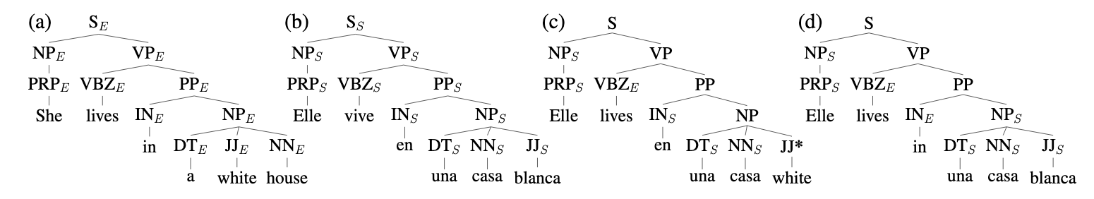
Figure 2.2: Example of equivalence constraint on English-Spanish using syntactic parsers [1].

However, this method relies on the quality of the parser, and it is difficult to apply to languages with distant grammatical structures, like English and Chinese, due to the large difference in the syntactic tags.

2.2.3 Matrix Language-Frame Model

The matrix language-frame (MLF) model states the grammatical procedures to produce code-switching sentences [40]. The model defines the matrix language as the primary language (L1) and embedded language as the embedded language (L2) that is inserted into the morphosyntactic frame of the matrix language. The MLF model defines three different constituents: L1 islands, L2 islands, and both L1 and L2 constituents. This framework also introduces the blocking hypothesis, which states that any embedded language morpheme, which is not congruent with the matrix language is blocked.

2.3 End-to-end Speech Recognition

The ASR system is the first step in the pipeline of systems in applications such as conversational agents, so any errors made by the ASR system can propagate through the wider system and lead to failures in interactions. Attempts have been made to approach the problem of code-switched ASR from the acoustic, language, and pronunciation modeling perspectives. The research on speech recognition has been further developed from modularized systems into end-to-end systems that combine acoustic, pronunciation, and language models into a single monolithic model. The recent advancement in sequence-to-sequence models has shown promising results in training monolingual ASR systems. Two common architectures are widely used for end-to-end speech recognition: connectionist temporal classification (CTC) [41] and encoder-decoder models [42, 43, 28, 44]. Further explorations on end-to-end architectures have been made by jointly training both of these architectures in a multi-task hybrid fashion [45, 46], and they have found that these architectures improve the performance of the overall model.

2.3.1 RNN-based Encoder-Decoder Model

The first-ever proposed end-to-end encoder-decoder ASR model, Listen-Attend-Spell (LAS) [47], uses a recurrent neural network (RNN) as its encoder and decoder components. The LAS model introduces two components, a listener and speller, with the former acting as an acoustic model that accepts filter bank spectra as inputs, and the latter working as the decoder that emits character outputs.

Listener

The listener uses a bidirectional long short-term memory (BiLSTM) [48, 49] with a pyramidal structure to reduce the length of the audio frames. The pyramid BiLSTM reduces the time resolution by a factor of 2, similar to Clockwork RNN [50], to address the slow convergence issue. We concatenate the outputs at consecutive steps of the current layer before feeding the concatenation to the next layer as follows:

$$h_{i}^{j}=\text{BiLSTM}(h)_{i-1}^{j},[h_{2i}^{j-1},h_{2i+1}^{j-1}]),$$ (2.1)

where $\mathbf{h}=(h_{1},h_{2},...h_{U-1},h_{U})$ is the high-level representation, and $U\leq T$, where $T$ is the length of the input sequence.

Speller

The speller is an attention-based long short-term memory (LSTM) that produces a probability distribution over the next character, conditioned on previous characters. The further equations are as follows:

$$c_{i}=\text{Attention}(s_{i},\mathbf{h}),$$ (2.2)

$$s_{i}=\text{RNN}(s_{i-1},y_{i-1},c_{i-1}),$$ (2.3)

$$P(y_{i}|\mathbf{x},y_{<i})=\text{Output}(s_{i},c_{i}).$$ (2.4)

At each time step, the attention mechanism will generate a context vector $c_{i}$, and the context $c_{i}$ contains the information of the acoustic signal that is required to generate the next character. Then, the RNN module will generate a new decoder state $s_{i}$ and pass it to the output layer to generate a character distribution $P(y_{i}|\mathbf{x},y_{<i})$. The model can be trained jointly to maximize the log probability as follows:

$$\max_{\theta}\sum_{i}{\log P(y_{i}|\mathbf{x},y^{*}_{<i};\theta)},$$ (2.5)

where $y^{*}_{<i}$ is the true labels of the previous characters. We always give transcripts for predicting the next character. In the inference time, the model finds the most likely character sequence given the audio frame inputs. The decoding process is to search the most likely sequence of given words:

$$\hat{\mathbf{y}}=\text{arg}\max_{\mathbf{y}}\log P(\mathbf{y}|\mathbf{x}).$$ (2.6)

We add a start of sentence token, <SOS>, at each time step, and apply a beam-search to collect a set of hypotheses that have an end of sentence token <EOS>. We rescore our beams with a language model score $P_{\text{LM}}(\mathbf{y})$ to improve the predictions as follows:

$$s(\mathbf{y}|\mathbf{x})=\alpha P(\mathbf{y}|\mathbf{x})+\beta\log P_{\text{LM}}(\mathbf{y}),$$ (2.7)

where $\alpha$ is the ASR model weight and $\beta$ is the language model weight.

2.3.2 Transformer-based Encoder-Decoder Model

In recent studies [43, 51, 28], transformers replace RNN modules in the ASR system since it is more efficient in terms of time and memory complexity. The RNN model has issues in parallelization, and it has to do a recursive function through the sequence length. The transformer is able to cut this dependency, allows the input to be processed in parallel, and uses an attention mechanism to attend to all tokens. Similar to the RNN model, the transformer-based model also predicts target tokens and accepts speech features as input. The transformer-based ASR architecture is illustrated in Figure 2.3.

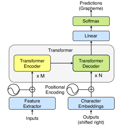
Figure 2.3: Transformer ASR model architecture.

In the following, we describe the structure of the encoder and decoder layer.

Encoder Layer

Figure 2.4 shows the structure of the encoder layer. An adapter layer is added after the layer norm and self-attention module. We also apply two residual connections after both the self-attention layer and the adapter layer:

$$\mathbf{o} =\text{SelfAttn}(\text{LayerNorm}(\mathbf{h}_{\text{enc}}^{l-1}))+\mathbf{h}_{\text{enc}}^{l-1},$$ (2.8)

$$\mathbf{h}_{\text{enc}}^{l} =\text{FeedForward}(\text{LayerNorm}(\mathbf{o})+\mathbf{o}),$$ (2.9)

where $\mathbf{h}_{\text{enc}}^{l-1}$ is the encoder hidden states of the previous layer $l-1$ and $\mathbf{h}_{\text{enc}}^{l}$ is the output of the encoder layer.

Decoder Layer

Figure 2.5 shows the structure of the decoder layer with the adapter. We place the adapter layer after the cross-attention model:

$$\mathbf{o}_{1} =\text{SelfAttn}(\text{LayerNorm}(\mathbf{h}_{\text{dec}}^{l-1}))+\mathbf{h}_{\text{dec}}^{l-1},$$ (2.10)

$$\mathbf{o}_{2} =\text{CrossAttn}(\mathbf{h}_{\text{enc}},\text{LayerNorm}(\mathbf{o}_{1}))+\mathbf{o}_{1},$$ (2.11)

$$\mathbf{h}_{\text{dec}}^{l+1} =\text{FeedForward}(\text{LayerNorm}(\mathbf{o}_{2})+\mathbf{o}_{2}),$$ (2.12)

where $\mathbf{h}_{\text{dec}}^{l-1}$ is the decoder hidden states of the previous layer, and $\mathbf{h}_{\text{dec}}^{l}$ is the output of the current layer.

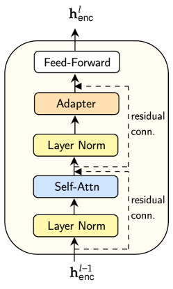
Figure 2.4: Encoder transformer structure.

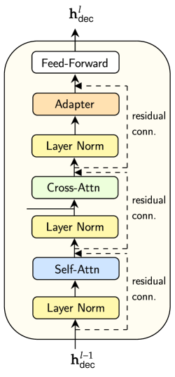
Figure 2.5: Decoder transformer structure.

The transformer model has three main components: a scaled dot-product attention, multi-head attention, and positional-wise feed-forward network.

Scaled Dot-Product Attention

The attention function is described as a mapping between a query and a set of key-value pairs to an output [52]. The weight calculated from the function is assigned to the value. Particularly for the scaled dot-product attention, we apply dot products of the queries of dimension $d_{q}$ and keys of dimension $d_{k}$. Then, we divide each of them by $\sqrt{d_{k}}$ and apply the softmax function to compute the weights. We use the weights to weigh the values of dimension $d_{v}$. Normally, we set $d_{q}=d_{k}$, and $d_{model}$ is divisible by the number of heads $h$.

$$\text{Attention}(Q,K,V)=\text{Softmax}(\frac{QK^{T}}{\sqrt{d_{k}}})V.$$ (2.13)

Multi-head Attention

Instead of using a single-head attention, we can apply multiple $h$ heads that learn the linear projections of the query, key, and value. As suggested by Vaswani et al. [52], multi-head attention is more beneficial in learning representation subspaces at different positions:

$$\text{MultiHead}(Q,K,V) =\text{Concat}(\text{head}_{1},...,\text{head}_{h})W^{O},$$ (2.14)

$$\text{head}_{i} =\text{Attention}(QW^{Q}_{i},KW^{K}_{i},VW^{V}_{i}),$$ (2.15)

where the projection matrices $W_{i}^{Q}\in\mathbb{R}^{d_{model}\times d_{q}}$, $W_{i}^{K}\in\mathbb{R}^{d_{model}\times d_{k}}$, $W_{i}^{V}\in\mathbb{R}^{d_{model}\times d_{v}}$, and $W_{i}^{O}\in\mathbb{R}^{d_{hd_{v}}\times d_{model}}$.

Position-Wise Feed-Forward Network

After the attention layers in the encoder and decoder, we add a linear layer that is applied to each position and a ReLU activation. The layer will project the input into $d_{model}$. During the implementation, we can use two convolutions with a kernel size of 1:

$$\text{FFN}(x)=\text{max}(0,xW_{1}+b_{1})W_{2}+b_{2}.$$ (2.16)

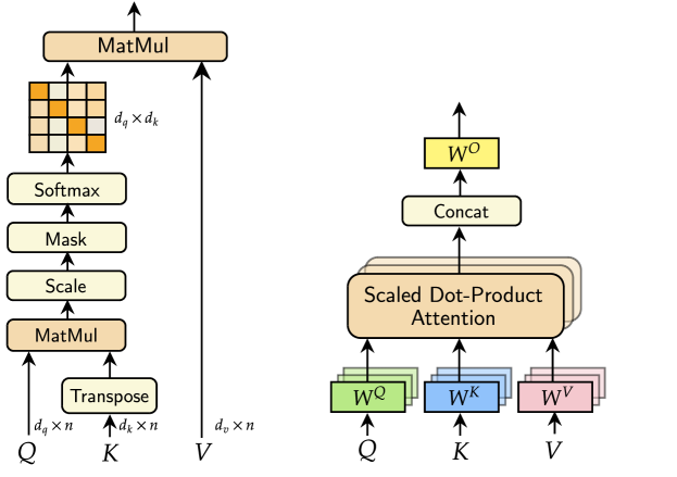
Figure 2.6: Transformer components. (left) Scaled dot-product attention. (right) Multi-head attention.

For the training, we follow the same training objective as the RNN-based model, and we apply the same inference procedure.

2.3.3 Code-Switched Speech Recognition

Since code-switching is a spoken language phenomenon, it is important for ASR systems to be able to handle code-switching speech. The initial attempts at code-switched ASR systems, focus on building HMM-based systems, where the ability to recognize the language speech frames is based on finding the language boundaries using language identification (LID). The detected monolingual frames are then passed into monolingual ASR systems [53, 54]. One way to identify the language boundaries is to recognize the monolingual speech fragments [53]. Another approach to detecting code-switching speech is to map phone sets of code-switched language pairs into IPA mappings and construct a bilingual phone set and clustered phones. This approach has been conducted on Mandarin-English [55], Ukrainian-Russian [56], and Hindi-English [57]. By applying this method, we can train code-switched ASR in a single model.

2.3.4 Evaluation Metrics

Word error rate (WER) is the standard metric for evaluating speech recognition systems, and it is determined as follows:

$$WER=\frac{INS+DEL+SUB}{N}\times 100\%,$$ (2.17)

where $INS$, $DEL$, and $SUB$ are the number of insertions, deletions, and substitutions, respectively, and $N$ is the number of words in the reference. However, for some languages, such as Chinese, or in the mixed language setting, character error rate (CER) is used instead of WER. This metric calculates the distance between two sequences as the Levenshtein distance, and the idea of using it is to minimize the distance between two tokens or the number of insertions, deletions, or substitutions required to change one token into another. Computing CER is very similar to WER, but instead of computing a word as the token, we use a character. For our code-switched ASR, we compute the overall CER and also show the individual CERs for each language.

2.4 Language Modeling

Language modeling (LM) is a fundamental task in NLP and speech systems, most notably in ASR. Basically, an LM score indicates how well the model predicts a sequence of words. A higher score means a sequence is more likely to appear in the corpus. In the ASR task, LM is utilized to enhance the speech recognition results by re-scoring the hypothesis and maximizing the posteriors. The LM assigns a joint probability over all possible word sequences $\mathbf{w}$, $P_{\text{LM}}(\mathbf{w})$. We can compute the probability by using Bayes’ theorem:

$$P_{\text{LM}}(\mathbf{w})=P(w_{1},w_{2},...,w_{n})=\prod_{i=1}^{n}P(w_{i}|w_{<i})=P(w_{1})P(w_{2}|w_{1})...P(w_{i}|w_{1},w_{2},...w_{i-1}).$$ (2.18)

2.4.1 n-gram Language Modeling

The n-gram LM applies the Markov assumption to estimate the probability of future units without looking too far into context. The assumption is that the probability of a word only depends on the previous word. The general equation for the n-gram approximation is:

$$P(w_{1}^{n})\approx\prod_{k=1}^{n}P(w_{k}|w_{k-1}).$$ (2.19)

To compute the probability of a word $w$, we can sum all n-gram counts that start with that word, and normalize the sum by the unigram count for word $w_{n-1}$ so the number of counts lies between 0 and 1:

$$P(w_{n}|w_{n-1})=\frac{C(w_{n-1}w_{n})}{C(w_{n-1})},$$ (2.20)

where $C(.)$ is the number of word combinations appearing in the data. However, this method still suffers from issues with unknown words in a test set in an unseen context. For example, when $n=3$, the probability of the word is conditioned on the previous two words. Thus, we compute the probability as follows:

$$P(w_{i}|w_{i-1},w_{i-2})=\frac{C(w_{i},w_{i-1},w_{i-2})}{C(w_{i-1},w_{i-2})}.$$ (2.21)

Assigning an unknown token with zero probability is similar to ignoring the token; thus, it is not the best choice. We can apply a smoothing approach to assign a small probability to unknown tokens using smoothing techniques, such as Kneser-Ney [58], Laplace, or Backoff smoothing.

2.4.2 Neural-Based Language Modeling

Instead of counting the frequency and using a fixed window, as in the n-gram LM, we can enlarge the window by using an RNN. The RNN model memorizes the context of the previous word and passes it to the next-token prediction. Here, we describe two neural-based LMs using an RNN and LSTM [59], an extension of the RNN model.

RNN language model

Neural-based language models normally use an RNN [60, 61, 51] as the base model. Figure 2.7 shows the unidirectional language model architecture, and we denote the model as $\theta$. Here we will also denote our input sequences as $\mathbf{x}=(x_{1},x_{2},...,x_{n-1},x_{n})$.

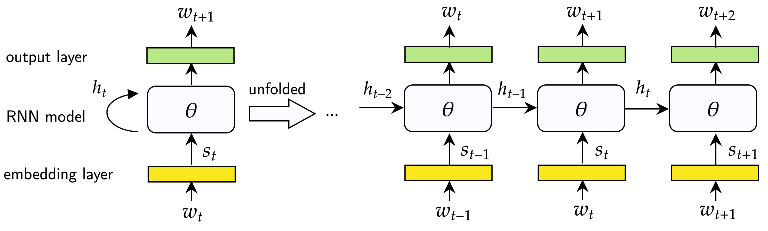
Figure 2.7: RNN language model.

A vector $\mathbf{s}_{t}$ is generated by mapping token $\mathbf{x}_{t}$ to the embedding layer $E$. The model generates an output vector $\mathbf{o}_{t}\in\mathbb{R}^{V|}$, where $|V|$ is the size of the vocabulary. Vector $\mathbf{h}_{t}$ represents the output value in the hidden layer from the previous time step and the vector is projected to the dimension as the size of the vocabulary. The softmax function is applied to $\mathbf{o}_{t}$ for normalization to output the probability distribution. The RNN model is trained using backpropagation. The outputs of the layer are computed as follows:

$$\mathbf{s}_{t} =E\mathbf{x}_{t},$$ (2.22)

$$\mathbf{h}_{t} =\sigma(\mathbf{W}_{h}\mathbf{h}_{t-1}+\mathbf{W}_{i}s_{t}+b_{1}),$$ (2.23)

$$\mathbf{o}_{t} =\mathbf{W}_{o}\mathbf{h}_{t}+b_{2},$$ (2.24)

$$\mathbf{o}_{t} =\text{Softmax}(\mathbf{o}_{t}),$$ (2.25)

$$\text{Softmax}(z) =\frac{e^{z}}{\sum_{k}e_{k}^{z}},$$ (2.26)

where $\mathbf{W}_{h}$ and $\mathbf{W}_{i}$ are the learned weights.

LSTM language model

LSTM language models [59, 62, 51] are parameterized with two large matrices, $\mathbf{W}_{i}$, and $\mathbf{W}_{h}$. The LSTM captures long-term dependencies in the input and avoids the exploding/vanishing gradient problems of the standard RNN. The gating layers control the information flow within the network and decide which information to keep, discard, or update in the memory. The following recurrent equations show the LSTM dynamics:

$$\small\begin{pmatrix}\mathbf{i}_{t}\\ \mathbf{f}_{t}\\ \mathbf{o}_{t}\\ \mathbf{\hat{c}}_{t}\end{pmatrix} =\begin{pmatrix}\sigma\\ \sigma\\ \sigma\\ \text{tanh}\end{pmatrix}\begin{pmatrix}\mathbf{W}_{i}&\mathbf{W}_{h}\end{pmatrix}\begin{pmatrix}\mathbf{s}_{t}\\ \mathbf{h}_{t-1}\end{pmatrix},$$ (2.27)

$$\small\mathbf{W}_{i} =\begin{pmatrix}\mathbf{W}_{i}^{i}\\ \mathbf{W}_{i}^{f}\\ \mathbf{W}_{i}^{o}\\ \mathbf{W}_{i}^{c}\end{pmatrix},\mathbf{W}_{h}=\begin{pmatrix}\mathbf{W}_{h}^{i}\\ \mathbf{W}_{h}^{f}\\ \mathbf{W}_{h}^{o}\\ \mathbf{W}_{h}^{c}\end{pmatrix},$$ (2.28)

$$\mathbf{o}_{t} =\text{Softmax}(W_{o}\mathbf{o}_{t}),$$ (2.29)

where $\mathbf{s}_{t}\in\mathbb{R}^{n_{inp}}$ and $\mathbf{h}_{t}\in\mathbb{R}^{n_{dim}}$ at time $t$. Here, $\sigma(\cdot)$ and $\odot$ denote the sigmoid function and element-wise multiplication operator, respectively. The model parameters can be summarized in a compact form with $\theta=[\mathbf{W}_{i},\mathbf{W}_{h}]$, where $\mathbf{W}_{i}\in\mathbb{R}^{4*n_{inp}\times 4*n_{dim}}$, which is the input matrix, and $\mathbf{W}_{h}\in\mathbb{R}^{4*n_{dim}\times 4*n_{dim}}$, which is the hidden matrix. Note that we often refer to $\mathbf{W}_{i}$ as additive recurrence and $\mathbf{W}_{h}$ as multiplicative recurrence. Then, $\mathbf{o}_{t}\in\mathbb{R}^{|V|}$ is generated by the model, and we apply the softmax function to compute the probability distribution.

2.4.3 Code-Switched Language Modeling

It is very well known that the larger the dataset we use for training, the better the language model we can get. However, in the code-switching domain, it is very hard to collect high-quality data and it is very expensive to acquire. One possible source of data is social media, but these data still need to be annotated. There are several approaches to annotate code-switched sentences using LID and syntactic information. We can classify the current research directions into four categories:

Linguistic features

Linguistic features are commonly used in language model training [63, 64] and are generally a combination of both semantic and syntactic features [65], which give more semantic and syntactic information to the model.  Adel et al. [65] show that the features can be used as code-switch triggers, such as POS, brown clusters, and open class words.

Data augmentation

The goal of this approach is to increase the amount of code-switching data by generating new samples to address the data limitation issue. Traditionally in computational linguistics, we depend on linguistic theories to generate more code-switching samples. The theories are used to constraint the generation so that the results are more natural and human-like. The first work to study the use of linguistic theories for this purpose is by Li and Fung [24], who used the assumption of the equivalence constraint [24, 1, 66] and functional head constraint [67]. Instead of using linguistic theories, other studies have developed methods that use a neural-based approach for data augmentation to learn the code-switching data distribution, such as SeqGAN [68] and an encoder-decoder model with a copy mechanism [28].

Transfer learning methods

Leveraging out-of-domain data in the training is a common technique to improve performance and generalization in the code-switching domain. One of the approaches is to apply pre-training on monolingual data before fine-tuning the data with code-switching data using multi-task learning [24, 28].

Deep learning architectures

A number of studies have applied deep learning models to code-switched models. The first neural-based language model was proposed by Adel et al. [63] using an RNNLM model. They later [69] proposed an ensemble model to combine factoid RNNLM with n-gram language models. Further work on deep learning for code-switching was done by Choudhury et al. [70], who introduce curriculum learning for training code-switched models to train a network with monolingual training instances, Garg et al. [71], who propose DualRNN, a model with two RNN components that focus on each of two languages, and Chandu et al. [72], who use language information in an RNN-based language model to help learn code-switching points.

2.4.4 Evaluation Metrics

The perplexity (PPL) is a standard metric to evaluate a language model. It measures how likely a sequence is to occur [73, 74], and is formulated as follows:

$$\text{PPL}(\mathbf{x})=P(\mathbf{x}_{1},\mathbf{x}_{2},...,\mathbf{x}_{N})^{-\frac{1}{N}}=\sqrt[N]{\frac{1}{P(\mathbf{x}_{1},\mathbf{x}_{2},...,\mathbf{x}_{N})}},$$ (2.30)

where $\text{x}=(\mathbf{x}_{1},\mathbf{x}_{2},...,\mathbf{x}_{N})$ is a word sequence and $N$ is the sequence length. In the context of code-switching, we calculate PPL differently for Chinese and English. In Chinese, we use characters, while in English we use words. The reason is that some Chinese words are not well tokenized by the Chinese tokenizer, as mentioned by Garg et al. [75] and Winata et al. [28], and tokenization results are not consistent. Using characters instead of words in Chinese can alleviate word boundary issues. The PPL is calculated by taking the exponential of the sum of losses. To show the effectiveness of our approach in calculating the probability of the switching, we split the perplexity computation into monolingual segments (en-en) and (zh-zh), and code-switching segments (en-zh) and (zh-en).

2.5 Sequence Labeling

Sequence labeling is the key task for NLU. The task is very useful in many NLP applications, for instance, in a conversational virtual agent to detect slot values or named entities from the user inputs. Notably, in code-switching, the sequence labeling task is more challenging since there might be ambiguity in the semantics, and learning the representation for code-switched sentences is not trivial. Sequence labeling comprises a variety of sub-tasks, such as LID, NER, and POS tagging, which will be discussed below.

2.5.1 Language Identification

LID is a task to identify the language of each word within an utterance. Identifying language in code-switched data is crucial since the boundary separates two sub-utterances with different languages. Conventional LID systems operate at the sentence level, which leads to the requirement of word-level LID. Multiple cues, including acoustic, prosodic, and phonetic features are useful features for LID [76]. A couple of shared tasks, EMNLP 2014 [77] and EMNLP 2016 [78], have played an essential role in establishing datasets for LID.

2.5.2 Named Entity Recognition

NER datasets for code-switching are similar to LID datasets, with word-level annotations. The NER data for code-switching are tweets crawled from online social media for Spanish-English and Arabic-English, and they were compiled and released as a shared task in ACL 2018 [79]. In the shared task, Attia et al. [80] augment convolutional-based character embeddings and external resources, such as gazetteers and brown clusters into a BiLSTM with a conditional random field (CRF) model, while Geetha et al. [81] also incorporate external resources like gazetteers and cross-lingual embeddings, such as MUSE [82]. Winata et al. [19] introduce a set of pre-processing methods to reduce the out-of-vocabulary (OOV) rate on the code-switching data, and bilingual character embeddings using an RNN model.

2.5.3 Part-of-Speech Tagging

POS tagging datasets consist of code-switched sentences tagged at the word-level with POS information. Similar to NER, the datasets are collected from social media on Spanish-English data [83] and Hindi-English data [84]. This task is an important linguistic component that is used for constituency and dependency parsing. In this task,  Vyas et al. [11] use a CRF-based tagger and a Twitter POS tagger in order to tag sequences of mixed language, while Solorio and Liu [83] explore monolingual resources to train taggers.

2.6 Representation Learning in NLP

2.6.1 Word Embeddings

Learning a representation through embedding is a fundamental technique to capture latent word semantics [85]. In the early stages of research on this topic, Word2Vec embeddings [86, 87] were the first model to be proposed to the NLP community for word-level representation learning, and interestingly, the embeddings can captures semantics of a word in the form of a vector. The Word2Vec model is used to map words in the discrete space into a vector representation in the continuous space. The goal of building the embeddings is to learn high-quality word vectors from large datasets. There are two training techniques to train word representations: The Skip-gram and continuous bag of words (CBOW) model [86]. The Skip-gram is used to predict the context words for a given word by training, while CBOW applies a reverse technique to Skip-gram: it predicts the word by providing the context as input.

Another type of word embedding is GloVe [88], which leverages statistical information by training only on the nonzero elements in a word-word co-occurrence matrix, instead of on the entire sparse matrix or individual context windows. The model produces a word vector space with a meaningful sub-structure. Standard word vectors ignore the rich structures of languages, and do not consider rare or misspelled words; thus, FastText [89, 90, 91] was proposed to address the issue. If a word is unknown, the representations are formed by summing all vectors. To better capture the morphology of the language and address the out-of-vocabulary (OOV) issue, subwords and characters have been commonly used to replace words. One of the commonly used subword embeddings is BPEmb [92], that utilizes byte pair encoding (BPE), a variable-length encoding that views the text as a sequence of symbols and iteratively merges the most frequent symbol pair into a new symbol.

2.6.2 Contextualized Language Models

A deep contextualized model has been proposed to learn representations [93]. Different from word embeddings, it uses a BiLSTM to capture context-dependent aspects of the word semantics to perform well on sequence labeling tasks such as NER and POS tagging. Recently, the BERT model [94] advanced the state-of-the-art on various NLP tasks. It uses attention models to capture multi-directional representations, instead of using a shallow bidirectional left-to-right and right-to-left, as well as WordPiece [95] as the vocabulary to address the OOV issue. A multilingual extension of BERT, mBERT, has shown itself to be very effective on multilingual and cross-lingual NLP tasks [96, 97, 98, 99], speech recognition [46], and low-resource languages [100]. This multilingual model helps to improve the generalization of different languages since they are trained on large monolingual datasets. However, training a model using only monolingual datasets does not help in code-switching tasks since the model is not informed of the interlingual alignments.

2.6.3 Representation Learning for Code-Switching Tasks

To represent a code-switched sentence, we need a bilingual or multilingual model that understands both languages and has the cross-lingual alignment between words in different languages that have similar semantics. Following are the current methods addressing code-switching representation:

Bilingual Correlation-Based Embeddings (BiCCA)

Faruqui and Dyer [101] propose canonical correlation analysis, which measures the linear relationship between two embeddings from different languages, finds the two best projection vectors with respect to the correlation, and projects the embeddings into the same dimension space. These word representations are more suitable for encoding a word’s semantics than its syntactic information [101].

Bilingual Compositional Model (BiCVM)

Hermann and Blunsom [102] propose to learn a multilingual representation using parallel sentences and minimize the energy between semantically similar sentences. They use a noise-constrastive large-margin update to ensure that representations of non-aligned sentences have a certain margin between each other.

BiSkip

Luong et al. [103] extend the Skip-gram [87] to the bilingual setting, where the model learns to predict word contexts cross-lingually, or in other words, to align words in L1 to corresponding words in L2, and vice versa.

MUSE

Lample et al. [82]and Conneau et al. [104] propose to learn bilingual word embeddings by an unsupervised method that can be used for unsupervised machine translation and cross-lingual tasks. The model learns a mapping from the source to target space using adversarial training and Procustes alignment [105].

Synthetic Data (GCM) Embeddings

Pratapa et al. [106] propose to train Skip-gram embeddings from synthetic code-switched data generated by Pratapa et al. [1]. They show that GCM improves syntactic and semantic code-switching tasks.

Char2Subword

Recently,  Aguilar et al. [3] have proposed the Char2Subword module that builds representations from characters out of the subword vocabulary and they use the module to replace subword embeddings. This model is also robust to typographical errors, such as the misspellings, inflection and casing that are mainly found in social media text. They provide a comprehensive empirical study on a variety of code-switching tasks, such as LID, NER, and POS tagging.

2.7 Complexity Metrics

Two metrics are commonly used for computing the amount of code-switching in a sequence: the switch-point fraction (SPF) and code mixing index (CMI).

2.7.1 Switch-Point Fraction

The SPF calculates the number of switch-points in a sentence divided by the total number of word boundaries [1]. We define switch-point as a point within a sentence at which the languages of words on either side are different. It is formulated as follows:

$$SPF(W)=\frac{P(W)}{N(W)},$$ (2.31)

where $N(W)$ is the number of tokens of utterance $W$, and $P(W)$ is the number of code-switching points in utterance $W$.

2.7.2 Code Mixing Index

The CMI counts the number of switches in a corpus [107]. It can be computed at the utterance level by finding the most frequent language in the utterance and then counting the frequency of the words belonging to all other languages present. We compute this metric at the corpus level by averaging all the sentences in a corpus. The computation is shown as follows:

$$CMI(W)=\frac{N(W)-max(\ell_{i}\in\ell\{t_{\ell_{i}}(W)\})+P(W)}{N(W)},$$ (2.32)

where $CMI(W)$ is the score of the code mixing index of utterance $W$, $N(W)$ is the number of tokens of utterance $W$, $t_{\ell_{i}}$ is the tokens in language $\ell_{i}$, and $P(W)$ is the number of code-switching points in utterance $W$. We compute this metric at the corpus level by averaging the values for all sentences.

Chapter 3 Linguistically-Driven Code-Switched Language Modeling

The lack of data problem is the main issue for building a robust code-switching model. Although, a vast number of monolingual data are available in social media, they do not follow the same patterns as code-switching speech. Traditionally, this issue is tackled by generating synthetic code-switched data using assumptions from linguistic constraints. However, relying on linguistic constraints may only benefit language pairs that have been heavily investigated in linguistic research. Linguistic constraints are also dependent on syntactic parsers that are unreliable on distant languages, such as English and Mandarin.

In this chapter, we introduce transfer learning approaches that use monolingual data for domain adaptation, and a small number of code-switching data for fine-tuning. We propose language-agnostic computational approaches to generate code-switching data that can be extended to any language pairs using two different methods: (1) leveraging the equivalence constraint to validate the generated data without any external parsers, and (2) learning the data distribution of code-switching data using a neural-based model with a copy mechanism. Then, we take the augmented data to train a language model.

3.1 Model Description

3.1.1 Data Augmentation Using Equivalence Constraint

Existing methods of data augmentation apply EC theory to generate code-switching sentences. The methods in Li and Fung [24] and Pratapa et al. [1] may suffer performance issues as they receive erroneous results from the word aligner and POS tagger, causing misclassification that affects the quality of the alignment. Thus, these approaches are not reliable or effective. Recently,  Garg et al. [75] proposed a SeqGAN-based model which learns how to generate new synthetic code-switching sentences. However, the distribution of the generated sentences is very different from real code-switching data, which leads to underperformance. Studies on the EC [5, 39] show that code-switching only occurs where it does not violate the syntactic rules of either language. Pratapa et al. [1] apply the EC in English-Spanish LM with a strong assumption. However, we are working with English and Chinese, which have distinctive grammar structures (e.g., POS tags), so applying a constituency parser would give us erroneous results. Thus, we simplify sentences into a linear structure, and we allow lexical substitution on non-crossing alignments between parallel sentences.

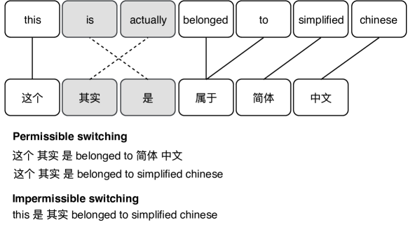
Figure 3.1: Example of equivalence constraint.

Figure 3.1 shows an example of the EC in English and Chinese. Solid lines show the alignment between the matrix language (top) and the embedded language (bottom). The dotted lines denote impermissible switching. Alignments between an $L_{1}$ sentence and an $L_{2}$ sentence comprise a source vector with indices $u_{t}=\{a_{1},a_{2},...,a_{m}\}\in\mathbb{W}^{m}$ that has a corresponding target vector $v_{t}=\{b_{1},b_{2},...,b_{n}\}\in\mathbb{W}^{n}$, where $u$ is a vector of indices sorted in an ascending order. The alignment between $a_{i}$ and $b_{i}$ does not satisfy the constraint if there exists a pair of $a_{j}$ and $b_{j}$ where ($a_{i}<a_{j}$ and $b_{i}>b_{j}$) or ($a_{i}>a_{j}$ and $b_{i}<b_{j}$). If the switch occurs at this point, it changes the grammatical order in both languages; thus, this switch is not acceptable. During the generation step, we allow any switches that do not violate the constraint. We propose to generate synthetic code-switching data by the following steps:

1. Align the $L_{1}$ sentences $Q$ and $L_{2}$ sentences $E$ using fast_align  [108]. We use the mapping from the $L_{1}$ sentences to the $L_{2}$ sentences.

2. Permute alignments from step (1) and use them to generate new sequences by replacing the phrase in the $L_{1}$ sentence with the aligned phrase in the $L_{2}$ sentence.

3. Evaluate generated sequences from step (2) if they satisfy the EC theory.

3.1.2 Neural-Based Data Augmentation

We introduce a neural-based code-switching data generator model using the pointer generator model (Pointer-Gen) [109] to learn code-switching constraints from a limited source of code-switching data and leverage their translations in both languages [28, 66]. Intuitively, the copy mechanism can be formulated as an end-to-end solution to copy words from parallel monolingual sentences by aligning and reordering the word positions to form a grammatical code-switching sentence. We remove the dependence on the aligner or tagger, and generate new sentences with a similar distribution to the original dataset.

Initially, Pointer-Gen [109] was proposed to learn when to copy words directly from the input to the output in text summarization, and it has since been successfully applied to other NLP tasks, such as comment generation [110]. Pointer-Gen leverages the information from the input to ensure high-quality generation, especially when the output sequence consists of elements from the input sequence, such as code-switching sequences.

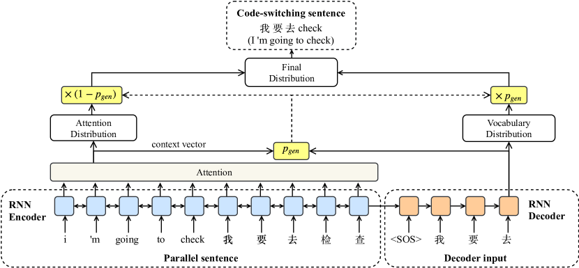
Figure 3.2: Pointer-Gen model, which includes an RNN encoder and RNN decoder. The parallel sentence is the input of the encoder, and in each decoding step, the decoder generates a new token.

We propose to use Pointer-Gen by leveraging parallel monolingual sentences to generate code-switching sentences. The approach is depicted in Figure 3.2. Pointer-Gen is trained from concatenated sequences of parallel sentences to generate code-switching sentences, constrained by code-switching text. The words of the input are fed into the encoder. Intuitively, the copy mechanism can be formulated as an end-to-end solution to copy words from parallel monolingual sentences by aligning and reordering the word positions to form a grammatical code-switching sentence. This method removes the dependence on the aligner or tagger, and generates new sentences with a similar distribution to the original dataset. Interestingly, this method can learn the alignment effectively without a word aligner or tagger. As an additional advantage, we demonstrate its interpretability by showing the attention weights learned by the model that represent the code-switching constraints.

We use a BiLSTM, which produces hidden state $h_{t}$ in each step $t$. The decoder is a unidirectional LSTM receiving the word embedding of the previous word. For each decoding step, a generation probability $p_{gen}$ $\in$ [0,1] is calculated, which weights the probability of generating words from the vocabulary, and copying words from the source text. $p_{gen}$ is a soft gating probability to decide whether to generate the next token from the decoder or to copy the word from the input instead. The attention distribution $a_{t}$ is a standard attention with general scoring [111]. It considers all encoder hidden states to derive the context vector. The vocabulary distribution $P_{voc}(w)$ is calculated by concatenating the decoder state $s_{t}$ and the context vector $h_{t}^{*}$:

$$p_{gen}=\sigma(w_{h^{*}}^{T}h_{t}^{*}+w_{s}^{T}s_{t}+w_{x}^{T}x_{t}+b_{ptr}),$$ (3.1)

where $w_{h^{*}},w_{s},$ and $w_{x}$ are trainable parameters and $b_{ptr}$ is the scalar bias. The vocabulary distribution $P_{voc}(w)$ and the attention distribution $a^{t}$ are weighted and summed to obtain the final distribution $P(w)$, which is calculated as follows:

$$P(w)=p_{gen}P_{voc}(w)+(1-p_{gen})\sum_{i:w_{i}=w}{a_{i}^{t}}.$$ (3.2)

We use a beam search to select the $N$-best code-switching sentences.

3.1.3 Language Modeling

We generate data using the EC theory and Pointer-Gen. We also compare our methods with SeqGAN [75] as baseline. To find the best way of leveraging the generated data, we compare training strategies as follows:

$$\textbf{(1)}\text{ rCS},\textbf{(2a)}\text{ EC},\textbf{(2b)}\text{ SeqGAN},$$

$$\textbf{(2c)}\text{ Pointer-Gen},\textbf{ (3a)}\text{ EC \& rCS},$$

$$\textbf{(3b)}\text{ SeqGAN \& rCS},\textbf{ (3c)}\text{ Pointer-Gen \& rCS}$$

$$\textbf{(4a)}\text{ EC}\rightarrow\text{rCS}\textbf{ (4b)}\text{ SeqGAN}\rightarrow\text{rCS},$$

$$\textbf{(4c)}\text{ Pointer-Gen}\rightarrow\text{rCS}$$

(1) is training with real code-switching data; (2a–2c) are training with only augmented data; (3a–3c) are training with the concatenation of augmented data with rCS; and (4a–4c) are running a two-step training, first training the model only with augmented data and then fine-tuning with rCS. Our early hypothesis is that the results from (2a) and (2b) will not be as good as the baseline, but when we combine them, they will outperform the baseline. We expect the result of (2c) to be on par with (1), since Pointer-Gen learns patterns from the rCS dataset, and generates sequences with similar code-switching points.

We use a stacked LSTM model to train our language models. The LSTM model is trained using a standard cross-entropy to predict the next token.

3.2 Experimental Setup

3.2.1 Datasets

In this section, we use three datasets. First, we use speech data from SEAME (South East Asia Mandarin-English), [112], a conversational English-Mandarin Chinese code-switching speech corpus that consists of spontaneously spoken interviews and conversations. This dataset consists of two phases. Phase I is the first data collected in the process, while Phase II data consists of all data from Phase I with additional data collected afterwards. Thus, we choose the Phase II dataset. Table 3.1 shows the statistics of the dataset, which is split by speaker ID. We tokenize the tokens in the transcription using the Stanford NLP toolkit [113]. The other two datasets are monolingual speech datasets, HKUST [114], comprising spontaneous Mandarin Chinese telephone speech recordings, and Common Voice, an open-accented English dataset collected by Mozilla. We split Chinese words into characters to avoid word boundary issues, and generate $L_{1}$ sentences and $L_{2}$ sentences by translating the training set of SEAME Phase II into English and Chinese using the Google NMT system. Then, we use them to generate 270,531 new pieces of code-switching data, which is thrice the number of the training sets.

Table 3.1: Data statistics of SEAME Phase II.

	Train	Dev	Test
# Speakers	138	8	8
# Duration (hr)	100.58	5.56	5.25
# Utterances	90,177	5,722	4,654
# Tokens	1.2M	65K	60K
CMI	0.18	0.22	0.19
SPF	0.15	0.19	0.17

3.2.2 Training

In this section, we present the settings we use to generate code-switching data, and train our language model and end-to-end ASR.

SeqGAN

We implement the SeqGAN model using a PyTorch implementation as our baseline, and use our best trained language model baseline as the generator in SeqGAN. We sample 270,531 sentences from the generator, thrice the number of the code-switched training data (with a maximum sentence length of 20).

Pointer-Gen

The pointer-generator model has 500-dimensional hidden states. We use 50k words as our vocabulary for the source and target, and optimize the training by Stochastic Gradient Descent (SGD) with an initial learning rate of 1.0 and decay of 0.5. We generate the three best sequences using beam search with five beams, and sample 270,531 sentences, thrice the number of the code-switched training data.

EC

We generate 270,531 sentences, thrice the number of the code-switched training data. To make a fair comparison, we limit the number of switches to two for each sentence to get a similar number of code-switches (SPF and CMI) to Pointer-Gen.

Language Model

In this work, we focus on sentence generation, so we evaluate our data with the same two-layer LSTM language model for comparison. It is trained using a two-layer LSTM with a hidden size of 200 and is unrolled for 35 steps. The embedding size is equal to the LSTM hidden size for weight tying [115]. We optimize our model using SGD with an initial learning rate of 20. If there is no improvement during the evaluation, we reduce the learning rate by a factor of 0.75. In each step, we apply a dropout to both the embedding layer and recurrent network. The gradient is clipped to a maximum of 0.25. We optimize the validation loss and apply an early stopping procedure after five iterations without any improvements. In the fine-tuning step of training strategies (4a–4c), the initial learning rate is set to 1.

3.2.3 Evaluation Metrics

We use token-level perplexity (PPL) to measure the performance of our models. For the language model, we calculate the PPL of characters in Mandarin Chinese and words in English. The reason is that some Chinese words inside the SEAME corpus are not well tokenized, and tokenization results are not consistent. Using characters instead of words in Chinese can alleviate word boundary issues. The PPL is calculated by taking the exponential of the sum of losses. To show the effectiveness of our approach in calculating the probability of the switching, we split the PPL computation into monolingual segments (en-en) and (zh-zh), and code-switching segments (en-zh) and (zh-en).

Table 3.2: Statistics of the generated data. The table shows the number of utterances and words, code-switches ratio, and percentage of new n-grams.

	EC	SeqGAN	Pointer-Gen
# Utterances	270,531	270,531	270,531
# Words	3,040,202	2,981,078	2,922,941
new unigram	13.63%	34.67%	4.67%
new bigram	69.43%	80.33%	46.57%
new trigram	99.73%	141.56%	69.38%
new four-gram	121.04%	182.89%	85.07%
CMI	0.25	0.13	0.25
SPF	0.17	0.2	0.17

3.3 Results and Discussion

3.3.1 Code-Switched Data Generation

As shown in Table 3.2, we generate new n-grams including code-switching phrases. This leads us to a more robust model, trained with both generated data and real code-switching data. We can see clearly that Pointer-Gen-generated samples have a distribution more similar to the real code-switching data compared with SeqGAN, which shows the advantage of our proposed method. Table 3.3 shows the most common English and Mandarin Chinese POS tags that trigger code-switching. The distribution of word triggers in the Pointer-Gen data are similar to the real code-switching data, indicating our model’s ability to learn similar code-switching points. Nouns are the most frequent English word triggers. They are used to construct an optimal interaction by using cognate words and to avoid confusion. Also, English adverbs such as “then” and “so” are phrase or sentence connectors between two language phrases for intra-sentential and inter-sentential code-switching. On the other hand, Chinese transitional words such as the measure word “个” or associative word “的” are frequently used as inter-lingual word associations.

Table 3.3: The most common English and Mandarin Chinese part-of-speech tags that trigger code-switching. We report the frequency ratio from Pointer-Gen-generated sentences compared to the real code-switching data. We also provide an example for each POS tag.

rCS		Pointer-Gen
POS tags	ratio	POS tags	ratio	example
English
NN (noun)	56.16%	NN (noun)	55.45%	那 个 consumer 是 不 (that consumer is not)
RB (adverb)	10.34%	RB (adverb)	10.14%	okay so 其 实 (okay so its real)
JJ (adjective)	7.04%	JJ (adjective)	7.16%	我 很 jealous 的 每 次 (i am very jealous every time)
VB (verb)	5.88%	VB (verb)	5.89%	compared 这 个 (compared to this)
Chinese
VV (other verbs)	23.77%	VV (other verbs)	23.72%	讲 的 要 用 microsoft word (i want to use microsoft word)
M (measure word)	16.83%	M (measure word)	16.49%	我 们 有 这 个 god of war (we have this god of war)
DEG (associative)	9.12%	DEG (associative)	9.13%	我 们 的 result (our result)
NN (common noun)	9.08%	NN (common noun)	8.93%	我 应 该 不 会 讲 话 because intimidated by another (i shouldn’t talk because intimidated by another)

3.3.2 Language Modeling

In Table 3.4, we can see the perplexities of the test set evaluated on different training strategies. Pointer-Gen consistently performs better than state-of-the-art models such as EC and SeqGAN. Comparing the results of models trained using only generated samples, (2a-2b) leads to the undesirable results that are also mentioned by Pratapa et al. [1], but this does not apply to Pointer-Gen (2c). We can achieve similar results with the model trained using only real code-switching data, rCS. This demonstrates the quality of our data generated using Pointer-Gen. In general, combining any generated samples with real code-switching data improves the language model performance for both code-switching segments and monolingual segments. Applying concatenation is less effective than the two-step training strategy. Moreover, applying the two-step training strategy achieves state-of-the-art performance.

Table 3.4: Results of perplexity (PPL) on a validation set and test set for different training strategies. We report the overall PPL, and code-switching points (en-zh) and (zh-en), as well as the monolingual segments PPL (en-en) and (zh-zh).

Training Strategy	Overall		en-zh		zh-en		en-en		zh-zh
	valid	test	valid	test	valid	test	valid	test	valid	test
Only real code-switching data
(1) rCS	72.89	65.71	7411.42	7857.75	120.41	130.21	29.31	29.61	244.88	246.71
Only generated data
(2a) EC	115.98	96.54	32865.62	30580.89	107.22	109.10	28.24	28.2	1893.77	1971.68
(2b) SeqGAN	252.86	215.17	33719	37119.9	174.2	187.5	91.07	88	1799.74	1783.71
(2c) Pointer-Gen	72.78	64.67	7055.59	7473.68	119.56	133.39	27.77	27.67	234.16	235.34
Concatenate generated data with real code-switching data
(3a) EC & rCS	70.33	62.43	8955.79	9093.01	130.92	139.06	26.49	26.28	227.57	242.30
(3b) SeqGAN & rCS	77.37	69.58	8477.44	9350.73	134.27	143.41	30.64	30.81	260.89	264.28
(3c) Pointer-Gen & rCS	68.49	61.57	7146.08	7667.82	127.50	139.06	26.75	26.96	218.27	226.60
Pretrain with generated data and fine-tune with real code-switching data
(4a) EC $\rightarrow$ rCS	68.46	61.42	8200.78	8517.29	101.15	107.77	25.49	25.78	247.30	258.95
(4b) SeqGAN $\rightarrow$ rCS	70.61	64.03	6950.02	7694.2	114.82	122.84	28.50	28.73	236.94	244.62
(4c) Pointer-Gen $\rightarrow$ rCS	66.08	59.74	6620.76	7172.42	114.53	127.12	26.36	26.40	216.02	222.49

3.3.3 Analysis

Effect of Data Size

To understand the importance of data size, we train our model with varying amounts of generated data. Figure 3.3 shows the PPL of the models with different amounts of generated data. An interesting finding is that our model trained with only 78K samples of Pointer-Gen data (same number of samples as rCS) achieves a similar PPL to the model trained with only rCS, while SeqGAN and EC have a significantly higher PPL. We can also see that 10K samples of Pointer-Gen data are as good as 270K samples of EC data. In general, the number of samples is positively correlated with an improvement in performance.

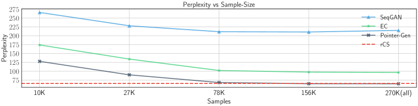
Figure 3.3: Results of perplexity (PPL) on different numbers of generated samples. The graph shows that Pointer-Gen attains a close performance to the real training data, and outperforms SeqGAN and EC.

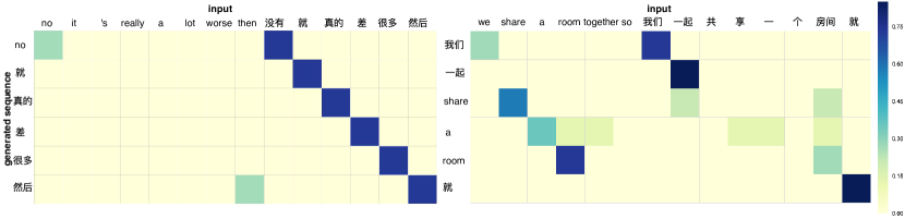
Figure 3.4: The visualization of pointer-generator attention weights on input words in each time-step during the inference time. The y-axis indicates the generated sequence, and the x-axis indicates the word input. In this figure, we show the code-switching points.

Model Interpretability

We can interpret a Pointer-Gen model by extracting its attention matrices and then analyzing the activation scores. We show the visualization of the attention weights in Figure 3.4. The square in the heatmap corresponds to the attention score of an input word. In each time-step, the attention scores are used to select words to be generated. As we can observe in the figure, in some cases, our model attends to words that are translations of each other, for example, the words (“no”,“没有”), (“then”,“然后”) , (“we”,“我们”), (“share”, “一起”), and (“room”,“房间”). This indicates the model can identify code-switching points, word alignments, and translations without being given any explicit information.

3.4 Short Summary

In this chapter, we propose two methods for generating synthetic code-switched sentences using EC and Pointer-Gen. The former method alleviates the dependency on syntactic parsers that can be applied to other language pairs, and the latter method learns how to copy words from parallel corpora. Interestingly, Pointer-Gen also captures code-switching points by attending to input words and aligning the parallel words, without requiring any word alignments or constituency parsers. More importantly, it can be effectively used for languages that are syntactically different, such as English and Mandarin. Our language model trained using Pointer-Gen outperforms the EC theory-based models and SeqGAN model.

Chapter 4 Syntax-Aware Multi-Task Learning for Code-Switched Language Modeling

LM using only word lexicons is not adequate to learn the complexity of code-switching patterns, especially in a low-resource setting. In the linguistic world, code-switching patterns can be found by observing the syntactic features that are useful information to identify code-switch points, as they are not produced randomly. Poplack [30] shows that there are higher proportions of certain types of switches in the presence of syntactic features. Therefore, we conjecture that the syntactic features are highly correlated to the code-switching triggers.

In this chapter, we propose a multi-task learning framework for the code-switching LM task, which is able to leverage syntactic features such as language information and POS tags [116]. Using syntactic features allows the model to learn shared grammatical information that constrains the next word prediction. The main contribution of this work is two-fold. First, a multi-task learning model is proposed to jointly learn the LM task and POS sequence tagging task on code-switched utterances. Second, we incorporate language information into POS tags to create bilingual tags — The tags distinguish between Chinese and English. The POS tag features are shared with the language model and enrich the features to learn better where to switch.

4.1 Model Description

The proposed multi-task learning consists of two NLP tasks: LM and POS sequence tagging. Figure 4.1 illustrates our multi-task learning extension to the recurrent language model. We use LSTM [48] in our model instead of the standard RNN. The LM task is a standard next word prediction, and the POS tagging task is to predict the next POS tag. The POS tagging task shares the POS tag vector and the hidden states to the LM task, but it does not receive any information from the other loss. Let $w_{t}$ be the word lexicon in the document and $p_{t}$ be the POS tag of the corresponding $w_{t}$ at index $t$. They are mapped into embedding matrices to get their $d$-dimensional vector representations $x_{t}^{w}$ and $x_{t}^{p}$. The input embedding weights are tied with the output weights. We concatenate $x_{t}^{w}$ and $x_{t}^{p}$ as the input of the $\textnormal{LSTM}_{lm}$. The information from the POS tag sequence is shared with the language model through this step:

$$u_{t}=\textnormal{LSTM}_{lm}(x_{t}^{w}\oplus x_{t}^{p},u_{t-1}),$$

$$v_{t}=\textnormal{LSTM}_{pt}(x_{t}^{p},v_{t-1}),$$

where $\oplus$ denotes the concatenation operator, and $u_{t}$ and $v_{t}$ are the final hidden states of $\textnormal{LSTM}_{lm}$ and $\textnormal{LSTM}_{pt}$ respectively. $u_{t}$ and $v_{t}$, the hidden states from both LSTMs, are then summed before predicting the next word. Then, we project the vector to the vocabulary space by multiplying it with learned parameters $W_{lm}^{O}$ and bias $b_{lm}$:

$$z_{t} =u_{t}+v_{t},$$ (4.1)

$$y_{t} =W_{lm}^{O}(z_{t})+b_{lm},$$ (4.2)

$$y_{t} =\frac{e^{y_{t}}}{\sum_{j=1}^{T}e^{y_{j}}}\textnormal{, where }j=1\textnormal{, .., }T.$$ (4.3)

For the POS tagging task, the model also learns a learned weight $W_{pt}^{O}$ to project vector $v$ to the POS label distribution $s$ as follows:

$$s_{t} =W_{pt}^{O}(v_{t})+b_{pt},$$ (4.4)

$$s_{t} =\frac{e^{s_{t}}}{\sum_{j=1}^{T}e^{s_{j}}}\textnormal{, where }j=1\textnormal{, .., }T.$$ (4.5)

The word distribution of the next word $y_{t}$ is normalized using the softmax function. The model uses cross-entropy losses as error functions $\mathcal{L}_{lm}$ and $\mathcal{L}_{pt}$ for the LM task and POS tagging task, respectively. We optimize the multi-objective losses using the Back Propagation algorithm, and we perform a weighted linear sum of the losses for each individual task:

$$\mathcal{L}_{total}=p\mathcal{L}_{lm}+(1-p)\mathcal{L}_{pt},$$ (4.6)

where $p$ is the weight of the loss in training.

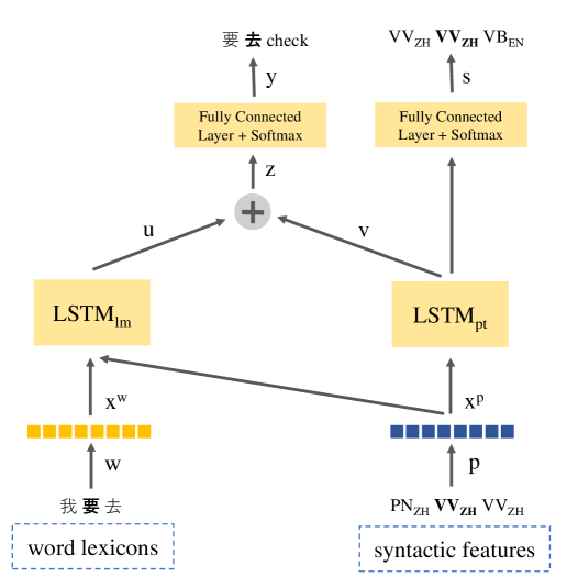
Figure 4.1: Multi-task learning framework.

4.2 Experimental Setup

4.2.1 Dataset

SEAME (South East Asia Mandarin-English), a conversational Mandarin-English code-switching speech corpus, consists of spontaneously spoken interviews and conversations [112]. Our dataset (LDC2015S04) is the most up-to-date version of the Linguistic Data Consortium (LDC) database. However, the statistics are not identical to those from Lyu et al. [117]. The corpus consists of two phases. In Phase I, only selected audio segments were transcribed, while in Phase II, most of the audio segments were transcribed. For each language island, a phrase within the same language, we extract POS tags iteratively using the Chinese and English Penn Tree Bank Parser [118, 119]. There are 31 English POS tags and 34 Chinese POS tags. Chinese words are distinguishable from English words since they have a different encoding. We add language information to the POS tag label to discriminate POS tags between the two languages. For our pre-processing steps, we tokenize English and Chinese words using the Stanford NLP toolkit [113]. Second, all hesitations and punctuation are removed except apostrophes, for example, “let’s” and “it’s.” Table 4.1 and Table 3.1 show the statistics of the SEAME Phase I and II corpora. Table 4.2 shows the most common trigger POS tags for the Phase II corpus.

Table 4.1: Data statistics in SEAME Phase I.

	Train set	Dev set	Test set
# Speakers	139	8	8
# Utterances	45,916	1,938	1,228
# Tokens	762K	31K	17K
Avg. segments length	3.67	3.68	3.18
Avg. switches	3.60	3.47	3.67

Table 4.2: Code-switching trigger words in SEAME Phase II.

POS Tag	Freq	POS Tag	Freq
$\textnormal{VV}_{ZH}$	107,133	$\textnormal{NN}_{EN}$	31,031
$\textnormal{AD}_{ZH}$	97,681	$\textnormal{RB}_{EN}$	12,498
$\textnormal{PN}_{ZH}$	92,117	$\textnormal{NNP}_{EN}$	11,734
$\textnormal{NN}_{ZH}$	45,088	$\textnormal{JJ}_{EN}$	5,040
$\textnormal{VA}_{ZH}$	27,442	$\textnormal{IN}_{EN}$	4,801
$\textnormal{CD}_{ZH}$	20,158	$\textnormal{VB}_{EN}$	4,703

4.2.2 Training

We train our LSTM models with different hidden sizes [200, 500]. All LSTMs have two layers and are unrolled for 35 steps. The embedding size is equal to the LSTM hidden size. A dropout regularization [120] is applied to the word embedding vector and POS tag embedding vector, and to the recurrent output [121] with values between [0.2, 0.4]. We use a batch size of 20 in training. An end of sentence (EOS) tag is used to separate every sentence. We use SGD and start with a learning rate of 20, and if there is no improvement during the evaluation, we reduce the learning rate by a factor of 0.75. The gradient is clipped to a maximum of 0.25. For multi-task learning, we use different weight loss hyper-parameters $p$ in the range of [0.25, 0.5, 0.75]. We tune our model with the development set and evaluate our best model using the test set, taking PPL as the final evaluation metric, which is calculated by taking the exponential of the error in the negative log-form:

$$\textnormal{PPL}(w)=P(\mathbf{w}_{1},\mathbf{w}_{2},...,\mathbf{x}_{N})^{-\frac{1}{N}}=\sqrt[N]{\frac{1}{P(\mathbf{w}_{1},\mathbf{w}_{2},...,\mathbf{w}_{N})}}.$$ (4.7)

4.2.3 Evaluation

We evaluate our proposed method on both SEAME Phase I and Phase II. We compare our method with existing baselines only on SEAME Phase I, since all of those models were only evaluated on the Phase I dataset. The baselines are as follows:

RNNLM

The baseline model trained using RNNLM [122].

wFLM

The factored language model proposed by Adel et al. [65] using FLM open class clusters, brown clusters, part-of-speech and the trigram language model.

FI + OF

The model from Adel et al. [63] that uses a factorized RNNLM with POS as input and is trained with a multi-task objective to predict the next word and language.

RNNLM + FLM

The model from Adel et al. [69] that combines FLM with RNNLM by language model interpolation.

4.3 Results and Discussion

Table 4.3 and Table 4.4 show the results of multi-task learning with different values of the hyper-parameter $p$. We observe that the multi-task model with $p=0.25$ achieves the best performance. We compare our multi-task learning model against the RNNLM and LSTM baselines. The baselines correspond to RNNs that are trained with word lexicons. Table 4.5 and Table 4.6 present the overall results from the different models. The multi-task model performs better than the LSTM baseline by 9.7% PPL in Phase I and 7.4% PPL in Phase II. The performance of our model in Phase II is also better than the RNNLM (8.9%) and far better than the one presented in [69] in Phase I. Moreover, the results show that adding a shared POS tag representation to $\textnormal{LSTM}_{lm}$ does not hurt the performance of the LM task. This implies that the syntactic information helps the model to better predict the next word in the sequence. To further verify this hypothesis, we conduct two analyses by visualizing our prediction examples, as shown in Figure 4.2.

Table 4.3: Multi-task results with different weighted loss hyper-parameters in SEAME Phase I.

Hidden size	$p$	PPL Dev	PPL Test
200	0.25	180.90	178.18
	0.50	182.60	178.75
	0.75	180.90	178.18
500	0.25	173.55	174.96
	0.50	175.23	173.89
	0.75	185.83	178.49

Table 4.4: Multi-task results with different weighted loss hyper-parameters in SEAME Phase II.

Hidden size	$p$	PPL Dev	PPL Test
200	0.25	149.68	149.84
	0.5	150.92	152.38
	0.75	150.32	151.22
500	0.25	141.86	141.71
	0.5	144.18	144.27
	0.75	145.08	144.85

Table 4.5: Language model results in SEAME Phase I

Model	PPL Dev	PPL Test
RNNLM [63]	246.60	287.88
wFLM [65]	238.86	245.40
FI + OF [63]	219.85	239.21
RNNLM + FLM [69]	177.79	192.08
LSTM	190.33	185.91
+ syntactic features	178.51	176.57
Multi-task	173.55	174.96

Table 4.6: Language model results in SEAME Phase II

Model	PPL Dev	PPL Test
RNNLM [63]	178.35	171.27
LSTM	150.65	153.06
+ syntactic features	147.44	148.38
Multi-task	141.86	141.71

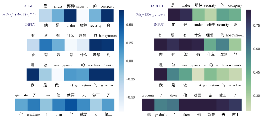
Figure 4.2: Prediction examples in Phase II. Left: Each square shows the target word’s log probability improvement with the multi-task model compared to the LSTM model (darker color is better). Right: Each square shows the probability that the next POS tag is Chinese (darker color represents higher probability).

To measure the target word’s log probability with the multi-task model compared to the standard LSTM model, we calculate the log probability difference between the two models. According to Figure 4.2, in most cases, the multi-task model improves the prediction of the monolingual segments, and particularly at code-switching points, such as “under”, “security”, “generation”, “then”, “graduate”, “他”, and “的”. It also shows that the multi-task model is more precise in learning where to switch the language. Meanwhile, Table 4.2 shows the relative frequency of the trigger POS tag. The word “then” belongs to $\textnormal{RB}_{EN}$, which is one of the most common trigger words in the list. Furthermore, the target word prediction is significantly improved in most of the trigger words. We report the probability that the next produced POS tag is Chinese. It is shown that the words “then”, “security”, “了”, “那种”, “做”, and “的” tend to switch the language context within the utterance. However, it is very hard to predict all the cases correctly. This may be due to the fact that without any switching, the model still creates a correct sentence.

4.4 Short Summary

In this chapter, we propose a multi-task learning approach for code-switched LM that leverages syntactic information. The multi-task learning models achieve the best performance and outperform the LSTM baseline with 9.7% and 7.4% improvement in PPL for the Phase I and Phase II SEAME corpus, respectively. This implies that by training two different NLP tasks together, the models can correctly learn the correlation between them. Indeed, the syntactic information helps the model to be aware of code-switching points, and it improves the performance over the LM. Finally, we conclude that multi-task learning has good potential for code-switching LM research.

Chapter 5 Multi-Task Learning for End-to-End Code-Switched Speech Recognition

ASR is the first step in the pipeline of a conversational agent and positively affects the response of the overall system. Any errors made by the ASR system will propagate through other modules and lead to failures in the conversation. Thus, robust ASR systems are crucial. Since code-switched data are limited, transfer learning approaches have become very important for domain adaptation. Li and Fung [24] proposed to first train an English-Chinese bilingual model using monolingual datasets, and then fine-tune the model using a small number of code-switched data. Then, they also augment the synthetic code-mixed speech with linguistic constraints to improve the language model re-scoring.

In this chapter, we focus on applying an end-to-end neural-based approach without using any LID. Since errors in LID affect the prediction of the model, we aim to remove dependency on the language. And since code-switching is considered low-resource, we take a transfer learning approach to leverage monolingual resources for the code-switching domain. We examine different training approaches to train code-switching end-to-end speech recognition models, and explore transfer learning methods to improve code-switching speech recognition to address the low-resource issue. Commonly, high-resource monolingual speech data are used to improve the generalization ability of code-switching models as an adaptation method. Intuitively, this approach may help the model recognize individual languages, which can eventually distinguish phones from different languages. We will introduce two training strategies: multi-task training and meta-transfer learning.

5.1 Model Description

5.1.1 Architecture

We build our speech recognition model on a transformer-based encoder-decoder to learn to predict graphemes from the speech input. Our model extracts audio inputs with a learnable feature extractor module to generate input embeddings. The model is illustrated in Figure 5.1. The encoder uses input embeddings generated from the feature extractor module. The decoder receives the encoder outputs and applies multi-head attention to its input to finally calculates the logits of the outputs. To generate the probability of the outputs, we compute the softmax function of the logits. We apply a mask in the attention layer to avoid any information flow from future tokens, and train our model by optimizing the next-step prediction on the previous characters and maximizing the log probability:

$$\max_{\theta}\sum_{i}\log{P(y_{i}|x,y^{\prime}_{<i};\theta)},$$ (5.1)

where $x$ is the character inputs, $y_{i}$ is the next predicted character, and $y^{\prime}_{<i}$ is the previous groundtruth characters.

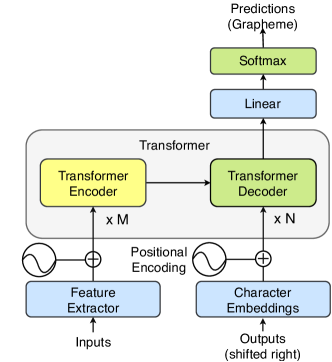
Figure 5.1: Transformer ASR model architecture.

5.1.2 Inference

To further improve the prediction, we incorporate Pointer-Gen LM [28] in the beam search process to select the best sub-sequence scored using the softmax probability of the characters. We define $P(Y)$ as the probability of the predicted sentence, and add the Pointer-Gen LM $P_{lm}(Y)$ to rescore the predictions. We also include word count wc(Y) to avoid generating very short sentences. $P(Y)$ is calculated as follows:

$$\alpha\sum_{i}\log{P(y_{i}|x,\hat{y}_{<i};\theta)}+\beta P_{lm}(\hat{y}_{<i})+\gamma\sqrt{wc(\hat{y}_{<i})},$$ (5.2)

where $\alpha$ is the parameter to control the decoding probability from the decoder, $\beta$ is the parameter to control the language model probability, and $\gamma$ is the parameter to control the effect of the word count $wc(\hat{y}_{<i})$.

5.2 Training Strategies

5.2.1 Standard Multi-Task Training

To learn information from several datasets, we can jointly train all of them together [123]. This training strategy enables the model to generalize well on all tasks. Figure 5.3 (a) shows the intuition of how the trained parameter $\theta$ is in the center of all tasks. The algorithm is relatively simple as it draws the same number of samples from each task and trains them together in the gradient update. By learning in this way, the model can capture information from all sources, which is useful in the case of code-switching because there is overlapping information between code-switching and monolingual sources.

5.2.2 Meta-Transfer Learning

We propose our Meta-Transfer Learning by first introducing Model-Agnostic Meta-Learning (MAML).

Model-Agnostic Meta-Learning

MAML [124, 125] learns to quickly adapt to a new task from a number of different tasks using a gradient descent procedure, as shown in Figure 5.2.

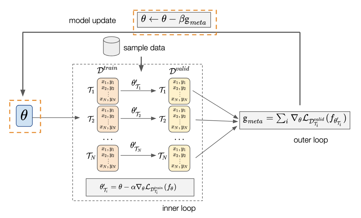
Figure 5.2: Model-Agnostic Meta-Learning (MAML) training mechanism.

We apply MAML to effectively learn from a set of accents and quickly adapt to a new accent in the few-shot setting. We denote our transformer ASR as $f_{\theta}$ parameterized by $\theta$. Our dataset consists of a set of accents $\mathcal{A}=\{A_{1},A_{2},\cdots,A_{n}\}$, and for each accent $i$, we split the data into $A_{i}^{tra}$ and $A_{i}^{val}$. Then we update $\theta$ into $\theta^{\prime}$ by computing gradient descent updates on $A_{i}^{tra}$:

$$\theta_{i}^{\prime}=\theta-\alpha\nabla_{\theta}{\mathcal{L}_{A_{i}^{tra}}(f_{\theta})},$$ (5.3)

where $\alpha$ is the fast adaptation learning rate. During the training, the model parameters are trained to optimize the performance of the adapted model $f(\theta_{i}^{\prime})$ on unseen $A_{i}^{val}$. The meta-objective is defined as follows:

$$\min_{\theta}\sum_{A_{i}\sim p(\mathcal{A})}\mathcal{L}_{A_{i}^{val}}(f_{\theta_{i}^{\prime}})=\sum_{A_{i}\sim p(\mathcal{A})}\mathcal{L}_{A_{i}^{val}}(f_{\theta-\alpha\nabla_{\theta}\mathcal{L}_{A_{i}^{tra}}(f_{\theta})}),$$ (5.4)

where $\mathcal{L}_{A_{i}^{val}}(f_{\theta_{i}^{\prime}})$ is the loss evaluated on $A_{i}^{val}$. We collect the loss $\mathcal{L}_{A_{i}^{val}}(f_{\theta_{i}^{\prime}})$ from a batch of accents and perform the meta-optimization as follows:

$$\theta\leftarrow\theta-\beta{\sum_{A_{i}\sim p(\mathcal{A})}\nabla_{\theta}\mathcal{L}_{A_{i}^{val}}(f_{\theta_{i}^{\prime}})},$$ (5.5)

where $\beta$ is the meta step size and $f_{\theta_{i}^{\prime}}$ is the adapted network on accent $A_{i}$. The meta-gradient update step is performed to achieve a good initialization for our model. Then we can optimize our model with a small number of samples on target accents in the fine-tuning step. In this chapter, we use first-order approximation MAML as in [126] and [127]. Thus, Equation 5.5 is reformulated as

$$\theta\leftarrow\theta-\beta{\sum_{A_{i}\sim p(\mathcal{A})}\nabla_{\theta_{i}^{\prime}}\mathcal{L}_{A_{i}^{val}}(f_{\theta_{i}^{\prime}})}.$$ (5.6)

Our Approach

Our approach extends the meta-learning paradigm to adapt knowledge learned from source domains to a specific target domain. Compared to MAML, we only assign code-switching data in $\mathcal{D}^{val}$ and take both monolingual and code-switching data in $\mathcal{D}^{train}$. So, the model is only tuned from the gradients evaluated from code-switching data. This approach captures useful information from multiple resources for the target domain and updates the model accordingly. Figure 5.3 presents the general idea of our Meta-Transfer Learning. Its goal is not to generalize to all tasks but to focus on acquiring crucial knowledge to transfer from monolingual resources to the code-switching domain. As shown in Algorithm 1, for each adaptation step on $\mathcal{T}_{i}$, we compute updated parameters $\theta_{i}^{\prime}$ via SGD as follows:

$$\theta_{i}^{\prime}=\theta-\alpha\nabla_{\theta}\mathcal{L}_{\mathcal{D}_{i}^{tra}}(f_{\theta}),$$ (5.7)

where $\alpha$ is a learning hyper-parameter of the inner optimization. Then, a cross-entropy loss $\mathcal{L}_{D_{i}}$ is calculated from a learned model upon the generated text given the audio inputs on the target domain $j$:

$$\mathcal{L}_{D_{i}}=-\sum_{\mathcal{D}^{val}\sim\mathscr{D}_{tgt}}\log p(y_{t}|x_{t};\theta^{\prime}_{i}).$$ (5.8)

We define the objective as follows:

$$\min_{\theta}\sum_{\mathcal{D}_{i}^{tra},\mathcal{D}^{val}}\mathcal{L}_{\mathcal{D}^{val}}(f_{\theta_{i}^{\prime}})=$$ (5.9)

$$\sum_{\mathcal{D}_{i}^{tra},\mathcal{D}^{val}}\mathcal{L}_{\mathcal{D}^{val}}(f_{\theta-\alpha\nabla_{\theta}\mathcal{L}_{D_{i}^{tra}}(f_{\theta})}),$$ (5.10)

where $\mathcal{D}_{i}^{tra}\sim(\mathscr{D}_{src},\mathscr{D}_{tgt})$ and $\mathcal{D}^{val}\sim\mathscr{D}_{tgt}$. We minimize the loss of the $f_{\theta^{\prime}_{i}}$ upon $\mathcal{D}^{val}$. Then, we apply gradient descent on the meta-model parameter $\theta$ with a $\beta$ meta-learning rate.

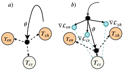
Figure 5.3: Illustration of (a) joint training and (b) Meta-Transfer Learning. The solid lines show the optimization path. The orange circles represent the monolingual source language, and the white circles represent the code-switching target language. The lower black circle in (b) is closer to $T_{cs}$ than that in (a).

Algorithm 1 Meta-Transfer Learning

Require: $\mathscr{D}_{src}$, $\mathscr{D}_{tgt}$
Require: $\alpha,\beta$: step size hyper-parameters

1:Randomly initialize $\theta$

2:while not done do

3:     Sample batch data $\mathcal{D}^{tra}_{i}\sim(\mathscr{D}_{src},\mathscr{D}_{tgt})$, $\mathcal{D}^{val}\sim\mathscr{D}_{tgt}$

4:     for all $\mathcal{D}^{tra}_{i}$ do

5:         Evaluate $\nabla_{\theta}\mathcal{L}_{\mathcal{D}^{tra}_{i}}(f_{\theta})$ using $\mathcal{D}^{tra}_{i}$

6:         Compute adapted parameters with gradient descent: .. $\theta^{\prime}_{i}=\theta-\alpha\nabla_{\theta}\mathcal{L}_{\mathcal{D}^{tra}_{i}}(f_{\theta})$

7:     end for

8:     $\theta\leftarrow\theta-\beta\sum_{i}\nabla_{\theta}\mathcal{L}_{\mathcal{D}^{val}}\left(f_{\theta_{i}^{\prime}}\right)$

9:end while

5.3 Experiments and Results

5.3.1 Datasets

We use SEAME Phase II, a conversational English-Mandarin Chinese code-switching speech corpus that consists of spontaneously spoken interviews and conversations [112]. The details are depicted in Table 3.1. For the monolingual speech datasets, we use HKUST [114] as the monolingual Chinese dataset and Common Voice v1 as the monolingual English dataset. We use 16 kHz audio inputs and up-sample the HKUST data from 8 to 16 kHz.

5.3.2 Experiment Settings

Our transformer model consists of two encoder and four decoder layers with a hidden size of 512, an embedding size of 512, a key dimension of 64, and a value dimension of 64. The input of all experiments is a spectrogram, computed with a 20 ms window, and shifted every 10 ms. Our label set has 3765 characters and includes all English and Chinese characters from the corpora, spaces, and apostrophes. We optimize our model using Adam and start the training with a learning rate of 1e-4. We fine-tune our model using SGD with a learning rate of 1e-5, and apply an early stop on the validation set. We choose $\alpha=1$, $\beta=0.1$, and $\gamma=0.1$. We draw the sample of the batch randomly with a uniform distribution every iteration. We define cs as the code-switching dataset, en as the English dataset, and zh as the Chinese dataset. We conduct experiments with the following approaches: (a) only cs, (b) joint training on en + zh, (c) joint training on cs + en + zh, and (d) Meta-Transfer Learning. Then, we fine-tune the trained models (b), (c), and (d) on cs, and we apply language model rescoring on our best model. We evaluate our model using beam search with a beam width of 5 and maximum sequence length of 300. The quality of our model is measured using CER.

Multi-task Learning End-to-end ASR

We convert the inputs into normalized frame-wise spectrograms from 16-kHz audio. Our transformer model consists of two encoder and decoder layers. The Adam optimizer and Noam warmup are used for training with an initial learning rate of 1e-4. The model has a hidden size of 1024, a key dimension of 64, and a value dimension of 64. The training data are randomly shuffled every epoch. Our character set is the concatenation of English letters, Chinese characters found in the corpus, spaces, and apostrophes. In the multilingual ASR pre-training, we train the model for 18 epochs. Since the sizes of the datasets are different, we over-sample the smaller dataset. The fine-tuning step takes place after the pretraining using code-switching data. In the inference time, we explore the hypothesis using beam search with a beam width of 8 and a batch size of 1.

Character Error Rate (CER)

For our ASR, we compute the overall CER and also show the individual CERs for Mandarin Chinese (zh) and English (en). The metric calculates the distance of two sequences as the Levenshtein Distance.

Table 5.1: Results of the evaluation on CER. Lower CER is better. Meta-Transfer Learning is more effective in transferring information from the monolingual datasets.

	$\downarrow$ CER
Winata et al. [28]	32.76%
+ Pointer-Gen LM	31.07%
Only cs	34.51%
Joint Training (en + zh)	98.29%
+ Fine-tuning	31.22%
Joint Training (en + zh + cs)	32.87%
+ Fine-tuning	31.90%
Meta-Transfer Learning	30.30%
+ Fine-tuning	29.99%
+ Pointer-Gen LM	29.30%

5.3.3 Results

The results are shown in Table 5.1. Generally, adding monolingual data en and zh as the training data is effective to reduce the error rate. There is a significant margin between only cs and joint training (1.64%) or meta-transfer learning (4.21%). According to the experiment results, meta-transfer learning consistently outperforms the joint-training approaches, which shows its effectiveness in language adaptation. The fine-tuning approach helps to improve the performance of the trained models, especially on the jointly trained (en + zh). We observe that joint training on (en + zh) without fine-tuning cannot predict mixed-language speech, while joint training on en + zh + cs is able to recognize it. However, according to Table 5.2, adding a fine-tuning step badly affects the previously learned knowledge (e.g., en: 11.84%$\rightarrow$63.85%, zh: 31.30%$\rightarrow$78.07%). Interestingly, the model trained with Meta-Transfer Learning does not suffer catastrophic forgetting, even without focusing the loss objective to learn both monolingual languages. As expected, joint training on en + zh + cs achieves decent performance on all tasks, but it does not optimally improve cs.

The language model rescoring using Pointer-Gen LM improves the performance of the Meta-Transfer Learning model by choosing more precise code-switching sentences during beam search. Pointer-Gen LM improves the performance of the model and outperforms the model trained only in cs by 5.21% and the previous state-of-the-art by 1.77%.

Table 5.2: Performance on monolingual English (en) and Chinese (zh) in terms of CER. $\Delta$ CER denotes the improvement on cs test set relative to the baseline (Only cs) model.

	$\uparrow$ $\Delta$ CER	$\downarrow$ en	$\downarrow$ zh
Only cs	0	66.71%	99.66%
Joint Training (en + zh)	-63.78%	11.84%	31.30%
+ Fine-tuning	3.29%	63.85%	78.07%
Joint Training (en + zh + cs)	1.64%	13.88%	30.46%
+ Fine-tuning	2.61%	57.56%	76.20%
Meta-Transfer Learning	4.21%	16.22%	31.39%

Convergence Rate

Figure 5.4 depicts the dynamics of the validation loss per iteration on cs, en, and zh. As we can see from the figure, Meta-Transfer Learning is able to converge faster than joint training, and ends in the lowest validation loss. For the validation losses on en and zh, both joint training (en + zh + cs) and Meta-Transfer Learning achieve similar loss in the same iteration. This shows that Meta-Transfer Learning is not only optimized for the code-switching domain, but also preserves the generalization ability to monolingual domains, as depicted in Table 5.2.

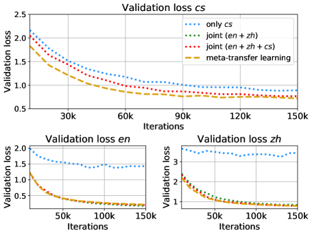
Figure 5.4: Validation loss per iteration. Top: validation loss on cs data, (joint ($en$ + $zh$) is omitted because it is higher than the range), bottom left: validation loss on $en$ data, bottom right: validation loss on $zh$ data.

Language Model

Table 5.3: Results on the language modeling task in PPL.

Model	valid	test
Only cs	72.89	65.71
Joint Training (en + zh + cs)	70.99	63.73
+ Fine-tuning	69.66	62.73
Meta-Transfer Learning (en + zh + cs)	68.83	62.14
+ Fine-tuning	68.71	61.97

We further evaluate our meta-transfer learning approach on a language model task. We simply take the transcription of the same datasets and build a two-layer LSTM-based language model following the model configuration in Winata et al. [28]. To further improve the performance, we apply fine-tuning with an SGD optimizer by using a learning rate of 1.0, and decay the learning rate by 0.25x for every epoch without any improvement in the validation performance. To prevent the model from over-fitting, we add an early stop of 5 epochs. As shown in Table 5.3, the Meta-Transfer Learning approach outperforms the joint-training approach. We find a similar trend for the language model task results on the speech recognition task, where Meta-Transfer Learning without additional fine-tuning performs better than joint training with fine-tuning. Compared to our baseline model (Only cs), Meta-Transfer Learning is able to reduce the test set PPL by 3.57 points (65.71 $\rightarrow$ 62.14), and the post fine-tuning step reduces the test set PPL even further, from 62.14 to 61.97.

5.4 Short Summary

In this chapter, we propose a novel multi-task learning method, Meta-Transfer Learning, to transfer learn on a code-switched speech recognition system in a low-resource setting by judiciously extracting information from high-resource monolingual datasets. Our model recognizes individual languages and transfers them to better recognize mixed-language speech by conditioning the optimization objective to the code-switching domain. Experimental results show that our model outperforms existing baselines in terms of error rate, and it is also faster to converge.

Chapter 6 Representation Learning for Code-Switched Sequence Labeling

Sequence labeling, such as POS tagging and NER, is a key module for NLU systems. This module is important in understanding the semantics of the word sequence. Training a code-switched model is very challenging because monolingual taggers erroneously tag tokens, and the semantics of a word may be different between languages. The other problem in code-switched sequence labeling is how to represent embeddings on code-switched sequences, and many existing code-switched datasets are not annotated with language information. In code-switching, there is ambiguity in the semantics since the same words may be found in two or more languages. The standard approach in working on code-switching is to first predict the language and then take a corresponding embedding according to the predicted language. However, this may not be accurate, when the same word appears in the code-switched languages. For instance, the word “cola” can be associated with a product or is the word for “queue” in Spanish. Thus, the challenge in code-switching is learning a language-agnostic representation without any information about the language of the word.

Learning representation for code-switching has become a prominent area of research in NLP applications to support a greater variety of language speakers. However, despite the enormous number of studies in multilingual NLP, only very few focus on code-switching. Recently, contextualized language models, such as mBERT [94] and XLM-R [128] have been proposed to tackle monolingual and cross-lingual tasks in NLU benchmarks [129, 130, 100, 96, 131], and they have achieved impressive performance. The effectiveness and efficiency of these multilingual language models on code-switching tasks, however, remains unknown. Thus, in this chapter, we will propose an effective approach to improve the representation of code-switching sentences that is efficient enough to be applied in practical scenarios.

In the following sections, we will present three key contributions:

• We introduce a method to train bilingual character embeddings using a BiLSTM for learning representations on code-switched data to show the effectiveness of combining words and characters. This method is very effective to address the OOV issue.

• We propose multilingual meta-embedding approaches for learning representations on code-switching data using neural-based models to combine embeddings from different languages without LID.

• We also present a comprehensive study on the effectiveness of multilingual models on a variety of code-switching NLU tasks to analyze the practicality of each model in terms of performance, speed, and number of parameters. We further analyze the memory footprint required by each model over different sequence lengths in a GPU. Thus, we are able to understand which model to choose in a practical scenario.

6.1 Bilingual Character Embeddings

6.1.1 Model Architecture

Combining lexical structures (word, subword, and characters) is a common technique to improve representations by leveraging lexical composition. Lample et al. [132] proposed character-based word representations learned from a supervised corpus and unsupervised word representations learned from unannotated corpora. In the context of code-switching, we have explored a mixture of word and character embeddings [19]. Figure 6.1 shows the combination of word embeddings and embeddings generated from a bilingual character RNN. We use a word embedding taken from either $L_{1}$ or $L_{2}$.

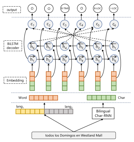
Figure 6.1: Word and character embeddings for sequence labeling.

Consider a sequence of word embeddings $\textbf{x}={(x_{1},x_{2},...,x_{M})}$ and character embeddings $\textbf{a}={(a_{1},a_{2},...,a_{N})}$, where $M$ is the length of the word sequence and $N$ is the length of the character sequence. The word embeddings are fixed. Then, we concatenate both word and character vectors to get a richer word representation $u_{t}$. Afterwards, we pass the vectors to a BiLSTM.

$$u_{t} =x_{t}\oplus a_{t},$$ (6.1)

$$\overrightarrow{h_{t}} =\overrightarrow{\textnormal{LSTM}}(u_{t},\overrightarrow{h_{t-1}}),$$ (6.2)

$$\overleftarrow{h_{t}} =\overleftarrow{\textnormal{LSTM}}(u_{t},\overleftarrow{h_{t-1}}),$$ (6.3)

$$c_{t} =\overrightarrow{h_{t}}\oplus\overleftarrow{h_{t}},$$ (6.4)

where $\oplus$ denotes the concatenation operator. Dropout is applied to the recurrent layer. At each time step we make a prediction for the entity of the current token. The softmax function is used to calculate the probability distribution of all possible named-entity tags:

$$y_{t}=\frac{e^{c_{t}}}{\sum_{j=1}^{T}e^{c_{j}}}\textnormal{, where }j=1\textnormal{, .., T},$$ (6.5)

where $\textnormal{y}_{t}$ is the probability distribution of tags at word $t$ and T is the maximum time step. Since there is a variable number of sequence lengths, we pad the sequence and apply a mask when calculating the cross-entropy loss function. Our model does not use a gazetteer or knowledge-based information, and it can be easily adapted to another language pair.

Bilingual Char-RNN

We use an RNN to represent a word with character-level information [132]. Figure 6.2 shows the model architecture of our Char-RNN. The inputs are characters extracted from a word, and every character is embedded with a $d$-dimension vector. Then, we use this as the input for a BiLSTM as a character encoder, wherein, at every time step, a character is input to the network.

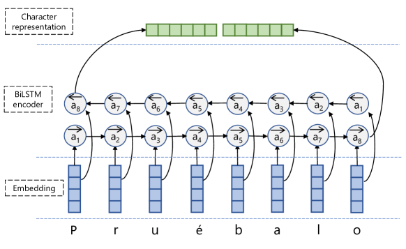
Figure 6.2: Bilingual Char-RNN architecture.

Pre-processing

In this section, we describe word-level and character-level features used in our model. The pre-processing is done before we start training the model. Words are encoded into a continuous representation. The vocabulary is built from training data. We apply preprocessing steps since our data are noisy and come from Twitter. There are many spelling mistakes, irregular word usages and repeated characters. To create the shared vocabulary, we concatenate $L_{1}$ and $L_{2}$ word vectors. For pre-processing, we propose the following steps:

1. Token replacement: Replace user hashtags (#user) and mentions (@user) with “USR”, and URL (https://domain.com) with “URL”.

2. Token normalization: Concatenate $L_{1}$ and $L_{2}$ FastText word vector vocabulary. Normalize OOV words by sequentially checking if the word exists after applying the following changes:

   1. Capitalize the first character

   2. Lowercase the word

   3. Do (b) and remove repeated characters, such as “hellooooo” to “hello” or “lolololol” to “lol”

   4. Do steps (a) and (c) together

As shown in Table 6.3, pre-processing and transfer learning are effective in handling OOV words and the pre-processing strategies dramatically decrease the number of unknown words. We concatenate all possible characters for English and Spanish, including numbers and special characters. English and Spanish have most characters in common, but, Spanish has some additional unique characters. All cases are kept as they are.

6.1.2 Experimental Setup

Dataset

In this experiment, we use English-Spanish NER tweets data from the CALCS 2018 shared task [79]. There are nine different named-entity labels, which all use the IOB format (Inside, Outside, Beginning), where every token is labeled with a B-label in the beginning, followed by an I-label if it is inside a named entity, or O otherwise. For example “Kendrick Lamar” is represented as B-PER I-PER. Table 6.2 and Table 6.3 show the statistics of the dataset.

Table 6.1: OOV word rates on ENG-SPA dataset before and after pre-processing.

	Train		Dev		Test
	All	Entity	All	Entity	All
Corpus	-	-	18.91%	31.84%	49.39%
FastText (eng) [90]	62.62%	16.76%	19.12%	3.91%	54.59%
+ FastText (spa) [91]	49.76%	12.38%	11.98%	3.91%	39.45%
+ token replacement	12.43%	12.35%	7.18%	3.91%	9.60%
+ token normalization	7.94%	8.38%	5.01%	1.67%	6.08%

Table 6.2: Data statistics for ENG-SPA tweets.

	Train	Dev	Test
# Words	616,069	9,583	183,011

Table 6.3: Entity statistics for ENG-SPA tweets

Entities	Train	Dev
# Person	4701	75
# Location	2810	10
# Product	1369	16
# Title	824	22
# Organization	811	9
# Group	718	4
# Time	577	6
# Event	232	4
# Other	324	6

“Person”, “Location”, and “Product” are the most frequent entities in the dataset, and the least common are the “Time”, “Event”, and “Other” categories. The “Other” category is the least trivial among them because it is not well clustered like the others. We found an issue during the prediction where some words are labeled with O, in between B-label and I-label tags. Our solution is to insert an I-label tag if the tag is surrounded by a B-label and I-label tags with the same entity category. Another problem we found is that many I-label tags are paired with a B-label in different categories. So, we replace the B-label category tag with the corresponding I-label category tag. This step improves the results of the prediction on the development set.

Model Training

We train our LSTM models with a hidden size of 200 and use a batch size equal to 64. The sentences are sorted by length in descending order. Our embedding size is 300 for words and 150 for characters. Dropout [120] of 0.4 is applied to all LSTMs. The Adam optimizer is chosen to have an initial learning rate of 0.01. We apply time-based decay of a $\sqrt{2}$ decay rate and stop after two consecutive epochs without improvement. We tune our models with the development set and evaluate our best model with the test set using the harmonic mean F1-score metric with the script provided by Aguilar et al. [79].

6.1.3 Results and Discussion

Table 6.4 gives the results for ENG-SPA tweets, showing that adding pre-trained word vectors and character-level features improves the performance. Interestingly, our initial attempts at adding character-level features did not improve the overall performance, until we applied dropout to the Char-RNN. The performance of the model improves significantly after transfer learning with FastText word vectors, while it also reduces the number of OOV words in the development and test set. We use a subword representation from Spanish FastText [91]. However, it does not improve the results since the OOV words consist of many special characters, for example, “/IAtrevido/Provocativo”, and “Twets/wek”, and possibly create noisy vectors, while most are also not entity words.

Table 6.4: Results on ENG-SPA Dataset.

Model	Features	F1 Dev	F1 Test
BiLSTM	Word	-	53.28%
BiLSTM	Word + Char-RNN	46.96%	53.48%
BiLSTM	FastText (eng)	57.72%	59.91%
BiLSTM	FastText (eng-spa)	57.42%	60.24%
BiLSTM	+ Char-RNN	65.22%	61.96%
+ post		65.39%	62.76%

6.2 Meta-Embeddings

6.2.1 Simple Meta-Embeddings

Creating new embeddings by combining existing embeddings has been shown to be an important research direction in NLP. Bansal et al. [133] show that an ensemble of word representations outperforms single word embeddings, which implies the complementarity of different word embeddings and suggests that adding more embeddings could be a useful technique to build a better word context. Meta-embeddings aim to learn how to effectively combine pre-trained word embeddings in supervised training into a single dense representation [134, 135, 136, 137, 138]. This method is known to be effective to overcome domain and modality limitations. Given a set of $n$ embeddings $\mathbf{E}=\{E_{1},E_{2},...,E_{k},...,E_{n-1},E_{n}\}$, where each has a different embedding size $d_{k}$, there are many ways to form meta-embeddings. Figure 6.3 shows the three main architectures of meta-embeddings: concatenated, linear, and attention-based. These architectures are introduced in the following.

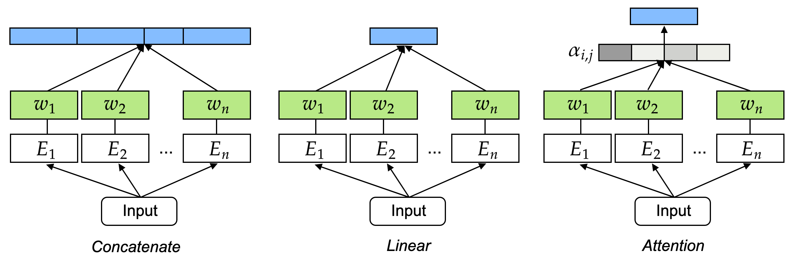
Figure 6.3: Meta-embeddings architecture.

Concatenation

A naive method to combine multiple sources of embeddings is concatenation. It is a very simple method, but it has shown good performance in semantic similarity measurement and word analogy detection, as shown by Bollegala et al. [136]. Here, we can say that it creates a higher embedding dimension and the computation is more expensive according to the number of embeddings combined. The final embeddings is

$$\mathbf{w}_{meta}=[\mathbf{w}_{1},\mathbf{w}_{2},...,\mathbf{w}_{n}].$$ (6.6)

Linear

Instead of concatenating the embeddings, we can simply sum all of them with an equal weight by assuming the embedding sizes are the same. If the embedding sizes are different, we need to project the embeddings beforehand. The final embeddings is

$$\mathbf{w}_{meta}=\sum_{i=0}^{n}{\phi(\mathbf{w}_{i})}.$$ (6.7)

Attention

We can learn a simple attention mechanism to weight embeddings from several sources, and apply the weights to embeddings. The final embeddings is

$$\mathbf{w}_{meta}=\sum_{i=0}^{n}{\alpha_{i}\phi(\mathbf{w}_{i})}.$$ (6.8)

In the context of code-switching,  Wang et al. [139] concatenate the weighted embeddings. If a word embedding is available in one language, but not in the other, the second language embeddings are initialized as a zero-vector.

6.2.2 Multilingual Meta-Embeddings

Word embedding pre-training is a well-known method to transfer knowledge from previous tasks to a target task that has fewer high-quality training data. Word embeddings are commonly used as features in supervised learning problems. We extend the idea of meta-embeddings to solve a multilingual task, and take a new perspective by combining embeddings from different languages. A word may appear in more than one language, and by taking embeddings from different language sources, we conjecture commonalities in semantics among languages.

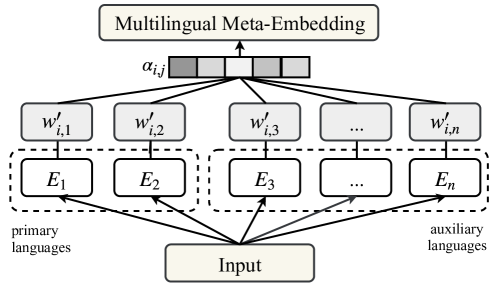
Figure 6.4: Multilingual meta-embeddings architecture.

We propose to generate a single word representation by extracting information from different pre-trained embeddings. We apply a non-linear gating function to attend to pre-trained embeddings and explore the possibility of utilizing more languages for generating multilingual meta-embeddings. We define a sentence that consists of $m$ words $\{\mathbf{x}_{j}\}_{j=1}^{m}$, and $\{\mathbf{w}_{i,j}\}_{j=1}^{n}$ word vectors from $n$ pre-trained word embeddings. We generate a multilingual vector representation for each word by taking a weighted sum of monolingual embeddings. Each embedding $\textbf{w}_{i,j}$ is projected with a fully connected layer with a non-linear scoring function $\phi$ (e.g., tanh) into a $d$-dimensional vector and an attention mechanism to calculate the attention weight $\alpha_{i,j}\in\mathbb{R}^{d}$:

$$\mathbf{w}_{i}^{MME} =\sum_{j=1}^{n}{\alpha_{i,j}\mathbf{w^{\prime}}_{i,j}},$$ (6.9)

$$\alpha_{i,j} =\frac{e^{\phi(\mathbf{w^{\prime}}_{i,j})}}{\sum_{j=1}^{n}e^{\phi(\mathbf{w^{\prime}}_{i,j}))}}.$$ (6.10)

6.2.3 Hierarchical Meta-Embeddings

Previous works have mostly focused on applying pre-trained word embeddings from each language in order to represent noisy mixed-language text, and combining them with character-level representations [140, 139, 19]. However, despite the effectiveness of such word-level approaches, they neglect the importance of subword-level characteristics shared across different languages. Such information is often hard to capture with word embeddings or randomly initialized character-level embeddings. Naturally, we can turn towards subword-level embeddings such as FastText [91] to help in this task, which would allow us to leverage the morphological structures shared across different languages. Despite their likely usefulness, little attention has been focused around using subword-level features in this task. This is partly because of the non-triviality of combining language embeddings in the subword space, which arises from the distinct segmentation into subwords for different languages. The lack of attention leads us to explore the literature of meta-embeddings [134, 135, 136, 137, 138, 141], a method to learn how to combine embeddings.

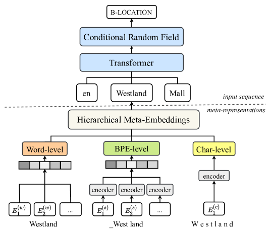
Figure 6.5: Hierarchical meta-embeddings architecture.

We propose a method to combine word, subword, and character representations to create a mixture of embeddings [142]. We generate multilingual meta-embeddings of words and subwords, and then concatenate them with character-level embeddings to generate final word representations, as shown in Figure 6.5. Let $\mathbf{w}$ be a sequence of words with $n$ elements, where $\mathbf{w}=[w_{1},\dots,w_{n}]$. Each word can be tokenized into a list of subwords $\mathbf{s}=[s_{1},\dots,s_{m}]$ and a list of characters $\mathbf{c}=[c_{1},\dots,c_{p}]$. The list of subwords $\mathbf{s}$ is generated using a function $f$; $\mathbf{s}=f(\mathbf{w})$. Function $f$ maps a word into a sequence of subwords. Further, let $E^{(w)}$, $E^{(s)}$, and $E^{(c)}$ be a set of word, subword, and character embedding lookup tables. Each set consists of different monolingual embeddings, and each element is transformed into an embedding vector in $\mathbb{R}^{d}$. We denote subscripts _{i,j} as element and embedding language indices, and superscripts ^(w,s,c) as words, subwords, and characters.

Mapping Subwords and Characters to Word-Level Representations

We propose to map subwords into word representations and choose BPEs [143] since they have a compact vocabulary. First, we apply $f$ to segment words into sets of subwords, and then extract the pre-trained subword embedding vectors $\mathbf{x}^{(s)}_{i,j}\in\mathbb{R}^{d}$ for language $j$. Since each language has a different $f$, we replace the projection matrix with the transformer [52] to learn and combine important subwords into a single vector representation. Then, we create $\mathbf{u}_{i}^{(s)}\in\mathbb{R}^{d^{\prime}}$ which represents the subword-level MME by taking the weighted sum of $\mathbf{x}^{\prime(s)}_{i,j}\in\mathbb{R}^{d^{\prime}}$:

$$\mathbf{x}^{\prime(s)}_{i,j}=\text{Encoder}(\mathbf{x}^{(s)}_{i,j}),$$ (6.11)

$$\mathbf{u}_{i}^{(s)}=\sum_{j=1}^{n}{\alpha_{i,j}\mathbf{x}^{\prime(s)}_{i,j}}.$$ (6.12)

To combine character-level representations, we apply an encoder to each character:

$$\mathbf{u}_{i}^{(c)}=\textnormal{Encoder}(\mathbf{x}_{i})\in\mathbb{R}^{d^{\prime}}.$$ (6.13)

We combine the word-level, subword-level, and character-level representations by concatenation $\mathbf{u}^{HME}_{i}=(\mathbf{u}^{(w)}_{i},\mathbf{u}^{(s)}_{i},\mathbf{u}^{(c)}_{i})$, where $\mathbf{u}^{(w)}_{i}\in\mathbb{R}^{d^{\prime}}$ and $\mathbf{u}^{(s)}_{i}\in\mathbb{R}^{d^{\prime}}$ are the word-level MME and BPE-level MME, and $\mathbf{u}^{(c)}_{i}$ is a character embedding. We randomly initialize the character embedding and keep it trainable. We fix all subword and word pre-trained embeddings during the training.

6.2.4 Experimental Setup

Datasets

Similar to the previous chapter, we use English-Spanish NER tweets data from the CALCS 2018 shared task [79]. It is also the same dataset as used in the previous section.

Model Training

Our model is trained using the Noam optimizer with a dropout of 0.1 for the multilingual setting and 0.3 for the cross-lingual setting. Our model contains four layers of transformer blocks with a hidden size of 200 and four heads. We start the training with a learning rate of 0.1, and replace user hashtags (#user) and mentions (@user) with <USR>, and URL (https://domain.com) with <URL>, similarly to Winata et al. [19].

Pre-trained Word Embeddings

We use FastText word embeddings trained from Common Crawl and Wikipedia [91] for English (en) and Spanish (es), as well as four Romance languages, Catalan (ca), Portuguese (pt), French (fr), and Italian (it), and a Germanic language, German (de). Five Celtic languages are included as the distant language group: Breton (br), Welsh (cy), Irish (ga), Scottish Gaelic (gd), and Manx (gv). We also add English Twitter GloVe word embeddings [88] and BPE-based subword embeddings from Heinzerling and Strube [92]. We generate the vector representation on all unknown words using FastText. We train our model in two different settings: (1) the multilingual setting, where we combine the main languages (en-es) with the Romance languages and Germanic language, and (2) the cross-lingual setting, where we use the Romance and Germanic languages without the main languages. Our model contains four layers of transformer encoders with a hidden size of 200, four heads, and a dropout of 0.1. We use the Adam optimizer and start the training with a learning rate of 0.1 and an early stop of 15 iterations. We replace user hashtags and mentions with <USR>, emoji with <EMOJI>, and URL with <URL>. We evaluate our model using the absolute F1 score metric.

Baselines

We evaluate our model using flat combinations of word-embeddings by concatenating or summing all word-level embeddings.

CONCAT

We concatenate word embeddings by merging the dimensions of word representations. This method combines embeddings into a high-dimensional input that may cause inefficient computation.

LINEAR

We sum all word embeddings into a single word vector with equal weight. This method combines embeddings without considering the importance of each.

Random embeddings

We use randomly initialized word embeddings and keep them trainable to calculate the lower-bound performance.

Aligned embeddings

We align embeddings using CSLS. We run MUSE using the code from Conneau et al. [104]. 

Table 6.5: Meta-embeddings results on CALCS 2018 English-Spanish NER test set.

Model	Multilingual embeddings				Cross-lingual embeddings
	main languages	+ closely-related languages		+ distant languages	closely-related languages		distant languages
	en-es	ca-pt	ca-pt-de-fr-it	br-cy-ga-gd-gv	ca-pt	ca-pt-de-fr-it	br-cy-ga-gd-gv
Flat word-level embeddings
CONCAT	65.3 $\pm$ 0.38	64.99 $\pm$ 1.06	65.91 $\pm$ 1.16	65.79 $\pm$ 1.36	58.28 $\pm$ 2.66	64.02 $\pm$ 0.26	50.77 $\pm$ 1.55
LINEAR	64.61 $\pm$ 0.77	65.33 $\pm$ 0.87	65.63 $\pm$ 0.92	64.95 $\pm$ 0.77	60.72 $\pm$ 0.84	62.37 $\pm$ 1.01	53.28 $\pm$ 0.41
Multilingual Meta-Embeddings (MME)
Word	65.43 $\pm$ 0.67	66.63 $\pm$ 0.94	66.8 $\pm$ 0.43	66.56 $\pm$ 0.4	61.75 $\pm$ 0.56	63.23 $\pm$ 0.29	53.43 $\pm$ 0.37
Hierarchical Meta-Embeddings (HME)
+ BPE	65.90 $\pm$ 0.72	67.31 $\pm$ 0.34	67.26 $\pm$ 0.54	66.88 $\pm$ 0.37	63.44 $\pm$ 0.33	63.78 $\pm$ 0.62	60.19 $\pm$ 0.63
+ Char	65.88 $\pm$ 1.02	67.38 $\pm$ 0.84	65.94 $\pm$ 0.47	66.10 $\pm$ 0.33	61.97 $\pm$ 0.60	63.06 $\pm$ 0.69	57.50 $\pm$ 0.56
+ BPE + Char	66.55 $\pm$ 0.72	67.80 $\pm$ 0.31	67.07 $\pm$ 0.49	67.02 $\pm$ 0.16	63.9 $\pm$ 0.22	64.52 $\pm$ 0.35	60.88 $\pm$ 0.84

Table 6.6: Overall results on CALCS 2018 English-Spanish NER test set.

Model	F1
Random	46.68 $\pm$ 0.79
Wang et al. [139]	62.39
Wang et al. [139] (Ensemble)	62.67
Trivedi et al. [140]	61.89
Trivedi et al. [140] (Ensemble)	63.76
Bilingual Char RNN [19]	62.76
Bilingual embeddings
MUSE (es $\rightarrow$ en) [82]	60.89 $\pm$ 0.37
MUSE (en $\rightarrow$ es) [82]	61.49 $\pm$ 0.62
biCVM [102]	51.60
biSkip [103]	52.98
GCM [106]	53.57
Multilingual embeddings
mBERT [144]	59.69
mBERT (modified) [144]	61.77
MME	66.63 $\pm$ 0.94
HME	67.80 $\pm$ 0.31
HME (Ensemble)†	69.17
Cross-lingual embeddings
MME	63.23 $\pm$ 0.29
HME	64.52 $\pm$ 0.35
HME (Ensemble)†	65.99

6.2.5 Results and Discussion

In Table 6.5, we report the average and std. F1-score results are obtained on the CALCS 2018 English-Spanish dataset, which is run five times. We compare our results on flat word-level embeddings, multilingual meta-embeddings, and hierarchical meta-embeddings. In general, we can see that word-level meta-embeddings even without subword or character-level information, consistently perform better than the flat baselines (e.g., CONCAT and LINEAR) in all settings. This is mainly because of the attention layer, which does not require additional parameters. Furthermore, comparing our approaches to previous state-of-the-art models, we can clearly see that ours all significantly outperform the others.

From Table 6.5, in the multilingual setting, in which the model is trained with the main languages, it is evident that adding both closely-related and distant language embeddings improves the performance. This shows us that our model is able to leverage the lexical similarity between the languages. This is more distinctly shown in the cross-lingual setting, as using distant languages performs significantly less well than using closely-related ones (e.g., ca-pt). Interestingly, for distant languages, when adding subwords, we can still see a drastic performance increase. We hypothesize that even though the characters are mostly different, the lexical structure is similar to that of our main languages. On the other hand, adding subword inputs to the model is consistently better than adding characters. This is due to the transfer of the information from the pre-trained subword embeddings. As shown in Table 6.5, subword embeddings are more effective for the distant languages (Celtic languages) than the closely-related languages such as Catalan or Portuguese.

Table 6.6 shows a comparison of our proposed method with existing work. For the ensemble model, we run a majority voting scheme from five different models. Interestingly, multilingual language models such as mBERT underperform many of the baselines. It is clear that mBERT is only trained on monolingual datasets without any supervision on parallel datasets. Thus, the performance of the model on code-switching data is very poor.

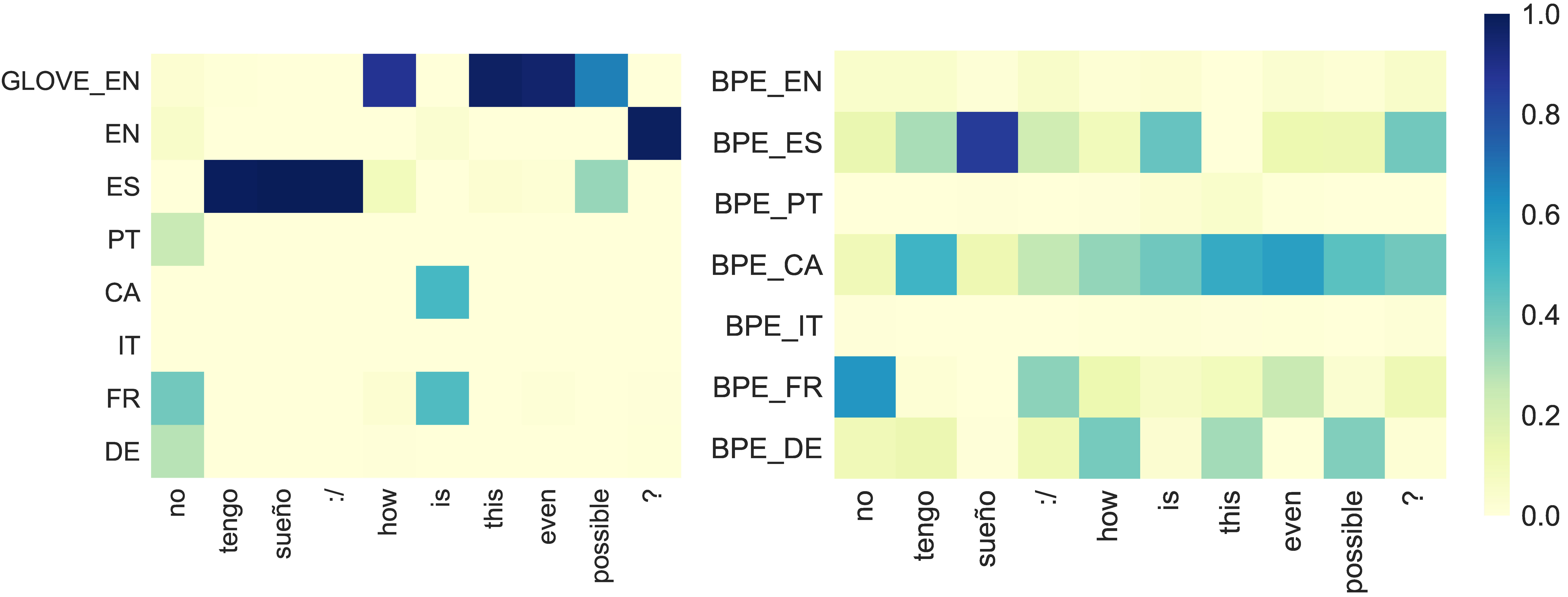
Figure 6.6: Heatmap of attention over languages from a validation sample of the word-level MME and BPE-level MME extracted from the attention weights of the multilingual model (en-es-ca-pt-de-fr-it).

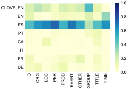
Figure 6.7: The average of attention weights for word embeddings versus NER tags from the validation set.

Visualization

Moreover, we visualize the attention weights of the model at the word and subword-level to interpret the model dynamics. As can be seen from the left-hand side of Figure 6.6, at the word-level, the model mostly chooses the correct language embedding for each word, but also combines different languages. Without any language identifiers, it is impressive to see that our model learns to attend to the right languages. The right-hand side of Figure 6.6, which shows attention weight distributions for the subword-level, demonstrates interesting behaviors of the model, in which, for most English subwords, it leverages ca, fr, and de embeddings. We hypothesize that this is because the dataset is mainly constructed with Spanish words, which can also be verified from Figure 6.7, in which most NER tags are classified as es, and only some as en, such as Group and Time.

6.3 Effectiveness and Efficiency of Multilingual Models

In this section, we provide an analysis on the power of existing pre-trained multilingual models to understand their capability and adaptability in the code-switching setting [145]. Here, we would like to answer the question which models are effective in representing code-switching text, and why?. In order to find the answer, we conduct a comparative study on various existing multilingual models with our proposed meta-embeddings by evaluating the performance, activation memory, and number of parameters. Moreover, we further analyze the memory footprint required by each model over different sequence lengths in a GPU. Thus, we are able to understand which model to choose in a practical scenario.

6.3.1 Experimental Setup

Datasets

We evaluate our models on five downstream tasks and three language pairs in the LinCE Benchmark [2]. We choose three NER tasks, Hindi-English (HIN-ENG) [146], Spanish-English (SPA-ENG) [79] and Modern Standard Arabic (MSA-EA) [79], and two POS tagging tasks, Hindi-English (HIN-ENG) [84] and Spanish-English (SPA-ENG) [147]. For the Hindi-English datasets, we apply Roman-to-Devanagari transliteration. We show the number of tokens of each language in Table 6.7, where we classify the language with more tokens as ML and the other as EL, where ML is the matrix, or the primary, language, and EL is the embedded, or the secondary, language. We replace some words with special tokens, such as user hashtags and mentions with <USR>, emoji with <EMOJI>, and URL with <URL>, for models that use word-embeddings, similarly to Winata et al. [141]. We evaluate our models using the micro-F1 score for NER and accuracy for POS tagging, following Aguilar et al. [2].

Table 6.7: Dataset statistics are taken from Aguilar et al. [2]. We define $L_{1}$ and $L_{2}$ as the languages found in the dataset. For example, in HIN-ENG, $L_{1}$ is HIN and $L_{2}$ is ENG. ^†We define MSA as ML and EA as EL. #$L_{1}$ represents the number of tokens in the first language and #$L_{2}$ represents the number of tokens in the second language.

	#$L_{1}$	#$L_{2}$	ML	EL
NER
HIN-ENG	13,860	11,391	HIN	ENG
SPA-ENG	163,824	402,923	ENG	SPA
MSA-EA†	-	-	MSA	EA
POS
HIN-ENG	12,589	9,882	HIN	ENG
SPA-ENG	178,135	92,517	SPA	ENG

Models

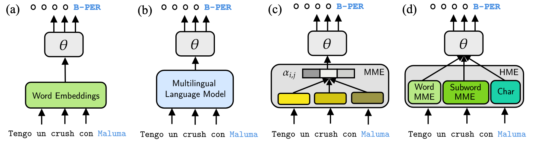
Figure 6.8: Model architectures for code-switched sequence labeling: (a) model using word embeddings, (b) model using multilingual language model, (c) model using multilingual meta-embeddings (MME), and (d) model using hierarchical meta-embeddings (HME).

Here, we compare models: word embedings, bilingual embeddings, and multilingual pre-trained models. We show the general architectures for code-switched sequence labeling in Figure 6.8.

Scratch

We train transformer-based models by following the mBERT model structure, and all of the parameters are randomly initialized. We train transformer models with four and six layers with a hidden size of 768. We want to measure the effectiveness of pre-training on multilingual models. We start the training with a learning rate of 1e-4 and an early stop of 10 epochs.

Word Embeddings

We use FastText embeddings [91, 90] to represent our input in our transformer models. The model consists of a four-layer transformer encoder with four heads and a hidden size of 200. We train a transformer followed by a CRF layer [148]. We train our model with a learning rate of 0.1, a batch size of 32 and an early stop of 10 epochs. We also train our model with only ML and EL embeddings. We freeze all embeddings and only keep the classifier trainable.

Bilingual embeddings

We want to use bilingual embeddings, such as MUSE [104], to align the embeddings space between the ML and EL. We first conduct adversarial training using the SGD optimizer with a learning rate of 0.1, and then we perform the refinement procedure for five iterations using the Procrustes solution and CSLS [104]. After we align the embeddings, we train our model with the aligned word embeddings (MUSE (ML $\rightarrow$ EL) or MUSE (EL $\rightarrow$ ML)) on the code-switching tasks.

Pre-trained Multilingual Models

We use pre-trained models from Huggingface.  On top of each model, we put a fully-connected layer classifier. We train the model with a learning rate between [1e-5, 5e-5] with a decay of 0.1 and a batch size of 8. For large models, such as $\text{XLM-R}_{\text{LARGE}}$ and $\text{XLM-MLM}_{\text{LARGE}}$, we freeze the embeddings layer to fit into a single GPU.

Multilingual Meta-Embeddings (MME)

We use pre-trained word embeddings to train our MME. Table 6.8 shows the embeddings used for each dataset. We freeze all embeddings and train a transformer classifier with the CRF. The transformer classifier consists of a hidden size of 200, a head of 4, and four layers. All models are trained with a learning rate of 0.1, an early stop of 10 epochs, and a batch size of 32. We release the implementation in a public code repository.  Table 6.8 shows the list of word embeddings used in MME.

Hierarchical Meta-Embeddings (HME)

We train our HME model using the same embeddings as MME and pre-trained subword embeddings from Heinzerling and Strube [92]. The word embeddings used in the experiment are shown in Table 6.8 and the subword embeddings for each language pair are shown in Table 6.9. We follow the same hyper-parameters we use when we train MME models.

HME-Ensemble

In order to improve the model’s robustness from multiple predictions, we combine predictions from five HME models, and compute the final prediction by majority voting to achieve a consensus. This method has shown to be very effective in improving the robustness of an unseen test set [149]. The advantage of applying this method is very simple to implement and can be easily spawned in multiple machines, as in parallel processes.

Table 6.8: Embeddings list for MME.

	Word Embeddings List
NER
HIN-ENG	FastText: Hindi, English  [91]
SPA-ENG	FastText: Spanish, English, Catalan,
	Portugese [91]
	GLoVe: English-Twitter [88]
MSA-EA	FastText: Arabic, Egyptian [91]
POS
HIN-ENG	FastText: Hindi, English [91]
SPA-ENG	FastText: Spanish, English, Catalan,
	Portugese [91]
	GLoVe: English-Twitter [88]

Table 6.9: Subword embeddings list for HME.

	Subword Embeddings List
NER
HIN-ENG	Hindi, English
SPA-ENG	Spanish, English, Catalan, Portugese
MSA-EA	Arabic, Egyptian
POS
HIN-ENG	Hindi, English
SPA-ENG	Spanish, English, Catalan, Portugese

Char2Subword

We take the results of the Char2Subword model reported in Aguilar et al. [3].

6.3.2 Results and Discussion

We find that multilingual pre-trained language models, such as $\text{XLM-R}_{\text{BASE}}$, achieves similar or sometimes better results than the HME model. Note that HME uses word and subword pre-trained embeddings that are trained using significantly fewer data than mBERT and $\text{XLM-R}_{\text{BASE}}$ and can achieve on par performance to theirs. Interestingly, we also observed that $\text{XLM-R}_{\text{LARGE}}$ improves the performance significantly, but with a trade-off in the training and inference time, with 13x more parameters than HME-Ensemble for a marginal improvement (2%). We evaluate all the models on the LinCE benchmark, and the development set results are shown in Table 6.10. As expected, the Scratch models perform significantly worse than the other pre-trained models. Both FastText and MME use pre-trained word embeddings, but MME achieves a consistently higher F1 score than FastText in both NER and POS tasks. This demonstrates the importance of the contextualized self-attentive encoder. HME further improves on the F1 score of the MME models, suggesting that encoding hierarchical information from subword-level, word-level, and sentence-level representations can improve the code-switching task performance. Comparing HME with mBERT and XLM-R, we find that the HME models are able to obtain comparable F1 scores with up to 10x smaller model sizes, and this indicates that pre-trained multilingual word embeddings can achieve a good balance between performance and model size in code-switching tasks. We show the model’s performance on the LinCE benchmark test set in Table 6.11. $\text{XLM-R}_{\text{LARGE}}$ achieves the best-average performance, with a 13x larger model size when we compare it to the HME-Ensemble model.

Table 6.10: Results on the development set of the LinCE benchmark. ^‡ The results are taken from Aguilar et al. [3]. The number of parameters of mBERT (cased) is calculated by approximation.

		NER						POS
		HIN-ENG		SPA-ENG		MSA-EA		HIN-ENG		SPA-ENG
Method	Avg Perf.	Params	F1	Params	F1	Params	F1	Params	Acc	Params	Acc
Scratch (2L)	63.40	96M	46.51	96M	32.75	96M	60.14	96M	83.20	96M	94.39
Scratch (4L)	60.93	111M	47.01	111M	19.06	111M	60.24	111M	83.72	111M	94.64
Mono/Multilingual Word Embeddings
FastText (ML)	76.43	4M	63.58	18M	57.10	16M	78.42	4M	84.63	6M	98.41
FastText (EL)	76.71	4M	69.79	18M	58.34	16M	72.68	4M	84.40	6M	98.36
MUSE (ML $\rightarrow$ EL)	76.54	4M	64.05	18M	58.00	16M	78.50	4M	83.82	6M	98.34
MUSE (EL $\rightarrow$ ML)	75.58	4M	64.86	18M	57.08	16M	73.95	4M	83.62	6M	98.38
Pre-Trained Multilingual Models
mBERT (uncased)	79.46	167M	68.08	167M	63.73	167M	78.61	167M	90.42	167M	96.48
mBERT (cased)‡	79.97	177M	72.94	177M	62.66	177M	78.93	177M	87.86	177M	97.29
Char2Subword‡	81.07	136M	74.91	136M	63.32	136M	80.45	136M	89.64	136M	97.03
$\text{XLM-R}_{\text{BASE}}$	81.90	278M	76.85	278M	62.76	278M	81.24	278M	91.51	278M	97.12
XLM-R${}_{\text{LARGE}}$	84.39	565M	79.62	565M	67.18	565M	85.19	565M	92.78	565M	97.20
$\text{XLM-MLM}_{\text{LARGE}}$	81.41	572M	73.91	572M	62.89	572M	82.72	572M	90.33	572M	97.19
Multilingual Meta-Embeddings
Concat	79.70	10M	70.76	86M	61.65	31M	79.33	8M	88.14	23M	98.61
Linear	79.60	10M	69.68	86M	61.74	31M	79.42	8M	88.58	23M	98.58
Attention (MME)	79.86	10M	71.69	86M	61.23	31M	79.41	8M	88.34	23M	98.65
HME	81.60	12M	73.98	92M	62.09	35M	81.26	12M	92.01	30M	98.66
HME-Ensemble	82.44	20M	76.16	103M	62.80	43M	81.67	20M	92.84	40M	98.74

Table 6.11: Results on the test set of the LinCE benchmark.^‡ The results are taken from Aguilar et al. [3]. ^† The result is taken from the LinCE leaderboard.

			NER			POS
Method	Avg Params	Avg Perf.$\uparrow$	HIN-ENG	SPA-ENG	MSA-EA	HIN-ENG	SPA-ENG
English BERT (cased)†	108M	75.80	74.46	61.15	59.44	87.02	96.92
mBERT (cased)‡	177M	77.08	72.57	64.05	65.39	86.30	97.07
HME	36M	77.64	73.78	63.06	66.14	88.55	96.66
Char2Subword‡	136M	77.85	73.38	64.65	66.13	88.23	96.88
XLM-MLM${}_{\text{LARGE}}$	572M	78.40	74.49	64.16	67.22	89.10	97.04
XLM-R${}_{\text{BASE}}$	278M	78.75	75.72	64.95	65.13	91.00	96.96
HME-Ensemble	45M	79.17	75.97	65.11	68.71	89.30	96.78
XLM-R${}_{\text{LARGE}}$	565M	80.96	80.70	69.55	65.78	91.59	97.18

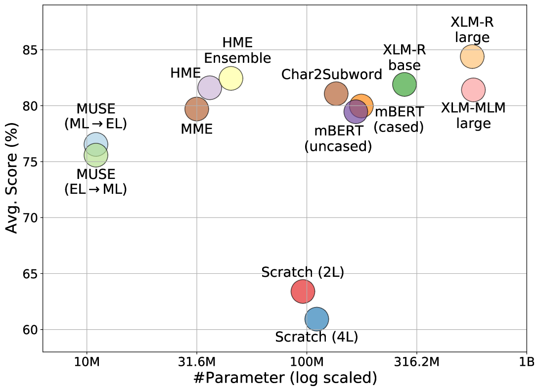
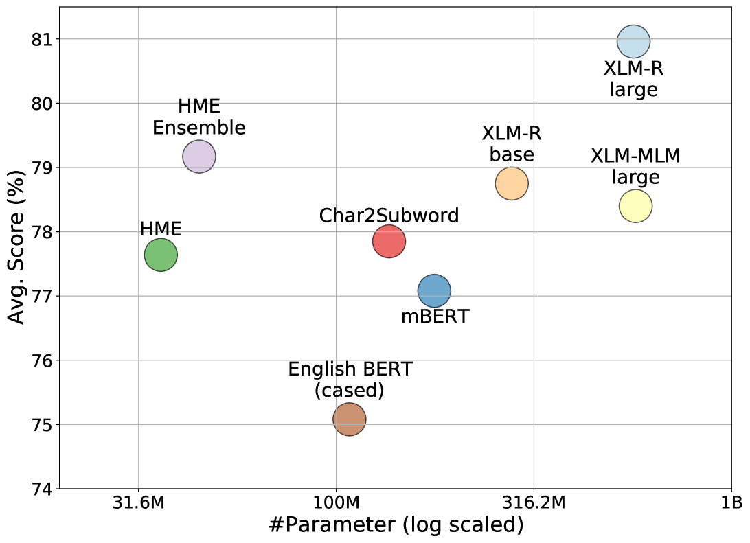
Figure 6.9: Validation set (left) and test set (right) evaluation performance (y-axis) and parameter (x-axis) of different models on LinCE benchmark.

Performance vs. Model Size

As shown in Figure 6.9, the Scratch models yield the worst average score, at 60.93 points. The model performance can be improved by around 10 points by using pre-trained embeddings FastText with only 10M parameters on average. On the other hand, the MME models, which have 31.6M parameters on average, achieve similar results to the mBERT models, with around 170M parameters. Interestingly, adding subwords and character embeddings to MME, such as in the HME models, further improves the performance of the MME models and achieves a 81.60 average score, similar to that of the XLM-R${}_{\text{BASE}}$ and XLM-MLM${}_{\text{LARGE}}$ models, but with less than one-fifth the number of parameters, at around 42.25M. The ensemble method adds further performance improvement of the HME model by around 1%, with an additional 2.5M parameters compared to its non-ensemble counterparts.

Inference Time

To compare the speed of different models, we generate data with random values and various sequence lengths: [16, 32, 64, 128, 256, 512, 1024, 2048, 4096]. We measure each model’s inference time and collect the statistics of each at a particular sequence length by running the model 100 times. The experiment is performed on a single NVIDIA GTX1080Ti GPU. We do not include the pre-processing time in our analysis. It is evident that the pre-processing time for the meta-embeddings models is longer than for other models as pre-processing requires a tokenization step to be conducted for the input multiple times with different tokenizers. The reported sequence lengths are counted based on the input tokens of each model, and we use words for the MME and HME models, and subwords for the other models.

We show the results of the inference speed test in Figure 6.10. Although all pre-trained contextualized language models yield a high validation score, these models are the slowest in terms of inference time. The larger the size of the pre-trained model, the longer it takes to run a prediction. For shorter sequences, the HME model performs as quickly as the mBERT and XLM-R${}_{\text{BASE}}$ models, and can retain its speed as the sequence length increases because of the smaller model dimensions in each layer. The FastText, MME, and Scratch models have high throughput in short-sequence settings by processing more than 150 samples per second. For longer sequences, the same behavior occurs, with the throughput of the Scratch models reducing as the sequence length increases, even becoming lower than that of the HME model when the sequence length is greater than or equal to 256. In addition, for the FastText, MME, and HME models, the throughput remains steady when the sequence length is less than 1024, and it starts to decrease afterwards.

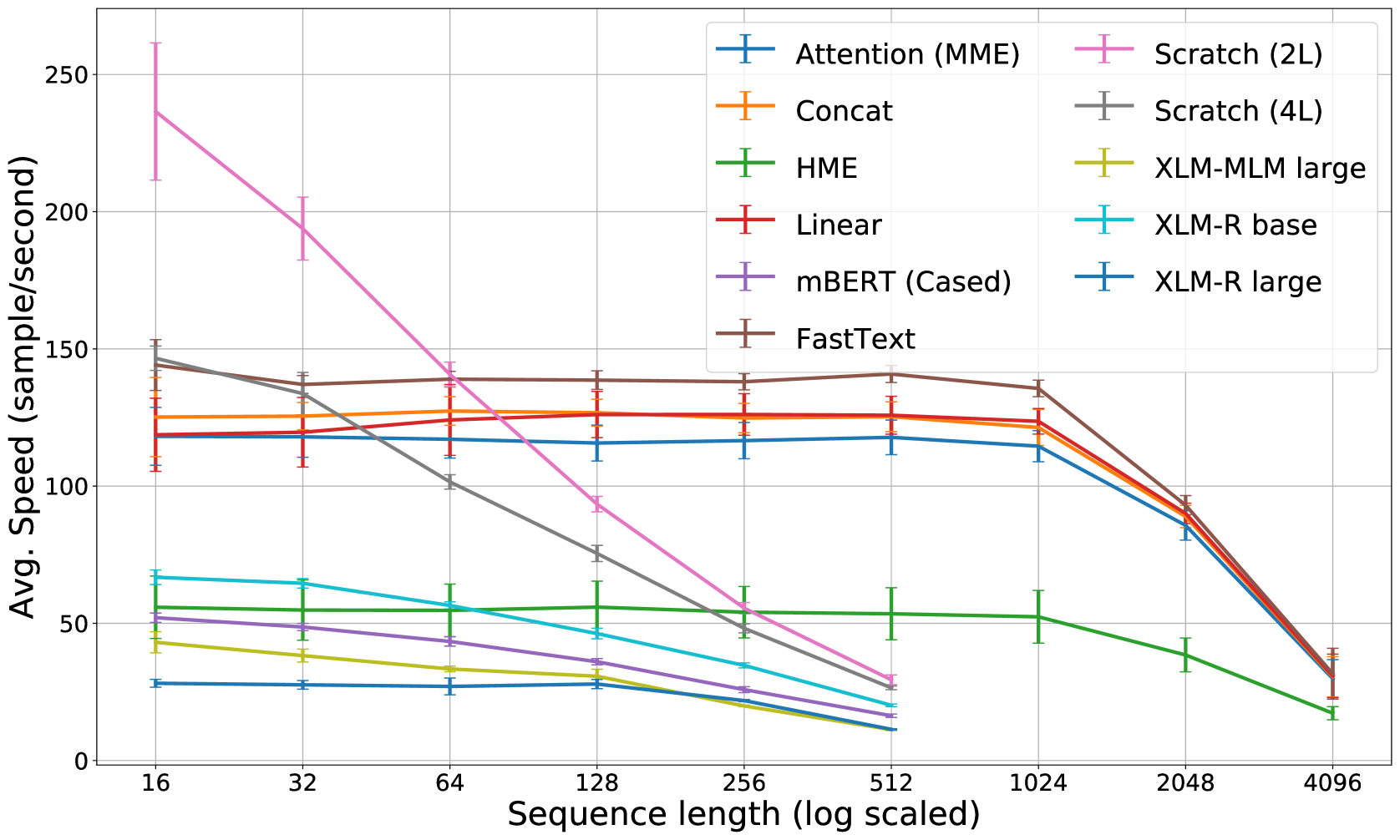
Figure 6.10: Speed-to-sequence length comparison of different models.

Table 6.12: GPU memory consumption of different models with input size of 512.

Model	Activation (MB)
FastText	79.0
Concat	85.3
Linear	80.8
Attention (MME)	88.0
HME	154.8
Scratch (2L)	133.0
Scratch (4L)	264.0
mBERT	597.0
XLM-R${}_{\text{BASE}}$	597.0
XLM-R${}_{\text{LARGE}}$	1541.0
XLM-MLM${}_{\text{LARGE}}$	1158.0

Memory Footprint

We record the memory footprint over different sequence lengths, and use the same setting for the FastText, MME, and HME models as in the inference time analysis. We record the size of each model on a GPU machine, and the size of the activation memory after performing a single forward operation on a sample with a certain sequence length. The result of the memory footprint analysis for a sequence length of 512 is shown in Table 6.12. Based on the results, we can see that the meta-embedding models use a significantly smaller memory footprint to store the model and activation memory. For example, the memory footprint of the HME model is less than that of the Scratch (4L) model, which has only four transformer encoder layers, a model dimension of 768 and a feed-forward dimension of 3,072. On the other hand, large pre-trained language models, such as XLM-MLM${}_{\text{LARGE}}$ and XLM-R${}_{\text{LARGE}}$, use a much larger memory for storing the activation memory compared to all other models. The complete results of the memory footprint analysis can be found in Appendix.

6.4 Short Summary

In this chapter, we propose two approaches for learning representations for code-switching data. First, we introduce a BiLSTM-based model with a hierarchical architecture using a bilingual character RNN to address the OOV words issue. Moreover, token replacement, token normalization, and transfer learning reduce the OOV words rate even further and significantly improves the performance. We show that our model can achieve similar performance to models using gazetteers and hand-picked features. Then, we propose Hierarchical Meta-Embeddings (HME), which learns how to combine multiple monolingual word-level and subword-level embeddings to create language-agnostic representations without specific language information. We achieve the state-of-the-art results on the task of NER for English-Spanish code-switching data. We also show that our model can leverage subword information very effectively from languages from different roots to generate better word representations.

We study the effectiveness of multilingual language models so as to understand their capability and adaptability to the code-switching setting. We run experiments on NER and POS tagging on three different language pairs, and find that a pre-trained multilingual model does not necessarily guarantee high-quality representations on code-switching, while the HME model achieves similar results to mBERT and $\text{XLM-R}_{\text{BASE}}$, but with significantly fewer parameters. We also find that, while $\text{XLM-R}_{\text{LARGE}}$ has better performance by a large margin, this comes with a substantial cost in the training and inference time, using 13x more parameters than HME-Ensemble for only a 2% improvement.

Chapter 7 Conclusion

This thesis focuses on transfer learning methods for code-switching NLP and speech processing tasks by leveraging monolingual resources. We discussed the main challenges in code-switching and introduced novel transfer learning approaches for language modeling, speech recognition, and representation learning for sequence labeling tasks. We proposed multilingual transfer learning by utilizing monolingual data to improve code-switching representations to address the need for huge amounts of data. In this chapter, we conclude the thesis, summarize our contributions, and discuss possible future work.

We examined data augmentation approaches to train language models for code-switching by generating synthetic code-switching data using a neural network language model with a copy mechanism, called Pointer-Gen. Pointer-Gen leverages information from the input to ensure high-quality code-switching sentence generation and eliminates the dependence on the aligner or tagger. It learns the distribution of the real code-switching data instead of relying on the linguistic prior information. The proposed approach increases the variance of the corpus to increase the robustness of our language models. Pointer-Gen samples new code-switching sentences from the distribution of the code-switching data in a zero-shot setting. The model works effectively for the English-Mandarin language pair, in which the languages are inherently different in terms of their grammatical structure. We found that our data augmentation method outperforms the method with an equivalence constraint and other neural-based augmentation methods.

We presented approaches to train language models with multi-task training that leverages syntactic information. We train our model by jointly learning the language modeling task and part-of-speech sequence tagging task on code-switched utterances. We incorporate language information into part-of-speech tags to create bilingual tags that distinguish between languages, and learn the correlation between language modeling and the next part-of-speech prediction. Indeed, the syntactic information helps the model to be aware of code-switching points, and it boosts the performance over the language model.

We introduced multi-task learning approaches to train code-switching speech recognition by proposing transfer learning methods. Our methods apply meta-learning by judiciously extracting information from high-resource monolingual datasets. The optimization conditions the model to retrieve useful learned information that is focused on the code-switching domain. The meta-transfer learning quickly adapts the model to the code-switching task from a number of monolingual tasks by learning to learn. Experimental results showed that our proposed method preserves the monolingual tasks’ performance, and it is faster to converge.

We discussed state-of-the-art multilingual representation learning methods for code-switched named entity recognition. We introduced meta-embeddings considering the commonalities across languages and lexical compositionality. We found that this method is language-agnostic, and it is very effective and efficient compared to large contextual language models, such as mBERT and XLM-R in the code-switching domain. We also found that the hierarchical meta-embeddings model obtains comparable F1 and accuracy scores with up to 10x smaller model sizes compared to pre-trained multilingual models.

Lastly, the main contribution of this thesis is that it emphasizes the importance of multilingual transfer learning on code-switching tasks. We proposed language-agnostic end-to-end approaches that are not dependent on particular languages to improve the generalization of our models on code-switched data. And, the transfer learning from monolingual data is very effective for code-switching. It is also worth noting that linguistic theory can be used as prior information to understand how code-switches are triggered.

In future work, we expect to develop a better training objective to learn a multilingual contextualized language model in a self-supervised fashion that can well represent mixed languages since, according to our empirical observation, the current pre-trained models lack cross-linguality. We would also like to explore a more effective transfer learning method to leverage monolingual data and parallel data.

List of Publications

(* denotes equal contribution)

• Zihan Liu, Genta Indra Winata, Samuel Cahyawijaya, Andrea Madotto, Zhaojiang Lin, Pascale Fung. ”On the Importance of Word Order Information in Cross-lingual Sequence Labeling.” In AAAI, 2021.

• Andrea Madotto, Samuel Cahyawijaya, Genta Indra Winata, Yan Xu, Zihan Liu, Zhaojiang Lin, Pascale Fung. ”Learning Knowledge Bases with Parameters for Task-Oriented Dialogue Systems.” In Proceedings of the 2020 Conference on Empirical Methods in Natural Language Processing: Findings, 2020.

• Zihan Liu, Genta Indra Winata, Peng Xu, Zhaojiang Lin, Pascale Fung. ”Cross-lingual Spoken Language Understanding with Regularized Representation Alignment.” In Proceedings of the 2020 Conference on Empirical Methods in Natural Language Processing (EMNLP), 2020.

• Zhaojiang Lin, Andrea Madotto, Genta Indra Winata, Pascale Fung. ”MinTL: Minimalist transfer learning for task-oriented dialogue systems.” Proceedings of the 2020 Conference on Empirical Methods in Natural Language Processing (EMNLP), 2020.

• Bryan Wilie*, Karissa Vincentio*, Genta Indra Winata*, Samuel Cahyawijaya*, Xiaohong Li, Zhi Yuan Lim, Sidik Soleman, Rahmad Mahendra, Pascale Fung, Syafri Bahar, Ayu Purwarianti. ”IndoNLU: Benchmark and resources for evaluating indonesian natural language understanding.” In Proceedings of the 1st Conference of the Asia-Pacific Chapter of the Association for Computational Linguistics and the 10th International Joint Conference on Natural Language Processing, 2020.

• Genta Indra Winata*, Samuel Cahyawijaya*, Zhaojiang Lin, Zihan Liu, Peng Xu, Pascale Fung. ”Meta-transfer learning for code-switched speech recognition.” In Proceedings of the 58th Annual Meeting of the Association for Computational Linguistics, 2020.

• Zihan Liu, Genta Indra Winata, Peng Xu, Pascale Fung. ”Coach: A Coarse-to-Fine Approach for Cross-domain Slot Filling.” In Proceedings of the 58th Annual Meeting of the Association for Computational Linguistics, 2020.

• Genta Indra Winata*, Samuel Cahyawijaya*, Zihan Liu*, Zhaojiang Lin, Andrea Madotto, Peng Xu, Pascale Fung. ”Learning Fast Adaptation on Cross-Accented Speech Recognition.” In INTERSPEECH, 2020.

• Zihan Liu*, Genta Indra Winata*, Zhaojiang Lin, Peng Xu, Pascale Fung. ”Attention-Informed Mixed-Language Training for Zero-shot Cross-lingual Task-oriented Dialogue Systems.” In AAAI, 2020.

• Genta Indra Winata*, Samuel Cahyawijaya*, Zhaojiang Lin, Zihan Liu, and Pascale Fung. ”Lightweight and Efficient End-to-End Speech Recognition Using Low-Rank Transformer.” In ICASSP 2020-2020 IEEE International Conference on Acoustics, Speech and Signal Processing (ICASSP), pp. 6144-6148. IEEE, 2020.

• Zhaojiang Lin, Peng Xu, Genta Indra Winata, Farhad Bin Siddique, Zihan Liu, Jamin Shin, and Pascale Fung. ”CAiRE: An End-to-End Empathetic Chatbot.” In AAAI, pp. 13622-13623. 2020.

• Zihan Liu, Jamin Shin, Yan Xu, Genta Indra Winata, Peng Xu, Andrea Madotto, and Pascale Fung. ”Zero-shot Cross-lingual Dialogue Systems with Transferable Latent Variables.” In Proceedings of the 2019 Conference on Empirical Methods in Natural Language Processing and the 9th International Joint Conference on Natural Language Processing (EMNLP-IJCNLP), pp. 1297-1303. 2019.

• Genta Indra Winata, Zhaojiang Lin, Jamin Shin, Zihan Liu, and Pascale Fung. ”Hierarchical Meta-Embeddings for Code-Switching Named Entity Recognition.” In Proceedings of the 2019 Conference on Empirical Methods in Natural Language Processing and the 9th International Joint Conference on Natural Language Processing (EMNLP-IJCNLP), pp. 3532-3538. 2019.

• Genta Indra Winata, Andrea Madotto, Chien-Sheng Wu, and Pascale Fung. ”Code-Switched Language Models Using Neural Based Synthetic Data from Parallel Sentences.” In Proceedings of the 23rd Conference on Computational Natural Language Learning (CoNLL), pp. 271-280. 2019.

• Genta Indra Winata, Andrea Madotto, Jamin Shin, Elham J. Barezi, and Pascale Fung. ”On the Effectiveness of Low-Rank Matrix Factorization for LSTM Model Compression.” Proceedings of the 33rd Pacific Asia Conference on Language, Information and Computation (PACLIC), 2019.

• Zhaojiang Lin, Genta Indra Winata, and Pascale Fung. ”Learning comment generation by leveraging user-generated data.” In ICASSP 2019-2019 IEEE International Conference on Acoustics, Speech and Signal Processing (ICASSP), pp. 7225-7229. IEEE, 2019.

• Dan Su, Yan Xu, Genta Indra Winata, Peng Xu, Hyeondey Kim, Zihan Liu, and Pascale Fung. ”Generalizing Question Answering System with Pre-trained Language Model Fine-tuning.” In EMNLP 2019 MRQA Workshop, p. 203. 2019.

• Zihan Liu, Yan Xu, Genta Indra Winata, and Pascale Fung. ”Incorporating Word and Subword Units in Unsupervised Machine Translation Using Language Model Rescoring.” In Proceedings of the Fourth Conference on Machine Translation (Volume 2: Shared Task Papers, Day 1), pp. 275-282. 2019.

• Genta Indra Winata*, Andrea Madotto*, Zhaojiang Lin, Jamin Shin, Yan Xu, Peng Xu, and Pascale Fung. ”CAiRE_HKUST at SemEval-2019 Task 3: Hierarchical Attention for Dialogue Emotion Classification.” In Proceedings of the 13th International Workshop on Semantic Evaluation, pp. 142-147. 2019.

• Genta Indra Winata, Zhaojiang Lin, and Pascale Fung. ”Learning multilingual meta-embeddings for code-switching named entity recognition.” In Proceedings of the 4th Workshop on Representation Learning for NLP (RepL4NLP-2019), pp. 181-186. 2019.

• Zhaojiang Lin, Andrea Madotto, Genta Indra Winata, Zihan Liu, Yan Xu, Cong Gao, and Pascale Fung. ”Learning to learn sales prediction with social media sentiment.” In Proceedings of the First Workshop on Financial Technology and Natural Language Processing, pp. 47-53. 2019.

• Genta Indra Winata, Chien-Sheng Wu, Andrea Madotto, and Pascale Fung. ”Bilingual Character Representation for Efficiently Addressing Out-of-Vocabulary Words in Code-Switching Named Entity Recognition.” In Proceedings of the Third Workshop on Computational Approaches to Linguistic Code-Switching, pp. 110-114. 2018.

• Genta Indra Winata, Andrea Madotto, Chien-Sheng Wu, and Pascale Fung. ”Code-Switching Language Modeling using Syntax-Aware Multi-Task Learning.” In Proceedings of the Third Workshop on Computational Approaches to Linguistic Code-Switching, pp. 62-67. 2018.

• Chien-Sheng Wu, Andrea Madotto, Genta Indra Winata, and Pascale Fung. ”End-to-end dynamic query memory network for entity-value independent task-oriented dialog.” In 2018 IEEE International Conference on Acoustics, Speech and Signal Processing (ICASSP), pp. 6154-6158. IEEE, 2018.

• Genta Indra Winata, Onno Pepijn Kampman, and Pascale Fung. ”Attention-based lstm for psychological stress detection from spoken language using distant supervision.” In 2018 IEEE International Conference on Acoustics, Speech and Signal Processing (ICASSP), pp. 6204-6208. IEEE, 2018.

• Genta Indra Winata, Onno Kampman, Yang Yang, Anik Dey, and Pascale Fung. ”Nora the Empathetic Psychologist.” In INTERSPEECH, pp. 3437-3438. 2017.

• Chien-Sheng Wu*, Andrea Madotto*, Genta Winata, and Pascale Fung. ”End-to-end recurrent entity network for entity-value independent goal-oriented dialog learning.” In Dialog System Technology Challenges Workshop, DSTC6. 2017.

Appendix

Multi-Task Learning Results

Results with different hyper-parameter settings

Table 1: Language model results in Phase I

Model	Hidden size	Embedding size	Dropout	POS tag dropout	PPL dev	PPL test
LSTM	200	200	0.2	-	197.5	196.84
	500	500	0.4	-	190.33	185.91
+ syntactic features	200	200	0.2	-	187.37	184.87
	500	500	0.4	-	178.51	176.57
Multi-task ($p=0.25$)	200	200	0.4	0.2	180.91	178.18
	500	500	0.4	0.4	173.55	174.96
Multi-task ($p=0.50$)	200	200	0.4	0.2	182.6	178.75
	500	500	0.4	0.4	175.23	173.89
Multi-task ($p=0.75$)	200	200	0.4	0.2	180.90	178.18
	500	500	0.4	0.4	185.83	178.49

Table 2: Language model results in SEAME Phase II

Model	Hidden size	Embedding size	Dropout	POS tag dropout	PPL dev	PPL test
RNNLM	200	200	-	-	181.87	176.80
	500	500	-	-	178.35	171.27
LSTM	200	200	0.2	-	156.77	159.58
	500	500	0.4	-	150.65	153.06
+ syntactic features	200	200	0.2	-	153.6	152.66
	500	500	0.4	-	147.44	148.38
Multi-task ($p=0.25$)	200	200	0.4	0.2	149.68	149.84
	500	500	0.4	0.4	141.86	141.71
Multi-task ($p=0.50$)	200	200	0.4	0.2	150.92	152.38
	500	500	0.4	0.4	144.18	144.27
Multi-task ($p=0.75$)	200	200	0.4	0.2	150.32	151.22
	500	500	0.4	0.4	145.08	144.85

SEAME Data Split

We split the recording ids into train, development, and test set as the following:

Table 3: Recording distribution in Phase I

Data	Recording list
	Conversation	Interview
Train	02NC03FBX, 02NC04FBY, 03NC05FAX 03NC06FAY,04NC07FBX,04NC08FBY 06NC11MAX,06NC12MAY,07NC13MBP 07NC14FBQ,08NC15MBP,08NC16FBQ 09NC17FBP,09NC18MBQ,10NC19MBP 10NC20MBQ,11NC21FBP,11NC22MBQ 12NC23FBP,12NC24FBQ,13NC25MBP 13NC26MBQ,14NC27MBP,14NC28MBQ 16NC31FBP,16NC32FBQ,18NC35FBP 18NC36MBQ,19NC37MBP,19NC38FBQ 21NC41MBP,22NC43FBP,22NC44MBQ 23NC35FBQ,23NC45MBP,24NC35FBQ 24NC45MBP,25NC43FBQ,25NC47MBP 26NC48FBP,26NC49FBQ,27NC47MBQ 27NC50FBP,28NC51MBP,28NC52FBQ 29NC53MBP,29NC54FBQ,30NC48FBP 30NC49FBQ,31NC35FBQ,31NC50XFB 32NC36MBQ,32NC50FBP,33NC37MBP 33NC43FBQ,34NC37MBP,35NC56MBP 36NC46FBQ,37NC45MBP,38NC50FBP 39NC57FBX,40NC58FAY,41NC59MAX 42NC60FBQ,44NC44MBQ,45NC22MBQ 46NC41MBP,46NC41MBP	NI02FAX,NI04FBX,NI05MBQ NI06FBP,NI07FBQ,NI08FBP NI09FBP,NI10FBP,NI11FBP NI12MAP,NI13MBQ,NI14MBP NI15FBQ,NI16FBP,NI17FBQ NI18MBP,NI19MBQ,NI20MBP NI21MBQ,NI22FBP,NI23FBQ NI24MBP,NI25MBQ,NI26FBP NI27MBQ,NI28MBP,NI29MBP NI30MBQ,NI31FBP,NI32FBQ NI33MBP,NI34FBQ,NI35FBP NI36MBQ,NI37MBP,NI39FBP NI40FBQ,NI41MBP,NI42FBQ NI43FBP,NI44MBQ,NI45FBP NI46FBQ,NI47MBP,NI48FBQ NI49MBP,NI50FBQ,NI51MBP NI52MBQ,NI53FBP,NI54FBQ NI55FBP,NI56MBX,NI57FBQ NI58FBP,NI59FBQ,NI60MBP NI61FBP,NI62MBQ,NI63MBP NI64FBQ,NI65MBP,NI66MBQ NI67MBQ,UI02FAZ,UI03FAZ UI04FAZ,UI05MAZ,UI06MAZ UI07FAZ,UI08MAZ,UI10FAZ UI11FAZ,UI12FAZ,UI13FAZ UI14MAZ,UI15FAZ,UI16MAZ UI17FAZ,UI18MAZ,UI19MAZ UI20MAZ,UI21MAZ,UI22MAZ UI23FAZ,UI24MAZ,UI25FAZ UI26MAZ,UI27FAZ,UI28FAZ UI29FAZ
Dev	01NC01FBX, 01NC02FBY, 15NC29FBP 15NC30MBQ, 21NC42MBQ, 43NC61FBQ	UI01FAZ, UI09MAZ
Test	05NC09FAX, 05NC10MAY, 17NC33FBP 17NC34FBQ, 20NC39MBP, 20NC40FBQ	NI01MAX, NI03FBX

Table 4: Recording distribution in Phase II

Data	Recording list
	Conversation	Interview
Train	02NC03FBX, 02NC04FBY, 03NC05FAX 03NC06FAY, 04NC07FBX, 04NC08FBY 06NC11MAX, 06NC12MAY, 07NC13MBP 07NC14FBQ, 08NC15MBP, 08NC16FBQ 09NC17FBP, 09NC18MBQ, 10NC19MBP 10NC20MBQ, 11NC21FBP, 11NC22MBQ 12NC23FBP, 12NC24FBQ, 13NC25MBP 13NC26MBQ, 14NC27MBP, 14NC28MBQ 16NC31FBP, 16NC32FBQ, 18NC35FBP 18NC36MBQ, 19NC37MBP, 19NC38FBQ 21NC41MBP, 22NC43FBP, 22NC44MBQ 23NC35FBQ, 23NC45MBP, 24NC35FBQ 24NC45MBP, 25NC43FBQ, 25NC47MBP 26NC48FBP, 26NC49FBQ, 27NC47MBQ 27NC50FBP, 28NC51MBP, 28NC52FBQ 29NC53MBP, 29NC54FBQ, 30NC48FBP 30NC49FBQ, 31NC35FBQ, 31NC50XFB 32NC36MBQ, 32NC50FBP, 33NC37MBP 33NC43FBQ, 34NC37MBP, 35NC56MBP 36NC46FBQ, 37NC45MBP, 38NC50FBP 39NC57FBX, 40NC58FAY, 41NC59MAX 42NC60FBQ, 44NC44MBQ, 45NC22MBQ 46NC41MBP	NI02FAX, NI04FBX, NI05MBQ NI06FBP, NI07FBQ, NI08FBP NI09FBP, NI10FBP, NI12MAP NI13MBQ, NI14MBP, NI15FBQ NI16FBP, NI17FBQ, NI18MBP NI19MBQ, NI20MBP, NI21MBQ NI22FBP, NI23FBQ, NI24MBP NI25MBQ, NI26FBP, NI27MBQ NI28MBP, NI29MBP, NI30MBQ NI31FBP, NI32FBQ, NI33MBP NI34FBQ, NI35FBP, NI36MBQ NI37MBP, NI39FBP, NI40FBQ NI41MBP, NI42FBQ, NI43FBP NI44MBQ, NI45FBP, NI46FBQ NI47MBP, NI48FBQ, NI49MBP NI50FBQ, NI51MBP, NI52MBQ NI53FBP, NI54FBQ, NI55FBP NI56MBX, NI57FBQ, NI58FBP NI59FBQ, NI60MBP, NI61FBP NI62MBQ, NI63MBP, NI64FBQ NI65MBP, NI66MBQ, NI67MBQ UI02FAZ, UI03FAZ, UI04FAZ UI05MAZ, UI06MAZ, UI07FAZ UI08MAZ, UI10FAZ, UI11FAZ UI12FAZ, UI13FAZ, UI14MAZ UI15FAZ, UI16MAZ, UI17FAZ UI18MAZ, UI19MAZ, UI20MAZ UI21MAZ, UI22MAZ, UI23FAZ UI24MAZ, UI25FAZ, UI26MAZ UI27FAZ, UI28FAZ, UI29FAZ
Dev	01NC01FBX, 01NC02FBY, 15NC29FBP 15NC30MBQ, 21NC42MBQ, 43NC61FBQ	UI01FAZ, UI09MAZ
Test	05NC09FAX, 05NC10MAY, 17NC33FBP 17NC34FBQ, 20NC39MBP, 20NC40FBQ	NI01MAX, NI03FBX

Memory Footprint Analysis

We show the complete results of our memory footprint analysis of word-embeddings, meta-embeddings, and multilingual models in Table 5.

Table 5: Memory footprint (MB) for storing the activations for a given sequence length.

Model	Activation (MB)
	16	32	64	128	256	512	1024	2048	4096
FastText	1.0	2.0	4.0	10.0	26.0	79.0	261.0	941.0	3547.0
Linear	1.0	2.0	4.0	10.0	27.4	80.8	265.6	950.0	3562.0
Concat	1.0	2.0	5.0	11.2	29.2	85.2	274.5	967.5	3596.5
Attention (MME)	1.0	2.0	5.4	12.4	31.0	89.0	283.2	985.6	3630.6
HME	3.2	6.6	13.4	28.6	64.2	154.8	416.4	1252.0	4155.0
Scratch (2L)	2.0	4.0	8.0	20.0	46.0	133.0	-	-	-
Scratch (4L)	3.0	7.0	15.0	38.0	90.0	264.0	-	-	-
mBERT (uncased)	10.0	20.0	41.0	100.0	218.0	597.0	-	-	-
XLM-R${}_{\text{BASE}}$	10.0	20.0	41.0	100.0	218.0	597.0	-	-	-
XLM-R${}_{\text{LARGE}}$	25.0	52.0	109.0	241.0	579.0	1541.0	-	-	-
XLM-MLM${}_{\text{LARGE}}$	20.0	42.0	89.0	193.0	467.0	1158.0	-	-	-

References

- Pratapa et al. [2018a] A. Pratapa, G. Bhat, M. Choudhury, S. Sitaram, S. Dandapat, and K. Bali, “Language modeling for code-mixing: The role of linguistic theory based synthetic data,” in Proceedings of the 56th Annual Meeting of the Association for Computational Linguistics (Volume 1: Long Papers), vol. 1, 2018, pp. 1543–1553.
- Aguilar et al. [2020a] G. Aguilar, S. Kar, and T. Solorio, “Lince: A centralized benchmark for linguistic code-switching evaluation,” in Proceedings of The 12th Language Resources and Evaluation Conference, 2020, pp. 1803–1813.
- Aguilar et al. [2020b] G. Aguilar, B. McCann, T. Niu, N. Rajani, N. Keskar, and T. Solorio, “Char2subword: Extending the subword embedding space from pre-trained models using robust character compositionality,” arXiv preprint arXiv:2010.12730, 2020.
- Tucker [1999] G. R. Tucker, “A global perspective on bilingualism and bilingual education,” Georgetown University Round Table on Languages and Linguistics, pp. 332–340, 1999.
- Poplack [1980] S. Poplack, “Sometimes i’ll start a sentence in spanish y termino en espanol: Toward a typology of code-switching1,” Linguistics, vol. 18, no. 7-8, pp. 581–618, 1980.
- Bullock and Toribio [2009] B. Bullock and A. Toribio, The Cambridge Handbook of Linguistic Code-switching (Cambridge Handbooks in Language and Linguistics). Cambridge University Press, 2009.
- Anderson and Toribio [2007] T. K. Anderson and A. J. Toribio, “Attitudes towards lexical borrowing and intra-sentential code-switching among spanish-english bilinguals,” Spanish in Context, vol. 4, no. 2, pp. 217–240, 2007.
- Rothman and Rell [2007] J. Rothman and A. B. Rell, “A linguistic analysis of spanglish: Relating language to identity,” Linguistics and the Human Sciences, vol. 1, no. 3, pp. 515–536, 2007.
- Rizal and Stymne [2020] A. N. Rizal and S. Stymne, “Evaluating word embeddings for Indonesian–English code-mixed text based on synthetic data,” in Proceedings of the The 4th Workshop on Computational Approaches to Code Switching. Marseille, France: European Language Resources Association, May 2020, pp. 26–35. [Online]. Available: https://www.aclweb.org/anthology/2020.calcs-1.4
- Ng et al. [2005] T. P. Ng, L. C. C. Lim, A. Jin, and N. Shinfuku, “Ethnic differences in quality of life in adolescents among chinese, malay and indians in singapore,” Quality of Life Research, vol. 14, no. 7, pp. 1755–1768, 2005.
- Vyas et al. [2014] Y. Vyas, S. Gella, J. Sharma, K. Bali, and M. Choudhury, “Pos tagging of english-hindi code-mixed social media content,” in Proceedings of the 2014 Conference on Empirical Methods in Natural Language Processing (EMNLP), 2014, pp. 974–979.
- Barman et al. [2016] U. Barman, J. Wagner, and J. Foster, “Part-of-speech tagging of code-mixed social media content: Pipeline, stacking and joint modelling,” in Proceedings of the Second Workshop on Computational Approaches to Code Switching, 2016, pp. 30–39.
- Luna and Peracchio [2005] D. Luna and L. A. Peracchio, “Advertising to bilingual consumers: The impact of code-switching on persuasion,” Journal of Consumer Research, vol. 31, no. 4, pp. 760–765, 2005.
- Stavans [2004] I. Stavans, Spanglish: The making of a new American language. Harper Collins, 2004.
- Alvarez [1998] L. Alvarez, “It’s the talk of nueva york: The hybrid called spanglish,” Language: readings in language and culture, pp. 483–487, 1998.
- Myers-Scotton [1997] C. Myers-Scotton, Duelling languages: Grammatical structure in codeswitching. Oxford University Press, 1997.
- Bali et al. [2014] K. Bali, J. Sharma, M. Choudhury, and Y. Vyas, ““i am borrowing ya mixing?” an analysis of english-hindi code mixing in facebook,” in Proceedings of the First Workshop on Computational Approaches to Code Switching, 2014, pp. 116–126.
- Poplack [2000] S. Poplack, “Sometimes i’ll start a sentence in spanish y termino en español: Toward a typology of code-switching,” The bilingualism reader, vol. 18, no. 2, pp. 221–256, 2000.
- Winata et al. [2018a] G. I. Winata, C.-S. Wu, A. Madotto, and P. Fung, “Bilingual character representation for efficiently addressing out-of-vocabulary words in code-switching named entity recognition,” in Proceedings of the Third Workshop on Computational Approaches to Linguistic Code-Switching, 2018, pp. 110–114.
- Liu et al. [2019] Z. Liu, J. Shin, Y. Xu, G. I. Winata, P. Xu, A. Madotto, and P. Fung, “Zero-shot cross-lingual dialogue systems with transferable latent variables,” in Proceedings of the 2019 Conference on Empirical Methods in Natural Language Processing and the 9th International Joint Conference on Natural Language Processing (EMNLP-IJCNLP), 2019, pp. 1297–1303.
- Lin et al. [2020a] Z. Lin, A. Madotto, G. I. Winata, and P. Fung, “Mintl: Minimalist transfer learning for task-oriented dialogue systems,” in Proceedings of the 2020 Conference on Empirical Methods in Natural Language Processing (EMNLP), 2020, pp. 3391–3405.
- Soto Martinez [2020] V. Soto Martinez, “Identifying and modeling code-switched language,” Ph.D. dissertation, Columbia University, 2020.
- Li et al. [2011] Y. Li, P. Fung, P. Xu, and Y. Liu, “Asymmetric acoustic modeling of mixed language speech,” in 2011 IEEE International Conference on Acoustics, Speech and Signal Processing (ICASSP). IEEE, 2011, pp. 5004–5007.
- Li and Fung [2012] Y. Li and P. Fung, “Code-switch language model with inversion constraints for mixed language speech recognition,” in Proceedings of COLING 2012, 2012, pp. 1671–1680.
- Jose et al. [2020] N. Jose, B. R. Chakravarthi, S. Suryawanshi, E. Sherly, and J. P. McCrae, “A survey of current datasets for code-switching research,” in 2020 6th International Conference on Advanced Computing and Communication Systems (ICACCS). IEEE, 2020, pp. 136–141.
- Pan and Yang [2009] S. J. Pan and Q. Yang, “A survey on transfer learning,” IEEE Transactions on knowledge and data engineering, vol. 22, no. 10, pp. 1345–1359, 2009.
- Nakayama et al. [2018] S. Nakayama, A. Tjandra, S. Sakti, and S. Nakamura, “Speech chain for semi-supervised learning of japanese-english code-switching asr and tts,” in 2018 IEEE Spoken Language Technology Workshop (SLT). IEEE, 2018, pp. 182–189.
- Winata et al. [2019a] G. I. Winata, A. Madotto, C.-S. Wu, and P. Fung, “Code-switched language models using neural based synthetic data from parallel sentences,” in Proceedings of the 23rd Conference on Computational Natural Language Learning (CoNLL), 2019, pp. 271–280.
- Pires et al. [2019] T. Pires, E. Schlinger, and D. Garrette, “How multilingual is multilingual bert?” in Proceedings of the 57th Annual Meeting of the Association for Computational Linguistics, 2019, pp. 4996–5001.
- Poplack [1978] S. Poplack, Syntactic structure and social function of code-switching. Centro de Estudios Puertorriqueños,[City University of New York], 1978, vol. 2.
- Pfaff [1979] C. W. Pfaff, “Constraints on language mixing: intrasentential code-switching and borrowing in spanish/english,” Language, pp. 291–318, 1979.
- Belazi et al. [1994] H. M. Belazi, E. J. Rubin, and A. J. Toribio, “Code switching and x-bar theory: The functional head constraint,” Linguistic inquiry, pp. 221–237, 1994.
- Berk-Seligson [1986] S. Berk-Seligson, “Linguistic constraints on intrasentential code-switching: A study of spanish/hebrew bilingualism,” Language in society, vol. 15, no. 3, pp. 313–348, 1986.
- Bhatt and Bolonyai [2011] R. M. Bhatt and A. Bolonyai, “Code-switching and the optimal grammar of bilingual language use,” Bilingualism: Language and Cognition, vol. 14, no. 4, pp. 522–546, 2011.
- Chen [2005] K. H. Y. Chen, “The social distinctiveness of two code-mixing styles in hong kong,” in Proceedings of the 4th international symposium on bilingualism. Cascadilla Press Somerville, MA, 2005, pp. 527–541.
- Wolfram and Schilling [2015] W. Wolfram and N. Schilling, American English: dialects and variation. John Wiley & Sons, 2015, vol. 25.
- Soto et al. [2018] V. Soto, N. Cestero, and J. Hirschberg, “The role of cognate words, pos tags and entrainment in code-switching.” in Interspeech, 2018, pp. 1938–1942.
- Sitaram et al. [2019] S. Sitaram, K. R. Chandu, S. K. Rallabandi, and A. W. Black, “A survey of code-switched speech and language processing,” arXiv preprint arXiv:1904.00784, 2019.
- Poplack [2013] S. Poplack, ““sometimes i’ll start a sentence in spanish y termino en español”: Toward a typology of code-switching,” Linguistics, vol. 51, no. Jubilee, pp. 11–14, 2013.
- Myers-Scotton [1995] C. Myers-Scotton, Social motivations for codeswitching: Evidence from Africa. Oxford University Press, 1995.
- Graves et al. [2006] A. Graves, S. Fernández, F. Gomez, and J. Schmidhuber, “Connectionist temporal classification: labelling unsegmented sequence data with recurrent neural networks,” in Proceedings of the 23rd international conference on Machine learning, 2006, pp. 369–376.
- Chan et al. [2015] W. Chan, N. Jaitly, Q. V. Le, and O. Vinyals, “Listen, attend and spell,” CoRR, vol. abs/1508.01211, 2015. [Online]. Available: http://arxiv.org/abs/1508.01211
- Dong et al. [2018] L. Dong, S. Xu, and B. Xu, “Speech-transformer: a no-recurrence sequence-to-sequence model for speech recognition,” in 2018 IEEE International Conference on Acoustics, Speech and Signal Processing (ICASSP). IEEE, 2018, pp. 5884–5888.
- Winata et al. [2020a] G. I. Winata, S. Cahyawijaya, Z. Lin, Z. Liu, and P. Fung, “Lightweight and efficient end-to-end speech recognition using low-rank transformer,” in ICASSP 2020-2020 IEEE International Conference on Acoustics, Speech and Signal Processing (ICASSP). IEEE, 2020, pp. 6144–6148.
- Kim et al. [2016] S. Kim, T. Hori, and S. Watanabe, “Joint ctc-attention based end-to-end speech recognition using multi-task learning,” CoRR, vol. abs/1609.06773, 2016. [Online]. Available: http://arxiv.org/abs/1609.06773
- Winata et al. [2020b] G. I. Winata, G. Wang, C. Xiong, and S. Hoi, “Adapt-and-adjust: Overcoming the long-tail problem of multilingual speech recognition,” ArXiv, vol. abs/2012.01687, 2020.
- Chan et al. [2016] W. Chan, N. Jaitly, Q. Le, and O. Vinyals, “Listen, attend and spell: A neural network for large vocabulary conversational speech recognition,” in 2016 IEEE International Conference on Acoustics, Speech and Signal Processing (ICASSP). IEEE, 2016, pp. 4960–4964.
- Hochreiter and Schmidhuber [1997] S. Hochreiter and J. Schmidhuber, “Long short-term memory,” Neural computation, vol. 9, no. 8, pp. 1735–1780, 1997.
- Graves et al. [2013] A. Graves, N. Jaitly, and A.-r. Mohamed, “Hybrid speech recognition with bidirectional lstm,” in Automatic Speech Recognition and Understanding Workshop, 2013.
- Koutnik et al. [2014] J. Koutnik, K. Greff, F. Gomez, and J. Schmidhuber, “A clockwork rnn,” in International Conference on Machine Learning, 2014, pp. 1863–1871.
- Winata et al. [2019b] G. I. Winata, A. Madotto, J. Shin, E. J. Barezi, and P. Fung, “On the effectiveness of low-rank matrix factorization for lstm model compression,” in Proceedings of the 33rd Pacific Asia Conference on Language, Information and Computation. Hakodate, Japan: Association for Computational Linguistics, 13–15 Sep. 2019.
- Vaswani et al. [2017] A. Vaswani, N. Shazeer, N. Parmar, J. Uszkoreit, L. Jones, A. N. Gomez, Ł. Kaiser, and I. Polosukhin, “Attention is all you need,” in Advances in Neural Information Processing Systems, 2017, pp. 5998–6008.
- Chan et al. [2004] J. Y. Chan, P. Ching, T. Lee, and H. M. Meng, “Detection of language boundary in code-switching utterances by bi-phone probabilities,” in 2004 International Symposium on Chinese Spoken Language Processing. IEEE, 2004, pp. 293–296.
- Weiner et al. [2012] J. Weiner, N. T. Vu, D. Telaar, F. Metze, T. Schultz, D.-C. Lyu, E.-S. Chng, and H. Li, “Integration of language identification into a recognition system for spoken conversations containing code-switches,” in Spoken Language Technologies for Under-Resourced Languages, 2012.
- Yu et al. [2003] S. Yu, S. Hu, S. Zhang, and B. Xu, “Chinese-english bilingual speech recognition,” in International Conference on Natural Language Processing and Knowledge Engineering, 2003. Proceedings. 2003. IEEE, 2003, pp. 603–609.
- Lyudovyk and Pylypenko [2014] T. Lyudovyk and V. Pylypenko, “Code-switching speech recognition for closely related languages,” in Spoken Language Technologies for Under-Resourced Languages, 2014.
- Sivasankaran et al. [2018] S. Sivasankaran, B. M. L. Srivastava, S. Sitaram, K. Bali, and M. Choudhury, “Phone merging for code-switched speech recognition,” in Proceedings of the Third Workshop on Computational Approaches to Linguistic Code-Switching, 2018, pp. 11–19.
- James [2000] F. James, “Modified kneser-ney smoothing of n-gram models,” Research Institute for Advanced Computer Science, Tech. Rep. 00.07, 2000.
- Schmidhuber and Hochreiter [1997] J. Schmidhuber and S. Hochreiter, “Long short-term memory,” Neural Comput, vol. 9, no. 8, pp. 1735–1780, 1997.
- Kombrink et al. [2011] S. Kombrink, T. Mikolov, M. Karafiát, and L. Burget, “Recurrent neural network based language modeling in meeting recognition,” in Twelfth annual conference of the international speech communication association, 2011.
- Mikolov et al. [2011a] T. Mikolov, S. Kombrink, L. Burget, J. Černockỳ, and S. Khudanpur, “Extensions of recurrent neural network language model,” in 2011 IEEE international conference on acoustics, speech and signal processing (ICASSP). IEEE, 2011, pp. 5528–5531.
- Sundermeyer et al. [2012] M. Sundermeyer, R. Schlüter, and H. Ney, “Lstm neural networks for language modeling,” in Thirteenth Annual Conference of the International Speech Communication Association, 2012.
- Adel et al. [2013a] H. Adel, N. T. Vu, F. Kraus, T. Schlippe, H. Li, and T. Schultz, “Recurrent neural network language modeling for code switching conversational speech,” in Acoustics, Speech and Signal Processing (ICASSP), 2013 IEEE International Conference on. IEEE, 2013, pp. 8411–8415.
- Sreeram and Sinha [2018] G. Sreeram and R. Sinha, “Exploiting parts-of-speech for improved textual modeling of code-switching data,” in 2018 Twenty Fourth National Conference on Communications (NCC). IEEE, 2018, pp. 1–6.
- Adel et al. [2015] H. Adel, N. T. Vu, K. Kirchhoff, D. Telaar, and T. Schultz, “Syntactic and semantic features for code-switching factored language models,” IEEE Transactions on Audio, Speech, and Language Processing, vol. 23, no. 3, pp. 431–440, 2015.
- Winata et al. [2018b] G. I. Winata, A. Madotto, C.-S. Wu, and P. Fung, “Learn to code-switch: Data augmentation using copy mechanism on language modeling,” arXiv preprint arXiv:1810.10254, 2018.
- Li and Fung [2014] Y. Li and P. Fung, “Language modeling with functional head constraint for code switching speech recognition,” in Proceedings of the 2014 Conference on Empirical Methods in Natural Language Processing (EMNLP), 2014, pp. 907–916.
- Chang et al. [2019] C.-T. Chang, S.-P. Chuang, and H.-Y. Lee, “Code-switching sentence generation by generative adversarial networks and its application to data augmentation,” Proc. Interspeech 2019, pp. 554–558, 2019.
- Adel et al. [2013b] H. Adel, N. T. Vu, and T. Schultz, “Combination of recurrent neural networks and factored language models for code-switching language modeling,” in Proceedings of the 51st Annual Meeting of the Association for Computational Linguistics (Volume 2: Short Papers), vol. 2, 2013, pp. 206–211.
- Choudhury et al. [2017] M. Choudhury, K. Bali, S. Sitaram, and A. Baheti, “Curriculum design for code-switching: Experiments with language identification and language modeling with deep neural networks,” in Proceedings of the 14th International Conference on Natural Language Processing (ICON-2017), 2017, pp. 65–74.
- Garg et al. [2018a] S. Garg, T. Parekh, and P. Jyothi, “Dual language models for code switched speech recognition,” Proc. Interspeech 2018, pp. 2598–2602, 2018.
- Chandu et al. [2018] K. Chandu, T. Manzini, S. Singh, and A. W. Black, “Language informed modeling of code-switched text,” in Proceedings of the Third Workshop on Computational Approaches to Linguistic Code-Switching, 2018, pp. 92–97.
- Clarkson and Robinson [1999] P. Clarkson and T. Robinson, “Towards improved language model evaluation measures,” in Sixth European Conference on Speech Communication and Technology, 1999.
- Lee et al. [2021] N. Lee, Y. Bang, A. Madotto, M. Khabsa, and P. Fung, “Towards few-shot fact-checking via perplexity,” arXiv preprint arXiv:2103.09535, 2021.
- Garg et al. [2018b] S. Garg, T. Parekh, and P. Jyothi, “Code-switched language models using dual rnns and same-source pretraining,” in Proceedings of the 2018 Conference on Empirical Methods in Natural Language Processing, 2018, pp. 3078–3083.
- Lyu and Lyu [2008] D.-C. Lyu and R.-Y. Lyu, “Language identification on code-switching utterances using multiple cues,” in Ninth Annual Conference of the International Speech Communication Association, 2008.
- Solorio et al. [2014] T. Solorio, E. Blair, S. Maharjan, S. Bethard, M. Diab, M. Ghoneim, A. Hawwari, F. AlGhamdi, J. Hirschberg, A. Chang et al., “Overview for the first shared task on language identification in code-switched data,” in Proceedings of the First Workshop on Computational Approaches to Code Switching, 2014, pp. 62–72.
- Molina et al. [2016] G. Molina, F. AlGhamdi, M. Ghoneim, A. Hawwari, N. Rey-Villamizar, M. Diab, and T. Solorio, “Overview for the second shared task on language identification in code-switched data,” in Proceedings of the Second Workshop on Computational Approaches to Code Switching, 2016, pp. 40–49.
- Aguilar et al. [2018] G. Aguilar, F. AlGhamdi, V. Soto, M. Diab, J. Hirschberg, and T. Solorio, “Named entity recognition on code-switched data: Overview of the calcs 2018 shared task,” in Proceedings of the Third Workshop on Computational Approaches to Linguistic Code-Switching, 2018, pp. 138–147.
- Attia et al. [2018] M. Attia, Y. Samih, and W. Maier, “Ghht at calcs 2018: Named entity recognition for dialectal arabic using neural networks,” in Proceedings of the Third Workshop on Computational Approaches to Linguistic Code-Switching, 2018, pp. 98–102.
- Geetha et al. [2018] P. Geetha, K. Chandu, and A. W. Black, “Tackling code-switched ner: Participation of cmu,” in Proceedings of the Third Workshop on Computational Approaches to Linguistic Code-Switching, 2018, pp. 126–131.
- Lample et al. [2017] G. Lample, A. Conneau, L. Denoyer, and M. Ranzato, “Unsupervised machine translation using monolingual corpora only,” arXiv preprint arXiv:1711.00043, 2017.
- Solorio and Liu [2008] T. Solorio and Y. Liu, “Part-of-speech tagging for english-spanish code-switched text,” in Proceedings of the 2008 Conference on Empirical Methods in Natural Language Processing, 2008, pp. 1051–1060.
- Singh et al. [2018a] K. Singh, I. Sen, and P. Kumaraguru, “A twitter corpus for hindi-english code mixed pos tagging,” in Proceedings of the Sixth International Workshop on Natural Language Processing for Social Media, 2018, pp. 12–17.
- Clark [2015] S. Clark, “Vector space models of lexical meaning,” Handbook of Contemporary Semantics, vol. 10, p. 9781118882139, 2015.
- Mikolov et al. [2013a] T. Mikolov, K. Chen, G. Corrado, and J. Dean, “Efficient estimation of word representations in vector space,” arXiv preprint arXiv:1301.3781, 2013.
- Mikolov et al. [2013b] T. Mikolov, I. Sutskever, K. Chen, G. S. Corrado, and J. Dean, “Distributed representations of words and phrases and their compositionality,” in Advances in neural information processing systems, 2013, pp. 3111–3119.
- Pennington et al. [2014] J. Pennington, R. Socher, and C. Manning, “Glove: Global vectors for word representation,” in Proceedings of the 2014 conference on empirical methods in natural language processing (EMNLP), 2014, pp. 1532–1543.
- Bojanowski et al. [2017] P. Bojanowski, E. Grave, A. Joulin, and T. Mikolov, “Enriching word vectors with subword information,” Transactions of the Association for Computational Linguistics, vol. 5, pp. 135–146, 2017.
- Mikolov et al. [2018] T. Mikolov, E. Grave, P. Bojanowski, C. Puhrsch, and A. Joulin, “Advances in pre-training distributed word representations,” in Proceedings of the International Conference on Language Resources and Evaluation (LREC 2018), 2018.
- Grave et al. [2018] E. Grave, P. Bojanowski, P. Gupta, A. Joulin, and T. Mikolov, “Learning word vectors for 157 languages,” in Proceedings of the International Conference on Language Resources and Evaluation (LREC 2018), 2018.
- Heinzerling and Strube [2018] B. Heinzerling and M. Strube, “Bpemb: Tokenization-free pre-trained subword embeddings in 275 languages,” in Proceedings of the Eleventh International Conference on Language Resources and Evaluation (LREC-2018), 2018.
- Peters et al. [2018] M. Peters, M. Neumann, M. Iyyer, M. Gardner, C. Clark, K. Lee, and L. Zettlemoyer, “Deep contextualized word representations,” in Proceedings of the 2018 Conference of the North American Chapter of the Association for Computational Linguistics: Human Language Technologies, Volume 1 (Long Papers), 2018, pp. 2227–2237.
- Devlin et al. [2019] J. Devlin, M.-W. Chang, K. Lee, and K. Toutanova, “Bert: Pre-training of deep bidirectional transformers for language understanding,” in Proceedings of the 2019 Conference of the North American Chapter of the Association for Computational Linguistics: Human Language Technologies, Volume 1 (Long and Short Papers), 2019, pp. 4171–4186.
- Wu et al. [2016] Y. Wu, M. Schuster, Z. Chen, Q. V. Le, M. Norouzi, W. Macherey, M. Krikun, Y. Cao, Q. Gao, K. Macherey et al., “Google’s neural machine translation system: Bridging the gap between human and machine translation,” arXiv preprint arXiv:1609.08144, 2016.
- Liu et al. [2020a] Z. Liu, G. I. Winata, Z. Lin, P. Xu, and P. Fung, “Attention-informed mixed-language training for zero-shot cross-lingual task-oriented dialogue systems,” in Proceedings of the AAAI Conference on Artificial Intelligence, vol. 34, no. 05, 2020, pp. 8433–8440.
- Liu et al. [2020b] Z. Liu, G. I. Winata, A. Madotto, and P. Fung, “Exploring fine-tuning techniques for pre-trained cross-lingual models via continual learning,” arXiv preprint arXiv:2004.14218, 2020.
- Liu et al. [2020c] Z. Liu, G. I. Winata, P. Xu, Z. Lin, and P. Fung, “Cross-lingual spoken language understanding with regularized representation alignment,” in Proceedings of the 2020 Conference on Empirical Methods in Natural Language Processing (EMNLP), 2020, pp. 7241–7251.
- Liu et al. [2020d] Z. Liu, G. I. Winata, S. Cahyawijaya, A. Madotto, Z. Lin, and P. Fung, “On the importance of word order information in cross-lingual sequence labeling,” arXiv preprint arXiv:2001.11164, 2020.
- Wilie et al. [2020] B. Wilie, K. Vincentio, G. I. Winata, S. Cahyawijaya, X. Li, Z. Y. Lim, S. Soleman, R. Mahendra, P. Fung, S. Bahar et al., “Indonlu: Benchmark and resources for evaluating indonesian natural language understanding,” in Proceedings of the 1st Conference of the Asia-Pacific Chapter of the Association for Computational Linguistics and the 10th International Joint Conference on Natural Language Processing, 2020, pp. 843–857.
- Faruqui and Dyer [2014] M. Faruqui and C. Dyer, “Improving vector space word representations using multilingual correlation,” in Proceedings of the 14th Conference of the European Chapter of the Association for Computational Linguistics, 2014, pp. 462–471.
- Hermann and Blunsom [2014] K. M. Hermann and P. Blunsom, “Multilingual models for compositional distributed semantics,” in Proceedings of the 52nd Annual Meeting of the Association for Computational Linguistics (Volume 1: Long Papers). Baltimore, Maryland: Association for Computational Linguistics, Jun. 2014, pp. 58–68. [Online]. Available: https://www.aclweb.org/anthology/P14-1006
- Luong et al. [2015a] T. Luong, H. Pham, and C. D. Manning, “Bilingual word representations with monolingual quality in mind,” in Proceedings of the 1st Workshop on Vector Space Modeling for Natural Language Processing. Denver, Colorado: Association for Computational Linguistics, Jun. 2015, pp. 151–159. [Online]. Available: https://www.aclweb.org/anthology/W15-1521
- Conneau et al. [2017] A. Conneau, G. Lample, M. Ranzato, L. Denoyer, and H. Jégou, “Word translation without parallel data,” arXiv preprint arXiv:1710.04087, 2017.
- Schonemann [1966] P. H. Schonemann, “A generalized solution of the orthogonal procrustes problem,” Psychometrika, vol. 31, no. 1, pp. 1–10, 1966.
- Pratapa et al. [2018b] A. Pratapa, M. Choudhury, and S. Sitaram, “Word embeddings for code-mixed language processing,” in Proceedings of the 2018 Conference on Empirical Methods in Natural Language Processing. Brussels, Belgium: Association for Computational Linguistics, Oct.-Nov. 2018, pp. 3067–3072. [Online]. Available: https://www.aclweb.org/anthology/D18-1344
- Gambäck and Das [2014] B. Gambäck and A. Das, “On measuring the complexity of code-mixing,” in Proceedings of the 11th International Conference on Natural Language Processing, Goa, India. Citeseer, 2014, pp. 1–7.
- Dyer et al. [2013] C. Dyer, V. Chahuneau, and N. A. Smith, “A simple, fast, and effective reparameterization of ibm model 2,” in Proceedings of the 2013 Conference of the North American Chapter of the Association for Computational Linguistics: Human Language Technologies. Association for Computational Linguistics, 2013, pp. 644–648. [Online]. Available: http://www.aclweb.org/anthology/N13-1073
- See et al. [2017] A. See, P. J. Liu, and C. D. Manning, “Get to the point: Summarization with pointer-generator networks,” in Proceedings of the 55th Annual Meeting of the Association for Computational Linguistics (Volume 1: Long Papers). Association for Computational Linguistics, 2017, pp. 1073–1083. [Online]. Available: http://www.aclweb.org/anthology/P17-1099
- Lin et al. [2019] Z. Lin, A. Madotto, G. I. Winata, Z. Liu, Y. Xu, C. Gao, and P. Fung, “Learning to learn sales prediction with social media sentiment,” in Proceedings of the First Workshop on Financial Technology and Natural Language Processing, 2019, pp. 47–53.
- Luong et al. [2015b] T. Luong, H. Pham, and C. D. Manning, “Effective approaches to attention-based neural machine translation,” in Proceedings of the 2015 Conference on Empirical Methods in Natural Language Processing, 2015, pp. 1412–1421.
- Nanyang Technological University [2015] U. S. M. Nanyang Technological University, “Mandarin-english code-switching in south-east asia ldc2015s04. web download. philadelphia: Linguistic data consortium,” 2015.
- Manning et al. [2014] C. D. Manning, M. Surdeanu, J. Bauer, J. Finkel, S. J. Bethard, and D. McClosky, “The Stanford CoreNLP natural language processing toolkit,” in Association for Computational Linguistics (ACL) System Demonstrations, 2014, pp. 55–60. [Online]. Available: http://www.aclweb.org/anthology/P/P14/P14-5010
- Liu et al. [2006] Y. Liu, P. Fung, Y. Yang, C. Cieri, S. Huang, and D. Graff, “Hkust/mts: A very large scale mandarin telephone speech corpus,” in Chinese Spoken Language Processing. Springer, 2006, pp. 724–735.
- Press and Wolf [2017] O. Press and L. Wolf, “Using the output embedding to improve language models,” in Proceedings of the 15th Conference of the European Chapter of the Association for Computational Linguistics: Volume 2, Short Papers, vol. 2, 2017, pp. 157–163.
- Winata et al. [2018c] G. I. Winata, A. Madotto, C.-S. Wu, and P. Fung, “Code-switching language modeling using syntax-aware multi-task learning,” in Proceedings of the Third Workshop on Computational Approaches to Linguistic Code-Switching. Association for Computational Linguistics, 2018, pp. 62–67. [Online]. Available: http://aclweb.org/anthology/W18-3207
- Lyu et al. [2010] D.-C. Lyu, T.-P. Tan, E.-S. Chng, and H. Li, “An analysis of a mandarin-english code-switching speech corpus: Seame,” Age, vol. 21, pp. 25–8, 2010.
- Tseng et al. [2005] H. Tseng, D. Jurafsky, and C. Manning, “Morphological features help pos tagging of unknown words across language varieties,” in Proceedings of the fourth SIGHAN workshop on Chinese language processing, 2005.
- Toutanova et al. [2003] K. Toutanova, D. Klein, C. D. Manning, and Y. Singer, “Feature-rich part-of-speech tagging with a cyclic dependency network,” in Proceedings of the 2003 Conference of the North American Chapter of the Association for Computational Linguistics on Human Language Technology-Volume 1. Association for Computational Linguistics, 2003, pp. 173–180.
- Srivastava et al. [2014] N. Srivastava, G. Hinton, A. Krizhevsky, I. Sutskever, and R. Salakhutdinov, “Dropout: A simple way to prevent neural networks from overfitting,” The Journal of Machine Learning Research, vol. 15, no. 1, pp. 1929–1958, 2014.
- Gal and Ghahramani [2016] Y. Gal and Z. Ghahramani, “A theoretically grounded application of dropout in recurrent neural networks,” in Advances in neural information processing systems, 2016, pp. 1019–1027.
- Mikolov et al. [2011b] T. Mikolov, S. Kombrink, A. Deoras, L. Burget, and J. Cernocky, “Rnnlm-recurrent neural network language modeling toolkit,” in Proc. of the 2011 ASRU Workshop, 2011, pp. 196–201.
- Winata et al. [2018d] G. I. Winata, A. Madotto, C.-S. Wu, and P. Fung, “Towards end-to-end automatic code-switching speech recognition,” arXiv preprint arXiv:1810.12620, 2018.
- Finn et al. [2017] C. Finn, P. Abbeel, and S. Levine, “Model-agnostic meta-learning for fast adaptation of deep networks,” in Proceedings of the 34th International Conference on Machine Learning-Volume 70. JMLR. org, 2017, pp. 1126–1135.
- Winata et al. [2020c] G. I. Winata, S. Cahyawijaya, Z. Liu, Z. Lin, A. Madotto, P. Xu, and P. Fung, “Learning fast adaptation on cross-accented speech recognition,” Proc. Interspeech 2020, pp. 1276–1280, 2020.
- Gu et al. [2018] J. Gu, Y. Wang, Y. Chen, V. O. Li, and K. Cho, “Meta-learning for low-resource neural machine translation,” in Proceedings of the 2018 Conference on Empirical Methods in Natural Language Processing, 2018, pp. 3622–3631.
- Finn et al. [2018] C. Finn, K. Xu, and S. Levine, “Probabilistic model-agnostic meta-learning,” in Proceedings of the 32Nd International Conference on Neural Information Processing Systems, ser. NIPS’18. USA: Curran Associates Inc., 2018, pp. 9537–9548. [Online]. Available: http://dl.acm.org/citation.cfm?id=3327546.3327622
- Conneau et al. [2020] A. Conneau, K. Khandelwal, N. Goyal, V. Chaudhary, G. Wenzek, F. Guzmán, É. Grave, M. Ott, L. Zettlemoyer, and V. Stoyanov, “Unsupervised cross-lingual representation learning at scale,” in Proceedings of the 58th Annual Meeting of the Association for Computational Linguistics, 2020, pp. 8440–8451.
- Wang et al. [2018a] A. Wang, A. Singh, J. Michael, F. Hill, O. Levy, and S. Bowman, “Glue: A multi-task benchmark and analysis platform for natural language understanding,” in Proceedings of the 2018 EMNLP Workshop BlackboxNLP: Analyzing and Interpreting Neural Networks for NLP, 2018, pp. 353–355.
- Hu et al. [2020] J. Hu, S. Ruder, A. Siddhant, G. Neubig, O. Firat, and M. Johnson, “Xtreme: A massively multilingual multi-task benchmark for evaluating cross-lingual generalisation,” in International Conference on Machine Learning. PMLR, 2020, pp. 4411–4421.
- Lin et al. [2020b] Z. Lin, Z. Liu, G. I. Winata, S. Cahyawijaya, A. Madotto, Y. Bang, E. Ishii, and P. Fung, “Xpersona: Evaluating multilingual personalized chatbot,” arXiv preprint arXiv:2003.07568, 2020.
- Lample et al. [2016] G. Lample, M. Ballesteros, S. Subramanian, K. Kawakami, and C. Dyer, “Neural architectures for named entity recognition,” in Proceedings of the 2016 Conference of the North American Chapter of the Association for Computational Linguistics: Human Language Technologies, 2016, pp. 260–270.
- Bansal et al. [2014] M. Bansal, K. Gimpel, and K. Livescu, “Tailoring continuous word representations for dependency parsing,” in Proceedings of the 52nd Annual Meeting of the Association for Computational Linguistics (Volume 2: Short Papers), 2014, pp. 809–815.
- Yin and Schütze [2016] W. Yin and H. Schütze, “Learning word meta-embeddings,” in Proceedings of the 54th Annual Meeting of the Association for Computational Linguistics (Volume 1: Long Papers), vol. 1, 2016, pp. 1351–1360.
- Muromägi et al. [2017] A. Muromägi, K. Sirts, and S. Laur, “Linear ensembles of word embedding models,” in Proceedings of the 21st Nordic Conference on Computational Linguistics, 2017, pp. 96–104.
- Bollegala et al. [2018] D. Bollegala, K. Hayashi, and K.-I. Kawarabayashi, “Think globally, embed locally: locally linear meta-embedding of words,” in Proceedings of the 27th International Joint Conference on Artificial Intelligence. AAAI Press, 2018, pp. 3970–3976.
- Coates and Bollegala [2018] J. Coates and D. Bollegala, “Frustratingly easy meta-embedding–computing meta-embeddings by averaging source word embeddings,” in Proceedings of the 2018 Conference of the North American Chapter of the Association for Computational Linguistics: Human Language Technologies, Volume 2 (Short Papers), 2018, pp. 194–198.
- Kiela et al. [2018] D. Kiela, C. Wang, and K. Cho, “Dynamic meta-embeddings for improved sentence representations,” in Proceedings of the 2018 Conference on Empirical Methods in Natural Language Processing, 2018, pp. 1466–1477.
- Wang et al. [2018b] C. Wang, K. Cho, and D. Kiela, “Code-switched named entity recognition with embedding attention,” in Proceedings of the Third Workshop on Computational Approaches to Linguistic Code-Switching, 2018, pp. 154–158.
- Trivedi et al. [2018] S. Trivedi, H. Rangwani, and A. K. Singh, “Iit (bhu) submission for the acl shared task on named entity recognition on code-switched data,” in Proceedings of the Third Workshop on Computational Approaches to Linguistic Code-Switching, 2018, pp. 148–153.
- Winata et al. [2019c] G. I. Winata, Z. Lin, and P. Fung, “Learning multilingual meta-embeddings for code-switching named entity recognition,” in Proceedings of the 4th Workshop on Representation Learning for NLP (RepL4NLP-2019), 2019, pp. 181–186.
- Winata et al. [2019d] G. I. Winata, Z. Lin, J. Shin, Z. Liu, and P. Fung, “Hierarchical meta-embeddings for code-switching named entity recognition,” in Proceedings of the 2019 Conference on Empirical Methods in Natural Language Processing and the 9th International Joint Conference on Natural Language Processing (EMNLP-IJCNLP), 2019, pp. 3532–3538.
- Sennrich et al. [2016] R. Sennrich, B. Haddow, and A. Birch, “Neural machine translation of rare words with subword units,” in Proceedings of the 54th Annual Meeting of the Association for Computational Linguistics (Volume 1: Long Papers), vol. 1, 2016, pp. 1715–1725.
- Khanuja et al. [2020] S. Khanuja, S. Dandapat, A. Srinivasan, S. Sitaram, and M. Choudhury, “GLUECoS: An evaluation benchmark for code-switched NLP,” in Proceedings of the 58th Annual Meeting of the Association for Computational Linguistics. Online: Association for Computational Linguistics, Jul. 2020, pp. 3575–3585. [Online]. Available: https://www.aclweb.org/anthology/2020.acl-main.329
- Winata et al. [2021] G. I. Winata, S. Cahyawijaya, Z. Liu, Z. Lin, A. Madotto, and P. Fung, “Are multilingual models effective in code-switching?” arXiv preprint arXiv:2103.13309, 2021.
- Singh et al. [2018b] K. Singh, I. Sen, and P. Kumaraguru, “Language identification and named entity recognition in hinglish code mixed tweets,” in Proceedings of ACL 2018, Student Research Workshop, 2018, pp. 52–58.
- Soto and Hirschberg [2017] V. Soto and J. Hirschberg, “Crowdsourcing universal part-of-speech tags for code-switching,” Proc. Interspeech 2017, pp. 77–81, 2017.
- Lafferty et al. [2001] J. D. Lafferty, A. McCallum, and F. C. Pereira, “Conditional random fields: Probabilistic models for segmenting and labeling sequence data,” in Proceedings of the Eighteenth International Conference on Machine Learning, 2001, pp. 282–289.
- Winata et al. [2019e] G. I. Winata, A. Madotto, Z. Lin, J. Shin, Y. Xu, P. Xu, and P. Fung, “Caire_hkust at semeval-2019 task 3: Hierarchical attention for dialogue emotion classification,” in Proceedings of the 13th International Workshop on Semantic Evaluation, 2019, pp. 142–147.