Learning by example$\boldsymbol{:}$ fast reliability-aware seismic imaging with normalizing flows

Abstract

Uncertainty quantification provides quantitative measures on the reliability of candidate solutions of ill-posed inverse problems. Due to their sequential nature, Monte Carlo sampling methods require large numbers of sampling steps for accurate Bayesian inference and are often computationally infeasible for large-scale inverse problems, such as seismic imaging. Our main contribution is a data-driven variational inference approach where we train a normalizing flow (NF), a type of invertible neural net, capable of cheaply sampling the posterior distribution given previously unseen seismic data from neighboring surveys. To arrive at this result, we train the NF on pairs of low- and high-fidelity migrated images. In our numerical example, we obtain high-fidelity images from the Parihaka dataset and low-fidelity images are derived from these images through the process of demigration, followed by adding noise and migration. During inference, given shot records from a new neighboring seismic survey, we first compute the reverse-time migration image. Next, by feeding this low-fidelity migrated image to the NF we gain access to samples from the posterior distribution virtually for free. We use these samples to compute a high-fidelity image including a first assessment of the image’s reliability. To our knowledge, this is the first attempt to train a conditional network on what we know from neighboring images to improve the current image and assess its reliability.

1 Introduction

Seismic imaging is challenged by noise and a non-trivial null-space due to bandwidth and aperture limitations. These challenges lead to solution non-uniqueness where different images may fit the data equally well. Solution non-uniqueness can be characterized via a distribution over the solution space that assigns probabilities to different estimates—i.e., the posterior distribution [1]. Due to the high-dimensionality of seismic images, posterior inference often requires high-dimensional sampling, for instance via Markov chain Monte Carlo [MCMC, 2] techniques. MCMC methods sample the posterior distribution via a series of random walks in the probability space where the posterior probability density function (PDF) needs to be evaluated or approximated at each step—e.g., via stochastic gradient Langevin dynamics [3]. These sampling methods typically require many steps to traverse the probability space [4, 5, 6, 7, 8, 9, 10, 11], which fundamentally limits their applicability to large-scale problems due to costs associated with the forward operator [12, 13, 14, 15]. Alternatively, variational inference methods [16] approximate the posterior distribution with a parametric and easy-to-sample distribution. By virtue of this approximation, sampling is turned into an optimization problem where the parameters are tuned to minimize the “distance” between the parametric and posterior distributions. After optimization, this easy-to-sample distribution is used to conduct Bayesian inference. As discussed by Blei et al. [17], variational-inference based methods are known to have computational advantages over MCMC in high-dimensional problems.

In this paper, we take a variational inference approach to seismic imaging and use a normalizing flow [NF, 18] as a parametric function to approximate the posterior distribution. NFs are a special type of invertible neural nets [19, 20, 21] capable of approximating complicated functions—e.g., non-Gaussian PDFs. After training, NFs cheaply sample the distribution of interest and estimate its PDF. The latter property sets NFs apart from generative adversarial nets [GANs, 22] since GANs only provide samples from the distribution of interest and are incapable of explicitly representing densities by design [22]. Despite this disadvantage, GANs have been used successfully to carry out stochastic waveform inversions with the Metropolis-adjusted Langevin algorithm [23]. Contrary to GANs, NFs can be simply trained via the maximum-likelihood estimation method [18], which is asymptotically consistent and efficient [24]. On the other hand, training GANs typically involves a min-max optimization that might lead to unstable training [25]. Finally, the invertibility of NFs allows for memory-efficient training since the intermediate state variables do not need to be stored [26, 27, 28].

We use a data-driven approach for training the NF to take maximum advantage of available data in the form of low- and high-fidelity migrated images. One way of creating training data is to pair high-fidelity least-squares migration images with low-fidelity reverse-time migration images from nearby surveys. In this work, we mimic this choice by pairing high-fidelity images from the Parihaka dataset [29] with low-fidelity images obtained via the process of demigration, followed by adding noise and migration. This approach circumvents the challenges of explicitly choosing a prior distribution that captures the true heterogeneity exhibited by the Earth’s subsurface. Moreover, the NF trained via this method is not specific to one seismic survey, but thanks to the NF’s ability to generalize can be used to characterize the posterior distribution associated with a previously unseen seismic survey, which is in some sense close—e.g., data from a neighboring survey area. Finally, this approach, unlike MCMC methods, does not involve repeated evaluations of the forward operator, however, by providing the reverse-time migrated image to the NF we implicitly capture the likelihood and prior in our learned posterior distribution. To our knowledge, this is the first normalizing-flow based scalable attempt to cheaply sample from the seismic imaging posterior distribution given previously unseen seismic data.

In the context of variational inference for inverse problems with expensive forward operators, Stein variational gradient descent [30] is used to iteratively push samples from the prior to the posterior distribution to tackle full-waveform inversion [31] and seismic tomography [32]. Rizzuti et al. [33] and Zhao et al. [34] both independently proposed a physics-based variational inference approach that approximates the posterior distribution with a distribution represented by a NF. While this approach does not require training data, it does need choosing a prior and repeated computationally expensive evaluations of the forward operator and the adjoint of its Jacobian (migration). However, there are indications that this formulation can be faster and easier to scale to large-scale problems compared to MCMC methods [34]. Motivated by Kruse et al. [21], Siahkoohi et al. [35] take this approach a step further by proposing a two-stage multifidelity approach where during the first stage a conditional NF is trained on available pairs of low- and high-fidelity images. This pretrained NF is subsequently fine tuned during an optional second physics-based variational inference stage, which is tailored to the physics of the specific imaging problem at hand. In this work, we focus on the first stage because it is computational cheap and provides a rudimentary assessment of the image’s reliability. Moreover, since the first stage entails training over low- and high-fidelity image pairs of related imaging problems, it can serve as a warm start for the optional second more accurate physics-based inference stage [36, 35], greatly reducing its costs. In related data-driven GAN-based approaches, Adler and Öktem [37] and Kovachki et al. [38] also train neural nets capable of sampling from the posterior distribution given new data. Instead of adhering to GANs, we rely on NFs, which are easier to train and have a much more limited memory footprint during the training phase, making them applicable to larger-scale problems.

In the following section, we first briefly introduce variational inference and mathematically state the foundations of NFs. Next, we describe our proposed normalizing-flow based formulation for seismic imaging and Bayesian inference. We conclude by showcasing our approach on a “quasi” real example that derives from 2D subsets of the Parihaka dataset.

2 Variational inference

At its core, the method we are proposing characterizes multivariate distributions given access to samples from these distributions only. Variational inference provides the statistical framework for this and involves the problem of approximating a distribution of interest $p$ with a parametric distribution $q$, represented in our case by a NF. This approximation is typically achieved by minimizing the Kullback-Leibler (KL) divergence between $q$ and $p$. The KL divergence offers a distance metric for distributions and can be explained as the cross-entropy of distribution $p$ relative to distribution $q$ minus the entropy of distribution $q$. During variational inference, the KL divergence is minimized with respect to distribution $q$. By design, $q$ is typically chosen to be easy—i.e., computationally cheap, to sample from. As a result, after optimization, we can cheaply sample from the distribution $p$ by sampling $q$ instead. Next, we introduce NFs as a way to parameterize distribution $q$.

2.1 Normalizing flows

A NF $T_{\mathrm{w}}:{X}\rightarrow{Z}$, parameterized by the NF weights $\mathbf{w}$, is an invertible neural net—i.e., it has a closed-from and exact inverse (up to numerical precision), with the goal of mapping inputs $\mathbf{x}\in{X}$ sampled from the distribution of interest, $\mathbf{x}\sim p(\mathbf{x})$, into samples from the Gaussian distribution $\mathbf{z}\sim p_{\mathrm{z}}(\mathbf{z})$, where $\mathbf{z}\in{Z}$ and $p_{\mathrm{z}}(\mathbf{z}):=\mathrm{N}(\mathbf{z}\mid\mathbf{0},\mathbf{I})$. In other words, given samples $\{\mathbf{x}^{(i)}\}_{i=1}^{n}\sim p(\mathbf{x})$, the parameters $\mathbf{w}$ are optimized so that the KL divergence between $q_{\mathrm{w}}$ and $p_{z}$ is minimized, where $q_{\mathrm{w}}$ is the distribution of the NF’s output when $\mathbf{x}\sim p(\mathbf{x})$ are fed as input. This mapping is useful because after training we can sample from $p(\mathbf{x})$ by simply inputting Gaussian samples $\mathbf{z}\sim p_{\mathrm{z}}(\mathbf{z})$ into the inverted network, $T_{\mathrm{w}}^{-1}$, provided that $q_{\mathrm{w}}$ approximates $p_{z}$ well [18]. Given samples $\{\mathbf{x}^{(i)}\}_{i=1}^{n}$ from the unknown distribution, minimizing the KL divergence between $q_{\mathrm{w}}$ and $p_{z}$ leads to the following optimization problem for training the NF $T_{\mathrm{w}}$ [18]:

$$\mathop{\rm min}_{\mathbf{w}}\,\frac{1}{n}\sum_{i=1}^{n}\Big{[}\frac{1}{2}\big{\|}T_{\mathrm{w}}(\mathbf{x}^{(i)})\big{\|}^{2}_{2}-\log\Big{|}\det\nabla_{\mathrm{x}}T_{\mathrm{w}}(\mathbf{x}^{(i)})\Big{|}\Big{]}.$$ (1)

In the above objective, the $\ell_{2}$-norm on $T_{w}$ imposes a Gaussian distribution on the network output, which is what a NF is designed to do—i.e. to Gaussianize the input, $\mathbf{x}^{(i)}$. The second term involving $\det\nabla_{\mathrm{x}}T_{\mathrm{w}}(\mathbf{x})$ regularizes the entropy of $q_{\mathrm{w}}$, which avoids $T_{w}(\mathbf{x})$ from producing a trivial output—i.e., $T_{w}(\mathbf{x}):=\mathbf{0}$. The extra costs of computing $\det\nabla_{\mathrm{x}}T_{\mathrm{w}}(\mathbf{x})$ and its gradient are negligible due to the special design of invertible nets [19]. We solve the optimization problem in Equation 1 via stochastic optimization where at each iteration the objective is approximated via randomly selected (without replacement) training samples $\mathbf{x}^{(i)}$. In addition to sampling from $p(\mathbf{x})$ after training, we can also use the change-of-variables formula [39] to cheaply estimate $p(\mathbf{x})$ for a given $\mathbf{x}$ by $p(\mathbf{x})\approx p_{\mathrm{z}}(T_{\mathrm{w}}(\mathbf{x}))\,\Big{|}\det\nabla_{\mathrm{x}}T_{\mathrm{w}}(\mathbf{x})\Big{|}$. In cases where we only have access to samples from the prior distribution, this relation provides an expression for the prior PDF that can be used in inverse problems involving estimating $\mathbf{x}$.

2.2 Posterior inference with conditional NFs

Our ultimate goal is to capture the posterior distribution associated with inverse problems involving computationally expensive and possibly nonlinear forward operators, $F:X\rightarrow Y$, with the forward model, $\mathbf{y}=F(\mathbf{x})+\mathbf{n}$. Here, $\mathbf{x}\in X$ represents the unknown model, $\mathbf{y}\in Y$ the observed data, and $\mathbf{n}$ possibly non-Gaussian noise. Following Kruse et al. [21], NFs can be adapted to sample from the posterior distribution, $p(\mathbf{x}\mid\mathbf{y})$ given previously unseen data $\mathbf{y}$. NFs capable of generating samples from conditional distributions can be defined by imposing a block-triangular structure on $T_{\mathrm{w}}:Y\times X\rightarrow Z\times Z$, which according to Kruse et al. [21] leads to the following NF structure:

$$\begin{split}T_{\mathrm{w}}(\mathbf{y},\mathbf{x})=\begin{bmatrix}T_{\mathrm{w}_{1}}(\mathbf{y})\\[4.0pt] T_{\mathrm{w}_{2}}(\mathbf{y},\mathbf{x})\end{bmatrix},\ \mathbf{w}=\begin{bmatrix}\mathbf{w}_{1}\\ \mathbf{w}_{2}\end{bmatrix}.\end{split}$$ (2)

In words, Equation 2 describes $T_{\mathrm{w}}$ as a NF that maps the joint random variable $(\mathbf{y},\mathbf{x})$ into two Gaussian random vectors, where the first output is only a function of $\mathbf{y}$. As in Equation 1, this conditional NF can be trained given training pairs, $\{\mathbf{y}^{(i)},\mathbf{x}^{(i)}\}_{i=1}^{n}$, by minimizing the following objective:

$$\mathop{\rm min}_{\mathbf{w}}\,\frac{1}{n}\sum_{i=1}^{n}\Big{[}\frac{1}{2}\big{\|}T_{\mathrm{w}}(\mathbf{y}^{(i)},\mathbf{x}^{(i)})\big{\|}^{2}_{2}-\log\Big{|}\det\nabla_{(\mathrm{y},\mathrm{x})}T_{\mathrm{w}}(\mathbf{y}^{(i)},\mathbf{x}^{(i)})\Big{|}\Big{]}.$$ (3)

This block-diagonal construction lets us sample from the posterior distribution via [40, 21]

$$T_{\mathrm{w}_{2}}^{-1}\big{(}T_{\mathrm{w}_{1}}(\mathbf{y}),\mathbf{z}\big{)}\sim p(\mathbf{x}\mid\mathbf{y}),\quad\mathbf{z}\sim p_{\mathrm{z}}(\mathbf{z}).$$ (4)

According to this expression, samples from the posterior are drawn by first by feeding the data, $\mathbf{y}$, to $T_{\mathrm{w}_{1}}$. Next, posterior samples are obtained by feeding $T_{\mathrm{w}_{1}}(\mathbf{y})$ and Gaussian samples $\mathbf{z}\sim p_{\mathrm{z}}(\mathbf{z})$ into the inverse network, $T_{\mathrm{w}_{2}}^{-1}$. These Gaussian samples can be considered as realizations of the posterior in the latent space. Compared to methods such as MCMC, this sampling procedure does not involve the forward operator and is therefore extremely fast and computationally cheap. Given samples generated with Equation 4, we approximate the conditional mean and point-wise standard deviation point-estimators via

$$\boldsymbol{\mu}=\mathbb{E}\big{[}\mathbf{x}\mid\mathbf{y}\big{]},\quad\boldsymbol{\sigma}^{2}=\mathbb{E}\big{[}\left(\mathbf{x}-\boldsymbol{\mu}\right)^{\circ 2}\mid\mathbf{y}\big{]},$$ (5)

where ^∘2 represents elementwise power of two and the expectations can be approximated with sample means.

2.3 Imaging with conditional NFs

Seismic imaging is the problem of estimating the short-wavelength squared-slowness perturbation model of the Earth’s subsurface given noisy observed seismic data and a kinematically accurate background velocity model. We cast seismic imaging into the deep-learning based framework described in the previous section to limit the computational burden of high-dimensional posterior inference. To achieve this, we choose $\mathbf{x}$ to represent the high-fidelity migrated image and $\mathbf{y}$ the corresponding low-fidelity reverse-time migrated image obtained by the process of demigration, followed by adding noise and migration. With this choice, the prior information in this technique comes from different realizations of high-fidelity migrated images provided in training pairs $(\mathbf{y}^{(i)},\mathbf{x}^{(i)}),\ i=1,\ldots,n$, obtained from neighboring surveys. We train the NF by solving the optimization problem in Equation 3 while using the block-triangular structure (Equation 2). This yields a conditional NF that provides cheap, fast, and forward-operator free samples from the imaging posterior distribution via Equation 4. We use these samples to obtain a high-fidelity image including a first assessment of its uncertainty.

3 Numerical experiments

We propose a “quasi” real example in which we generate synthetic data by applying the linearized Born scattering operator to $4750$ 2D sections with size $3075\,\mathrm{m}\times 5120\,\mathrm{m}$ extracted from the real Kirchhoff migrated Parihaka dataset. We consider a $12.5\,\mathrm{m}$ vertical and $20\,\mathrm{m}$ horizontal grid spacing, and we augment a $125\,\mathrm{m}$ water column on top of these models to limit the near source imaging artifacts. We parameterize the linearized Born scattering operator via a made up smooth background squared-slowness model. To ensure good coverage, we simulate $102$ shot records with a source spacing of $50\,\mathrm{m}$. Each shot is recorded for two seconds with $204$ fixed receivers sampled at $25\,\mathrm{m}$ spread on top of the model. The source is a Ricker wavelet with a central frequency of $30\,\mathrm{Hz}$. To mimic a more realistic imaging scenario, we add band-limited noise to the shot records, where the noise is obtained by filtering white noise with the source wavelet. We create training pairs $(\mathbf{y}^{(i)},\mathbf{x}^{(i)}),\ i=1,\ldots,4750$, by first simulating noisy seismic data according to the above mentioned acquisition design for all $\mathbf{x}^{(i)}$. Next, we obtain $\mathbf{y}^{(i)}$ by applying reverse-time-migration to the obtained data for each model $\mathbf{x}^{(i)}$. We train $T_{w}$ according to the objective function in Equation 3 with the Adam [41] stochastic optimization method with batch size $16$ for $100$ passes over the training dataset (epochs). We use an initial stepsize of $10^{-4}$ and multiply it by $0.9$ every two epochs.

After training, we simulate noisy seismic data for a previously unseen perturbation model extracted from the Parihaka dataset, shown in Figure 1a. The corresponding low-fidelity reverse-time migrated image is shown in Figure 1b. Given this image, we use Equation 4 to generate $1000$ random samples $p(\mathbf{x}\mid\mathbf{y})$ at a negligible cost. Two of these samples are shown in Figures 1c and 1d. With these $1000$ samples, we also estimate the conditional mean (Figure 1e) and pointwise standard deviation (Figure 1f). Because of its reported [42] statistical robustness, we use the conditional mean as an estimate for the high-fidelity image. This estimate includes pointwise standard deviations that serve as an assessment of the uncertainty. From Figure 1, we observe that the overall amplitudes are well recovered by the conditional mean estimate, which includes partially recovered reflectors in badly illuminated areas close to the boundaries. Although the reconstructions are not perfect, they significantly improve upon the reverse-time migrations estimate. As expected, the pointwise standard deviation in Figure 1f indicates that we have the most uncertainty in areas of complex geology—e.g., near channels and tortuous reflectors, and in areas with a relatively poor illumination (deep and close to boundaries). The areas with large uncertainty align with difficult-to-image parts of the model.

(a)

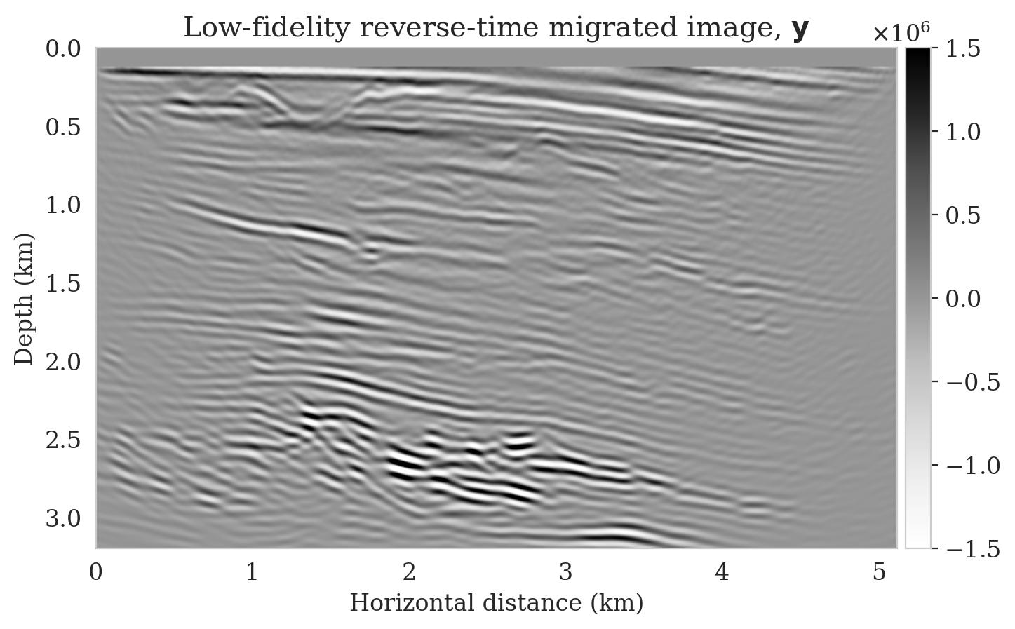
(b)

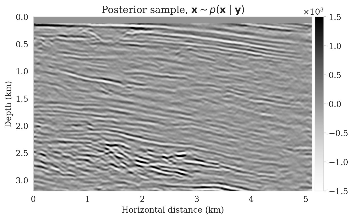
(c)

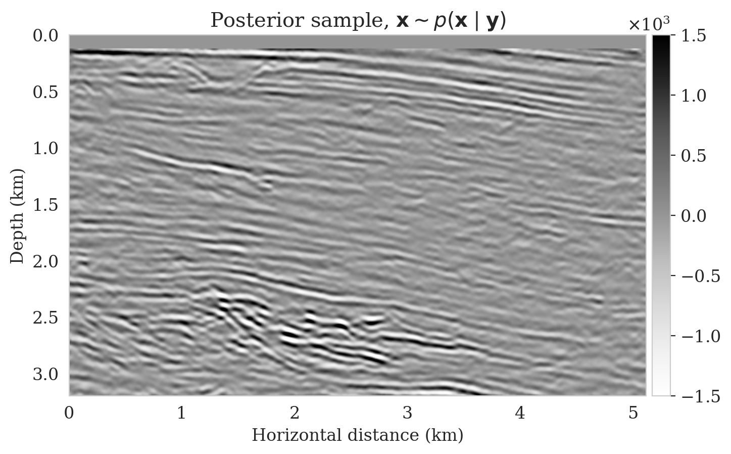
(d)

(e)

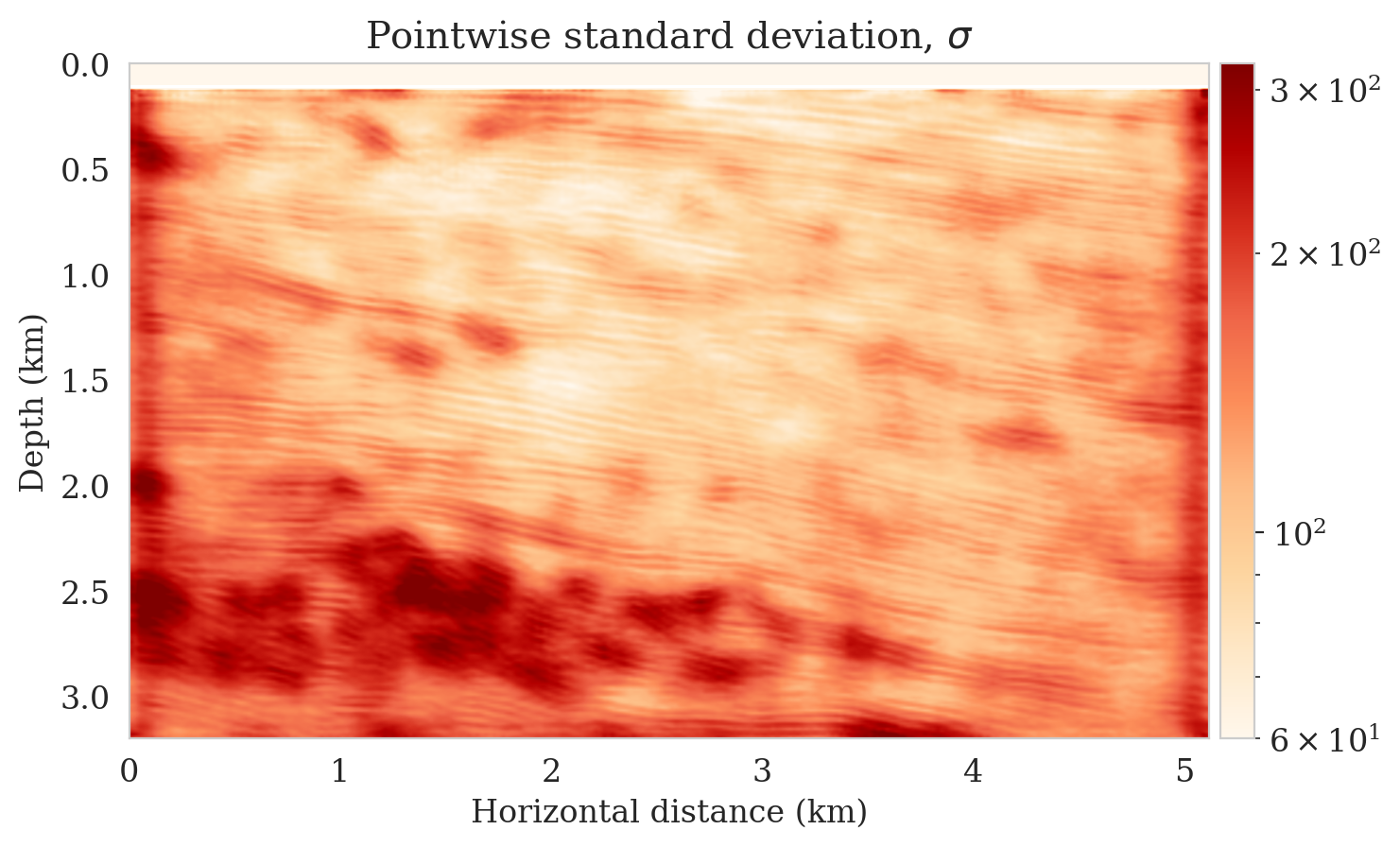
(f)

Figure 1: Reliability-aware imaging. (a) High-fidelity image. (b) Reverse-time migrated image. (c) and (d) Samples from posterior distribution. (e) Conditional mean and (f) pointwise standard deviation via the proposed method according to Equation 5.

In this example, we use Devito [43, 44] for the wave-equation based simulations. For implementation of the network architectures, we rely on InvertibleNetworks.jl [28], a memory-efficient framework for training invertible nets in the Julia programming language. Finally, code to reproduce our results are made available on https://github.com/slimgroup/Software.SEG2021.

4 Conclusions and discussion

Seismic imaging is challenging due to complex and computationally expensive-to-evaluate forward operators and the highly heterogeneous multiscale structure of the Earth. These challenges limit the applicability of Markov Chain sampling methods due to the costs associated with the forward operator. These difficulties are compounded by difficulties in capturing the heterogeneity exhibited by the Earth’s subsurface in the form of a prior distribution. To handle this situation and to assess uncertainty, we propose a data-driven, conditional normalizing-flow based variational inference approach. The proposed inference scheme takes advantage of having access to training pairs—e.g., in form of high-fidelity seismic images and low-fidelity remigrated images, to train a conditional normalizing flow capable of sampling from the posterior distribution. Because neural nets are known to generalize, the trained conditional normalizing flow can be used to quickly generate samples from the posterior given unseen low-fidelity images. In turn, these samples provide access to the high-fidelity conditional mean estimate including a rudimentary assessment of its uncertainty. In that sense, the presented imaging scheme learns by example, maximally leveraging what is already known. Since we can not completely rely on generalization of neural nets, the trained conditional normalizing flow can be used as input to a second physics-based stage of inference where the normalizing flow undergoes transfer learning and then samples from the posterior specific to the imaging problem at hand. By means of a numerical example, we demonstrate that our proposed scheme indeed provides fast access to posterior samples for problems that would otherwise be computationally unfeasible to solve with the more traditional methods. Since the presented method relies on generalization by conditional normalizing flows, we stop short of claiming that we quantify uncertainty but rather that we supply a measure of reliability of the estimated image.

5 Acknowledgment

This research was carried out with the support of Georgia Research Alliance and partners of the ML4Seismic Center.

References

- Tarantola [2005] Albert Tarantola. Inverse problem theory and methods for model parameter estimation. SIAM, 2005. ISBN 978-0-89871-572-9. doi: 10.1137/1.9780898717921.
- Robert and Casella [2004] C. Robert and G. Casella. Monte Carlo statistical methods. Springer-Verlag, 2004.
- Welling and Teh [2011] Max Welling and Yee Whye Teh. Bayesian Learning via Stochastic Gradient Langevin Dynamics. In Proceedings of the 28th International Conference on Machine Learning, ICML’11, pages 681–688, Madison, WI, USA, 2011. Omnipress. ISBN 9781450306195. doi: 10.5555/3104482.3104568. URL https://dl.acm.org/doi/abs/10.5555/3104482.3104568.
- Malinverno and Briggs [2004] Alberto Malinverno and Victoria A Briggs. Expanded uncertainty quantification in inverse problems: Hierarchical bayes and empirical bayes. GEOPHYSICS, 69(4):1005–1016, 2004. doi: 10.1190/1.1778243.
- Malinverno and Parker [2006] Alberto Malinverno and Robert L Parker. Two ways to quantify uncertainty in geophysical inverse problems. GEOPHYSICS, 71(3):W15–W27, 2006. doi: 10.1190/1.2194516.
- Martin et al. [2012] James Martin, Lucas C. Wilcox, Carsten Burstedde, and OMAR Ghattas. A Stochastic Newton MCMC Method for Large-scale Statistical Inverse Problems with Application to Seismic Inversion. SIAM Journal on Scientific Computing, 34(3):A1460–A1487, 2012. URL http://epubs.siam.org/doi/abs/10.1137/110845598.
- Ray et al. [2017] Anandaroop Ray, Sam Kaplan, John Washbourne, and Uwe Albertin. Low frequency full waveform seismic inversion within a tree based Bayesian framework. Geophysical Journal International, 212(1):522–542, 10 2017. ISSN 0956-540X. doi: 10.1093/gji/ggx428. URL https://doi.org/10.1093/gji/ggx428.
- Fang et al. [2018] Zhilong Fang, Curt Da Silva, Rachel Kuske, and Felix J. Herrmann. Uncertainty quantification for inverse problems with weak partial-differential-equation constraints. GEOPHYSICS, 83(6):R629–R647, 2018. doi: 10.1190/geo2017-0824.1.
- Stuart et al. [2019] Georgia K Stuart, Susan E Minkoff, and Felipe Pereira. A two-stage Markov chain Monte Carlo method for seismic inversion and uncertainty quantification. GEOPHYSICS, 84(6):R1003–R1020, 11 2019. doi: 10.1190/geo2018-0893.1.
- Zhao and Sen [2019] Zeyu Zhao and Mrinal K Sen. A gradient based MCMC method for FWI and uncertainty analysis. In SEG Technical Program Expanded Abstracts 2019, pages 1465–1469, 8 2019. doi: 10.1190/segam2019-3216560.1.
- Kotsi et al. [2020] M Kotsi, A Malcolm, and G Ely. Uncertainty quantification in time-lapse seismic imaging: a full-waveform approach. Geophysical Journal International, 222(2):1245–1263, 05 2020. ISSN 0956-540X. doi: 10.1093/gji/ggaa245.
- Curtis and Lomax [2001] Andrew Curtis and Anthony Lomax. Prior information, sampling distributions, and the curse of dimensionality. Geophysics, 66(2):372–378, 2001.
- Herrmann et al. [2019] Felix J. Herrmann, Ali Siahkoohi, and Gabrio Rizzuti. Learned imaging with constraints and uncertainty quantification. In Neural Information Processing Systems (NeurIPS) 2019 Deep Inverse Workshop, 12 2019. URL https://arxiv.org/pdf/1909.06473.pdf.
- Siahkoohi et al. [2020a] A. Siahkoohi, G. Rizzuti, and F. J. Herrmann. A deep-learning based bayesian approach to seismic imaging and uncertainty quantification. 82nd EAGE Conference and Exhibition 2020, 6 2020a. URL https://slim.gatech.edu/Publications/Public/Submitted/2020/siahkoohi2020EAGEdlb/siahkoohi2020EAGEdlb.html.
- Siahkoohi et al. [2020b] Ali Siahkoohi, Gabrio Rizzuti, and Felix J. Herrmann. Uncertainty quantification in imaging and automatic horizon tracking—a Bayesian deep-prior based approach. In SEG Technical Program Expanded Abstracts 2020, pages 1636–1640, 9 2020b. doi: 10.1190/segam2020-3417560.1.
- Jordan et al. [1999] Michael I Jordan, Zoubin Ghahramani, Tommi S Jaakkola, and Lawrence K Saul. An Introduction to Variational Methods for Graphical Models. Machine Learning, 37(2):183–233, 1999. doi: 10.1023/A:1007665907178.
- Blei et al. [2017] David M Blei, Alp Kucukelbir, and Jon D McAuliffe. Variational inference: A review for statisticians. Journal of the American statistical Association, 112(518):859–877, 2017.
- Rezende and Mohamed [2015] Danilo Rezende and Shakir Mohamed. Variational Inference with Normalizing Flows. In Proceedings of the 32nd International Conference on Machine Learning, volume 37 of Proceedings of Machine Learning Research, pages 1530–1538. PMLR, 07–09 Jul 2015. URL http://proceedings.mlr.press/v37/rezende15.html.
- Dinh et al. [2016] Laurent Dinh, Jascha Sohl-Dickstein, and Samy Bengio. Density estimation using Real NVP. arXiv preprint arXiv:1605.08803, 2016.
- Lensink et al. [2019] K. Lensink, E. Haber, and B. Peters. Fully Hyperbolic Convolutional Neural Networks, 2019.
- Kruse et al. [2019] Jakob Kruse, Gianluca Detommaso, Robert Scheichl, and Ullrich Köthe. HINT: Hierarchical Invertible Neural Transport for Density Estimation and Bayesian Inference. arXiv preprint arXiv:1905.10687, 2019.
- Goodfellow et al. [2014] Ian Goodfellow, Jean Pouget-Abadie, Mehdi Mirza, Bing Xu, David Warde-Farley, Sherjil Ozair, Aaron Courville, and Yoshua Bengio. Generative Adversarial Nets. In Proceedings of the 27th International Conference on Neural Information Processing Systems, NIPS’14, pages 2672–2680, 2014. URL http://papers.nips.cc/paper/5423-generative-adversarial-nets.pdf.
- Mosser et al. [2020] Lukas Mosser, Olivier Dubrule, and Martin J. Blunt. Stochastic seismic waveform inversion using generative adversarial networks as a geological prior. Mathematical Geosciences, 52(1):53–79, 2020. doi: 10.1007/s11004-019-09832-6. URL https://doi.org/10.1007/s11004-019-09832-6.
- Bishop [2006] Christopher M Bishop. Pattern Recognition and Machine Learning. Springer-Verlag New York, 2006.
- Arjovsky et al. [2017] Martin Arjovsky, Soumith Chintala, and Léon Bottou. Wasserstein generative adversarial networks. In Proceedings of the 34th International Conference on Machine Learning, volume 70 of Proceedings of Machine Learning Research, pages 214–223. PMLR, 06–11 Aug 2017. URL http://proceedings.mlr.press/v70/arjovsky17a.html.
- Putzky and Welling [2019] Patrick Putzky and Max Welling. Invert to learn to invert. In H. Wallach, H. Larochelle, A. Beygelzimer, F. d'Alché-Buc, E. Fox, and R. Garnett, editors, Advances in Neural Information Processing Systems, volume 32. Curran Associates, Inc., 2019. URL https://proceedings.neurips.cc/paper/2019/file/ac1dd209cbcc5e5d1c6e28598e8cbbe8-Paper.pdf.
- Peters and Haber [2020] Bas Peters and Eldad Haber. Fully reversible neural networks for large-scale 3d seismic horizon tracking. In 82nd EAGE Annual Conference & Exhibition, pages 1–5. European Association of Geoscientists & Engineers, 2020.
- Witte et al. [2021] Philipp Witte, Gabrio Rizzuti, Mathias Louboutin, Ali Siahkoohi, Felix Herrmann, and Bas Peters. InvertibleNetworks.jl: A Julia framework for invertible neural networks, March 2021. URL https://doi.org/10.5281/zenodo.4610118.
- WesternGeco. [2012] WesternGeco. Parihaka 3D PSTM Final Processing Report. Technical Report New Zealand Petroleum Report 4582, New Zealand Petroleum & Minerals, Wellington, 2012.
- Liu [2017] Qiang Liu. Stein variational gradient descent as gradient flow. In I. Guyon, U. V. Luxburg, S. Bengio, H. Wallach, R. Fergus, S. Vishwanathan, and R. Garnett, editors, Advances in Neural Information Processing Systems, volume 30. Curran Associates, Inc., 2017. URL https://proceedings.neurips.cc/paper/2017/file/17ed8abedc255908be746d245e50263a-Paper.pdf.
- Zhang and Curtis [2020a] Xin Zhang and Andrew Curtis. Seismic tomography using variational inference methods. Journal of Geophysical Research: Solid Earth, 125(4):e2019JB018589, 2020a.
- Zhang and Curtis [2020b] Xin Zhang and Andrew Curtis. Variational full-waveform inversion. Geophysical Journal International, 222(1):406–411, 04 2020b. ISSN 0956-540X. doi: 10.1093/gji/ggaa170. URL https://doi.org/10.1093/gji/ggaa170.
- Rizzuti et al. [2020] Gabrio Rizzuti, Ali Siahkoohi, Philipp A. Witte, and Felix J. Herrmann. Parameterizing uncertainty by deep invertible networks, an application to reservoir characterization. In SEG Technical Program Expanded Abstracts, pages 1541–1545, 09 2020. doi: 10.1190/segam2020-3428150.1.
- Zhao et al. [2020] Xuebin Zhao, Andrew Curtis, and Xin Zhang. Bayesian seismic tomography using normalizing flows. 2020. doi: 10.31223/X53K6G. URL https://eartharxiv.org/repository/view/1940/.
- Siahkoohi et al. [2021] Ali Siahkoohi, Gabrio Rizzuti, Mathias Louboutin, Philipp Witte, and Felix J. Herrmann. Preconditioned training of normalizing flows for variational inference in inverse problems. In 3rd Symposium on Advances in Approximate Bayesian Inference, 1 2021. URL https://openreview.net/pdf?id=P9m1sMaNQ8T.
- Siahkoohi et al. [2020c] Ali Siahkoohi, Gabrio Rizzuti, Philipp A. Witte, and Felix J. Herrmann. Faster uncertainty quantification for inverse problems with conditional normalizing flows. Technical Report TR-CSE-2020-2, Georgia Institute of Technology, 07 2020c. URL https://arxiv.org/abs/2007.07985.
- Adler and Öktem [2018] Jonas Adler and Ozan Öktem. Deep Bayesian Inversion. arXiv preprint arXiv:1811.05910, 2018.
- Kovachki et al. [2020] Nikola Kovachki, Ricardo Baptista, Bamdad Hosseini, and Youssef Marzouk. Conditional Sampling With Monotone GANs. arXiv preprint arXiv:2006.06755, 2020.
- Villani [2009] Cédric Villani. Optimal transport: old and new. Springer-Verlag Berlin Heidelberg, 2009. doi: 10.1007/978-3-540-71050-9.
- Marzouk et al. [2016] Youssef Marzouk, Tarek Moselhy, Matthew Parno, and Alessio Spantini. Sampling via measure transport: An introduction. Handbook of uncertainty quantification, pages 1–41, 2016.
- Kingma and Ba [2014] Diederik P. Kingma and Jimmy Ba. Adam: A Method for Stochastic Optimization. CoRR, abs/1412.6980, 2014.
- Anderson and Moore [1979] Brian D.O. Anderson and John B. Moore. Optimal Filtering. Prentice-Hall, Englewood Cliffs, NJ., 1979.
- Luporini et al. [2018] F. Luporini, M. Lange, M. Louboutin, N. Kukreja, J. Hückelheim, C. Yount, P. Witte, P. H. J. Kelly, F. J. Herrmann, and G. J. Gorman. Architecture and performance of devito, a system for automated stencil computation. CoRR, abs/1807.03032, jul 2018. URL http://arxiv.org/abs/1807.03032.
- Louboutin et al. [2019] M. Louboutin, M. Lange, F. Luporini, N. Kukreja, P. A. Witte, F. J. Herrmann, P. Velesko, and G. J. Gorman. Devito (v3.1.0): an embedded domain-specific language for finite differences and geophysical exploration. Geoscientific Model Development, 12(3):1165–1187, 2019. doi: 10.5194/gmd-12-1165-2019. URL https://www.geosci-model-dev.net/12/1165/2019/.