Laminar and Turbulent Plasmoid Ejection in a Laboratory Parker Spiral Current Sheet

Abstract

Quasi-periodic plasmoid formation at the tip of magnetic streamer structures is observed to occur in experiments on the Big Red Ball as well as in simulations of these experiments performed with the extended-MHD code, NIMROD. This plasmoid formation is found to occur on a characteristic timescale dependent on pressure gradients and magnetic curvature in both experiment and simulation. Single mode, or laminar, plasmoids exist when the pressure gradient is modest, but give way to turbulent plasmoid ejection when the system drive is higher, producing plasmoids of many sizes. However, a critical pressure gradient is also observed, below which plasmoids are never formed. A simple heuristic model of this plasmoid formation process is presented and suggested to be a consequence of a dynamic loss of equilibrium in the high-$\beta$ region of the helmet streamer. This model is capable of explaining the periodicity of plasmoids observed in the experiment and simulations and produces plasmoid periods of 90 minutes when applied to 2D models of solar streamers with a height of $3R_{\odot}$. This is consistent with the location and frequency at which periodic plasma blobs have been observed to form by LASCO and SECCHI instruments.

1 Introduction

Over the past few decades, in-situ measurements of the solar wind have produced an enormous amount of data that can be used to characterize properties of the solar wind and to discover its source regions on the Sun. One of the earliest characterizations was the observation of “fast” and “slow” streams of wind as measured by Mariner II (Neugebauer & Snyder, 1962). However, later on it was discovered that the slow wind was better characterized by the charge state ratios of oxygen — indicating a much higher electron temperature in the source region (Neugebauer et al., 2016; Fu et al., 2017; Cranmer et al., 2017), consistent with the temperatures and charge states in well confined coronal loops. This led to the understanding that the slow solar wind likely originates from transport between closed flux and open flux in the equatorial streamer belt and that it can only occur via magnetic reconnection. This formation process is drastically more complex than the fast wind acceleration in coronal holes, which agrees with the original Parker solution (Parker, 1958) and produces a relatively quiescent, supersonic flow with photospheric abundances. Invoking magnetic reconnection in the formation mechanism of the slow wind inherently leads to a dynamic process capable of explaining its high degree of variability. However, spontaneous magnetic reconnection is difficult to achieve in high Lundquist number plasmas and so a mechanism with enough free energy for facilitating or driving the reconnection must be included in the theory. To this end, a number of theories have been postulated including “interchange reconnection” (Crooker et al., 2000; Fisk et al., 1998; Fisk, 2003), the S-Web theory (Antiochos et al., 2011; Higginson & Lynch, 2018; Antiochos et al., 2007), and streamer top reconnection (Einaudi et al., 2001, 1999; Lapenta & Knoll, 2005; Endeve et al., 2004; Wu et al., 2000).

Specifically with regards to streamer top reconnection, a number of computational studies have attempted to recreate these periodic density structures (PDSs). This process can be driven by instabilities in the coronal loop or by converging flows at the streamer cusp (Einaudi et al., 2001, 1999; Lapenta & Knoll, 2005; Wu et al., 2000) and has also revealed that two-fluid effects can alter plasmoid characteristics emanating from helmet streamers (Endeve et al., 2003, 2004). These multi-fluid simulations prescribe a fixed amount of coronal heating at the base of the helmet streamer, which results in a dynamic system with no equilibrium that oscillates periodically. However, the periodicity of the plasmoids in these simulations is longer than that observed, $\sim$15-20 hours.

With the improvements to imaging diagnostics on many of the current satellite missions (SOHO, STEREO, Parker Solar Probe), as well as novel data analysis techniques, increasingly smaller and more dynamic features are constantly being revealed in the solar wind (DeForest et al., 2018; Bale et al., 2019). One example of this pertains specifically to the slow solar wind and the observation of PDSs, also known as plasma blobs or plasmoids, that are released into the solar wind at the tips of helmet streamers (Wang et al., 1997; Sheeley, Jr. et al., 1997; Lavraud et al., 2020). Running difference calculations of white light images produced by SOHO’s Large Angle and Spectrometric Coronograph (LASCO) (Brueckner et al., 1995) reveal bipolar signatures indicative of small scale structures propagating outwards into the solar wind (Wang et al., 1998). Recently these PDSs have also been identified by the SECCHI instrument suite onboard STEREO (Viall & Vourlidas, 2015), in old Helios data (Di Matteo et al., 2019), and during Parker Solar Probe’s first orbit (Lavraud et al., 2020). They have also been observed to have magnetic signatures (Rouillard et al., 2011) and be the product of magnetic reconnection at the open-closed flux boundary of helmet streamers (Kepko et al., 2016; Sanchez-Diaz et al., 2019).

While the work of Viall & Vourlidas (2015) shows that blobs form at or below $2.5R_{\odot}$ and have a typical period of 90 minutes with a range of 65-100 minutes, other work suggests that blobs can also form at larger radii ($2-6R_{\odot}$) and have longer periods of a few hours (Wang & Hess, 2018; Wang et al., 1998). The implied correlation between these observations is that when helmet streamer tips are closer to the Sun they release higher frequency PDSs, and lower frequency PDSs when they are further away. This hypothesis is consistent with the observations of a wide number of variable discrete frequencies that are observed in the slow solar wind at 1AU over the course of the solar cycle (Viall et al., 2008).

Aside from the presence of multiple coherent frequencies of observed PDSs, it is also well understood that the heliospheric current sheet (HCS) — and the solar wind as a whole — is extremely turbulent (Bavassano et al., 1997; Coleman et al., 1968; Bavassano & Bruno, 1989a, b; Luttrell & Richter, 1987; Belcher & Davis, 1971; Marsch & Tu, 1990a, b; Bale et al., 2019) and evolves as a function of distance from the Sun (Bavassano et al., 1982). Even though fully developed turbulence is typically observed to exist by $0.3R_{\odot}$ in the slow wind near the HCS, it is often not enough to completely decorrelate the coherent PDS fluctuations generated in the corona as they are routinely observed to drive magnetospheric fluctuations at 1AU (Viall et al., 2008; Kepko et al., 2002; Stephenson & Walker, 2002; Kepko & Spence, 2003).

The conclusion from this plethora of observational insight is that any mesoscale model that wishes to accurately describe the acceleration of the solar wind near the magnetic equator must be able to produce these coherent fluctuations embedded in a turbulent background that evolves as it travels away from the source. It is also necessary that the frequencies be on the proper time scales and that the fluctuations are consistent with density and magnetic signatures indicative of plasmoids.

In this article we report on experimental observations of axisymmetric plasmoid ejection via helmet streamer tip reconnection in a laboratory Parker Spiral. We discuss a potential plasmoid formation mechanism and observations of plasmoid scaling properties by comparisons between experimental measurements and extended-MHD simulations performed with the two-fluid modeling capabilities of the NIMROD code (Sovinec et al., 2004; Sovinec & King, 2010). These scalings indicate higher frequency plasmoids for more elongated streamers with thinner current sheets, as well as an evolution toward turbulence further downstream as plasmoids of many sizes interact. Lastly, a simple heuristic model is presented suggesting that the periodicity of plasmoids in the experiments and simulations and those produced in the solar wind is set by a dynamic transition from a state of quasi-equilibrium to one where no such equilibrium exists — a process we will refer to as equilibrium loss. It is important to note that the helmet streamers produced in the lab and those in the solar wind represent drastically different systems; the former is governed by Hall-MHD and exists on sub-ion scales, whereas the latter is much better described by ideal MHD and exists on scales much, much larger than any kinetic scale. This article does not make any claims about the relationship of the dominant transport mechanisms between the two systems, nor does it claim that the underlying physics of the subsequent reconnection events are the same. The simple association is made that both systems exhibit sonic outflows that result in periodic plasmoid ejection from the tip of the helmet streamers and that the loss of equilibrium responsible for this phenomenon can be driven by pressure gradients and magnetic curvature both in the experiments and in the solar wind.

2 Experimental and Simulation Methodologies

The Big Red Ball (BRB) at the Wisconsin Plasma Physics Laboratory is a versatile plasma confinement device well-suited to the study of high-$\beta$ and flow-dominated systems. The capabilities of the BRB are discussed in more detail in other works (Forest et al., 2015; Olson et al., 2016; Flanagan et al., 2020; Endrizzi et al., 2021) and the experimental setup of the Parker Spiral solar wind experiments and initial findings are detailed in Peterson et al. (2019). A depiction of the experimental configuration of the BRB for these experiments as well as the computational model of the experiment are shown in Fig. 1. The summary of the experimental methodology for generating the Parker Spiral in the BRB is as follows: Thermally emissive Lanthanum-Hexaboride cathodes are used to generate a warm, dense, unmagnetized plasma atmosphere ($T_{e}\sim 7$ eV, $n_{e}\sim 4\times 10^{17}$ m^-3). A permanent dipole magnet is placed inside this background plasma with two ring electrodes located near its north and south poles. Current is driven from molybdenum anodes in the plasma atmosphere into the dipole magnetosphere and collected on the polar electrodes. This current path is visualized in Fig. 1(b) in the context of the NIMROD simulation domain. These cross field currents generate a torque on the plasma which causes the magnetosphere to rotate, thereby twisting the magnetic field into a Parker Spiral.

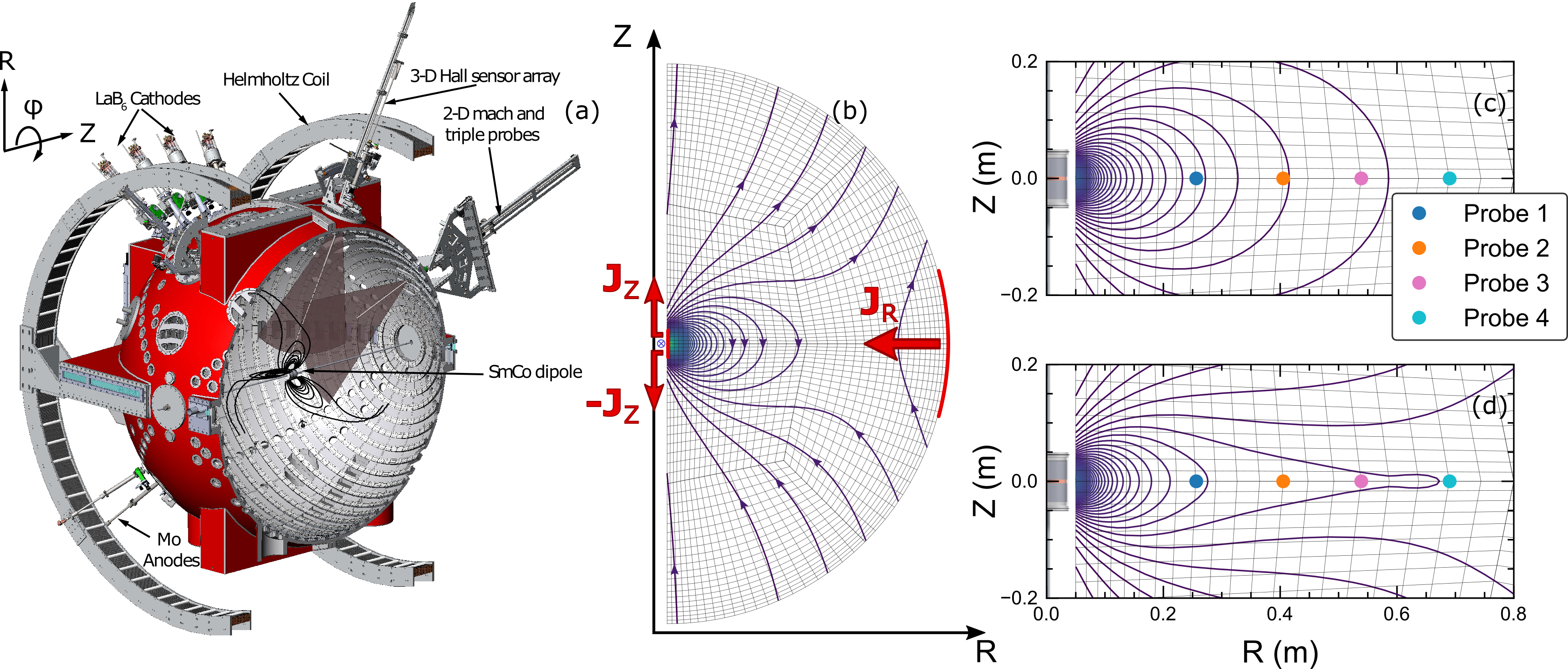
Figure 1: Experimental (a) and computational (b, c, d) configurations. The Big Red Ball is shown in (a) along with the local cylindrical coordinate system, dipole magnet, and diagnostics used for mapping the magnetosphere. The 2D finite element mesh with current injection boundary conditions and initial vacuum field configuration are shown in (b). Panels (c) and (d) show the location of probes within the NIMROD simulation for outputting high time resolution field measurements. Both the initial magnetic field configuration (c) and time-averaged magnetic field configuration after the current injection has reached steady state (d) are shown to demonstrate the probe positions relative to where the plasmoid formation process occurs.

At the interface between the closed field lines of the magnetosphere and the open field lines of the Parker Spiral, periodic reconnection occurs, ejecting axisymmetric plasmoids, much like the density structures observed in the heliospheric current sheet which emanate from streamer top reconnection. A number of diagnostics were employed to map the 2D time dynamics of the Parker Spiral including two arrays of 3 axis Hall sensors and an array of triple probes and 2D Mach probes for measuring density, temperature, and flows in the plasma. One of the Hall sensor arrays was kept stationary and displaced azimuthally from the 2D scanning plane to provide phase reference measurements critical for the reconstruction of the plasmoid dynamics.

The computational domain and vacuum magnetic field for the accompanying NIMROD simulations are shown in Fig. 1. Figure 1(b) represents the hemispherical mesh in cylindrical coordinates, which extends down to $R=5$ cm rather than the experiment’s support rod at $R=2$ cm. This is to allow for a small dipole magnet to be placed outside the computational domain and to facilitate the boundary condition manipulation to model current injection/extraction in a manner representative of the experiment. By prescribing $B_{\varphi}$ along the boundary as a function of time, we can set the normal component of $J$, or the current into and out of the vessel. In all the presented simulation work that follows, the current injection linearly ramps from zero up to a prescribed steady state value. The ramp duration in some of the initial simulations was 1 ms, but was shortened to 100 $\mu$s to reduce the required simulation time for some of the higher current injection cases that have smaller time steps. For all simulations discussed in this work, there are zero heat flux and zero particle flux conditions applied to the boundary as well as a no-slip boundary condition on the velocity. All simulations were performed with experimental parameters of $n_{\mathrm{e}}=4\times 10^{17}$ m^-3, $T_{\mathrm{e}}=7$ eV, $T_{\mathrm{i}}=0.5$ eV, which give viscous and resistive diffusivities of $\nu=50$ m${}^{2}/$s and $\eta=35$ m${}^{2}/$s respectively. We also note that in the experiments and simulations the ion skin depth is set to $d_{i}=70$ cm. In terms of resolution, the simulations were performed with 2400 bicubic poloidal elements which provides centimeter-scale resolution in the current sheet.

In order to better compare results from simulation to the experimental measurements, the NIMROD code was modified in order to take a list of R, Z coordinates for placing history nodes, or probes. For the simulations in this study, four probes were placed in the current sheet at $R=25,40,55,70$ cm and $Z=0$ cm as shown in Fig. 1. The probe locations relative to the vacuum magnetic flux configuration and the flux distribution near the end of a simulation can be seen in Fig. 1(c) and Fig. 1(d) respectively. These probes provide outputs for the solution fields after every time step to allow for higher frequency phenomena to still be captured at a few select locations in the simulation. All NIMROD simulations presented in this work are axisymmetric.

3 Observation of Streamer Top Reconnection and Plasmoid Formation in Experiment and Two-Fluid Simulations

While the basic operating parameters, mean magnetic field, and plasma flows that develop in both the experiment and simulations are presented in Peterson et al. (2019), this article sheds more light on the details of the fluctuation measurements as well as their scaling properties. Previous work demonstrated that, during the generation of the Parker Spiral, two fluid effects are critical as the system size is small compared to the ion skin depth, the electrons are the only magnetized species, and $T_{e}\gg T_{i}$. The consequence of this is a radially outward flow of electrons that advects the dipolar magnetic field into a Parker Spiral and simultaneously generates an inward electric field via the Hall effect. This Hall electric field drives accretion of ions into the magnetosphere where a density and pressure gradient begin to build until a loss of equilibrium occurs. In both experiment and simulation, this loss of equilibrium occurs in the current sheet associated with the Parker Spiral where $\beta>10$ (Peterson et al., 2019) and increases up to $\beta\sim 50$ further downstream.

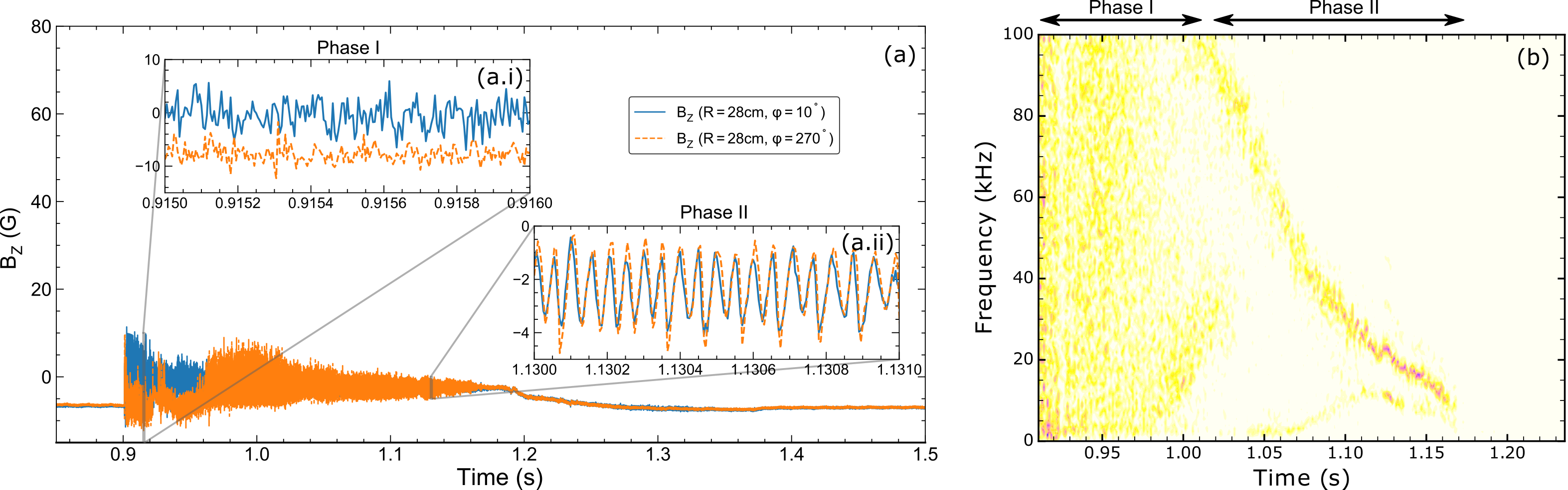
Figure 2: Time histories and frequency content of magnetic signals measured in the Parker Spiral current sheet by 3-axis Hall sensors in the experiment. The difference between the turbulent, non-axisymmetric Phase I and axisymmetric, single mode Phase II can be seen in (a) where two probes at the same radius, but different azimuthal angles have very different mean field values as well as high frequency characteristics in (a.i.), but are nearly identical in Phase II (a.ii). A spectrogram of one of these time histories (b) shows broadband fluctuations in Phase I, followed by a coherent downward chirping spectrum of laminar plasmoid ejection.

Measurements of the magnetic field as well as the plasma density show interesting fluctuations whose frequency depends on the amount of current injected. As shown in Fig. 2(a), the vertical component of the magnetic field, $B_{Z}$ (the poloidal component perpendicular to the current sheet) is non-axisymmetric and highly uncorrelated in the initial, high current phase of the experiment (Phase I). However, as shown in Fig. 2(a.ii), these magnetic fluctuations become coherent as the current injection falls with the characteristic timescale set by the RC circuit of the current injection system ($\sim 100$ms). In addition, the $B_{Z}$ fluctuations are bi-polar and thus suggestive of closed loops of magnetic flux disconnected from the inner magnetosphere of the rotating plasma. A spectrogram typical of these magnetic fluctuations in the current sheet can be seen in Fig. 2(b) which shows the turbulent nature of the high current Phase I and coherent mode Phase II with a high degree of correlation between the plasmoid frequency and current injection of the system. This scaling relationship will be discussed in subsequent sections.

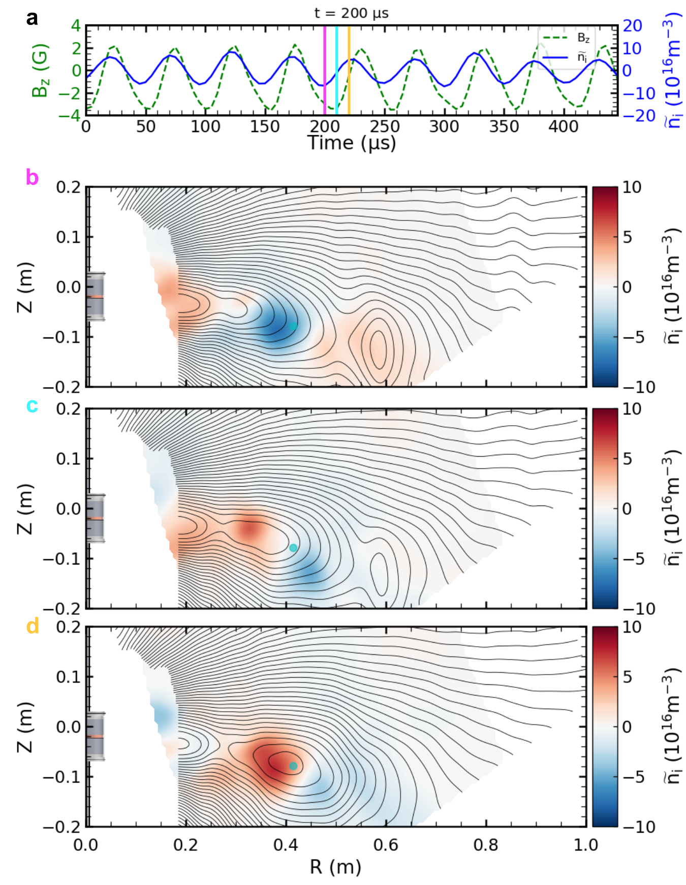
Figure 3: Plasmoids are ejected from the helmet streamer cusp at a frequency of 20 kHz when the current injection is 150 A in the experiment. Panel (a) shows the magnetic field ($B_{Z}$) and density fluctuation ($\tilde{n}_{i}$) signals as measured by the probe in the current sheet at $R=42$ cm and denoted by the teal dot in panels (b), (c), and (d). Panels (b), (c), and (d) show the flux map and density perturbation map at three successive 10 $\mu$s time steps corresponding to the magenta, cyan, and yellow vertical lines in (a). These panels show how the magnetic field at the streamer cusp expands outwards with higher density plasma until reconnection occurs, releasing a plasmoid into the current sheet.

Performing phase correlation measurements between the stationary Hall array and the scanning array over many discharges allows us to reconstruct the plasmoid dynamics — both magnetic field and density — through conditional averaging. This reconstruction method first identifies 500 $\mu$s time windows for every shot that exhibit the highest degree of shot-to-shot similarity as measured by a single stationary hall probe. A center frequency of 20 kHz was used for this process as it showed the best correlation shot-to-shot between 1.1 and 1.15 seconds as shown in Fig. 2(b). Once the best time window from each shot is selected, a phase shift is calculated for each shot using the stationary reference probe which allows us to align in time the many different shots at different locations and build up a poloidal map of the 2D plasma dynamics. This process reveals periodic reconnection occurring near the top of the streamer structures resulting in plasmoids being ejected into the Parker spiral current sheet as shown in Fig. 3. Figure 3(a) shows the $B_{Z}$ measurement as well as ion density fluctuations $\tilde{n}_{i}$ as measured by the probe located at ($R=42$cm, $Z=-8$cm) and shown as a cyan dot in Fig. 3(b-d). We believe the up-down asymmetry of the current sheet, or “droop”, is likely due to preferential current draw to an anode in the southern hemisphere that was larger than the others, which is not captured in simulations since the current injection is uniform over the range of $\pm 15^{\circ}$ latitude. Figure 3(b-d) show subsequent time steps of 10$\mu$s through one half period of the reconnection process, which exhibits a periodic build up of plasma density (and pressure) inside the streamer leading to field line stretching, reconnection, and plasmoid ejection.

In addition to plasmoids observed experimentally, they also manifest in extended MHD simulations when the Hall term and electron pressure gradient term are used in Ohm’s law. 2D cross sections of the magnetic flux and density fluctuations from the NIMROD simulations as well as the time resolved signals in the current sheet as would be measured by probes in the experiment or satellites in space are shown in Fig. 4 and Fig. 5. The time histories of both experimental and laminar plasmoids can be seen in movies published in previous work (Peterson et al., 2019), whereas the evolution of the turbulent plasmoids in Fig. 5 can be viewed in the movie turbulent_plasmoids.mp4. Figure 4 represents a moderate current injection level of 400 A in the simulation which is slightly above the threshold necessary to observe plasmoids. As a result, we observe relatively large single plasmoids emitted with a very regular frequency. We refer to these plasmoids as laminar since the magnetic flux evolves very smoothly with regular ejection of similarly sized plasmoids.

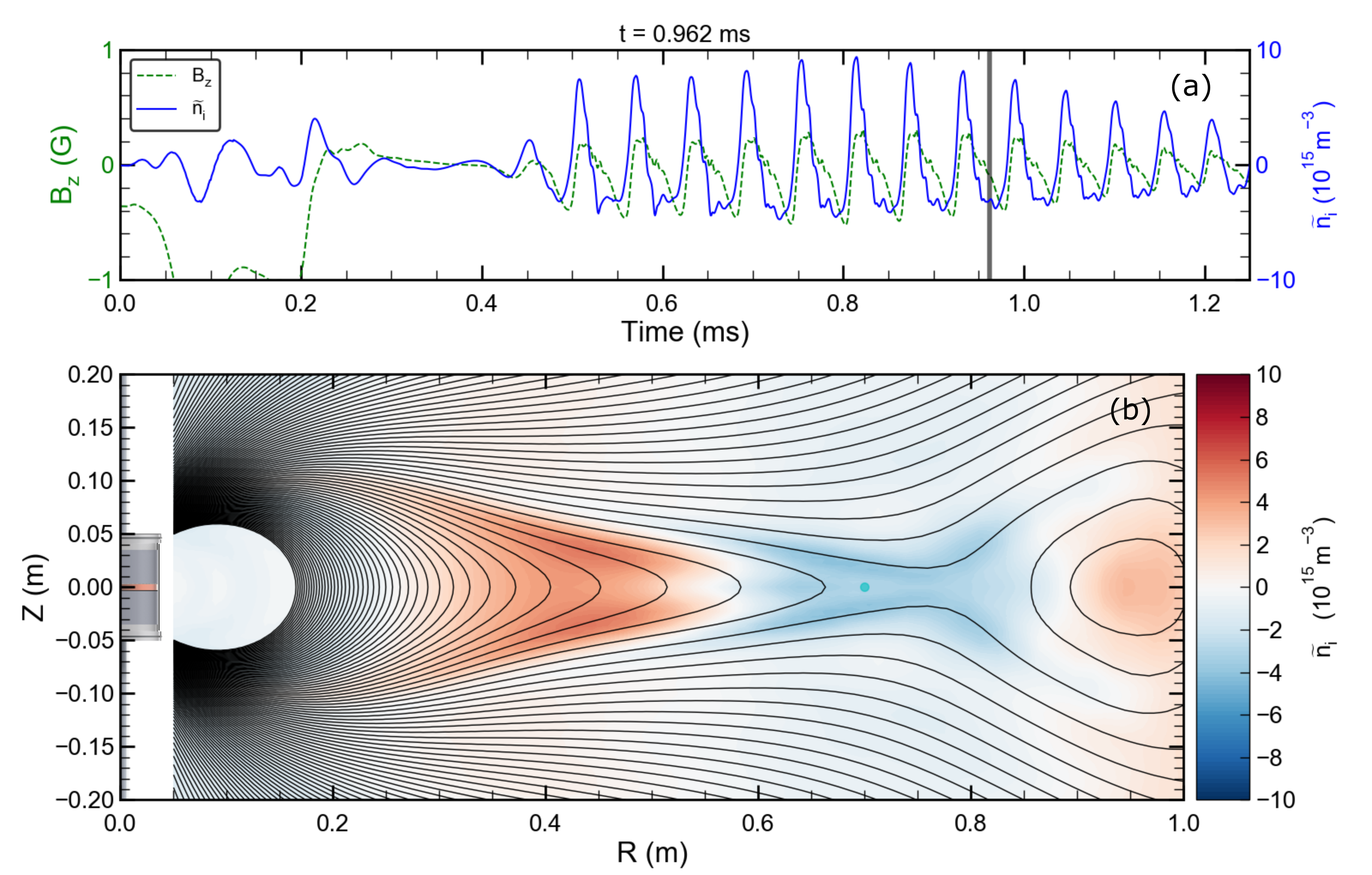
Figure 4: Laminar plasmoid formation in an axisymmetric NIMROD simulation with 400A of injected current. The time history of $B_{Z}$ and ion density fluctuations as measured by a probe at $R=70$cm (top panel) shows the periodic ejection of high density plasmoids that are roughly similar size over time.

On the other hand, Fig. 5 represents a high current drive case of 1000 A where we see plasmoids of many sizes interacting in a thinner current sheet resulting in a more turbulent medium downstream.

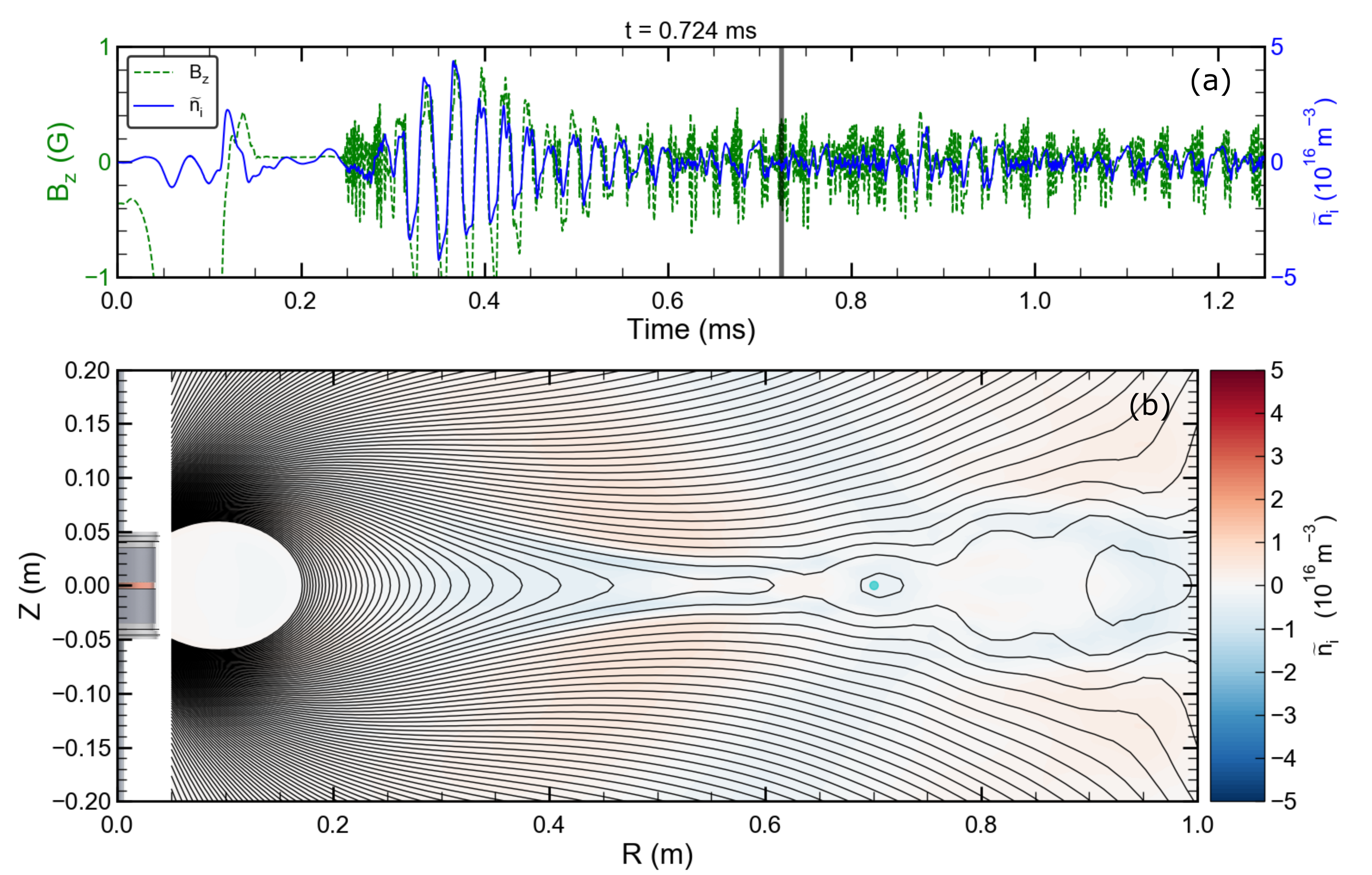
Figure 5: Turbulent plasmoid formation in an axisymmetric NIMROD simulation with 1000A of injected current. The time history of $B_{Z}$ and ion density fluctuations as measured by a probe at $R=70$cm (top panel) shows the high variability of plasmoids in both frequency and size.

The observation of plasmoids in the experiment as well as in the NIMROD simulations begs the question of whether this occurrence is coincidence or if the same physical processes are driving plasmoid formation in both cases. Importantly, theoretical and computational studies (Bhat & Loureiro, 2018), as well as experiments (Hare et al., 2017) have demonstrated that plasmoid formation can occur at values of the Lundquist number much below the usual $10^{4}$ required in resistive MHD when ion-scale kinetic effects are not negligible, as is the case here. We now turn our attention to a discussion of the properties and scaling relationships for these observed plasmoids.

4 Discussion of Laminar and Turbulent Plasmoid Formation, Properties, and Scalings

We begin by discussing the characteristics of these plasmoids, particularly with respect to the amount of current injected into the experiment (or simulation). Shown in Fig. 6 are the time-averaged magnetic field configurations in the simulations (a-c) and experiment (d-f) as a function of increasing current injection. As more flux is advected outwards with the electron flow, it results in a current sheet thinning effect as shown in Fig. 6, where the thinner current sheets display larger magnetic curvature near the streamer cusp. As shown in both Fig. 7 and Fig. 8, these elongated streamers associated with higher current injection values result in higher frequency plasmoid ejection. However, plasmoids are not present for every current injection value in the simulation and experiment. This is shown in Fig. 7 which shows $B_{Z}$ power spectral densities from four different simulations with increasing amounts of current injection: 200A, 400A, 600A, and 1000A for panels (a), (b), (c), and (d), respectively. We can see that no plasmoids are present in the 200A simulation, likely because the accretion caused by the Hall effect is not strong enough to build up pressure above the critical gradient necessary for loss of equilibrium.

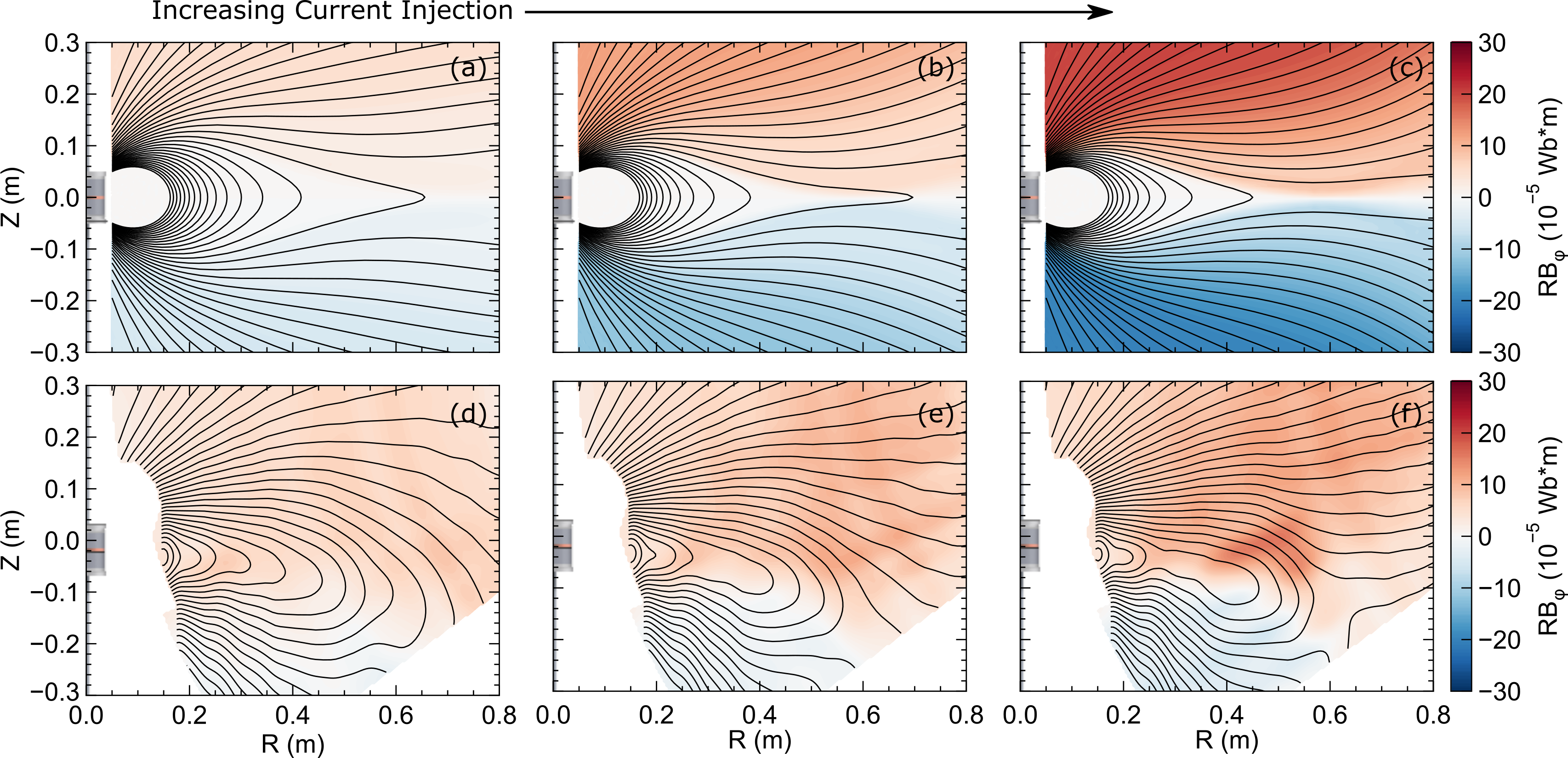
Figure 6: Mean-field evolution of the magnetic field as a function of current injection is shown for axisymmetric NIMROD simulations (a-c) as well as the experiment (d-f). The top row depicts both the time-averaged poloidal and toroidal magnetic field at three different current injection values: 250 A, 600 A, and 1000 A, from left to right, respectively. In this progression, it is clear that the current sheet becomes thinner and the toroidal magnetic field increases as the poloidally injected current is increased. The same is true in the experiment as shown in the bottom row, where the current injection values are 150 A, 250 A and 350 A, respectively. For currents larger than 350 A in the experiment, the magnetic field is highly non-axisymmetric; as a result, axisymmetric flux surface reconstruction is not possible.

Another characteristic that trends with increased system drive (or current injection) is a decrease in coherence of the fluctuations and increase in turbulence. In Fig. 7(b) we can see a well defined fundamental frequency at 15 kHz as well as multiple resolved harmonics. However, as the current is increased in panels (c) and (d), the spectra become more broadband and the fundamental mode increases in frequency, which is consistent with the experimental observations reported in Peterson et al. (2019).

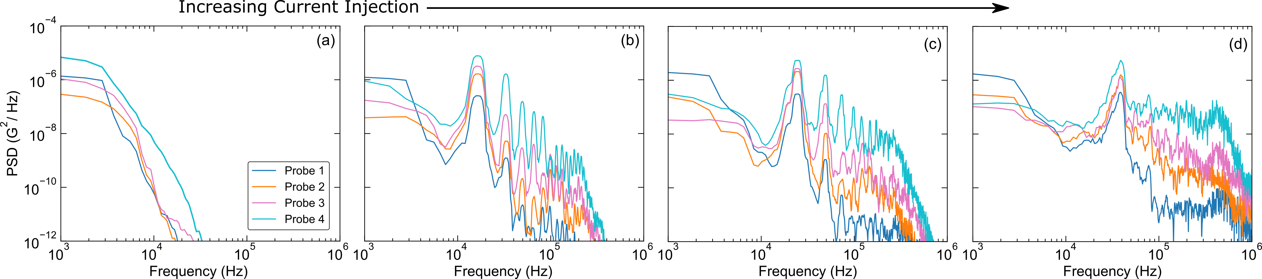
Figure 7: $B_{Z}$ fluctuation power spectra from four probes in four different two-fluid NIMROD simulations with current values of 200A, 400A, 600A, and 1000A shown in panels (a), (b), (c), and (d), respectively. Probes 1-4 are located at increasing radii in the current sheet as according to Fig. 1. Increasing the injected current increases both the fundamental plasmoid frequency as well as the amplitudes of higher frequency components. Fluctuations are increasingly more broadband at larger radial distances as well.

One more important observation from Fig. 7 is that field lines at inner radii (closer to probe 1) are more coherent — that is, the dominant mode is much stronger relative to the other higher frequencies. The physical interpretation of this phenomenon is that the pressure inside the magnetosphere drives a periodic loss of equilibrium that manifests as magnetospheric oscillations that drive larger fluctuations further out in the current sheet where the field is weaker, ultimately resulting in a turbulent current sheet that still has a quasi-periodic nature.

A comparison of the plasmoid frequencies in simulation to those observed in the experiment is shown in Fig. 8(a) as a function of current (orange and green triangles). In Fig. 8(a) each experimental data point represents the peak value in the $B_{Z}$ frequency spectrum from a single Hall probe in 10 ms windows between 0.9 and 1.4 seconds. This generates 50 data points per shot and is plotted for roughly 100 shots. The simulation results (blue circles) show the dominant frequency for the duration of the simulation once the current injection has reached steady state. Each data point for the NIMROD simulations therefore represents a single simulation at a single current injection value. It is important to note the strong linear scaling at modest current injection up to $\sim 400$ A, as well as the abrupt disappearance of plasmoids below 100 A and $\sim 10$ kHz. The high density of data points at very low frequency for currents above $\sim 300$ A, are not particularly germane to this discussion and just indicate that the frequency range with the highest power spectral density was found to be at low frequencies during the non-axisymmetric phase of the experiment and can be seen as well in the Phase II portion of the spectrogram in Fig. 2(b). Also plotted is the fundamental plasmoid frequency from the Hall-MHD NIMROD simulations as a function of current. Both experimental and simulation plasmoid frequencies scale linearly with the current, but with different slopes.

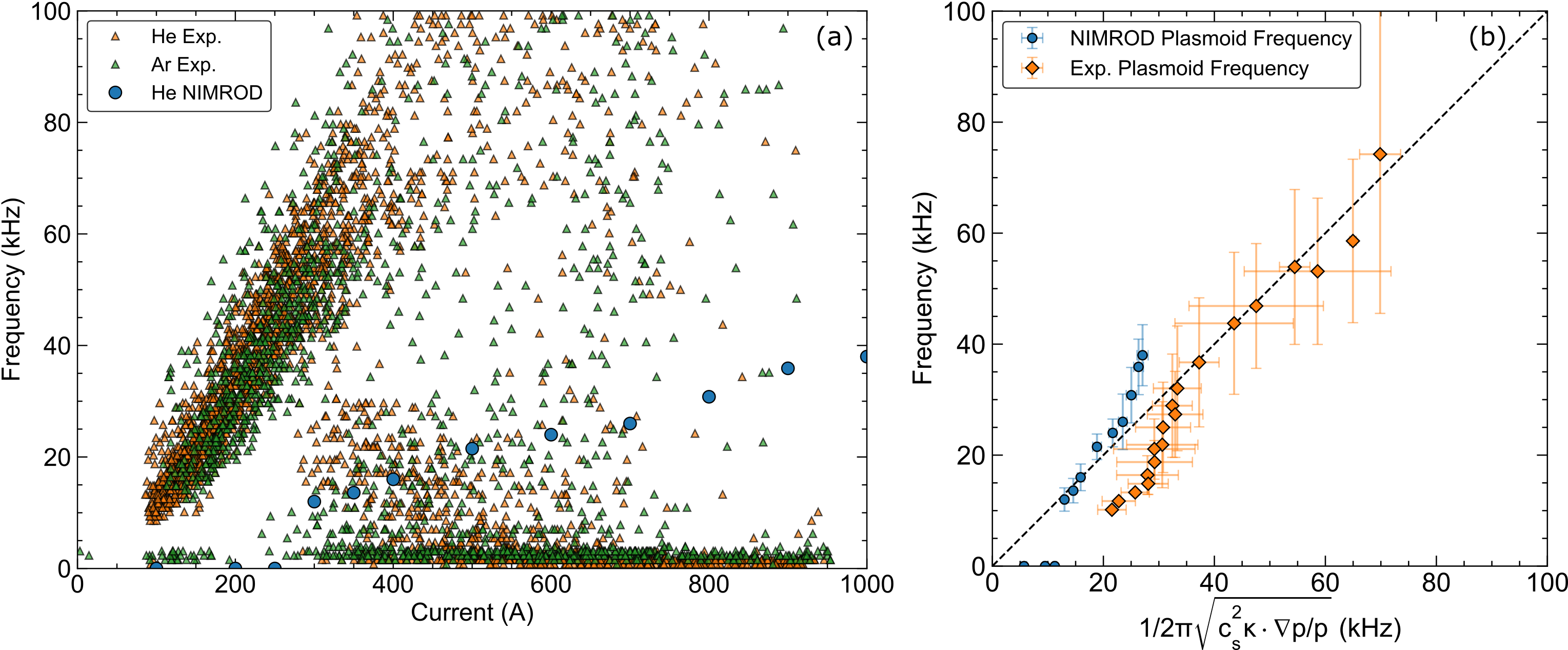
Figure 8: $B_{z}$ fluctuation peak frequencies in the current sheet at $R=30$ cm for Helium and Argon discharges as well as the frequencies of plasmoids present in the NIMROD simulations (a). Plasmoids in both experiment and simulation scale linearly with the injected current and exhibit some stabilizing effect such that no plasmoids exists below roughly 10 kHz in either the experiment or simulations. When the current injection value is translated into a characteristic timescale dependent on the magnetic curvature and pressure gradient at that current value, the plasmoid frequencies in both experiment and simulation are found to scale similarly (b).

Since the plasmoid frequencies scale more strongly with current injection in the experiment than in simulation, the drive mechanism is likely correlated with some quantity other than the current, but likely influenced by it. One possible explanation is that these plasmoids are pressure driven and that the current drive in the experiment produces larger densities in the magnetosphere as a result of ionization, which is not modeled in the simulations. Therefore, calculating a pressure-curvature driven time scale for the loss of equilibrium in experiment and simulations may provide a unifying scaling, as evidenced by Fig. 8(b). Each data point for the experiment in Fig. 8(b) is derived from a 2D flux surface reconstruction and maps of pressure, and temperature averaged over 10 ms windows. Where the flux surface reconstruction is possible (roughly from $t=1.0$ s to $t=1.2$ s), we obtain an estimate of the characteristic frequency $f=\frac{1}{2\pi}\sqrt{c_{s}^{2}{\bf\it\kappa}\cdot\gradient{p}/p}$ calculated near the helmet streamer tip at $R\sim 30$ cm. This results in $\sim 20$ data points whose error in the x-direction is calculated from the error in the magnetic field, temperature, and pressure measurements and whose error in the y-direction represents the full width at half maximum of the peak in the $B_{z}$ power spectral density. The theoretical model and justification for this characteristic time scale are explained in the following section.

5 Heuristic Model of Plasmoid Evolution and Extrapolation to Solar Streamers

A relatively simple heuristic model can be constructed for the plasma expansion in the high-$\beta$ transition region between the hydrostatic equilibrium of the closed flux corona and the hydrodynamic equilibrium of open field lines outside the heliospheric current sheet (HCS). The geometry of such a system is shown in Fig. 9. Writing the momentum equation in terms of the magnetic curvature vector, ${\bf\it\kappa}$, we obtain the dynamic equation for the plasma expansion:

$$\rho\derivative{\mathbf{v_{\perp}}}{t}=-\gradient_{\perp}{p}+\frac{B^{2}}{\mu_{0}}{\bf\it\kappa}-\gradient_{\perp}\frac{B^{2}}{2\mu_{0}}.$$ (1)

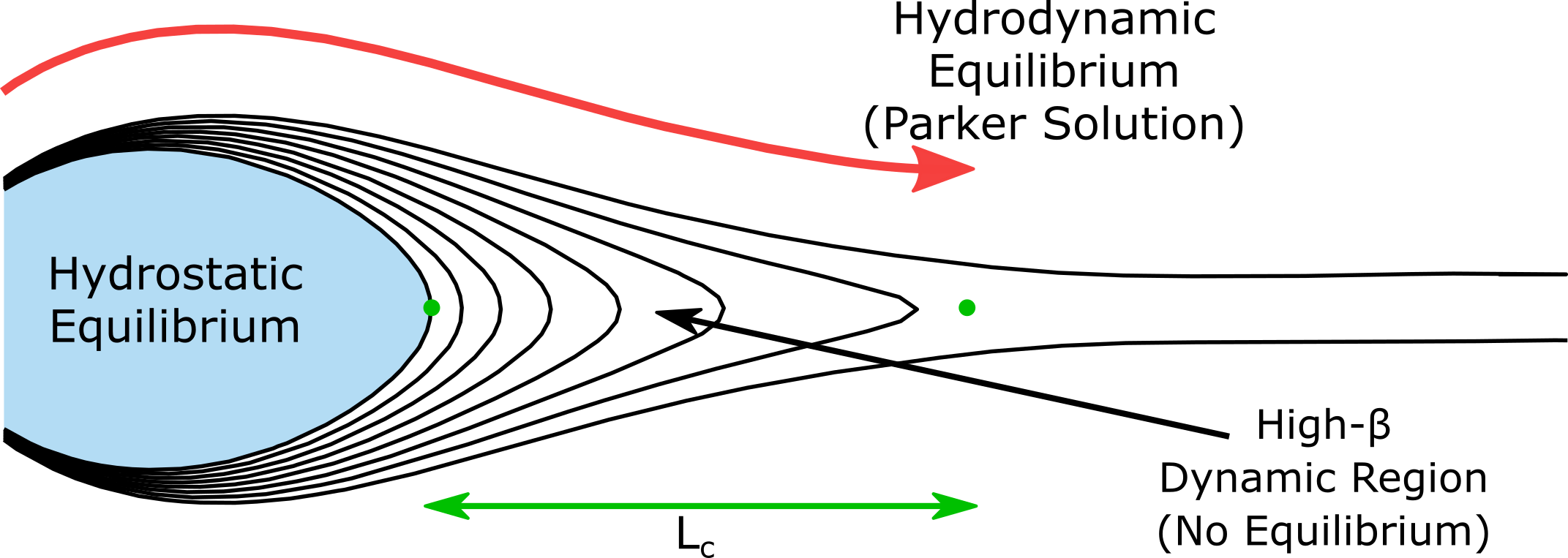
Figure 9: A cartoon drawing of helmet streamer topology with indications of the zones where equilibrium exists; namely, deep in the streamer where there is a hydrostatic solution, and outside the current sheet where Parker’s original hydrodynamic solution is valid. The interface between the two exhibits no equilibrium due to the particle and heat sources present in the corona. This loss of equilibrium is caused by the extremely high values of $\beta$ in this region and result in quasi-periodic plasma blobs which are driven by strong pressure gradients. The length scale $L_{c}$ shown above is the critical length scale of the current sheet that develops from field line stretching before reconnection occurs.

Using the equation of state $p=\rho c_{s}^{2}$, rewriting the right hand side of Eq. 1 in terms of the plasma $\beta=2\mu_{0}p/B^{2}$, and dotting both sides with the curvature vector, ${\bf\it\kappa}$, gives:

$${\bf\it\kappa}\cdot\derivative{\mathbf{v_{\perp}}}{t}=-\frac{c_{s}^{2}}{p}{\bf\it\kappa}\cdot\gradient_{\perp}\left[p\left(1+1/\beta\right)\right]+\frac{2c_{s}^{2}}{\beta}\kappa^{2}.$$ (2)

The left-hand side of this equation can be taken to define a characteristic timescale for the driven loss of equilibrium: ${\bf\it\kappa}\cdot\derivative{\mathbf{v_{\perp}}}{t}\sim-\gamma_{dr}^{2}$. This can be understood as the time required to form a plasmoid of radius $R_{c}=\kappa^{-1}$ due to the acceleration provided by the net force on the right-hand side of Eq. 2. As discussed before, the values of $\beta$ in the current sheet are very large for both the experiment and simulations and range from $10<\beta<50$ throughout the region of interest, denoted as the high-$\beta$ dynamic region in Fig. 9. Therefore, ignoring terms of order $\beta^{-1}$ results in

$$\gamma_{dr}^{2}\sim\frac{c_{s}^{2}}{p}{\bf\it\kappa}\cdot\gradient{p}.$$ (3)

This characteristic time scale can be understood as the time for a sound wave to traverse a distance equivalent to the geometric mean of the pressure gradient scale length and radius of curvature, or equivalently the free-fall time of a plasma parcel under the action of a pressure gradient and adverse magnetic field curvature.

The next step in the derivation of the plasmoid frequency is to show that it is essentially this drive frequency which sets the frequency of reconnection in the current sheet. It will be shown that in this situation the reconnection rate is relatively insensitive to the details of the tearing mode growth rate. We can assume that the current sheet is lengthening at the rate given by the drive timescale $\gamma_{dr}$ because the plasma is frozen to the magnetic field. We can also assume that the lengthening of the current sheet is exponential in time: a result of a transition from quasi-equilibrium to a dynamic system. Incompressibility then requires that the forming sheet is likewise thinning exponentially, such that its thickness $a(t)$ can be described by

$$a(t)=a_{0}e^{-\gamma_{dr}t},$$ (4)

where $a_{0}$ is the thickness at the beginning of the expansion.

As the aspect ratio $L/a$ of this forming current sheet increases, it becomes unstable to a progressively broader spectrum of tearing modes. As argued by Uzdensky & Loureiro (2016), one of those modes — the one whose growth rate, $\gamma_{tear}(t)$, first satisfies $\gamma_{tear}(t_{crit})\sim\gamma_{dr}$ — will eventually grow to become as wide as the forming sheet, thereby disrupting it and leading to plasmoid ejection. This happens at a so-called critical time, $t_{crit}$, whereupon the sheet thickness is

$$a_{crit}\equiv a(t_{crit})=a_{0}e^{-\gamma_{dr}t_{crit}}.$$ (5)

This can be inverted to yield

$$t_{crit}=\gamma_{dr}^{-1}\ln{\left(\frac{a_{0}}{a_{crit}}\right)}.$$ (6)

As we can see, the critical time for reconnection to occur is essentially the same as the drive timescale, $\gamma_{dr}^{-1}$, since the ratio of the initial to the critical current sheet thickness represents only a logarithmic correction. That is, while reconnection is essential to the formation and ejection of plasmoids, the physics of the reconnection onset are such that details of the tearing instability that underlies it (such as the functional form of $\gamma_{tear}(t)$) are not essential to the prediction of the timescale associated with the plasmoid ejection.

Casting the drive timescale for $\gamma_{dr}$ into a characteristic frequency in Hz we obtain

$$f=\frac{1}{2\pi}\sqrt{c_{s}^{2}{\bf\it\kappa}\cdot\gradient{p}/p}.$$ (7)

This time scale is associated with a high-$\beta$ pressure-curvature driven loss of equilibrium. The characteristics of these oscillations — namely that they are electromagnetic, axisymmetric perturbations localized to the region of bad magnetic curvature with a frequency dependent on the pressure gradient — support the notion that these plasmoids are driven by a mechanism similar in nature to flute modes, but likely represent a loss of equilibrium due to particle and heat transport into the streamer rather than a linear instability. It is the frequency in Eq. 7 that empirically provides the unifying scaling between the experimental results and the extended-MHD simulations presented in Fig. 8. Computing this frequency along field lines from the density, temperature and magnetic flux measured by diagnostics in the experiment as well as the simulation shows a local maximum located at the outboard midplane where the curvature is largest. Plotting the measured plasmoid frequencies against this calculated pressure-curvature frequency gives the results in Fig. 8(b) which shows much better agreement between the experiment and simulations and is consistent with the idea that these plasmoids are pressure driven.

If we normalize both the pressure gradient scale length and the magnetic curvature by the critical current sheet length, $L_{c}$, we obtain two dimensionless quantities: $\ell_{b}^{-1}=L_{c}\kappa$ and $\ell_{p}^{-1}=L_{c}\gradient{p}/p$. We can assume, in the laminar plasmoid case, that this critical length, $L_{c}$, is simply the plasmoid length just as reconnection occurs. Substituting these parameters into Eq. 7 provides us with the dimensional scaling below:

$$f=\frac{1}{2\pi}\frac{c_{s}}{L_{c}\sqrt{\ell_{b}\ell_{p}}}.$$ (8)

Given similar normalized length scales, $\ell_{b}$ and $\ell_{p}$, the scaling between experimental and solar wind frequencies is simply the ratio of critical length scales, or plasmoid size, and sound speeds; i.e.:

$$f_{sw}\sim\frac{L_{c,exp}}{L_{c,sw}}\frac{c_{s,sw}}{c_{s,exp}}f_{exp}.$$ (9)

As mentioned before, we will use the plasmoid length as the proxy for $L_{c}$ as it is reasonable to assume for single plasmoids that the associated plasmoid is roughly the size of the current sheet just before it reconnects. For plasmoids in the simulations and experiment, we will take this length scale to be $L_{c,exp}=0.25$ m and in the solar wind we will take this scale to be $L_{c,sw}=1R_{\odot}=7\times 10^{8}$ m which is consistent with observations of plasmoids appearing around $2-4R_{\odot}$ and having a length of $1R_{\odot}$ and width of $0.1R_{\odot}$(Sheeley et al., 2009). Combining these plasmoid length scales with the sound speed typical of the experiment ($c_{s,exp}\sim 13$ km/s) and solar corona ($c_{s,sw}\sim 200$ km/s) gives us a simple scaling relationship between frequencies observed in the lab and in the solar wind as shown in Eq. 10

$$f_{sw}\sim 5.5\times 10^{-9}f_{exp}.$$ (10)

Therefore, the $20-40$ kHz plasmoids observed in both the experiment and simulations correspond to a plasmoid frequency in the solar wind of $110-220~{}\mu$Hz, or periods of $75-150$ minutes — in remarkable agreement with observations (Viall & Vourlidas, 2015).

We note that this model also offers a natural explanation for the existence of laminar and turbulent plasmoid regimes. Increasing the drive (i.e., increasing the injected current in experiments and simulations) leads to a larger $\gamma_{dr}$. When the drive is strong enough such that $\gamma_{dr}\gtrsim v_{A}/L_{c}$, an ejected plasmoid has insufficient time to advect downstream a distance comparable to its length before the subsequent plasmoid is ejected. This leads to plasmoids of different sizes interacting downstream of the reconnection region and more stochastic behavior. For the high drive cases in the simulation, many of the plasmoids are small ($L_{c}\sim 5$ cm), and $v_{A}\sim 2$ km/s, which results in the condition $\gamma_{dr}\gtrsim 40$ kHz which is in good agreement with the onset of the turbulent plasmoids shown in Fig. 5 and Fig. 7(d).

Another mechanism that may be contributing to the turbulent dynamics and to the non-axisymmetric nature of Phase I in the experiment is the transition from single plasmoid formation to multiple simultaneous plasmoid formation. To support this hypothesis, the calculation in Appendix A computes the threshold drive frequency necessary to destabilize shorter wavelength tearing modes in the current sheet. If this threshold is reached we may conclude the subsequent stochastic dynamics are those of a plasmoid chain (Uzdensky et al., 2010; Loureiro et al., 2012) and are responsible for the turbulence in the high-drive cases. Remarkably, as outlined in Appendix A, this threshold frequency is computed to be $f=\gamma_{dr}/(2\pi)\gtrsim 60\,$kHz and is precisely in the range we would expect based on experimental evidence ($\sim 60-100$ kHz).

These two mechanisms allow us to infer a hierarchy of stochasticity associated with the drive strength and therefore the frequency of plasmoid formation. As the drive strength increases, the system experiences a loss of equilibrium and laminar ‘single’ plasmoid ejection. This phase is followed by plasmoids of different ‘generations’ catching up with each other to generate a turbulent medium downstream, but still in the ‘single’ plasmoid regime. This phase applies particularly to the NIMROD simulations which are constrained to be axisymmetric and are below the threshold for multiple plasmoids, yet still exhibit increased turbulence at higher drive. Finally, at the highest drives obtained in the experiment, the threshold to multiple simultaneous plasmoid formation is reached as discussed in Appendix A.

This analysis can be made more quantitative by formally taking into account the geometric effects of the magnetic field and pressure gradient for helmet streamer structures in the solar wind. This process likewise results in blob periodicities in the 1-2 hour range consistent with observations (Viall & Vourlidas, 2015). This model is constructed by taking the streamer-like poloidal field geometry generated during NIMROD simulations and scaling the radius where reconnection occurs to coincide with $3R_{\odot}$ as a characteristic location for PDS formation (Viall & Vourlidas, 2015; Wang et al., 1998; Wang & Hess, 2018). Scaling the magnetic field strength using fits to solar wind data in the ecliptic plane according to Köhnlein (1996), produces a plausible helmet streamer geometry at the proper scale with realistic magnetic field strength. Using fits for plasma temperature and density in the ecliptic (likewise from Köhnlein (1996)) and mapping them to the respective flux surfaces produces a mock helmet streamer with plausible temperature and density profiles.

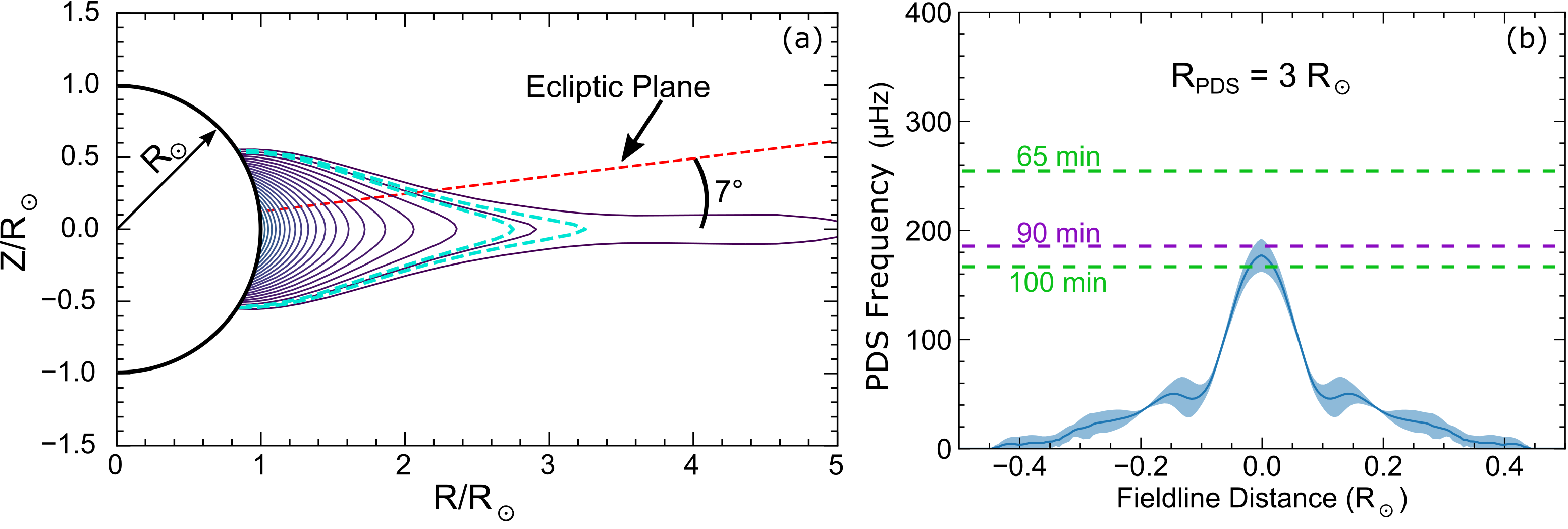
Figure 10: The work of Köhnlein (1996) provides doubly logarithmic fits to Helios data for density, temperature, and magnetic field as a function of heliocentric distance in the ecliptic plane. Mapping these quantities onto the magnetic streamer structure shown in (a) allows us to compute $f=1/2\pi\sqrt{c_{s}^{2}{\bf\it\kappa}\cdot\gradient{p}/p}$ along field lines just inside and just outside the reconnection radius in the same fashion as shown in Fig. 8(b). This results in plasmoid frequencies that are peaked at the streamer cusp as expected and produce periodicities in close agreement with in situ observations for plausible solar wind parameters.

A diagram of this 2D magnetic geometry for this heuristic model is shown in Fig. 10(a). This model enables us to calculate the same characteristic frequency used to unify the scaling between experiment and simulation (Eq. 7) along the field lines in the vicinity of the reconnection site shown as the cyan dashed lines in Fig. 10(a). The result of calculating this frequency along flux surfaces between the cyan dashed flux surfaces in Fig. 10(a) is shown in Fig. 10(b) and plotted as a function of field line distance away from the outboard midplane. In this context, a field line distance of 0 corresponds to the streamer top or the point of highest magnetic curvature where we might expect the highest growth rate of any pressure-curvature driven loss of equilibrium. We can see from this model that the same characteristic timescale used to unify experimental and simulation plasmoid frequencies results in a blob periodicity in the solar wind of $\sim 90$ minutes if formed at $3R_{\odot}$ (Fig. 10b). If the PDS origin radius is increased or decreased, the PDS periodicity likewise increases or decreases respectively in accordance with observations (Wang & Hess, 2018).

6 Conclusions

To accompany the experimental measurements of streamer top reconnection and plasmoid formation in the Parker Spiral current sheet, a wide range of extended-MHD simulations were performed with the NIMROD code. Through measurements and comparisons between experiment and simulation, we showed that this high-$\beta$ loss of equilibrium is related to the pressure gradient and magnetic curvature in the streamer. Specifically, the frequency of expelled plasmoids scales with the pressure gradient and becomes more turbulent as the pressure gradient increases and as one moves further downstream in the current sheet.

A heuristic model for this loss of equilibrium is presented and demonstrates that pressure-curvature driven outflows in the high-$\beta$ transition region of the streamer belt may be responsible for the streamer top reconnection that fuels a portion of the slow solar wind near the HCS. Although the parameters and scale lengths in the experiment are considerably different from those in the solar wind, the pressure driven loss of equilibrium allows both systems to expand outwards at their respective sound speed, advecting the magnetic flux with the ions in the case of the solar wind and with the electrons in the experiment and simulations. While the dynamics of magnetic reconnection are likewise vastly different between the two systems — occurring on sub-ion scales in the experiment and macroscopic (MHD) scales in the solar wind — it is likely that the plasmoid formation rate is governed more by the drive timescale, $\gamma_{dr}$, than by the specifics of magnetic reconnection. As a result, the streamer top may be reconnecting at a rate governed by the particle and heat sourcing on these outer field lines which results in loss of equilibrium rather than a linear instability. This allows for a unified theory to connect observations in drastically different regimes of plasma physics based on empirical evidence. While the underlying reconnection dynamics which set the critical length scale of the current sheet are certainly different, the resulting phenomenon was found to be remarkably similar between experiment and simulation and was also reminiscent of observations of the solar corona performed by the LASCO and SECCHI instrument suites as well as recently by Parker Solar Probe (Lavraud et al., 2020).

The present work was supported by the NASA Earth and Space Sciences - Heliophysics Division Fellowship award no. NNX14AO16H. The BRB facility was constructed with support from the National Science Foundation and is now operated as a Department of Energy National User Facility under DOE fund DE-SC0018266. In addition, this work was supported by the NSF-DOE Partnership in Basic Plasma Science and Engineering award no. PHY-2010136.

Appendix A Reconnection onset in a forming current sheet in the collisional Hall-MHD regime

In Section 5 we alluded to the onset of the tearing mode in the forming current sheet driven by the equilibrium loss. In this Appendix, we present a quantitative, though simplified, derivation aimed at capturing what we think are the key features of this process in our experiments and simulations.

The plasma regime of relevance here can be described by the resistive Hall-MHD framework; namely, we take the ions to be cold, the reconnection dynamics to be happening at sub-ion-skin-depth scales, and the frozen-flux condition to be broken by resistivity. Under these constraints, the expressions for the growth rate of the tearing instability for small and large values of the tearing instability parameter $\Delta^{\prime}$ can be obtained from Attico et al. (2000). They are

$$\gamma\tau_{w}=0.47\,\Delta^{\prime}(\tau_{w}\eta)^{1/2},$$ (11)

in the low $\Delta^{\prime}$ case; and

$$\gamma\tau_{w}=0.69\,(ka)^{3/4}a^{-1/2}(\tau_{w}\eta)^{1/4},$$ (12)

in the large $\Delta^{\prime}$ case. The normalizing timescale that appears in these expressions is sometimes called the whistler time, $\tau_{w}=a^{2}/(d_{i}v_{A})$, with $v_{A}$ the Alfvén speed based on the upstream (reconnecting) magnetic field.

Given a spectrum of unstable wavenumbers, the fastest growing tearing mode is given by the intersection of these two scalings:

$$k_{max}a\approx 1.2\,(\tau_{w}\eta)^{1/7}a^{-2/7},$$ (13)

where we have assumed that the upstream magnetic field is well represented by a $\tanh{x/a}$ profile, whose instability parameter is $\Delta^{\prime}a\approx 2/(ka)$ for $ka\ll 1$. The corresponding growth rate is

$$\gamma_{max}\tau_{w}\approx 0.8(\tau_{w}\eta)^{5/14}a^{-5/7}.$$ (14)

This mode is the fastest-growing mode if the current sheet is long enough that it fits inside the layer; i.e., if $k_{max}L\geq 1$.

From here, the calculation proceeds exactly as prescribed in Uzdensky & Loureiro (2016). We assume, as in Section 5, that the length and the thickness of the forming current sheet expand, or contract, exponentially, with the drive rate $\gamma_{dr}$. Then we find that the $N=1$ mode transitions from the low to the large $\Delta^{\prime}$ regime at the time

$$t_{tr}=\frac{1}{2\gamma_{dr}}\ln\left(\frac{2\pi}{1.2}\frac{a_{0}}{L_{0}}S_{H}^{1/7}\right),$$ (15)

where $S_{H}\equiv d_{i}v_{A}/\eta$ is the Hall Lundquist number, and $a_{0}$ and $L_{0}$ are the initial thickness and length of the current sheet.

On the other hand, one can compute the time $t_{cr}$ at which the growth rate of the $N=1$ mode matches the current sheet formation rate; i.e., solve $\gamma(t)=\gamma_{dr}$ for the $N=1$ mode. This yields

$$t_{cr}\approx\frac{1}{4\gamma_{dr}}\ln\left(\frac{\pi}{0.47}\frac{a_{0}}{L_{0}}\frac{a_{0}^{2}\gamma_{dr}}{d_{i}v_{A}}S_{H}^{1/2}\right).$$ (16)

Finally, one can ask if the $N=1$ mode has the time to transition from the low to the large $\Delta^{\prime}$ regime before reaching its critical time. This occurs when

$$\gamma_{dr}>4.1\frac{a_{0}}{L_{0}}\frac{d_{i}v_{A}}{a_{0}^{2}}S_{H}^{-3/14}.$$ (17)

In other words, if this condition is satisfied, one would expect the forming current sheet to be disrupted by multiple plasmoids (large tearing mode number, $N$); if it is not, then it is the $N=1$ tearing mode that disrupts the forming sheet.

Inserting the values measured or inferred from the experiments into this expression (namely, $a_{0}=0.05\,$m, $L_{0}=0.25\,$m, $d_{i}=0.7\,$m, $c_{s}=13000\,$m s^-1 and $\beta_{e}=20$) yields $f=\gamma_{dr}/(2\pi)\gtrsim 60\,$kHz. This frequency is in remarkable agreement with our experimental results which indicate a transition to the multiple plasmoid regime in the $60-100$ kHz range.

References

- Antiochos et al. (2007) Antiochos, S. K., DeVore, C. R., Karpen, J. T. & Mikić, Z. 2007 Structure and Dynamics of the Sun’s Open Magnetic Field. The Astrophysical Journal 671 (1), 936–946.
- Antiochos et al. (2011) Antiochos, S. K., Mikić, Z., Titov, V. S., Lionello, R. & Linker, J. A. 2011 A MODEL FOR THE SOURCES OF THE SLOW SOLAR WIND. The Astrophysical Journal 731 (2), 112.
- Attico et al. (2000) Attico, N., Califano, F. & Pegoraro, F. 2000 Fast collisionless reconnection in the whistler frequency range. Physics of Plasmas 7 (6), 2381–2387.
- Bale et al. (2019) Bale, S. D., Badman, S. T., Bonnell, J. W., Bowen, T. A., Burgess, D., Case, A. W., Cattell, C. A., Chandran, B. D.G. G., Chaston, C. C., Chen, C. H.K. K., Drake, J. F., de Wit, T. Dudok, Eastwood, J. P., Ergun, R. E., Farrell, W. M., Fong, C., Goetz, K., Goldstein, M., Goodrich, K. A., Harvey, P. R., Horbury, T. S., Howes, G. G., Kasper, J. C., Kellogg, P. J., Klimchuk, J. A., Korreck, K. E., Krasnoselskikh, V. V., Krucker, S., Laker, R., Larson, D. E., MacDowall, R. J., Maksimovic, M., Malaspina, D. M., Martinez-Oliveros, J., McComas, D. J., Meyer-Vernet, N., Moncuquet, M., Mozer, F. S., Phan, T. D., Pulupa, M., Raouafi, N. E., Salem, C., Stansby, D., Stevens, M., Szabo, A., Velli, M., Woolley, T. & Wygant, J. R. 2019 Highly structured slow solar wind emerging from an equatorial coronal hole. Nature 576 (7786), 237–242.
- Bavassano & Bruno (1989a) Bavassano, B. & Bruno, R. 1989a Evidence of local generation of Alfvénic turbulence in the solar wind. Journal of Geophysical Research 94 (A9), 11977.
- Bavassano & Bruno (1989b) Bavassano, B. & Bruno, R. 1989b Large-scale solar wind fluctuations in the inner heliosphere at low solar activity. Journal of Geophysical Research 94 (A1), 168.
- Bavassano et al. (1982) Bavassano, B., Dobrowolny, M., Mariani, F. & Ness, N. F. 1982 Radial evolution of power spectra of interplanetary Alfvénic turbulence. Journal of Geophysical Research 87 (A5), 3617.
- Bavassano et al. (1997) Bavassano, Bruno, Woo, Richard & Bruno, Roberto 1997 Heliospheric plasma sheet and coronal streamers. Geophysical Research Letters 24 (13), 1655–1658.
- Belcher & Davis (1971) Belcher, J. W. & Davis, Leverett 1971 Large-amplitude Alfvén waves in the interplanetary medium, 2. Journal of Geophysical Research 76 (16), 3534–3563.
- Bhat & Loureiro (2018) Bhat, Pallavi & Loureiro, Nuno F. 2018 Plasmoid instability in the semi-collisional regime. Journal of Plasma Physics 84 (6), arXiv: 1804.05145.
- Brueckner et al. (1995) Brueckner, G. E., Howard, R. A., Koomen, M. J., Korendyke, C. M., Michels, D. J., Moses, J. D., Socker, D. G., Dere, K. P., Lamy, P. L., Llebaria, A., Bout, M. V., Schwenn, R., Simnett, G. M., Bedford, D. K. & Eyles, C. J. 1995 The Large Angle Spectroscopic Coronagraph (LASCO). Solar Physics 162 (1-2), 357–402.
- Coleman et al. (1968) Coleman, Paul J., Jr., J., Paul & Jr. 1968 Turbulence, Viscosity, and Dissipation in the Solar-Wind Plasma. The Astrophysical Journal 153, 371.
- Cranmer et al. (2017) Cranmer, Steven R., Gibson, Sarah E. & Riley, Pete 2017 Origins of the Ambient Solar Wind: Implications for Space Weather. Space Science Reviews 212 (3-4), 1345–1384.
- Crooker et al. (2000) Crooker, N. U., Shodhan, S., Gosling, J. T., Simmerer, J., Lepping, R. P., Steinberg, J. T. & Kahler, S. W. 2000 Density extremes in the solar wind. Geophysical Research Letters 27 (23), 3769–3772.
- DeForest et al. (2018) DeForest, C. E., Howard, R. A., Velli, M., Viall, N. & Vourlidas, A. 2018 The Highly Structured Outer Solar Corona. The Astrophysical Journal 862 (1), 18.
- Di Matteo et al. (2019) Di Matteo, S., Viall, N. M., Kepko, L., Wallace, S., Arge, C. N. & MacNeice, P. 2019 Helios Observations of Quasiperiodic Density Structures in the Slow Solar Wind at 0.3, 0.4, and 0.6 AU. Journal of Geophysical Research: Space Physics 124 (2), 837–860.
- Einaudi et al. (1999) Einaudi, Giorgio, Boncinelli, Paolo, Dahlburg, Russell B. & Karpen, Judith T. 1999 Formation of the slow solar wind in a coronal streamer. Journal of Geophysical Research: Space Physics 104 (A1), 521–534.
- Einaudi et al. (2001) Einaudi, Giorgio, Chibbaro, Sergio, Dahlburg, Russell B. & Velli, Marco 2001 Plasmoid Formation and Acceleration in the Solar Streamer Belt. The Astrophysical Journal 547 (2), 1167–1177.
- Endeve et al. (2004) Endeve, Eirik, Holzer, Thomas E. & Leer, Egil 2004 Helmet Streamers Gone Unstable: Two-Fluid Magnetohydrodynamic Models of the Solar Corona. The Astrophysical Journal 603 (1), 307–321.
- Endeve et al. (2003) Endeve, Eirik, Leer, Egil & Holzer, Thomas E. 2003 Two-dimensional Magnetohydrodynamic Models of the Solar Corona: Mass Loss from the Streamer Belt. The Astrophysical Journal 589 (2), 1040–1053.
- Endrizzi et al. (2021) Endrizzi, Douglass, Egedal, J., Clark, M., Flanagan, K., Greess, S., Milhone, J., Millet-Ayala, A., Olson, J., Peterson, E. E., Wallace, J. & Forest, C. B. 2021 Laboratory resolved structure of supercritical perpendicular shocks. Phys. Rev. Lett. 126, 145001.
- Fisk et al. (1998) Fisk, L.A., Schwadron, N.A. & Zurbuchen, T.H. 1998 On the Slow Solar Wind. Space Science Reviews 86 (1/4), 51–60.
- Fisk (2003) Fisk, L. A. 2003 Acceleration of the solar wind as a result of the reconnection of open magnetic flux with coronal loops. Journal of Geophysical Research 108 (A4), 1157.
- Flanagan et al. (2020) Flanagan, K., Milhone, J., Egedal, J., Endrizzi, D., Olson, J., Peterson, E. E., Sassella, R. & Forest, C. B. 2020 Weakly magnetized, hall dominated plasma couette flow. Phys. Rev. Lett. 125, 135001.
- Forest et al. (2015) Forest, C. B., Flanagan, K., Brookhart, M., Clark, M., Cooper, C. M., Désangles, V., Egedal, J., Endrizzi, D., Khalzov, I. V., Li, H., Miesch, M., Milhone, J., Nornberg, M., Olson, J., Peterson, E., Roesler, F., Schekochihin, A., Schmitz, O., Siller, R., Spitkovsky, A., Stemo, A., Wallace, J., Weisberg, D. & Zweibel, E. 2015 The Wisconsin Plasma Astrophysics Laboratory. Journal of Plasma Physics 81 (5), 345810501.
- Fu et al. (2017) Fu, Hui, Madjarska, Maria S., Xia, LiDong, Li, Bo, Huang, ZhengHua & Wangguan, Zhipeng 2017 Charge States and FIP Bias of the Solar Wind from Coronal Holes, Active Regions, and Quiet Sun. The Astrophysical Journal 836 (2), 169.
- Hare et al. (2017) Hare, J. D., Suttle, L., Lebedev, S. V., Loureiro, N. F., Ciardi, A., Burdiak, G. C., Chittenden, J. P., Clayson, T., Garcia, C., Niasse, N., Robinson, T., Smith, R. A., Stuart, N., Suzuki-Vidal, F., Swadling, G. F., Ma, J., Wu, J. & Yang, Q. 2017 Anomalous heating and plasmoid formation in a driven magnetic reconnection experiment. Physical Review Letters 118, 085001.
- Higginson & Lynch (2018) Higginson, A. K. & Lynch, B. J. 2018 Structured Slow Solar Wind Variability: Streamer-blob Flux Ropes and Torsional Alfvén Waves. The Astrophysical Journal 859 (1), 6.
- Kepko & Spence (2003) Kepko, L. & Spence, H. E. 2003 Observations of discrete, global magnetospheric oscillations directly driven by solar wind density variations. Journal of Geophysical Research 108 (A6), 1257.
- Kepko et al. (2002) Kepko, L., Spence, H. E. & Singer, H. J. 2002 ULF waves in the solar wind as direct drivers of magnetospheric pulsations. Geophysical Research Letters 29 (8), 39–1–39–4.
- Kepko et al. (2016) Kepko, L., Viall, N. M., Antiochos, S. K., Lepri, S. T., Kasper, J. C. & Weberg, M. 2016 Implications of L1 observations for slow solar wind formation by solar reconnection. Geophysical Research Letters 43 (9), 4089–4097.
- Köhnlein (1996) Köhnlein, W. 1996 Radial dependence of solar wind parameters in the ecliptic (1.1 - 61AU). Solar Physics 169 (1), 209–213.
- Lapenta & Knoll (2005) Lapenta, Giovanni & Knoll, D. A. 2005 Effect of a Converging Flow at the Streamer Cusp on the Genesis of the Slow Solar Wind. The Astrophysical Journal 624 (2), 1049–1056.
- Lavraud et al. (2020) Lavraud, B., Fargette, N., Réville, V., Szabo, A., Huang, J., Rouillard, A. P., Viall, N., Phan, T. D., Kasper, J. C., Bale, S. D., Berthomier, M., Bonnell, J. W., Case, A. W., de Wit, T. Dudok, Eastwood, J. P., Génot, V., Goetz, K., Griton, L. S., Halekas, J. S, Harvey, P., Kieokaew, R., Klein, K. G., Korreck, K. E., Kouloumvakos, A., Larson, D. E., Lavarra, M., Livi, R., Louarn, P., MacDowall, R. J., Maksimovic, M., Malaspina, D., Nieves-Chinchilla, T., Pinto, R. F., Poirier, N., Pulupa, M., Raouafi, N. E., Stevens, M. L., Toledo-Redondo, S. & Whittlesey, P. L. 2020 The heliospheric current sheet and plasma sheet during parker solar probe’s first orbit. The Astrophysical Journal 894 (2), L19.
- Loureiro et al. (2012) Loureiro, N. F., Samtaney, R., Schekochihin, A. A. & Uzdensky, D. A. 2012 Magnetic reconnection and stochastic plasmoid chains in high-Lundquist-number plasmas. Physics of Plasmas 19 (4), 042303–042303, arXiv: 1108.4040.
- Luttrell & Richter (1987) Luttrell, A. H. & Richter, A. K. 1987 The Role of Alfvenic Fluctuations in MHD Turbulence Evolution between 0.3 and 1.0 AU. Sixth International Solar Wind Conference, Proceedings of the conference held 23-28 August, 1987 at YMCA of the Rockies, Estes Park, Colorado. Edited by V.J. Pizzo, T. Holzer, and D.G. Sime. NCAR Technical Note NCAR/TN-306+Proc, Volume 2, 1987., p.335 p. 335.
- Marsch & Tu (1990a) Marsch, E. & Tu, C.-Y. 1990a On the radial evolution of MHD turbulence in the inner heliosphere. Journal of Geophysical Research 95 (A6), 8211.
- Marsch & Tu (1990b) Marsch, E. & Tu, C.-Y. 1990b Spectral and spatial evolution of compressible turbulence in the inner solar wind. Journal of Geophysical Research 95 (A8), 11945.
- Neugebauer et al. (2016) Neugebauer, Marcia, Reisenfeld, Daniel & Richardson, Ian G. 2016 Comparison of algorithms for determination of solar wind regimes. Journal of Geophysical Research: Space Physics 121 (9), 8215–8227.
- Neugebauer & Snyder (1962) Neugebauer, Marcia & Snyder, Conway W 1962 Solar Plasma Experiment. Science 138 (3545), 1095–1097.
- Olson et al. (2016) Olson, J., Egedal, J., Greess, S., Myers, R., Clark, M., Endrizzi, D., Flanagan, K., Milhone, J., Peterson, E., Wallace, J., Weisberg, D. & Forest, C.B. 2016 Experimental Demonstration of the Collisionless Plasmoid Instability below the Ion Kinetic Scale during Magnetic Reconnection. Physical Review Letters 116 (25), 1–5.
- Parker (1958) Parker, Eugene N. 1958 Dynamics of the Interplanetary Gas and Magnetic Fields. The Astrophysical Journal 128, 664–676.
- Peterson et al. (2019) Peterson, Ethan E., Endrizzi, Douglass A., Beidler, Matthew, Bunkers, Kyle J., Clark, Michael, Egedal, Jan, Flanagan, Ken, McCollam, Karsten J., Milhone, Jason, Olson, Joseph, Sovinec, Carl R., Waleffe, Roger, Wallace, John & Forest, Cary B. 2019 A laboratory model for the Parker spiral and magnetized stellar winds. Nature Physics p. 1.
- Rouillard et al. (2011) Rouillard, A. P., Sheeley, N. R., Cooper, T. J., Davies, J. A., Lavraud, B., Kilpua, E. K. J., Skoug, R. M., Steinberg, J. T., Szabo, A., Opitz, A. & Sauvaud, J.-A. 2011 THE SOLAR ORIGIN OF SMALL INTERPLANETARY TRANSIENTS. The Astrophysical Journal 734 (1), 7.
- Sanchez-Diaz et al. (2019) Sanchez-Diaz, E., Rouillard, A. P., Lavraud, B., Kilpua, E. & Davies, J. A. 2019 In Situ Measurements of the Variable Slow Solar Wind near Sector Boundaries. The Astrophysical Journal 882 (1), 51, arXiv: 1911.09683.
- Sheeley et al. (2009) Sheeley, N. R., Lee, D. D.-H., Casto, K. P., Wang, Y.-M. & Rich, N. B. 2009 THE STRUCTURE OF STREAMER BLOBS. The Astrophysical Journal 694 (2), 1471–1480.
- Sheeley, Jr. et al. (1997) Sheeley, Jr., N. R., Wang, Y.-M., Hawley, S. H., Brueckner, G. E., Dere, K. P., Howard, R. A., Koomen, M. J., Korendyke, C. M., Michels, D. J., Paswaters, S. E., Socker, D. G., St. Cyr, O. C., Wang, D., Lamy, P. L., Llebaria, A., Schwenn, R., Simnett, G. M., Plunkett, S. & Biesecker, D. A. 1997 Measurements of Flow Speeds in the Corona Between 2 and 30 . The Astrophysical Journal 484 (1), 472–478.
- Sovinec et al. (2004) Sovinec, C.R., Glasser, A.H., Gianakon, T.A., Barnes, D.C., Nebel, R.A., Kruger, S.E., Schnack, D.D., Plimpton, S.J., Tarditi, A. & Chu, M.S. 2004 Nonlinear magnetohydrodynamics simulation using high-order finite elements. Journal of Computational Physics 195 (1), 355–386.
- Sovinec & King (2010) Sovinec, C.R. & King, J.R. 2010 Analysis of a mixed semi-implicit/implicit algorithm for low-frequency two-fluid plasma modeling. Journal of Computational Physics 229 (16), 5803–5819.
- Stephenson & Walker (2002) Stephenson, J. A. E. & Walker, A. D. M. 2002 HF radar observations of Pc5 ULF pulsations driven by the solar wind. Geophysical Research Letters 29 (9), 8–1–8–4.
- Uzdensky & Loureiro (2016) Uzdensky, D. A. & Loureiro, N. F. 2016 Magnetic Reconnection Onset via Disruption of a Forming Current Sheet by the Tearing Instability. Physical Review Letters 116 (10), arXiv: 1411.4295.
- Uzdensky et al. (2010) Uzdensky, D. A., Loureiro, N. F. & Schekochihin, A. A. 2010 Fast magnetic reconnection in the plasmoid-dominated regime. Physical Review Letters 105, 235002.
- Viall et al. (2008) Viall, N. M., Kepko, L. & Spence, H. E. 2008 Inherent length-scales of periodic solar wind number density structures. Journal of Geophysical Research: Space Physics 113 (A7), n/a–n/a.
- Viall & Vourlidas (2015) Viall, Nicholeen M. & Vourlidas, Angelos 2015 PERIODIC DENSITY STRUCTURES AND THE ORIGIN OF THE SLOW SOLAR WIND. The Astrophysical Journal 807 (2), 176.
- Wang et al. (1997) Wang, Y.-M., Sheeley, Jr., N. R., Howard, R. A., Kraemer, J. R., Rich, N. B., Andrews, M. D., Brueckner, G. E., Dere, K. P., Koomen, M. J., Korendyke, C. M., Michels, D. J., Moses, J. D., Paswaters, S. E., Socker, D. G., Wang, D., Lamy, P. L., Llebaria, A., Vibert, D., Schwenn, R. & Simnett, G. M. 1997 Origin and Evolution of Coronal Streamer Structure During the 1996 Minimum Activity Phase. The Astrophysical Journal 485 (2), 875–889.
- Wang & Hess (2018) Wang, Y.-M. & Hess, P. 2018 Gradual Streamer Expansions and the Relationship between Blobs and Inflows. The Astrophysical Journal 859 (2), 135.
- Wang et al. (1998) Wang, Y.-M., Sheeley, Jr., N. R., Walters, J. H., Brueckner, G. E., Howard, R. A., Michels, D. J., Lamy, P. L., Schwenn, R. & Simnett, G. M. 1998 Origin of Streamer Material in the Outer Corona. The Astrophysical Journal 498 (2), L165–L168.
- Wu et al. (2000) Wu, S. T., Wang, A. H., Plunkett, S. P. & Michels, D. J. 2000 Evolution of Global-Scale Coronal Magnetic Field due to Magnetic Reconnection: The Formation of the Observed Blob Motion in the Coronal Streamer Belt. The Astrophysical Journal 545 (2), 1101–1115.