Vibrational Effects on the Formation of Quantum $W$ States

Abstract

We theoretically investigate the formation of $W$ states in a tripartite system composed of three charge qubits coupled to vibrational modes. The electromechanical coupling is responsable for second order virtual processes that result in an effective electron-electron interaction between neighbor qubits, which yields to the formation of $W$ states. Based on the Lang-Firsov transformation and perturbation theory, we analytically solve the quantum dynamics, providing a mathematical expression for the maximally entangled $W$ state. Dephasing is also taken into accout, paying particular attention on the robustness of bipartite entanglement against local dephasing processes.

I Introduction

Entanglement is one of the main features of quantum mechanics that make quantum computers so advantageous compared to classical computers.barnett2009 Entangled states appeared early in the quantum mechanics development in the context of the Einstein, Podolsky and Rosen (EPR) paradoxy.einstein1935 Since then quantum entanglement became a prominent resource for quantum communication and quantum information processing,chuang2004 with potential applications in problems such as prime factoringlucero2012 and quantum simulations.qiu2020

In the context of solid-state system, superconducting-based quantum devices have received great attention in the last decade, as they constitute one of the leading system for implementation of quantum computation.devoret2013 For instance, transmon qubits in superconducting chips have been used to generate the Greenberg-Horner-Zeilinger state.barends2014 The GHZ stategreenberger2007 was also found in a three-qubit superconducting circuit,dicarlo2010 and both GHZ and Wdur2000 states were reported in superconducting phase qubits.neeley2010 Superconducting qubits have also been applied for quantum network.yin2015 Additionally, a recent experiment with 53-qubits is an outstading example of the recent progress of the superconducting-based quantum computation.arute2019

Even though superconducting qubits have received a great deal of attention and significant progresses have been achieved, there are many other potential solid-state devices that can be applied to manipulate qubits. For instance, it was demonstrated coherent oscillations of single electron spin in GaAs quantum dots,koppens2005 and coherent control of coupled electron spins was reported.petta2005 Additionally, it was demonstrated initialization, control and readout of three-electron spin qubits.medford2013 More recently, silicon-based systems have being receved a growing attention as it was found long electron spin coherence times.tyryshkin2012 ; maune2012 ; veldhorst2014 ; kawakami2014 For instance, in the context of silicon based system it was recently reported the implementation of CNOT gates and single-qubit operations.veldhorst2015 It was also demonstrated an efficient resonantly driven CNOT gate for electron spins in silicon double quantum dot structure.zajac2018 In addition, SWAP two-qubit exchange gate between phosphorus donor electron spin qubits in silicon was recently reported.he2019 Also, semiconductor quantum dot system have been proposed as solid state devices to construct GHZ state.nogueira2020 Recently, it was shown that highly entangled two-qubit states can be achieved due to electron-vibrational mode coupling in molecular systems.souza2019 Here we extend this previous work by showing that electromechanical coupling can also be a useful tool to generate entangled three-qubit $W$ states in electronic solid-state devices.

The $W$ states consist of a special class of entangled state, being of the formdur2000

$$\mathinner{|{W}\rangle}=a\mathinner{|{001}\rangle}+b\mathinner{|{010}\rangle}+c\mathinner{|{100}\rangle},\phantom{x}$$ (1)

($|a|^{2}+|b|^{2}+|c|^{2}=1$) which when one of the qubits is traced out leaves a partially entangled pair of qubits. This is an example of a two-way entangled state,wong2001 that is robust against losses in one of the qubits.dur2000 Being of great importance for quantum information processing, such as two-party quantum teleportation,jung2008 and superdense coding, the $W$ state have been both theoretically and experimentally investigated in an array of superconducting microwave resonator,gangat2013 in spin systems,li2015 ; chen2017 in superconducting quantum interference device.kang2016 Recently, three-photon $W$ states were demonstrated in optical fibers.fang2019

In the present work we investigated a tripartite system composed of three charge qubits that interact with vibrational degrees of freedom of a nearby molecular structure, that can be, for instance, carbon nanotubes as pointed out in Ref. [souza2019, ]. Based on this previous work, here we derive a model Hamiltonian based on the Lang-Firsov transformation, that explicitly shows a charge-charge attractive like interaction (a typical superconductivity related phenomena), that is behind the formation of the $W$ state being generated. Based on perturbation theory a simple three dimensional model can be derived, expressed in the reduced computational base $\{\mathinner{|{001}\rangle},\mathinner{|{010}\rangle},\mathinner{|{100}\rangle}\}$, that recovers the main physical ingredients behind our full numerical results. Our paper is organized as follows, in Sec. II we present our theoretical model and analytical results, in Sec. III we show the quantum dynamics of our system, paying particular attention to the formation of the $\mathinner{|{W}\rangle}$ state. In Sec. IV we account for dephasing processes and finally in Sec. V we summarize our conclusions.

Figure 1: Illustration of the considered system. Three charge qubits couple to two bosonic environments. No direct coupling between the qubits are considered, so the qubits indirectly couple to each other via vibrational modes of the bosonic subsystems. As a result, the electrons in the qubits experience an attractive interaction, that gives rise to the formation of highly entangled $\mathinner{|{W}\rangle}$ state.

II Theoretical Model

Consider a multipartite system composed of five subspaces, $\mathcal{H}=\mathcal{H}_{qb1}\otimes\mathcal{H}_{qb2}\otimes\mathcal{H}_{qb3}\otimes\mathcal{H}_{v}\otimes\mathcal{H}_{v}$, where the first three subspaces correspond to the qubits A, B and C, while the last two subspaces are associated to the vibrational modes, as illustrated in Fig. (1). The qubits Hamiltonian is given by

$$H_{\mathrm{qubits}}=\bigoplus_{n=1}^{3}[\frac{\delta_{n}}{2}\sigma_{z}^{(n)}+t_{n}\sigma_{x}^{(n)}],$$ (2)

where the Kronecker sum means $\bigoplus_{1}^{3}a_{n}A^{(n)}=a_{1}A\otimes I\otimes I+a_{2}I\otimes A\otimes I+a_{3}I\otimes I\otimes A$. Also, $\delta_{n}$ and $t_{n}$ are the detuning between the electronic levels and the intra qubit charge tunneling, respectively. The vibrational modes degree of freedom are described according to

$$H_{\mathrm{v}}=\omega_{1}B^{\dagger}B\otimes I_{v}+\omega_{2}I_{v}\otimes B^{\dagger}B,$$ (3)

where $\omega_{i}$ is the energy of the $i$-th vibrational mode. The operator $B$ ($B^{\dagger}$) annihilates (creates) vibrational excitations, and $I_{v}$ is the identity matrix in the vibrational subspace. The electromechanical coupling is given in terms of projection operators as

$$V = \bigoplus_{n=1}^{3}[g_{n}P_{0}^{(n)}]\otimes[(B^{\dagger}+B)\otimes I_{v}]+$$ (4)

$$\bigoplus_{n=1}^{3}[g_{n}P_{1}^{(n)}]\otimes[I_{v}\otimes(B^{\dagger}+B)],$$

where $P_{i}=\mathinner{|{i}\rangle}\mathinner{\langle{i}|}$ and $g_{n}$ is the coupling parameter between the electronic and vibrational degrees of freedom. This means that state $\mathinner{|{0}\rangle}$ couples to the vibrational mode characterized by $\omega_{1}$, while state $\mathinner{|{1}\rangle}$ couples to the vibrational model with $\omega_{2}$. footnote1 This feature is illustrated in Fig. (1). As recently shown in Ref. [souza2019, ], to deal with this particular model (which considers the electron-vibrational mode coupling) it is more convenient to use the Lang-Firsov canonical transformation.mahan2000 Defining the operator

$$S = \bigoplus_{n=1}^{3}[\lambda_{n}P_{0}^{(n)}]\otimes[(B^{\dagger}-B)\otimes I_{v}]+$$ (5)

$$\bigoplus_{n=1}^{3}[\lambda_{n}P_{1}^{(n)}]\otimes[I_{v}\otimes(B^{\dagger}-B)],$$

where $\lambda_{n}=g_{n}/\omega_{n}$, we can perform the transformation $\bar{H}=e^{S}He^{-S}$. After a straightforward calculation we find the following set of equations,

$$\bar{H}_{\mathrm{qubits}} = \bigoplus_{n=1}^{3}\frac{\delta_{n}}{2}\sigma_{z}^{(n)}-\frac{1}{\omega}(g_{1}^{2}+g_{2}^{2}+g_{3}^{2})$$

$$- \frac{g_{1}g_{2}}{\omega}(\sigma_{z}\otimes\sigma_{z}\otimes I+I^{\otimes 3})$$

$$- \frac{g_{1}g_{3}}{\omega}(\sigma_{z}\otimes I\otimes\sigma_{z}+I^{\otimes 3})$$

$$- \frac{g_{2}g_{3}}{\omega}(I\otimes\sigma_{z}\otimes\sigma_{z}+I^{\otimes 3}).$$

Notice that the last three terms of Eq.(II) can be associated to an attractive Coulomb like interaction. The vibrational modes remains as $\bar{H}_{\mathrm{v}}=\omega_{1}B^{\dagger}B\otimes I_{v}+\omega_{2}I_{v}\otimes B^{\dagger}B$. Finally, the interaction term takes the form

$$\bar{V} = t_{1}(\sigma_{+}\otimes I\otimes I\otimes D(\lambda_{1})\otimes D(-\lambda_{1})+h.c.)+$$ (7)

$$t_{2}(I\otimes\sigma_{+}\otimes I\otimes D(\lambda_{2})\otimes D(-\lambda_{2})+h.c.)+$$

$$t_{3}(I\otimes I\otimes\sigma_{+}\otimes D(\lambda_{3})\otimes D(-\lambda_{3})+h.c.),$$

where $\sigma_{+}=|0\rangle\langle 1|$, $\sigma_{-}=|1\rangle\langle 0|$ and $D(\pm\lambda_{i})=e^{\pm\lambda_{i}(B^{\dagger}-B)}$ is the displacement operator.scully1997 In what follows we assume $t_{i}=t$, $\omega_{i}=\omega$ and $g_{i}=g$, so that $\lambda_{i}=\lambda=g/\omega$.

From the transformed model, we can easily find the system eigenenergies in the absence of tunneling, i.e., $\bar{V}=0$. In what follows, this coupling term will be considered as a perturbation. The eigenenergies of $\bar{H}_{0}=\bar{H}_{\mathrm{}}+\bar{H}_{\mathrm{v}}$ can be divided in four energy groups. The higher and lower energetic ones,

$$\varepsilon_{000,ml}=\frac{1}{2}(\delta_{1}+\delta_{2}+\delta_{3})-\frac{3g^{2}}{\omega}+(m+l)\omega,$$ (8)

and

$$\varepsilon_{111,ml}=-\frac{1}{2}(\delta_{1}+\delta_{2}+\delta_{3})-\frac{3g^{2}}{\omega}+(m+l)\omega,$$ (9)

respectively. The upper intermediate ones,

$$\varepsilon_{001,ml} = \frac{1}{2}(+\delta_{1}+\delta_{2}-\delta_{3})+\frac{g^{2}}{\omega}+(m+l)\omega,$$ (10)

$$\varepsilon_{010,ml} = \frac{1}{2}(+\delta_{1}-\delta_{2}+\delta_{3})+\frac{g^{2}}{\omega}+(m+l)\omega,$$ (11)

$$\varepsilon_{100,ml} = \frac{1}{2}(-\delta_{1}+\delta_{2}+\delta_{3})+\frac{g^{2}}{\omega}+(m+l)\omega,$$ (12)

and the lower intermediate ones,

$$\varepsilon_{011,ml} = \frac{1}{2}(+\delta_{1}-\delta_{2}-\delta_{3})+\frac{g^{2}}{\omega}+(m+l)\omega,$$ (13)

$$\varepsilon_{101,ml} = \frac{1}{2}(-\delta_{1}+\delta_{2}-\delta_{3})+\frac{g^{2}}{\omega}+(m+l)\omega,$$ (14)

$$\varepsilon_{110,ml} = \frac{1}{2}(-\delta_{1}-\delta_{2}+\delta_{3})+\frac{g^{2}}{\omega}+(m+l)\omega.$$ (15)

A constant energy shift of $-6g^{2}/\omega$ was omitted in all the energies above. If we set the detunings at $\delta_{1}=\delta_{2}=\delta_{3}=\delta$ we find $\varepsilon_{000,ml}=\frac{3}{2}\delta-\frac{3g^{2}}{\omega}+(m+l)\omega$, $\varepsilon_{111,ml}=-\frac{3}{2}\delta-\frac{3g^{2}}{\omega}+(m+l)\omega$, and the degenerate levels $\varepsilon_{001,ml}=\varepsilon_{010,ml}=\varepsilon_{100,ml}=\frac{1}{2}\delta+\frac{g^{2}}{\omega}+(m+l)\omega$, and $\varepsilon_{011,ml}=\varepsilon_{101,ml}=\varepsilon_{110,ml}=-\frac{1}{2}\delta+\frac{g^{2}}{\omega}+(m+l)\omega$. In order to have a graphical view of these energy levels we calculate the spectral function of the system. Consider the retarded Green function,jauho2008

$$G_{nn^{\prime}}^{r}(t-t^{\prime})=-i\theta(t-t^{\prime})\mathinner{\langle{\phi_{n}}|}e^{-i\bar{H}_{0}(t-t^{\prime})}\mathinner{|{\phi_{n^{\prime}}}\rangle}.$$ (16)

Assuming $\mathinner{|{\phi_{n}}\rangle}$ as the eigenstate of $\bar{H}_{0}$, $\bar{H}_{0}\mathinner{|{\phi_{n}}\rangle}=\varepsilon_{n}\mathinner{|{\phi_{n}}\rangle}$, we can write

$$G_{nn^{\prime}}^{r}(t-t^{\prime})=-i\theta(t-t^{\prime})\delta_{nn^{\prime}}e^{-i\varepsilon_{n}(t-t^{\prime})}.$$ (17)

Fourier transforming $G_{nn^{\prime}}^{r}(t-t^{\prime})$ we find

$$G_{nn^{\prime}}^{r}(\epsilon)=\frac{\delta_{nn^{\prime}}}{\epsilon-\varepsilon_{n}+i\eta},$$ (18)

where $\eta\to 0^{+}$. The spectral function, defined as $A_{n}(\epsilon)=-2\mathrm{Im}[G_{nn}^{r}(\epsilon)]$, is then given by

$$A_{n}(\epsilon)=\frac{2\eta}{(\epsilon-\varepsilon_{n})^{2}+\eta^{2}}.$$ (19)

In Fig. (2) we show the total spectral function $A(\epsilon)=\sum_{n}A_{n}(\epsilon)$ as function of $\epsilon$ and $\delta$ for $t_{n}=0$. We observe two spaced groups of four branches each. The high energetic ones are basically replicas of the lowest ones, corresponding to vibrational modes $n=1$ and $m=0$ or $n=0$ and $m=1$. Focusing on the low energetic levels ($n=0$, $m=0$) we have $\varepsilon_{000,ml}=\frac{3}{2}\delta-\frac{3g^{2}}{\omega}$ and $\varepsilon_{111,ml}=-\frac{3}{2}\delta-\frac{3g^{2}}{\omega}$, with high slope $3/2$ (in modulus) as $\delta$ increases. The other two branches are given by $\varepsilon_{001,00}=\varepsilon_{010,00}=\varepsilon_{100,00}=\frac{1}{2}\delta+\frac{g^{2}}{\omega}$ and $\varepsilon_{011,00}=\varepsilon_{101,00}=\varepsilon_{110,00}=-\frac{1}{2}\delta+\frac{g^{2}}{\omega}$. If $\delta$ is properly tunned such that the levels $\varepsilon_{001,00}$, $\varepsilon_{010,00}$ and $\varepsilon_{100,00}$ are relatively far from the other branches, the system becomes suitable for the generation of $\mathinner{|{W}\rangle}$ states within subspace $\mathcal{E}_{\mathrm{w}}=\mathrm{span}\{\mathinner{|{100}\rangle},\mathinner{|{010}\rangle},\mathinner{|{001}\rangle}\}$. It is important to emphasize that to form $W$ states within this electronic subpsace, the physical parameters should be set along the branches corresponding to the energies $\varepsilon_{001,00}=\varepsilon_{010,00}=\varepsilon_{100,00}$. Without loss of generality, we set our parameters to the values as indicated by the green dot in Fig. (2). Other points could also be chosen, as long as they satisfy the condition of being far apart from other branches. With this assumption, it is convenient to divide the system into two subspaces, the relevant one, given by the projector operator $P=(\mathinner{|{100}\rangle}\mathinner{\langle{100}|}+\mathinner{|{010}\rangle}\mathinner{\langle{010}|}+\mathinner{|{001}\rangle}\mathinner{\langle{001}|})\otimes\mathinner{|{00}\rangle}\mathinner{\langle{00}|}$, and the irrelevant one $Q=I-P$, composed by all the other states in the computational basis. In order to estimate the effective coupling between the states in $P$ subspace, we apply the second order perturbation theory. For instance, we can calculate the coupling between states $\mathinner{|{100}\rangle}$ and $\mathinner{|{010}\rangle}$,

$$\Omega_{100,010} = -\sum_{i,j,k}\frac{\mathinner{\langle{100}|}\bar{V}\mathinner{|{ijk}\rangle}\mathinner{\langle{ijk}|}\bar{V}\mathinner{|{010}\rangle}}{\varepsilon_{ijk,00}-\varepsilon_{100,00}},$$ (20)

where we consider only $n=m=0$ for the vibrational states, as high energetic levels contributions to the sum are neglected. More specifically we have,

$$\Omega_{100,010} = -\frac{\mathinner{\langle{100}|}\bar{V}\mathinner{|{000}\rangle}\mathinner{\langle{000}|}\bar{V}\mathinner{|{010}\rangle}}{\varepsilon_{000,00}-\varepsilon_{100,00}}$$ (21)

$$-\frac{\mathinner{\langle{100}|}\bar{V}\mathinner{|{110}\rangle}\mathinner{\langle{110}|}\bar{V}\mathinner{|{010}\rangle}}{\varepsilon_{110,00}-\varepsilon_{100,00}},$$

which results in,

$$\Omega_{100,010}=-\frac{4g^{2}t^{2}e^{-2\lambda^{2}}}{\omega\delta(\delta-\frac{4g^{2}}{\omega})},$$ (22)

where the identity $\mathinner{\langle{m}|}D(\lambda)\mathinner{|{0}\rangle}=\lambda^{m}e^{-\lambda^{2}/2}/\sqrt{m!}$ was applied.scully1997 Similar results hold for $\Omega_{100,001}$ and $\Omega_{010,001}$. Therefore, we can write an effective model in the subspace $P$ as $H_{eff}=\Omega h$, where

$$h=\mathinner{|{100}\rangle}\mathinner{\langle{010}|}+\mathinner{|{100}\rangle}\mathinner{\langle{001}|}+\mathinner{|{010}\rangle}\mathinner{\langle{001}|}+H.c.$$ (23)

The eigenvalues of $h$ are given by $a^{\prime}=2$, $b^{\prime}=c^{\prime}=-1$, with corresponding eigenvectors

$$\mathinner{|{\bar{0}^{\prime}}\rangle} = \frac{1}{\sqrt{3}}(\mathinner{|{\bar{0}}\rangle}+\mathinner{|{\bar{1}}\rangle}+\mathinner{|{\bar{2}}\rangle})$$ (24)

$$\mathinner{|{\bar{1}^{\prime}}\rangle} = \frac{1}{\sqrt{6}}(\mathinner{|{\bar{0}}\rangle}+\mathinner{|{\bar{1}}\rangle}-2\mathinner{|{\bar{2}}\rangle})$$ (25)

$$\mathinner{|{\bar{2}^{\prime}}\rangle} = \frac{1}{\sqrt{2}}(\mathinner{|{\bar{0}}\rangle}-\mathinner{|{\bar{1}}\rangle}).$$ (26)

From here on, we take the shorthand notation $\mathinner{|{\bar{0}}\rangle}=\mathinner{|{100}\rangle}$, $\mathinner{|{\bar{1}}\rangle}=\mathinner{|{010}\rangle}$ and $\mathinner{|{\bar{2}}\rangle}=\mathinner{|{001}\rangle}$. With this simple model we can proceed to the dynamics analysis.

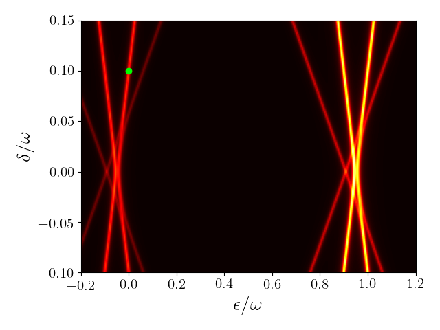
Figure 2: Spectral function of the system as function of energy $\epsilon$ and detunning $\delta$. For small values of energy we have a set of four branches, corresponding to Eqs. (8)-(15) with $m=l=0$. The two low intensity branches are given by $\varepsilon_{000,00}=(3/2)\delta$ and $\varepsilon_{111,00}=-(3/2)\delta$, while the other two high intensity branches are due to the degenerate energies $\varepsilon_{001,00}=\varepsilon_{010,00}=\varepsilon_{100,00}=(1/2)\delta$ and $\varepsilon_{011,00}=\varepsilon_{101,00}=\varepsilon_{110,00}=-(1/2)\delta$. For high values of energy we find replicas of these branches as the energy of the vibrational modes increases with $(n+l)\omega$. To form a $\mathinner{|{W}\rangle}$ state within subspace $\mathcal{E}_{\mathrm{w}}$ spanned by $\{\mathinner{|{001}\rangle},\mathinner{|{010}\rangle},\mathinner{|{100}\rangle}\}$ we need to set the energy parameters in such a way that the corresponding energies $\varepsilon_{001,00}$, $\varepsilon_{010,00}$ and $\varepsilon_{100,00}$ are well isolated from the other energy levels. The green dot in the figure indicates the set of energies configuration used in our simulation to obtain a $\mathinner{|{W}\rangle}$ state within the aforementioned subspace. Virtual processes take place between the many branches shown in order to construct this state.

Physical Parameters. In the experimental point of view, our model can describe carbon nanotube (CNT) quantum dots, as recently proposed in Ref. [souza2019, ] for two qubits entanglement. In the context of CNT the vibrational mode frequency will be assumed around $\omega=20$ meV, in agreement with typical values found in CNT.leroy2004 The intra qubit electron hopping will be considered $t=0.1$ meV, in accordance with the coupling parameter found in experimental setup on parallel CNT quantum dots.gob2013 Also, the electron-phonon coupling parameter $g$ can be experimentally adjusted in CNT,benyamini2014 here in particular we set $g=0.1\omega$. Different $g$ values were explored in the context of quantum transport in CNT quantum dots.walter2013 ; sowa2017 Even though we assume experimentally feasible parameters in the context CNT quantum dots, the theoretical results presented below can in principle be found in different system, as soon as the system set of parameters matches the conditions discussed in Fig. (2).

III Quantum Dynamics

In this section we calculate the evolution of the quantum state, searching for the formation of quantum entanglement between the three qubits. Consider

$$\mathinner{|{\psi(\phi)}\rangle}=e^{-ih\phi}\mathinner{|{\psi_{0}}\rangle},$$ (27)

where $\phi=\Omega t$, with $\mathinner{|{\psi_{0}}\rangle}=\mathinner{|{\bar{0}}\rangle}$ as initial state. Writing the relevant states $\mathinner{|{\bar{0}}\rangle}$, $\mathinner{|{\bar{1}}\rangle}$ and $\mathinner{|{\bar{2}}\rangle}$ in terms of the $h$ eigenstates, we have

$$\mathinner{|{\bar{0}}\rangle} = \frac{1}{\sqrt{3}}\mathinner{|{\bar{0}^{\prime}}\rangle}+\frac{1}{\sqrt{6}}\mathinner{|{\bar{1}^{\prime}}\rangle}+\frac{1}{\sqrt{2}}\mathinner{|{\bar{2}^{\prime}}\rangle}$$ (28)

$$\mathinner{|{\bar{1}}\rangle} = \frac{1}{\sqrt{3}}\mathinner{|{\bar{0}^{\prime}}\rangle}+\frac{1}{\sqrt{6}}\mathinner{|{\bar{1}^{\prime}}\rangle}-\frac{1}{\sqrt{2}}\mathinner{|{\bar{2}^{\prime}}\rangle}$$ (29)

$$\mathinner{|{\bar{2}}\rangle} = \frac{1}{\sqrt{3}}\mathinner{|{\bar{0}^{\prime}}\rangle}-\frac{2}{\sqrt{6}}\mathinner{|{\bar{1}^{\prime}}\rangle}.$$ (30)

Applying the evolution operator on $\mathinner{|{\psi_{0}}\rangle}$ we find

$$\mathinner{|{\psi(\phi)}\rangle}=\frac{e^{-i2\phi}}{\sqrt{3}}\mathinner{|{\bar{0}^{\prime}}\rangle}+\frac{e^{i\phi}}{\sqrt{6}}\mathinner{|{\bar{1}^{\prime}}\rangle}+\frac{e^{i\phi}}{\sqrt{2}}\mathinner{|{\bar{2}^{\prime}}\rangle},$$ (31)

which in the original computational basis reduces to

$$\mathinner{|{\psi(\alpha)}\rangle}=[\cos(\alpha)+\frac{i}{3}\sin(\alpha)]\mathinner{|{\bar{0}}\rangle}-\frac{2i}{3}\sin(\alpha)(\mathinner{|{\bar{1}}\rangle}+\mathinner{|{\bar{2}}\rangle}),$$ (32)

with $\alpha=(3/2)\phi$. The maximum entangled state can be found at

$$\sin(\alpha_{max})=\pm\sqrt{3}/2$$ (33)

so that $\alpha_{max}=\pm\frac{\pi}{3}+\pi n$, or

$$\frac{\alpha_{max}}{2\pi}=\pm\frac{1}{6}+\frac{n}{2}.$$ (34)

This provides the following sequence of integer numbers

$$\beta_{\mathrm{max}}\equiv\frac{6\alpha_{max}}{2\pi}=1,2,4,5,7,8,10,11,13,...,$$ (35)

that gives the times with maximum entangled states. At this point it becomes instructive to compare our analytical predictions with a numerical calculation derived from the full Hamiltonian given by Eqs.(2)-(4). Following W. Dür et al.,dur2000 we calculate the quantity

$$E_{\tau}\equiv\mathcal{C}_{AB}^{2}+\mathcal{C}_{AC}^{2}+\mathcal{C}_{BC}^{2},$$ (36)

where $\mathcal{C}_{AB}$ is the concurrencewootters1998 for the reduced density operator $\rho_{AB}=\mathrm{Tr}_{C}\{\rho\}$. Similar definition holds for $\mathcal{C}_{AC}$ and $\mathcal{C}_{BC}$. It was shown that $E_{\tau}$ attains its larger value $4/3$ for $W$ state.dur2000 We also calculate the quantity,

$$\mathcal{C}_{\min}^{2}\equiv\min{(\mathcal{C}_{AB}^{2},\mathcal{C}_{AC}^{2},\mathcal{C}_{BC}^{2})},$$ (37)

which was proved to be $\mathcal{C}_{\min}^{2}=4/9$ for the $W$ state.dur2000 In Fig. 3(a)-(b) we show both $E_{\tau}$ and $\mathcal{C}_{\min}^{2}$ as a functio of $\beta$. We clearly see that these two quantities peak at $\beta$ values given by the integer numerical sequence in Eq. (35). Additionally, the peaks become close to the corresponding expected values, $4/3$ and $4/9$ (horizontal red lines). This indicates that our analytical predictions agree with the full numerical calculations. The present result is a proof of concept that electromechanical resonator can be a useful tool to generate highly entangled $W$ states.

We can also analytically find the exact quantum $W$ state generated at $\beta_{\mathrm{max}}$ values. Using Eq. (33) in Eq. (32) we obtain

$$\mathinner{|{\psi(\alpha_{\mathrm{max}})}\rangle}=\frac{1}{\sqrt{3}}[\mathinner{|{\bar{0}}\rangle}+e^{\mp i\frac{2\pi}{3}}(\mathinner{|{\bar{1}}\rangle}+\mathinner{|{\bar{2}}\rangle})],$$ (38)

where global phases are omitted. Defining the target density matrix

$$\sigma_{\mathrm{tar}}=\mathinner{|{\psi(\alpha_{\mathrm{max}})}\rangle}\mathinner{\langle{\psi(\alpha_{\mathrm{max}})}|}\otimes\mathinner{|{00}\rangle}\mathinner{\langle{00}|},$$ (39)

we can calculate the fidelity

$$\mathcal{F}=\mathrm{Tr}\{\sigma_{\mathrm{tar}}\rho(t)\}.$$ (40)

In Fig. 3(c) we show $\mathcal{F}$ as a function of $\beta$, for both signs of the relative phase $e^{\mp i\frac{2\pi}{3}}$. Notice that $\mathcal{F}$ becomes close to one at the $\beta$ values given by Eq. (35), alternating the relative phase sign.

Finally, in Fig. 3(d) we show the concurrences $C_{BC}$ (black line) and $C_{AB}$ (red line) against $\beta$. The peaks of these concurrences indicate the formation of bipartite entanglement. In particular, the peaks of $C_{BC}$ appear above $0.8$, thus indicating a relative high entanglement degree. Notice that we can minimize the probability amplitude of state $\mathinner{|{\bar{0}}\rangle}$ in Eq. (32), in order to find the corresponding state for the bipartite subsystem $BC$. This amplitute cannot reach zero, though its minimum value can result in partially entanglement between qubits $B$ and $C$. Writing this probability as

$$p(\alpha)=\cos^{2}(\alpha)+\frac{1}{9}\sin^{2}(\alpha),$$ (41)

and taking the derivative with respect to $\alpha$ we find the condiction $\sin(\alpha)\cos(\alpha)=0$. The minimum is reached for $\cos(\alpha)=0$, thus $\alpha=\pi/2,3\pi/2,5\pi/2,...$. Expressing these values in terms of $\beta$ we find the following sequence

$$2\beta=3,9,15,...,$$ (42)

which perfectly agrees with the peaks of $C_{BC}$ (black solid lines) in Fig. 3(d). This shows that the system tends to partially entangle qubits $B$ and $C$.

IV Dephasing

In this last section we discuss how dephasing mechanisms taken in one of the three qubits can affect the entanglement of the other two qubits. To do so, we assume that phase flip erros are present in qubit A. As pointed out in Ref. [dur2000, ] the entanglement of the $\mathinner{|{W}\rangle}$ state is more robust against loss mechanisms in one of the qubits, when compared to other states, e.g., the $\mathinner{|{GHZ}\rangle}$ state. Now we see this effect in action in our modeled device. The Lindblad equation is written in its standard form aslindblad1976

$$\dot{\rho} = -i[H,\rho]+\sum_{i}(L_{i}\rho L_{i}^{\dagger}-\frac{1}{2}L_{i}^{\dagger}L_{i}\rho-\frac{1}{2}\rho L_{i}^{\dagger}L_{i}),$$ (43)

where the Lindblad operator is given by $L_{i}=\sqrt{\Gamma}\sigma_{z}\otimes I\otimes I$ for $i=A$, with $\Gamma$ being a phase flip error rate. Here we take $\Gamma=1\cdot 10^{-4}\omega$, which corresponds to 0.5 GHz for $\omega=20$ meV. We also assume $L_{B}=L_{C}=0$, i.e., Bob and Claire’s qubits are assumed free of dephasing.

Similarly to Fig. (3), in Fig. (4) we show the quantities $E_{\tau}$ and $\mathcal{C}_{\min}^{2}$, the fidelity $\mathcal{F}$ and concurrences for the bipartite subsystems $C_{AB}$ (red line) and $C_{BC}$ (black line). The peaks of both $E_{\tau}$ and $\mathcal{C}_{\min}^{2}$ are significantly suppressed, thus departing from the respective ideal values of $4/3$ and $4/9$. The fidelity now shows damped oscillations. Interestingly, though, the concurrences $C_{AB}$ and $C_{BC}$ present contrasting features, with $C_{BC}$ remaining finite much longer than $C_{AB}$. This shows that the subsystem composed of qubits $B$ and $C$ preserves for relatively large times some degree of entanglement even when dephasing is present in qubit $A$.

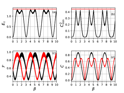
Figure 3: Dynamics of the quantities $E_{\tau}$, $\mathcal{C}_{\min}^{2}$, fidelity and concurrence as a function of $\beta$. In panels (a) and (b) we show $E_{\tau}$ and $C_{min}^{2}$. Notice that both curves peak around $\beta=1,2,4,5,7,8...$, getting close to their maximum values $4/3$ and $4/9$ (red line), respectively. This suggests the formation of maximum entangled $|W\rangle$ state at these particular $\beta$ values. In panel (c) we show the fidelity for the target state $|\psi(\alpha_{\mathrm{max}})\rangle$ with both phase signs $e^{i\frac{2\pi}{3}}$ (red curve) and $e^{-i\frac{2\pi}{3}}$ (black curve). Note that $\mathcal{F}\approx 1$ at the same $\beta$ values where $E_{\tau}$ and $C_{min}^{2}$ peaks occur, thus revealing the $|W\rangle$ states being formed. In panel (d) we show both the concurrences between qubits $BC$ ($C_{BC}$, black line) and qubits $AB$ ($C_{AB}$, red line). The peaks observed for $C_{AB}$ and $C_{BC}$ indicate the formation of partially bipartite entanglement. For instance, the peaks of $C_{BC}$ (black line) suggest the formation of a partially entangled state between qubits $B$ and $C$. Analogously, the peaks of $C_{AB}$ (red line) indicate the formation of partial entanglement between qubits $A$ and $B$. Parameters: $g=0.1\omega$, $\delta=0.1\omega$ and $t=0.005\omega$.

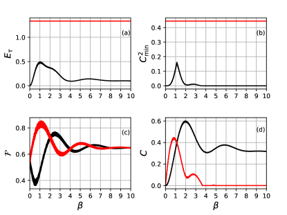
Figure 4: Dynamics of $E_{\tau}$, $\mathcal{C}_{\min}^{2}$, fidelity and concurrences against $\beta$ in the presence of dephasing in qubit $A$. The quantities (a) $E_{\tau}$ and (b) $C^{2}_{min}$ are suppressed due to dephasing, indicating that tripartite entanglement is quite sensible to dephasing in one of the three qubits. The fidelity in panel (c) shows damped oscillation with only the first peak becoming close to the target $|W\rangle$ state. In panel (d) we show both the concurrences $C_{AB}$ (red line) and $C_{BC}$ (black line). As a result of dephasing in qubit $A$, the concurrence $C_{AB}$ is suppressed. In contrast, $C_{BC}$ is preserved for longer times. Parameters: $g=0.1\omega$, $\delta=0.1\omega$ and $t=0.005\omega$, $\Gamma=1\cdot 10^{-4}\omega$ ($0.5$GHz).

V Conclusion

We investigate how the coupling between charge degrees of freedom and vibrational modes can yield to the formation of highly entangled $\mathinner{|{W}\rangle}$ states. We numerically calculate quantities such as $E_{\tau}$ and $\mathcal{C}_{\min}^{2}$, that peak on the formatio of $\mathinner{|{W}\rangle}$ states. Based on perturbation theory and the Lang-Firsov transformation, we derive analytical expressions that recover our full numerical calculation, thus providing a simple physical picture of the complex dynamics driven by the many body interaction. In particular, we analytically predict with great accuracy the times in which the $\mathinner{|{W}\rangle}$ state is being formed. Additionally, via concurrence calculation we find partial entanglement between subsystems composed of only two electronic qubits, i.e., tracing out one of the qubits. We show that even in the presence of dephasing mechanisms taken in one of the qubits, a partial entanglement between the other two qubits is preserved for relatively large times, thus revealing the robustness of the present system against local dephasing processes.

Supplemental Material

The model presented in Eqs.(2)-(4) is suitable in the description of quantum computation and quantum information, such as calculation of entanglement properties, as the subspaces and qubits structures are emphasized. However, if we are interested in quantum transport phenomena, it becomes more suitable to deal with second quantization formalism. The second quantization allows the inclusion in the computational basis states such as $\mathinner{|{vac}\rangle}$, i.e., the vacuum state, that can be experimentally achieved by draining all the particles of the system into nearby attached electrodes. Alternatively, we can have a state with all the electronic states being occupied due to charge injection from electrodes with high enough chemical potentials. In order to achieve such description we can rewrite our model Hamiltonian in its second quantized form

$$H_{dot} = \sum_{i=1}^{6}\varepsilon_{i}d_{i}^{\dagger}d_{i}+(t_{1}d_{1}^{\dagger}d_{2}+t_{2}d_{3}^{\dagger}d_{4}+t_{3}d_{5}^{\dagger}d_{6}+h.c.),$$

where $d_{i}$ ($d_{i}^{\dagger}$) annihilates (creates) one electron in quantum dot $i$. In this description each qubit is composed by two quantum dots, i.e., qubit A: dots 1-2, qubit B: dots 3-4 and qubit C: dots 5-6. Each quantum dot has a single energy level $\varepsilon_{i}$ and the dots in each qubit are coupled to each other via a hopping parameter $t_{i}$. For the bosonic subsystem we have

$$H_{b}=\omega_{1}b_{1}^{\dagger}b_{1}+\omega_{2}b_{2}^{\dagger}b_{2},$$ (45)

with $\omega_{i}$ being the energy of the $i$-th vibrational mode and $b_{i}$ ($b_{i}^{\dagger}$) the annihilation (creation) operator for the bosonic field. The electron-phonon coupling can be written in its standard form,footnote2

$$V = g_{1}d_{1}^{\dagger}d_{1}(b_{1}^{\dagger}+b_{1})+g_{2}d_{2}^{\dagger}d_{2}(b_{2}^{\dagger}+b_{2})$$ (46)

$$+ g_{1}d_{3}^{\dagger}d_{3}(b_{1}^{\dagger}+b_{1})+g_{2}d_{4}^{\dagger}d_{4}(b_{2}^{\dagger}+b_{2})$$

$$+ g_{1}d_{5}^{\dagger}d_{5}(b_{1}^{\dagger}+b_{1})+g_{2}d_{6}^{\dagger}d_{6}(b_{2}^{\dagger}+b_{2})$$

where $g_{i}$ gives the electron-phonon coupling strength. This equation is the second quantizad version of Eq. (4). Notice, though, that the operator in Eq. (46) belongs to a much larger Hilber space when compared to the one in Eq. (4), as each quantum dot can sustain two states, namely, no particle $\mathinner{|{1}\rangle}$ or one particle $\mathinner{|{0}\rangle}$. So for the electronic subspace we have $2^{6}$ possible states, contrasting to Eq. (4) where the qubits description provides $2^{3}$ available electronic configurations. The operators $d_{i}$ can be expressed in terms of Jordan-Wigner expansion, as described in Ref. [souza2017, ].

Here we simulate an experimental scenario where the molecular system is initially empty of particles, i.e., its initial quantum state $\mathinner{|{n_{1}n_{2}n_{3}n_{4}n_{5}n_{6}}\rangle}\otimes\mathinner{|{N_{1}N_{2}}\rangle}$ is given by $\mathinner{|{111111}\rangle}\otimes\mathinner{|{00}\rangle}$, with $n_{i}=1$ indicating no particle in $i$-th quantum dot and $N_{i}=0$ no excitation in the $i$-th bosonic bath. The quantum state that will evolve is then initialized with a pulse of gate voltage that controls the charge injection in each quantum dot. This kind of initialization can be experimentally implemented.shinkai2009 To this aim we apply the following Lindblad equation,lindblad1976

$$\dot{\rho}=-i[H_{0},\rho]-\frac{1}{2}\sum_{i=1}^{6}\Gamma_{i}[d_{i}d_{i}^{\dagger}\rho-d_{i}^{\dagger}\rho d_{i}+h.c.],$$ (47)

with $H_{0}=H_{dot}+V+H_{b}$. Notice that this Lindblad equation differs from the one in Eq. (43). Here it accounts for charge injection from reservoirs (leads) into the quantum dots, while in Eq. (43) it describes pure dephasing. We assume that $\Gamma_{i}$ is governed by external gate voltages that control the charge tunneling between leads and dots. In particular, we assume that only $\Gamma_{2}$, $\Gamma_{3}$ and $\Gamma_{5}$ assume nonzero values, with charges being injected in quantum dots $2$, $3$ and $5$. This gate pulse results in the following initialized state

$$\mathinner{|{\psi_{0}}\rangle}=\mathinner{|{100101}\rangle}\otimes\mathinner{|{00}\rangle}.$$ (48)

After the initialization pulse, the system evolves reaching highly entangled states. Here in particular we will focus on the formation of the same states found in Eq. (38), that correspond to the peaks observed in Fig. 3(c). In the present notation the target state can be written as

$$\mathinner{|{\phi_{\pm}}\rangle}=[\mathinner{|{100101}\rangle}+e^{\pm i2\pi/3}(\mathinner{|{011001}\rangle}+\mathinner{|{010110}\rangle})]\otimes\mathinner{|{00}\rangle}/\sqrt{3}.$$ (49)

Defining the target state as $\sigma_{\mathrm{tar}}=\mathinner{|{\phi_{\pm}}\rangle}\mathinner{\langle{\phi_{\pm}}|}$ we compute the fidelity $\mathcal{F}=\mathrm{Tr}\{\sigma_{\mathrm{tar}}\rho(t)\}$, with the density matrix provided by Eq. (47).

Figure (5) shows $\mathcal{F}$ against $\beta$ after the system being initialized by a gate pulse (blue line). Both phase signs are shown, $e^{-i2\pi/3}$ (black line) and $e^{+i2\pi/3}$ (red line). Notice that these results are very similar to the ones found in Fig. 3(c). The main contrast is the maximum value reached by the fidelity in the presence of initialization pulse, which is lower when compared to the case illustrated in Fig. 3(c). This fidelity suppression is related to the initialization procedure that imposes some decoherence to the system. To inject charge into the quantum system we need to open it during some time interval, by connecting the molecular structure to charge reservoirs. This coupling between system and charge reservoirs (leads) brings unavoidable decoherences that are reflected in a reduction of the fidelity degree in the subsequent quantum evolution.

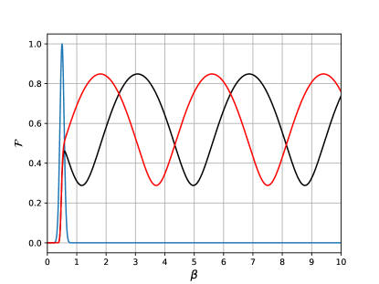
Figure 5: Fidelity against $\beta$ in the presence of a gate voltage pulse (blue line) that initializes the quantum state. Both signs of the relative phases of the target state $\mathinner{|{\phi}\rangle}_{\pm}$ are considered, $e^{-i2\pi/3}$ (black line) and $e^{+i2\pi/3}$ (red line). The fidelity peak is reduced when compared to the result in Fig 3(c), due to the decoherence imposed by the charge injection occuring in the initialization gate pulse. Parameters: $g=0.1\omega$, $\delta=0.1\omega$ and $t=0.005\omega$.