On the unification of the graph edit distance and graph matching problems

Abstract

Error-tolerant graph matching gathers an important family of problems. These problems aim at finding correspondences between two graphs while integrating an error model. In the Graph Edit Distance (GED) problem, the insertion/deletion of edges/nodes from one graph to another is explicitly expressed by the error model. At the opposite, the problem commonly referred to as “graph matching” does not explicitly express such operations. For decades, these two problems have split the research community in two separated parts. It resulted in the design of different solvers for the two problems. In this paper, we propose a unification of both problems thanks to a single model. We give the proof that the two problems are equivalent under a reformulation of the error models. This unification makes possible the use on both problems of existing solving methods from the two communities.

Keywords— Graph edit distance, graph matching, error-correcting graph matching, discrete optimization

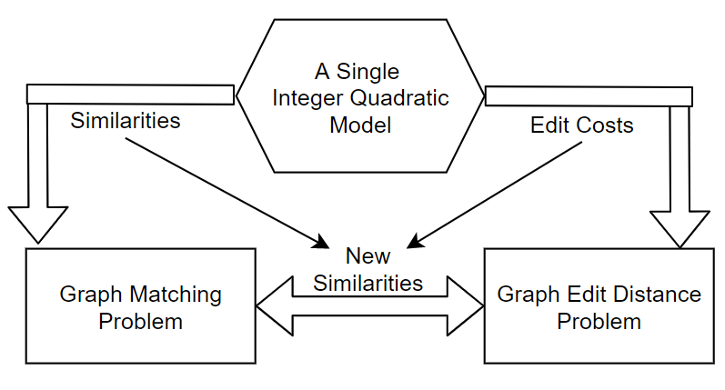
Graphical Abstract

1 Introduction

Graphs are frequently used in various fields of computer science, since they constitute a universal modeling tool which allows the description of structured data. The handled objects and their relations are described in a single and human-readable formalism. Hence, tools for graphs supervised classification and graph mining are required in many applications such as pattern recognition (Riesen, 2015), chemical components analysis, transfer learning (Das and Lee, 2018). In such applications, comparing graphs is of first interest. The similarity or dissimilarity between two graphs requires the computation and the evaluation of the “best” matching between them. Since exact isomorphism rarely occurs in pattern analysis applications, the matching process must be error-tolerant, i.e., it must tolerate differences on the topology and/or its labeling. The Graph Edit Distance (GED)(Riesen, 2015) problem and the Graph Matching problem (GM) (Swoboda et al., 2017) provide two different error models. These two problems have been deeply studied but they have split the research community into two groups of people developing separately quite different methods.

In this paper, we propose to unify the GED problem and the GM problem in order to unify the work force in terms of methods and benchmarks. We show that the GED problem can be equivalent to the GM problem under certain (permissive) conditions. The paper is organized as follows: Section 2, we give the definitions of the problems. Section 3, the state of the art on GM and GED is presented along with the literature comparing GED and GM to other problems. Section 4, a specific related work is detailed since it is the basement of our reasoning. Section 5, our proposal is described and a proof is given. Section 6, experimental results are presented to validate empirically our proposal. Finally, conclusions are drawn.

2 Definitions and problems

In this section, we define the problems to be studied. An attributed graph is considered as a set of 4 tuples ($V$,$E$,$\mu$,$\zeta$) such that: $G$ = ($V$,$E$,$\mu$,$\zeta$). $V$ is a set of vertices. $E$ is a set of edges such as $E\subseteq V\times V$. $\mu$ is a vertex labeling function which associates a label to a vertex. $\zeta$ is an edge labeling function which associates a label to an edge.

2.1 Graph matching problem

The objective of graph matching is to find correspondences between two attributed graphs $G_{1}$ and $G_{2}$. A solution of graph matching is defined as a subset of possible correspondences $\mathcal{Y}\subseteq V_{1}\times V_{2}$, represented by a binary assignment matrix $Y\in\{0,1\}^{n1\times n2}$, where $n1$ and $n2$ denote the number of nodes in $G_{1}$ and $G_{2}$, respectively. If $u_{i}\in V_{1}$ matches $v_{k}\in V_{2}$, then $Y_{i,k}=1$, and $Y_{i,k}=0$ otherwise. We denote by $y\in\{0,1\}^{n1.n2}$, a column-wise vectorized replica of $Y$. With this notation, graph matching problems can be expressed as finding the assignment vector $y^{*}$ that maximizes a score function $S(G_{1},G_{2},y)$ as follows:

Model 1.

Graph matching model (GMM)

$$y^{*}= \underset{y}{\mathrm{argmax}}\quad S(G_{1},G_{2},y)$$ (1a)

subject to $$y_{i,k}\in\{0,1\}\quad\forall(u_{i},v_{k})\in V_{1}\times V_{2}$$ (1b)

$$\sum_{u_{i}\in V_{1}}y_{i,k}\leq 1\quad\forall v_{k}\in V_{2}$$ (1c)

$$\sum_{v_{k}\in V_{2}}y_{i,k}\leq 1\quad\forall u_{i}\in V_{1}$$ (1d)

where equations (1c),(1d) induces the matching constraints, thus making $y$ an assignment vector.

The function $S(G_{1},G_{2},y)$ measures the similarity of graph attributes, and is typically decomposed into a first order similarity function $s(u_{i}\to v_{k})$ for a node pair $u_{i}\in V_{1}$ and $v_{k}\in V_{2}$, and a second-order similarity function $s(e_{ij}\to e_{kl})$ for an edge pair $e_{ij}\in E_{1}$ and $e_{kl}\in E_{2}$. Thus, the objective function of graph matching is defined as:

$$S(G_{1},G_{2},y)= \sum_{u_{i}\in V_{1}}\sum_{v_{k}\in V_{2}}s(u_{i}\to v_{k})\cdot y_{i,k}$$ (2)

$$+\sum_{e_{ij}\in E_{1}}\sum_{e_{kl}\in E_{2}}s(e_{ij}\to e_{kl})\cdot y_{ik}\cdot y_{jl}$$

In essence, the score accumulates all the similarity values that are relevant to the assignment. The GM problem has been proven to be $\mathcal{NP}$-hard by (Garey and Johnson, 1979).

2.2 Graph Edit Distance

The graph edit distance (GED) was first reported in (Tsai et al., 1979). GED is a dissimilarity measure for graphs that represents the minimum-cost sequence of basic editing operations to transform a graph into another graph by means classically included operations: insertion, deletion and substitution of vertices and/or edges. Therefore, GED can be formally represented by the minimum cost edit path transforming one graph into another. Edge operations are taken into account in the matching process when substituting, deleting or inserting their adjacent vertices. From now on and for simplicity, we denote the substitution of two vertices $u_{i}$ and $v_{k}$ by ($u_{i}\to v_{k}$), the deletion of vertex $u_{i}$ by ($u_{i}\to\epsilon$) and the insertion of vertex $v_{k}$ by ($\epsilon\to v_{k}$). Likewise for edges $e_{ij}$ and $e_{kl}$, ($e_{ij}\to e_{kl}$) denotes edges substitution, ($e_{ij}\to\epsilon$) and ($\epsilon\to e_{kl}$) denote edges deletion and insertion, respectively.

An edit path ($\lambda$) is a set of edit operations $o$. This set is referred to as Edit Path and it is defined in Definition 1.

Definition 1.

Edit Path
A set $\lambda=\{o_{1},\cdots,o_{k}\}$ of $k$ edit operations $o$ that transform $G_{1}$ completely into $G_{2}$ is called an (complete) edit path.

Let $c(o)$ be the cost function measuring the strength of an edit operation $o$. Let $\Gamma(G_{1},G_{2})$ be the set of all possible edit paths ($\lambda$). The graph edit distance problem is defined by Problem 3.

Problem 1.

Graph Edit Distance
Let $G_{1}$ = ($V_{1}$,$E_{1}$,$\mu_{1}$,$\zeta_{1}$) and $G_{2}$ = ($V_{2}$,$E_{2}$,$\mu_{2}$,$\zeta_{2}$) be two graphs, the graph edit distance between $G_{1}$ and $G_{2}$ is defined as:

$$d_{min}(G_{1},G_{2})=\min_{\lambda\in\Gamma(G_{1},G_{2})}\sum_{o\in\lambda}{c(o)}$$ (3)

The GED problem is a minimization problem and $d_{min}$ is the best distance. In its general form, the GED problem (Problem 3) is very versatile. The problem has to be refined to cope with the constraints of an assignment problem. First, let us define constraints on edit operations $(o_{i})$ in Definition 2.

Definition 2.

Edit operations constraints

1. Deleting a vertex implies deleting all its incident edges.

2. Inserting an edge is possible only if the two vertices already exist or have been inserted.

3. Inserting an edge must not create more than one edge between two vertices.

Second, let us define constraints on edit paths $(\lambda$) in Definition 3. This type of constraint prevents the edit path to be composed of an infinite number of edit operations.

Definition 3.

Edit path constraints

1. $k$ is a finite positive integer.

2. A vertex/edge can have at most one edit operation applied on it.

Finally, let us define the topological constraint in Definition 4. This type of constraints avoids edges to be matched without respect to their adjacent vertices.

Definition 4.

Topological constraint
The topological constraint implies that matching (substituting) two edges $(u_{i},u_{j})\in E_{1}$ and $(v_{k},v_{l})\in E_{2}$ is valid if and only if their incident vertices are matched $(u_{i}\to v_{k})$ and $(u_{j}\to v_{l})$.

An important property of the GED can be inferred from the topological constraint defined in Definition 4.

Property 1.

The edges matching are driven by the vertices matching

Assuming that constraint defined in Definition 4 is satisfied then three cases can appear :
Case 1: If there is an edge $e_{ij}$ = $(u_{i},u_{j})\in E_{1}$ and an edge $e_{kl}$ = $(v_{k},v_{l})\in E_{2}$, edges substitution between $(u_{i},u_{j})$ and $(v_{k},v_{l})$ is performed (i.e., ($e_{ij}\to e_{kl}$)).

Case 2: If there is an edge $e_{ij}$ = $(u_{i},u_{j})\in E_{1}$ and there is no edge between $v_{k}$ and $v_{l}$ then an edge deletion of $(u_{i},u_{j})$ is performed (i.e., ($e_{ij}\to\epsilon$)).
Case 3: If there is no edge between $u_{i}$ and $u_{j}$ and there is an edge between and an edge $e_{kl}$ = $(v_{k},v_{l})\in E_{2}$ then an edge insertion of $(v_{k},v_{l})$ is performed (i.e., ($\epsilon\to e_{kl}$)).

The GED problem defined in Problem 3 and refined with constraints defined in Definitions 2, 3 and 4 is referred in the literature and in this paper as the GED problem. The GED problem has been proven to be $\mathcal{NP}$-hard by (Zeng et al., 2009).

2.3 Related problems and models

GED and GM problems fall into the family of error-tolerant graph matching problems. GED and GM problems can be equivalent to another problem called Quadratic Assignment Problem (QAP) (Bougleux et al., 2017; Cho et al., 2013). In addition, GED and GM problems can be equivalent to a constrained version of the Maximum a posteriori (MAP)-inference problem of a Conditional Random Field (CRF) (Swoboda et al., 2017). All these problems can be expressed by mathematical models. A mathematical model is composed of variables, constraints and an objective functions. A single problem can be expressed by many different models. An Integer Quadratic Program (IQP) is a model with a quadratic objective function of the variables and linear constraints of the variables. We chose to present the GM problem as an IQP (Model 1). At the opposite, an Integer Linear Program (ILP) is a mathematical model where the objective function is a linear combination of the variables. The objective function is constrained by linear combinations of the variables.

3 State of the art

In this section, the state of the art is presented. First, the solution methods for GED and GM are described. Finally, papers comparing GED to other matching problems are mentioned.

3.1 State of the art on GM and GED

The GED and GM problems have been proven to be $\mathcal{NP}$-hard. So, unless $\mathcal{P}=\mathcal{NP}$, solving the problem to optimality cannot be done in polynomial time of the size of the input graphs. Consequently, the runtime complexity of exact methods is not polynomial but exponential with respect to the number of vertices of the graphs. On the other hand, heuristics are used when the demand for low computational time dominates the need to obtain optimality guarantees.

GM methods

Many solver paradigms were put to the test for GM. These include relaxations based on Lagrangean decompositions (Swoboda et al., 2017; Torresani et al., 2013), convex/concave quadratic (Liu and Qiao, 2014) (GNCCP) and semi-definite programming (Schellewald and Schnörr, 2005) , which can be used either directly to obtain approximate solutions or just to provide lower bounds. To tighten these bounds several cutting plane methods were proposed (Bazaraa and Sherali, 1982). On the other side, various primal heuristics, both (i) deterministic, such as graduated assignment methods (Gold and Rangarajan, 1996), fixed point iterations (Leordeanu et al., 2009) (IPFP), spectral technique and its derivatives (Cour et al., 2007; Leordeanu and Hebert, 2005) and (ii) non-deterministic (stochastic), like random walk (Cho et al., 2010) were proposed to provide approximate solutions to the problem. Many of these methods were published in TPAMI, NIPS, CVPR, ICCV.

GED methods

Exact GED algorithms were proposed based on tree search (Tsai et al., 1979; Riesen et al., 2007; Abu-Aisheh et al., 2015). Another way to build exact methods is to model the problem by Integer Linear Programs. Then, a black box solver is used to obtain solutions (Justice and Hero, 2006; Lerouge et al., 2017). In addition, the GED community worked on simplifications of the GED problem to the Linear Sum Assignment Problem (LSAP) (Bougleux et al., 2017; Serratosa, 2015; Riesen and Bunke, 2009). The GED problem was modeled as a QAP (Bougleux et al., 2017). Let us named this model GEDQAP. The GEDQAP model has extra variables to cope with the insertion and deletions cases and all costs are represented by a $(|V_{1}|+|V_{2}|)^{2}\times(|V_{1}|+|V_{2}|)^{2}$ matrix $D$. The cost matrix $D$ can be decomposed as follows into four blocks of size $(|V_{1}|+|V_{2}|)\times(|V_{1}|+|V_{2}|)$. The left upper block of the matrix $D$ contains all possible edge substitutions, the diagonal of the right upper matrix represents the cost of all possible edge deletions and the diagonal of the bottom left corner contains all possible edge insertions. Finally, the bottom right block elements cost is set to a large constant $w$ which concerns the matching of $\epsilon-\epsilon$ edges. The GEDQAP model has $(|V_{1}|+|V_{2}|)^{2}$ variables and $(|V_{1}|+|V_{2}|)+(|V_{1}|+|V_{2}|)$ constraints. The cost matrix size is $(|V_{1}|+|V_{2}|)^{2}\times(|V_{1}|+|V_{2}|)^{2}$. Based on this GEDQAP model, modified versions of IPFP (Bougleux et al., 2017) and GNCCP (Bougleux et al., 2017) were proposed. Finally, many GED methods were published in PRL, PR, Image and Vision Computing, GbR, SSPR.

3.2 State of the art on comparing GED problems to others

Neuhaus and Bunke (Neuhaus and Bunke., 2007) have shown that if each operation cost satisfies the criteria of a distance (positivity, uniqueness, symmetry, triangular inequality) then the edit distance defines a metric between graphs and it can be inferred that if $GED(G_{1},G_{2})=0\Leftrightarrow G_{1}=G_{2}$. Furthermore, it has been shown that standard concepts from graph theory, such as graph isomorphism, subgraph isomorphism, and maximum common subgraph, are special cases of the GED problem under particular cost functions (Bunke, 1997, 1999; Brun et al., 2012).

Deadlocks, contributions and motivations

From the literature, two main deadlocks can be drawn. First, GED and GM problems split the research community in two parts. People working on GED do not work on GM and vice and versa. They do not contribute to the same journals and conferences. Second, these two communities do not use the same methods to solve their problem while they have mainly the same applications fields (computer vision, chemoinformatics, …). Researchers working on GM problems have concentrated their efforts on the QAP and MAP-inference solvers (Frank-Wolfe like methodology (Leordeanu et al., 2009; Liu and Qiao, 2014), Lagrangian decomposition methods (Swoboda et al., 2017; Torresani et al., 2013), …). On the other hand, the community working on the GED problem has favored LSAP-based and tree-based methods.

Our motivation is to gather people working on GED and GM problems because methods and benchmarks built from one community could help the other. A first step forward has been done by (Bougleux et al., 2017) by modelling the GED problem as a specific QAP and using modified solvers from the graph matching community. However, our proposal stands apart from their work because we propose a single model to express the GM and the GED problems. In this direction, we propose more investigations to compare GED and GM problems. We propose a theoretical study to relate GM and GED problems. Our contribution is to prove that GED and GM problems are equivalent in terms of solutions under a reformulation of the similarity function. Consequently, all the methods solving the GM problem can be used to solve the GED problems.

4 Related works: Integer Linear Program for GED

In (Lerouge et al., 2017), an ILP was proposed to model the GED problem. This model will play an important role in our proposal so we propose to give a brief definition of this model. For each type of edit operation, a set of corresponding binary variables is defined in Table 1.

Table 1: Definition of binary variables of the ILP.

Name	Card	Role
$y_{i,k}$	$\forall(u_{i},v_{k})\in V_{1}\times V_{2}$	=1 if $u_{i}$ is substituted with $v_{k}$
$z_{ij,kl}$	$\forall(e_{ij},e_{kl})\in E_{1}\times E_{2}$	=1 if $e_{ij}$ is substituted with $e_{kl}$
$a_{i}$	$\forall u_{i}\in V_{1}$	=1 if $u_{i}$ is deleted from $G_{1}$
$b_{ij}$	$\forall e_{ij}\in E_{1}$	=1 if $e_{ij}$ is deleted from $G_{1}$
$g_{k}$	$\forall v_{k}\in V_{2}$	=1 if $v_{k}$ is inserted in $G_{1}$
$h_{kl}$	$\forall e_{kl}\in E_{2}$	=1 if $e_{kl}$ is inserted in $G_{1}$

The objective function (4) is the overall cost induced by an edit path $({y},{z},{a},{b},{g},{h})$ that transforms a graph $G_{1}$ into a graph $G_{2}$. In order to get the graph edit distance between $G_{1}$ and $G_{2}$, this objective function must be minimized.

$$C({y,z,a,b,g,h})=\Biggl{(}\sum_{u_{i}\in V_{1}}\sum_{v_{k}\in V_{2}}c(u_{i}\rightarrow v_{k})\cdot y_{i,k}$$ (4)

$$+\sum_{e_{ij}\in E_{1}}\sum_{e_{kl}\in E_{2}}c(e_{ij}\rightarrow e_{kl})\cdot z_{ij,kl}+\sum_{u_{i}\in V_{1}}c(u_{i}\rightarrow\epsilon)\cdot a_{i}$$

$$+\sum_{v_{k}\in V_{2}}c(\epsilon\rightarrow v_{k})\cdot g_{k}+\sum_{e_{ij}\in E_{1}}c(e_{ij}\rightarrow\epsilon)\cdot b_{ij}$$

$$+\sum_{e_{kl}\in E_{2}}c(\epsilon\rightarrow e_{kl})\cdot h_{kl}\Biggr{)}$$

Now, the constraints are presented. They are mandatory to guarantee that the admissible solutions of the ILP are edit paths that transform $G_{1}$ in $G_{2}$. The constraint (5a) ensures that each vertex of $G_{1}$ is either mapped to exactly one vertex of $G_{2}$ or deleted from $G_{1}$, while the constraint (5b) ensures that each vertex of $G_{2}$ is either mapped to exactly one vertex of $G_{1}$ or inserted in $G_{1}$:

$$a_{i}+\sum_{v_{k}\in V_{2}}y_{i,k}=1\quad\forall u_{i}\in V_{1}$$ (5a)

$$g_{k}+\sum_{u_{i}\in V_{1}}y_{i,k}=1\quad\forall v_{k}\in V_{2}$$ (5b)

The same applies for edges:

$$b_{ij}+\sum_{e_{kl}\in E_{2}}z_{ij,kl}=1\quad\forall e_{ij}\in E_{1}$$ (6a)

$$h_{kl}+\sum_{e_{ij}\in E_{1}}z_{ij,kl}=1\quad\forall e_{kl}\in E_{2}$$ (6b)

The topological constraints defined in Definition 4 can be expressed with the following constraints (7) and (8):

$e_{ij}$ and $e_{kl}$ can be mapped only if their head vertices are mapped:

$$z_{ij,kl}\leq y_{i,k}\quad\forall(e_{ij},e_{kl})\in E_{1}\times E_{2}$$ (7)

$e_{ij}$ and $e_{kl}$ can be mapped only if their tail vertices are mapped:

$$z_{ij,kl}\leq y_{j,l}\quad\forall(e_{ij},e_{kl})\in E_{1}\times E_{2}$$ (8)

The insertions and deletions variables $a$, $b$, $g$ and $h$ help the reader to understand how the objective function and the constraints were obtained, but they are unnecessary to solve the GED problem. In the equation (4), the variables ${a},{b},{g}\text{ and }{h}$ are replaced by their expressions deduced from the equations (5a), (5b), (6a) and (6b). For instance, from the equation (5a), the variable $a$ is deduced: $a_{i}=1-\sum_{v_{k}\in V_{2}}y_{i,k}$ and replaced in the equation (4), the part of the objective function concerned by variable $a$ becomes:

$$\sum_{u_{i}\in V_{1}}c(u_{i}\rightarrow\epsilon)\cdot a_{i}= \sum_{u_{i}\in V_{1}}c(u_{i}\rightarrow\epsilon)$$ (9)

$$+\sum_{u_{i}\in V_{1}}\sum_{v_{k}\in V_{2}}-c(u_{i}\rightarrow\epsilon).y_{i,k}$$

Consequently, a new objective function is expressed as follows:

$$C^{\prime}({y,z})= \gamma+\sum_{u_{i}\in V_{1}}\sum_{v_{k}\in V_{2}}\Bigl{(}c(u_{i}\rightarrow v_{k})$$ (10)

$$-c(u_{i}\rightarrow\epsilon)-c(\epsilon\rightarrow v_{k})\Bigr{)}\cdot y_{i,k}$$

$$+\sum_{e_{ij}\in E_{1}}\sum_{e_{kl}\in E_{2}}\Bigl{(}c(e_{ij}\rightarrow e_{kl})$$

$$-c(e_{ij}\rightarrow\epsilon)-c(\epsilon\rightarrow e_{kl})\Bigr{)}\cdot z_{ij,kl}$$

$$\text{with }\gamma= \sum_{u_{i}\in V_{1}}c(u_{i}\to\epsilon)+\sum_{v_{k}\in V_{2}}c(\epsilon\to v_{k})$$

$$+\sum_{e_{ij}\in E_{1}}c(e_{ij}\to\epsilon)+\sum_{e_{kl}\in E_{2}}c(\epsilon\to e_{kl})$$

Equation (10) shows that the GED can be obtained without explicitly computing the variables ${a},{b},{g}\text{ and }{h}$. Once the formulation solved, all insertion and deletion variables can be a posteriori deduced from the substitution variables.

The vertex mapping constraints (5a) and (5b) are transformed into inequality constraints, without changing their role in the program. As a side effect, it removes the $a$ and $g$ variables from the constraints:

$$\sum_{v_{k}\in V_{2}}y_{i,k}\leq 1\quad\forall u_{i}\in V_{1}$$ (11)

$$\sum_{u_{i}\in V_{1}}y_{i,k}\leq 1\quad\forall v_{k}\in V_{2}$$ (12)

In fact, the insertions and deletions variables $a$ and $g$ of the equations (5a) and (5b) can be seen as slack variables to transform inequality constraints to equalities and consequently providing a canonical form. The entire formulation is called F2 and described as follows :

Model 2.

F2

$$\min_{{y,z}}C^{\prime}(y,z)$$ (13a)

subject to $$\sum_{v_{k}\in V_{2}}y_{i,k}\leq 1\quad\forall u_{i}\in V_{1}$$ (13b)

$$\sum_{u_{i}\in V_{1}}y_{i,k}\leq 1\quad\forall v_{k}\in V_{2}$$ (13c)

$$\sum_{e_{kl}\in E_{2}}z_{ij,kl}\leq y_{i,k}\quad\forall v_{k}\in V_{2},\forall e_{ij}\in E_{1}$$ (13d)

$$\sum_{e_{kl}\in E_{2}}z_{ij,kl}\leq y_{j,l}\quad\forall v_{l}\in V_{2},\forall e_{ij}\in E_{1}$$ (13e)

with $$y_{i,k}\in\{0,1\}\quad\forall(u_{i},v_{k})\in V_{1}\times V_{2}$$ (13f)

$$z_{ij,kl}\in\{0,1\}\quad\forall(e_{ij},e_{kl})\in E_{1}\times E_{2}$$ (13g)

$\gamma$ is not a function of $y$ and $z$. It does not impact the minimization problem. However, $\gamma$ is mandatory to obtain the GED value (i.e. $d_{min}(G_{1},G_{2})$ from Problem 3). The topological constraints (7) and (8) are expressed in another way and are replaced by the constraints (13d) and (13e).

5 Proposal on the unification of the two problems

In this paragraph, we propose to draw a relation between the graph matching and graph edit distance problems. Especially, we create a link between both problems through a change of similarity functions. Our proposal can be stated as follows:

Proposition 1.

GM and GED problems are equivalent in terms of solutions under a reformulation of the similarity function $s^{\prime}(u_{i}\to v_{k})=-\left(c(u_{i}\to v_{k})-c(u_{i}\to\epsilon)-c(\epsilon\to v_{k})\right)$ and $s^{\prime}(e_{ij}\to e_{kl})=-\left(c(e_{ij}\to e_{kl})-c(e_{ij}\to\epsilon)-c(\epsilon\to e_{kl})\right)$

To intuitively demonstrate the exactness of the proposition, we proceed as follows :

1. We start from the GED problem expressed by model F2 (see Model 13).

2. We link the similarity function $s$ with the cost function $c$ thanks to a new similarity function $s^{\prime}$.

3. With this similarity function $s^{\prime}$, we show that F2 turns to be a maximization problem and we call this new model F2’.

4. F2’ is modified by switching from a linear to a quadratic model called GMM’.

5. GMM’ is identical to GMM. It is sufficient to show that both models express the same problem, that is to say, the graph matching problem.

Proof.

1. By setting $d(u_{i}\to v_{k})=\Bigl{(}c(u_{i}\to v_{k})-c(u_{i}\to\epsilon)-c(\epsilon\to v_{k})\Bigr{)}$ and $d(e_{ij}\to e_{kl})=\Bigl{(}c(e_{ij}\to e_{kl})-c(e_{ij}\to\epsilon)-c(\epsilon\to e_{kl})\Bigr{)}$, we can rewrite the objective function of F2 as follows :

   $$C^{\prime}({y,z})= \gamma+\sum_{u_{i}\in V_{1}}\sum_{v_{k}\in V_{2}}d(u_{i}\to v_{k})\cdot y_{u_{i},v_{k}}$$ (14)

   $$+\sum_{e_{ij}\in E_{1}}\sum_{e_{kl}\in E_{2}}d(e_{ij}\to e_{kl})\cdot z_{ij,kl}$$

   $$\text{with }\gamma= \sum_{u_{i}\in V_{1}}c(u_{i}\to\epsilon)+\sum_{v_{k}\in V_{2}}c(\epsilon\to v_{k})$$

   $$+\sum_{e_{ij}\in E_{1}}c(e_{ij}\to\epsilon)+\sum_{e_{kl}\in E_{2}}c(\epsilon\to e_{kl})$$

2. $\gamma$ does not depend on variables so it does not impact the optimization problem. Therefore $\gamma$ can be removed.

3. By setting $s^{\prime}(u_{i}\to v_{k})=-d(u_{i}\to v_{k})=-\Bigl{(}c(u_{i}\to v_{k})-c(u_{i}\to\epsilon)-c(\epsilon\to v_{k})\Bigr{)}$ and similarly, $s^{\prime}(e_{ij}\to e_{kl})=-d(e_{ij}\to e_{kl})$, we can rewrite the objective function $C^{\prime}$ of the model F2 to obtain $S^{\prime}$.

   $$S^{\prime}({y,z})= \sum_{u_{i}\in V_{1}}\sum_{v_{k}\in V_{2}}s^{\prime}(u_{i}\to v_{k})\cdot y_{i,k}$$ (15)

   $$+\sum_{e_{ij}\in E_{1}}\sum_{e_{kl}\in E_{2}}s^{\prime}(e_{ij}\to e_{kl})\cdot z_{ij,kl}$$

4. In a general way, minimizing $f(x)$ is equivalent to maximize -$f(x)$. So, minimizing $C^{\prime}$ is equivalent to maximize $S^{\prime}$.

5. The linear objective function $S^{\prime}$ can be turned into a quadratic function by removing variables $z$ and replacing them by product of $y$ variables.

   $$S^{\prime\prime}(y)= \sum_{u_{i}\in V_{1}}\sum_{v_{k}\in V_{2}}s^{\prime}(u_{i}\to v_{k})\cdot y_{i,k}$$ (16)

   $$+\sum_{e_{ij}\in E_{1}}\sum_{e_{kl}\in E_{2}}s^{\prime}(e_{ij}\to e_{kl})\cdot y_{i,k}\cdot y_{j,l}$$

6. Topological constraints (Equations (13d) and (13e)) in F2 are not necessary anymore and they can be removed. The product of $y_{i,k}$ and $y_{j,l}$ is enough to ensure that an edge $e_{ij}\in E_{1}$ can be matched to an edge $e_{kl}\in E_{2}$ only if the head vertices $u_{i}\in V_{1}$ and $v_{k}\in V_{2}$, on the one hand, and if the tail vertices $u_{j}\in V_{1}$ and $v_{l}\in V_{2}$, on the other hand, are respectively matched.

7. We obtain the new model named GMM’:

   Model 3.

   GMM’

   $$y^{*}= \underset{y}{\mathrm{argmax}}\quad S^{\prime\prime}(y)$$ (17a)

   subject to $$\sum_{u_{i}\in V_{1}}y_{i,k}\leq 1\quad\forall v_{k}\in V_{2}$$ (17b)

   $$\sum_{v_{k}\in V_{2}}y_{i,k}\leq 1\quad\forall u_{i}\in V_{1}$$ (17c)

   with $$y_{i,k}\in\{0,1\}\quad\forall(u_{i},v_{k})\in V_{1}\times V_{2}$$ (17d)

8. Model GMM’ = Model GMM. This was to be demonstrated. Proposition 1 is right.

∎

Under the condition of Proposition 1, the optimal assignment obtains when solving the graph matching problem can be used to reconstruct an optimal solution of the GED problem. An instance of GED and an instance of GM are presented in Figure 1. Solutions of the GED instance are presented with respect to the cost function $c$ while the graph matching solutions are presented with respect to the similarity function $s^{\prime}$. The optimal matching of both instances are the same.

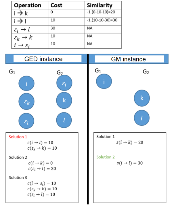
Figure 1: A comparison of the graph matching and GED problems when the similarity function $s^{\prime}(i\to k)=-\{c(i\to k)-c(i\to\epsilon)-c(\epsilon\to k)\}$

Model GMM’ has $|V_{1}|.|V_{2}|$ variables and $|V_{1}|+|V_{2}|$ constraints. Similarity functions can be represented by a similarity matrix $K$ of size is $|V_{1}|.|V_{2}|\times|V_{1}|.|V_{2}|$.

Proposition 1 is a first attempt toward the unification of two communities working respectively on GED and GM problems. All the methods solving the graph matching problem can be used to solve the graph edit distance problem under a specific similarity function $s^{\prime}(u_{i}\to v_{k})=-\Bigr{(}c(u_{i}\to v_{k})-c(u_{i}\to\epsilon)-c(\epsilon\to v_{k})\Bigr{)}$.

6 Experiments

In this section, we show the results of our numerical experiments to validate our proposal that the model GMM’ can model the GED problem if $s^{\prime}(i\to k)=-\{c(i\to k)-c(i\to\epsilon)-c(\epsilon\to k)\}$. We based our protocol on the ICPR GED contest. Among the data sets available, we chose the GREC data set for two reasons. First, graphs sizes range from 5 to 20 nodes and these sizes are amendable to compute optimal solutions. Second, the GREC cost function, defined in the contest, is complex enough to cover a large range of matching cases. This cost function is not a constant value and includes euclidean distances between point coordinates. The reader is redirected to (Abu-Aisheh et al., 2017) for the full definition of the cost function. From the GREC database, we chose the subset of graphs called ”MIXED” because it holds 10 graphs of various sizes. We computed all the pairwise comparisons to obtain 100 solutions. We compared the optimal solutions obtained by our Model GMM’ and the optimal solutions found by the straightforward ILP formulation called F1 (Lerouge et al., 2017). We computed the average difference between the GED values and the objective function values of our model GMM’. The average difference is exactly equal to zero. This result corroborates our theoretical statement. Detailed results and codes can be found on the website https://sites.google.com/view/a-single-model-for-ged-and-gm.

7 Conclusion

In this paper, an equivalence between graph matching and graph edit distance problems was proven under a reformulation of the similarity functions between nodes and edges. These functions should take into account explicitly the deletion and insertion costs. That’s the major difference between GM and GED problems. In the GED problem, costs to delete or to insert vertices or edges are explicitly introduced in the error model. On the other hand, deletion costs are implicitly set to a specific value (that is to say 0) in the GM problem. Many learning methods aim at learning edit costs (Serratosa, 2020; Martineau et al., 2020) or matching similarities (Zanfir and Sminchisescu, 2018; Caetano et al., 2007). Learned matching similarities may include implicitly deletion and insertion costs. Does it help the learning algorithm to learn separately insertion and deletion costs? That is still an open question. However, with this paper, we stand for a rapprochement of the research communities that work on learning graph edit distance and learning graph matching because edit costs can be hidden in the learned similarities.

References

- Riesen (2015) K. Riesen, Structural Pattern Recognition with Graph Edit Distance - Approximation Algorithms and Applications, Advances in Computer Vision and Pattern Recognition, Springer, 2015.
- Das and Lee (2018) D. Das, C. G. Lee, Sample-to-sample correspondence for unsupervised domain adaptation, Engineering Applications of Artificial Intelligence 73 (2018) 80 – 91.
- Swoboda et al. (2017) P. Swoboda, C. Rother, H. Abu Alhaija, D. Kainmuller, B. Savchynskyy, A study of lagrangean decompositions and dual ascent solvers for graph matching, in: CVPR, 2017.
- Garey and Johnson (1979) M. R. Garey, D. S. Johnson, Computers and Intractability; A Guide to the Theory of NP-Completeness, W. H. Freeman Co., USA, 1979.
- Tsai et al. (1979) W.-h. Tsai, S. Member, K.-s. Fu, Pattern Deformational Model and Bayes Error-Correcting Recognition System, IEEE Transactions on Systems, Man, and Cybernetics 9 (1979) 745–756.
- Zeng et al. (2009) Z. Zeng, A. K. H. Tung, J. Wang, J. Feng, L. Zhou, Comparing stars: On approximating graph edit distance, PVLDB 2 (2009) 25–36.
- Bougleux et al. (2017) S. Bougleux, L. Brun, V. Carletti, P. Foggia, B. Gauzere, M. Vento, Graph edit distance as a quadratic assignment problem, Pattern Recognition Letters 87 (2017) 38 – 46. Advances in Graph-based Pattern Recognition.
- Cho et al. (2013) M. Cho, K. Alahari, J. Ponce, Learning graphs to match, in: ICCV, 2013, pp. 25–32.
- Torresani et al. (2013) L. Torresani, V. Kolmogorov, C. Rother, A dual decomposition approach to feature correspondence, TPAMI 35 (2013) 259–271.
- Liu and Qiao (2014) Z. Liu, H. Qiao, Gnccp—graduated nonconvexityand concavity procedure, TPAMI 36 (2014) 1258–1267.
- Schellewald and Schnörr (2005) C. Schellewald, C. Schnörr, Probabilistic subgraph matching based on convex relaxation, in: A. Rangarajan, B. Vemuri, A. L. Yuille (Eds.), Energy Minimization Methods in Computer Vision and Pattern Recognition, Springer Berlin Heidelberg, Berlin, Heidelberg, 2005, pp. 171–186.
- Bazaraa and Sherali (1982) M. S. Bazaraa, H. D. Sherali, On the use of exact and heuristic cutting plane methods for the quadratic assignment problem, Journal of the Operational Research Society 33 (1982) 991–1003.
- Gold and Rangarajan (1996) S. Gold, A. Rangarajan, A graduated assignment algorithm for graph matching, TPAMI 18 (1996) 377–388.
- Leordeanu et al. (2009) M. Leordeanu, M. Hebert, R. Sukthankar, An integer projected fixed point method for graph matching and map inference, in: Y. Bengio, D. Schuurmans, J. D. Lafferty, C. K. I. Williams, A. Culotta (Eds.), NIPS, Curran Associates, Inc., 2009, pp. 1114–1122.
- Cour et al. (2007) T. Cour, P. Srinivasan, J. Shi, Balanced graph matching, in: B. Schölkopf, J. C. Platt, T. Hoffman (Eds.), NIPS, MIT Press, 2007, pp. 313–320.
- Leordeanu and Hebert (2005) M. Leordeanu, M. Hebert, A spectral technique for correspondence problems using pairwise constraints, in: ICCV, volume 2, 2005, pp. 1482–1489 Vol. 2.
- Cho et al. (2010) M. Cho, J. Lee, K. M. Lee, Reweighted random walks for graph matching, in: K. Daniilidis, P. Maragos, N. Paragios (Eds.), ECCV, Springer Berlin Heidelberg, Berlin, Heidelberg, 2010, pp. 492–505.
- Riesen et al. (2007) K. Riesen, S. Fankhauser, H. Bunke, Speeding up graph edit distance computation with a bipartite heuristic, in: Mining and Learning with Graphs, Proceedings, 2007.
- Abu-Aisheh et al. (2015) Z. Abu-Aisheh, R. Raveaux, J. Ramel, P. Martineau, An exact graph edit distance algorithm for solving pattern recognition problems, in: ICPRAM, 2015, pp. 271–278.
- Justice and Hero (2006) D. Justice, A. Hero, A binary linear programming formulation of the graph edit distance, TPAMI 28 (2006) 1200–1214.
- Lerouge et al. (2017) J. Lerouge, Z. Abu-Aisheh, R. Raveaux, P. Héroux, S. Adam, New binary linear programming formulation to compute the graph edit distance, Pattern Recognition 72 (2017) 254–265.
- Bougleux et al. (2017) S. Bougleux, B. Gaüzère, L. Brun, A hungarian algorithm for error-correcting graph matching, in: P. Foggia, C.-L. Liu, M. Vento (Eds.), Graph-Based Representations in Pattern Recognition, Springer International Publishing, Cham, 2017, pp. 118–127.
- Serratosa (2015) F. Serratosa, Computation of graph edit distance: Reasoning about optimality and speed-up, Image Vision Comput. 40 (2015) 38–48.
- Riesen and Bunke (2009) K. Riesen, H. Bunke, Approximate graph edit distance computation by means of bipartite graph matching, Image Vision Comput. 27 (2009) 950–959.
- Neuhaus and Bunke. (2007) M. Neuhaus, H. Bunke., Bridging the gap between graph edit distance and kernel machines., Machine Perception and Artificial Intelligence. 68 (2007) 17–61.
- Bunke (1997) H. Bunke, On a relation between graph edit distance and maximum common subgraph, Pattern Recognition Letters 18 (1997) 689–694.
- Bunke (1999) H. Bunke, Error correcting graph matching: On the influence of the underlying cost function, TPAMI 21 (1999) 917–922.
- Brun et al. (2012) L. Brun, B. Gaüzère, S. Fourey, Relationships between Graph Edit Distance and Maximal Common Unlabeled Subgraph, Technical Report, 2012.
- Abu-Aisheh et al. (2017) Z. Abu-Aisheh, B. Gauzere, S. Bougleux, et al, Graph edit distance contest: Results and future challenges, Pattern Recognition Letters 100 (2017) 96 – 103.
- Serratosa (2020) F. Serratosa, A general model to define the substitution, insertion and deletion graph edit costs based on an embedded space, Pattern Recognition Letters 138 (2020) 115 – 122.
- Martineau et al. (2020) M. Martineau, R. Raveaux, D. Conte, G. Venturini, Learning error-correcting graph matching with a multiclass neural network, Pattern Recognition Letters 134 (2020) 68 – 76.
- Zanfir and Sminchisescu (2018) A. Zanfir, C. Sminchisescu, Deep learning of graph matching, in: 2018 IEEE/CVF Conference on Computer Vision and Pattern Recognition, 2018, pp. 2684–2693.
- Caetano et al. (2007) T. S. Caetano, Li Cheng, Q. V. Le, A. J. Smola, Learning graph matching, in: 2007 IEEE 11th International Conference on Computer Vision, 2007, pp. 1–8.