Optimal Transmission of Multi-Quality Tiled 360 VR Video in MIMO-OFDMA Systems

Abstract

In this paper, we study the optimal transmission of a multi-quality tiled 360 virtual reality (VR) video from a multi-antenna server (e.g., access point or base station) to multiple single-antenna users in a multiple-input multiple-output (MIMO)-orthogonal frequency division multiple access (OFDMA) system. We minimize the total transmission power with respect to the subcarrier allocation constraints, rate allocation constraints, and successful transmission constraints, by optimizing the beamforming vector and subcarrier, transmission power and rate allocation. The formulated resource allocation problem is a challenging mixed discrete-continuous optimization problem. We obtain an asymptotically optimal solution in the case of a large antenna array, and a suboptimal solution in the general case. As far as we know, this is the first work providing optimization-based design for 360 VR video transmission in MIMO-OFDMA systems. Finally, by numerical results, we show that the proposed solutions achieve significant improvement in performance compared to the existing solutions.

I Introduction

By using an omnidirectional camera to capture a scene of interest in all directions at the same time, a 360 virtual reality (VR) can be generated. In many VR applications, e.g., VR gaming, VR concert, and VR military training, a 360 VR video has to be transmitted to multiple users simultaneously. Transmitting a 360 VR video over wireless networks enables users to experience immersive environments without geographical or behavioral restrictions. In this paper, the main focus is on optimally transmitting a 360 VR video in a multi-user wireless network.

A 360 VR video has a much larger size than a traditional video. When watching a 360 VR video, a user is perceiving it from only one viewing direction at any time, which corresponds to one part of the 360 VR video, known as field-of-view (FoV). Tiling technique is widely used to improve the transmission efficiency for 360 VR videos [1]. Transmitting the set of tiles which cover predicted FoVs can reduce the required communication resources, without affecting the quality of experience. When transmitting a tiled 360 VR video in a multi-user wireless network, if there exists a tile required by multiple users concurrently, multicast opportunities can be utilized to improve transmission efficiency. Recently, [2, 3, 4, 5, 6, 7] study streaming of a tiled 360 VR video from a single-antenna server to multiple single-antenna users in wireless networks, where multicast opportunities are exploited. In particular, in our previous works [2, 3], the optimal transmission of a single-quality tiled 360 VR video is studied. In practice, pre-encoding each tile into multiple representations with different quality levels allows quality adaptation according to users’ channel conditions. In [4, 5, 6, 7], the optimal transmission of a multi-quality tiled 360 VR video is considered, with the main focus on the optimization of quality level selection for each tile.

Despite the fruitful research in the literature, the performance of wireless transmission of a tiled 360 VR video is still limited. In fact, the results in [2, 3, 4, 5, 6, 7] all consider single-antenna servers, which cannot exploit the spatial degrees of freedom. The performance of wireless systems can be significantly improved by deploying multiple antennas at a server and designing efficient beamformers. Among various multi-antenna technologies, MIMO-OFDMA is the dominant air interface for 5G broadband wireless communications, as it can provide more reliable communications at high speeds. For instance, in [8, 9], the authors consider multi-group multicast in MIMO-OFDMA systems. Specifically, In [8], the subcarrier and power allocation is considered to maximize the system sum rate. However, the solution proposed in [8] is heuristic, and hence has no performance guarantee. In [9], the authors study the optimization of beamformers to minimize the total transmission power, and obtain a stationary point of the beamforming design problem based on successive convex approximation. Note that in [9], messages on each subcarrier have different beamformers, resulting in a substantial increase in the number of variables and hence the computational complexity for solving the optimization problem.

In this paper, we consider the optimal transmission of a multi-quality tiled 360 VR video in a MIMO-OFDMA system. With more advanced physical layer techniques than those in [2, 3, 4, 5, 6, 7], we expect the stringent requirements for 360 VR video transmission to be better satisfied. We minimize the total transmission power by optimizing the beamforming vectors and subcarrier, transmission power, and rate allocation, under the subcarrier allocation constraints, rate allocation constraints, and successful transmission constraints. This problem is a mixed discrete-continuous optimization problem, and is very challenging. We obtain its asymptotically optimal solution in the special case of a large antenna array, by exploiting decomposition, continuous relaxation, and Karush-Kuhn-Tucker (KKT) conditions. We also obtain a suboptimal solution in the general case, applying continuous relaxation and difference of convex (DC) programming. Note that the transmission of a tiled 360 VR video in this paper can be viewed as multi-group multicast. Previous works studying multi-group multicast in MIMO-OFDMA systems do not investigate the special case of a large antenna array where an asymptotically optimal solution can be obtained [8, 9]. Note that the proposed formulation in this paper, with one beamforming vector for each subcarrier, can achieve the same performance as the formulation in [9] but with much lower computational complexity in the general case. Finally, numerical results show substantial gains achieved by the proposed solutions over existing schemes.

II System Model

We consider the streaming of a multi-quality tiled 360 VR video from a server (e.g., access point or base station) to $K$ users in an MIMO-OFDMA system as illustrated in Fig. 1. The server is equipped with $M$ transmit antennas and each user wears a single-antenna VR headset. Denote $\mathcal{K}\triangleq\{1,\ldots,K\}$ as the set of user indices. When a VR user is interested in one viewing direction of a 360 VR video, the user watches a rectangular FoV of size $F_{h}\times F_{v}$ (in rad$\times$rad), the center of which is referred to as the viewing direction. In addition, a user can freely switch views when watching a 360 VR video.

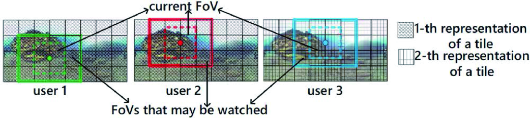
(a) Multi-quality tiled 360 VR video required by multiple users.

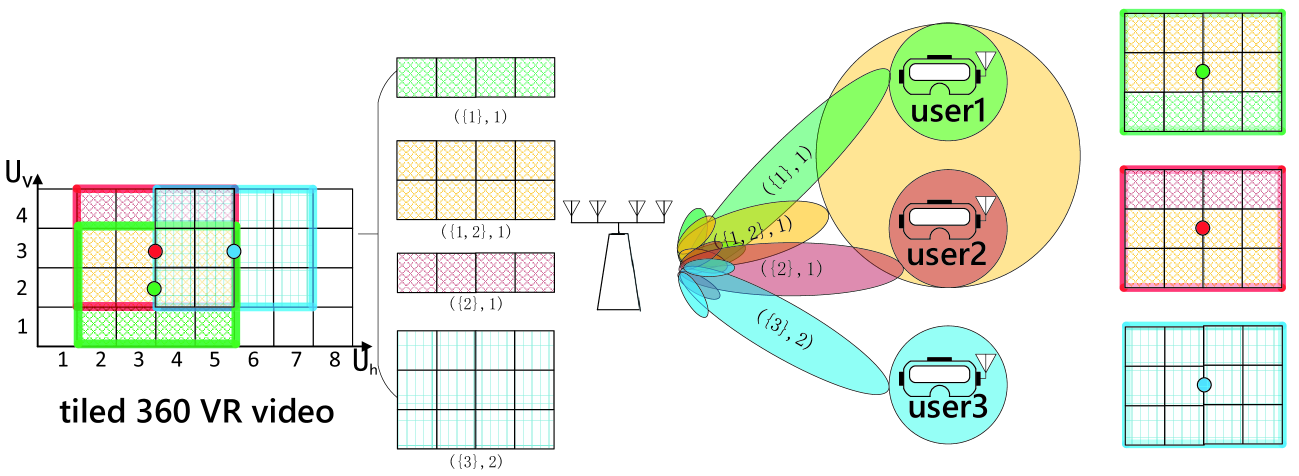
(b) Transmission of a multi-quality tiled 360 VR video.

Figure 1: System model of transmission of a multi-quality tiled 360 VR video. $K=3$, $\mathbf{r}=(1,1,2),$ $U_{h}\times U_{v}=8\times 4$, $M=4$, $\mathcal{G}_{1}=\{(2,1),(3,1),(4,1),(5,1),(2,2),(3,2),(4,2),(5,2),(2,3),(3,3)$, $(4,3),(5,3)\}$, $\mathcal{G}_{2}=\{(2,2),(3,2),(4,2),(5,2),(2,3),(3,3),(4,3)$, $(5,3),(2,4),(3,4),(4,4),(5,4)\}$, $\mathcal{G}_{3}=\{(4,2),(5,2),(6,2),(7,2)$, $(4,3),(5,3),(6,3),(7,3),(4,4),(5,4),(6,4),(7,4)\}$, $\mathcal{I}=\{\{1\},\{2\},\{3\},\{1,3\},\{2,3\},\{1,2,3\}\}$, $\mathcal{P}_{\{1\}}=\{(2,1),(3,1),(4,1),(5,1)\}$, $\mathcal{P}_{\{2\}}=\{(2,4),(3,4)\}$, $\mathcal{P}_{\{3\}}=\{(6,2),(6,3),(6,4),(7,2),(7,3),(7,4)\}$, $\mathcal{P}_{\{1,2\}}=\{(2,2),(2,3),(3,2),(3,3)\}$, $\mathcal{P}_{\{2,3\}}=\{(4,4),(5,4)\}$, $\mathcal{P}_{\{1,2,3\}}=\{(4,2),(4,3),(5,2),(5,3)\}$, $\mathcal{K}_{\{1\},1}=\{1\},$ $\mathcal{K}_{\{1,2\},1}=\{1,2\},$ $\mathcal{K}_{\{2\},1}=\{2\},$ $\mathcal{K}_{\{3\},2}=\{3\}.$

Tiling is adopted to improve transmission efficiency of the 360 VR video. In particular, the 360 VR video is divided into multiple rectangular segments of the same size, which are referred to as tiles. Let $U_{h}$ and $U_{v}$ denote the numbers of segments in each row and column, respectively. Define $\mathcal{U}_{h}\triangleq\{1,\ldots,U_{h}\}$ and $\mathcal{U}_{v}\triangleq\{1,\ldots,U_{v}\}$. The $(u_{h},u_{v})$-th tile is referred to as the tile in the $u_{h}$-th row and the $u_{v}$-th column, for all $u_{h}\in\mathcal{U}_{h}$ and $u_{v}\in\mathcal{U}_{v}$. Considering user heterogeneity (e.g., display resolutions of devices, channel conditions, etc.), each tile is pre-encoded into $L$ representations corresponding to $L$ quality levels using High Efficiency Video Coding (HEVC), as in Dynamic Adaptive Streaming over HTTP (DASH). Denote $\mathcal{L}\triangleq\{1,\ldots,L\}$ as the set of quality levels. For all $l\in\mathcal{L}$, the $l$-th representation of each tile corresponds to the $l$-th lowest quality. For ease of exposition, we assume that the encoding rates of the tiles with the same quality level are identical. Let $D_{l}$ (in bits/s) denote the encoding rate of the $l$-th representation of a tile. Note that $D_{1}<D_{2}<\ldots<D_{L}$. We consider the duration of the playback time of one group of pictures (GOP), over which the FoV of each user does not change. Let $r_{k}\in\mathcal{L}$ denote the quality level for the FoV of user $k\in\mathcal{K}$. Due to the video coding structure, $\mathbf{r}\triangleq(r_{k})_{k\in\mathcal{K}}$ should not change during the considered time duration.

As in [2, 3, 6], suppose the FoV of each user has been predicted and we focus on the transmission of a multi-quality tiled 360 VR video. Let $\mathcal{G}_{k}$ denote the set of indices of the tiles which need to be transmitted to user $k$ and let $\mathcal{G}\triangleq\bigcup_{k\in\mathcal{K}}\mathcal{G}_{k}$ denote the set of indices of the tiles which need to be transmitted considering all $K$ users. For all $\mathcal{S}\subseteq\mathcal{K}$, $\mathcal{S}\neq\emptyset$, let $\mathcal{P}_{\mathcal{S}}\triangleq\left(\bigcap_{k\in\mathcal{S}}\mathcal{G}_{k}\right)\bigcap\left(\mathcal{G}-\bigcup_{k\in\mathcal{K}\setminus\mathcal{S}}\mathcal{G}_{k}\right)$ denote the set of indices of the tiles that are needed by all users in $\mathcal{S}$ and are not needed by the users in $\mathcal{K}\setminus\mathcal{S}$. Then $\mathcal{P}\triangleq\{\mathcal{P}_{\mathcal{S}}|\mathcal{P}_{\mathcal{S}}\neq\emptyset,~{}\mathcal{S}\subseteq\mathcal{K},~{}\mathcal{S}\neq\emptyset\}$ forms a partition of $\mathcal{G}$ and $\mathcal{I}\triangleq\{\mathcal{S}|\mathcal{P}_{\mathcal{S}}\neq\emptyset,~{}\mathcal{S}\subseteq\mathcal{K},~{}\mathcal{S}\neq\emptyset\}$ specifies the user sets corresponding to the partition. Let $\mathcal{I}_{k}\triangleq\{\mathcal{S}|\mathcal{S}\subseteq\mathcal{I},k\in\mathcal{S}\}$, $k\in\mathcal{K}$. The tiles in $\mathcal{P}_{\mathcal{S}}$, $\mathcal{S}\in\mathcal{I}_{k}$ are required by user $k$. We jointly consider the tiles in each set, rather than treat them separately, to reduce the complexity for transmission and resource allocation. For all $\mathcal{S}\in\mathcal{I}$, let $\mathcal{L}_{\mathcal{S}}\triangleq\{r_{k}|k\in\mathcal{S}\}$. For all $l\in\mathcal{L}_{\mathcal{S}}$ and $\mathcal{S}\subseteq\mathcal{K}$, the encoding (source coding) bits of the $l$-th representations of the tiles in $\mathcal{P}_{\mathcal{S}}$ are “aggregated” into one message indexed by $(\mathcal{S},l)$, which is transmitted at most once to the users in $\mathcal{S}$ that will utilize it, to improve transmission efficiency. For all $\mathcal{S}\in\mathcal{I}$ and $l\in\mathcal{L}_{\mathcal{S}}$, let $\mathcal{K}_{\mathcal{S},l}\triangleq\{k\in\mathcal{S}|r_{k}=l\}$. If there is only one user in $\mathcal{K}_{\mathcal{S},l}$, the transmission of message $(\mathcal{S},l)$ corresponds to unicast; and if there are multiple users in $\mathcal{K}_{\mathcal{S},l}$, the transmission of message $(\mathcal{S},l)$ corresponds to multicast. Thus, the transmission of the multi-quality tiled 360 VR video to the $K$ users may involve both unicast and multicast. An illustration example can be seen in Fig. 1 (b). In this example, the server multicasts message $(\{1,2\},1)$ to user 1 and user 2.

Let $\mathcal{N}\triangleq\{1,\ldots,N\}$, where $N$ is the number of subcarriers. The bandwidth of each subcarrier is $B$ (in Hz). We assume block fading, i.e., the small-scale channel fading coefficients do not change within one frame. Let $\mathbf{h}_{n,k}\in\mathbb{C}^{M\times 1}$ denote the small scale fading coefficient between the server and user $k$ on subcarrier $n$. Denote $\mathbf{h}\triangleq(\mathbf{h}_{n,k})_{n\in\mathcal{N},k\in\mathcal{K}}$ as the system channel state. Assume that the server is aware of $\mathbf{h}$, by channel estimation. Let $\beta_{k}>0$ denote the large-scale channel fading gain between the server and user $k$, which remains constant during the considered time duration and is known to the server.

Denote $\mu_{\mathcal{S},l,n}\in\{0,1\}$ as the subcarrier assignment indicator for subcarrier $n$ and message $(\mathcal{S},l)$, where $\mu_{\mathcal{S},l,n}=1$ indicates that subcarrier $n$ is assigned to transmit the symbols for message $(\mathcal{S},l)$, and $\mu_{\mathcal{S},l,n}=0$ otherwise. For ease of implementation, we assume that each subcarrier is assigned to transmit symbols of only one message. Note that it is a commonly adopted assumption [8]. Thus, subcarrier allocation constraints is given by

$$\mu_{\mathcal{S},l,n}\in\{0,1\},~{}\mathcal{S}\in\mathcal{I},l\in\mathcal{L}_{\mathcal{S}},n\in\mathcal{N},$$ (1)

$$\sum\nolimits_{\mathcal{S}\in\mathcal{I}}\sum\nolimits_{l\in\mathcal{L}_{\mathcal{S}}}\mu_{\mathcal{S},l,n}=1,~{}n\in\mathcal{N}.$$ (2)

To capture the scaling of the transmission power with $M$ for studying the optimal power allocation at large $M$, let $\frac{\eta_{\mathcal{S},l,n}}{M}$ denote the transmission power for the symbols for message $(\mathcal{S},l)$ on subcarrier $n$, where

$$\eta_{\mathcal{S},l,n}\geq 0,~{}\mathcal{S}\in\mathcal{I},l\in\mathcal{L}_{\mathcal{S}},n\in\mathcal{N}.$$ (3)

The total transmission power is $\sum\limits_{n\in\mathcal{N}}\sum\limits_{\mathcal{S}\in\mathcal{I}}\sum\limits_{l\in\mathcal{L}_{\mathcal{S}}}\frac{\mu_{\mathcal{S},l,n}\eta_{\mathcal{S},l,n}}{M}.$

Suppose the subcarrier $n$ is assigned to transmit the symbols for message $(\mathcal{S},l)$. Let $s_{\mathcal{S},l,n}$ represent the symbols for message $(\mathcal{S},l)$ transmitted on subcarrier $n$. Assume $\mathbb{E}[|s_{\mathcal{S},l,n}|^{2}]=1$. Let $\mathbf{w}_{n}\in\mathbb{C}^{M\times 1}$ denote the beamforming vector for the message transmitted on subcarrier $n$, where

$$\|\mathbf{w}_{n}\|=1,~{}n\in\mathcal{N}.$$ (4)

The received signal at user $k$ on subcarrier $n$ is given by

$$y_{\mathcal{S},l,k,n}=\sqrt{\frac{\beta_{k}\eta_{\mathcal{S},l,n}}{M}}\mathbf{h}_{n,k}^{H}\mathbf{w}_{n}s_{\mathcal{S},l,n}+z_{n,k},~{}k\in\mathcal{K},n\in\mathcal{N},$$

where $z_{n,k}\sim\mathcal{CN}(0,\sigma^{2})$ represents the noise at user $k$ on subcarrier $n$. Capacity achieving code is adopted to obtain design insights [10]. The maximum transmission rate for the symbols for message $(\mathcal{S},l)$ to user $k\in\mathcal{S}$ on subcarrier $n$ is given by $B\log_{2}\left(1+\frac{\beta_{k}\eta_{\mathcal{S},l,n}|\mathbf{h}_{n,k}^{H}\mathbf{w}_{n}|^{2}}{M\sigma^{2}}\right)$ (in bit/s).

Let $c_{\mathcal{S},l,n}$ denote the transmission rate for the symbols for message $(\mathcal{S},l)$ on subcarrier $n$, where

$$c_{\mathcal{S},l,n}\geq 0,~{}\mathcal{S}\in\mathcal{I},l\in\mathcal{L}_{\mathcal{S}},n\in\mathcal{N}.$$ (5)

To guarantee that message $(\mathcal{S},l)$ can be successfully transmitted to each user $k\in\mathcal{K}_{\mathcal{S},l}$ on subcarrier $n$, we have

$$\mu_{\mathcal{S},l,n}B\log_{2}\left(1+\frac{\beta_{k}\eta_{\mathcal{S},l,n}|\mathbf{h}_{n,k}^{H}\mathbf{w}_{n}|^{2}}{M\sigma^{2}}\right)\geq c_{\mathcal{S},l,n},$$

$$~{}~{}~{}~{}~{}~{}~{}~{}~{}~{}~{}~{}~{}~{}~{}~{}~{}~{}~{}~{}~{}~{}~{}~{}~{}~{}~{}\mathcal{S}\in\mathcal{I},l\in\mathcal{L}_{\mathcal{S}},k\in\mathcal{K}_{\mathcal{S},l},n\in\mathcal{N}.$$ (6)

To avoid stalls during the video playback for message $(\mathcal{S},l)$, the transmission rate constraint is given by

$$\sum\limits_{n\in\mathcal{N}}c_{\mathcal{S},l,n}\geq|\mathcal{P}_{\mathcal{S}}|D_{l},~{}\mathcal{S}\in\mathcal{I},l\in\mathcal{L}_{\mathcal{S}},$$ (7)

where $|\mathcal{P}_{\mathcal{S}}|$ denotes the number of tiles in $\mathcal{P}_{\mathcal{S}}$.

III Total Transmission Power Minimization

For convenience, denote $\bm{\mu}\triangleq(\mu_{\mathcal{S},l,n})_{\mathcal{S}\in\mathcal{I},l\in\mathcal{L}_{\mathcal{S}},n\in\mathcal{N}}$, $\bm{\eta}\triangleq(\eta_{\mathcal{S},l,n})_{\mathcal{S}\in\mathcal{I},l\in\mathcal{L}_{\mathcal{S}},n\in\mathcal{N}}$, $\mathbf{c}\triangleq(c_{\mathcal{S},l,n})_{\mathcal{S}\in\mathcal{I},l\in\mathcal{L}_{\mathcal{S}},n\in\mathcal{N}}$, and $\mathbf{w}\triangleq(\mathbf{w}_{n})_{n\in\mathcal{N}}$. Given $(\mathcal{G}_{k})_{k\in\mathcal{K}}$ and $\mathbf{r}$, we would like to minimize the total transmission power subject to the constraints in (1)-(7), by optimizing the normalized beamforming vectors $\mathbf{w}$ and the subcarrier $\bm{\mu}$, power $\bm{\eta}$ and rate $\mathbf{c}$ allocation.

Problem 1 (Total Transmission Power Minimization)

$$E^{\star}\triangleq\min_{\bm{\mu},\bm{\eta},\mathbf{c},\mathbf{w}}~{} \frac{1}{M}\sum\nolimits_{n\in\mathcal{N}}\sum\nolimits_{\mathcal{S}\in\mathcal{I}}\sum\nolimits_{l\in\mathcal{L}_{\mathcal{S}}}\mu_{\mathcal{S},l,n}\eta_{\mathcal{S},l,n}$$

$$\mathrm{s.t.}~{}~{} \eqref{cst:mu1},~{}\eqref{cst:mu2},~{}\eqref{cst:eta},~{}\eqref{cst:w},~{}\eqref{cst:c},~{}\eqref{cst:minrate},~{}\eqref{cst:averate}.$$

Problem 1 is a challenging discrete-continuous optimization problem. In Section III-A and Section III-B, we solve Problem 1 in a special case and the general case, respectively.

III-A Asymptotically Optimal Solution

In this subsection, we solve Problem 1 in the special case where the server is equipped with a large antenna array, by solving the following equivalent problem of Problem 1.

Problem 2 (Equivalent Problem of Problem 1)

$$\min_{\bm{\mu},\mathbf{P}}~{}\frac{1}{M}\sum\nolimits_{n\in\mathcal{N}}\sum\nolimits_{\mathcal{S}\in\mathcal{I}}\sum\nolimits_{l\in\mathcal{L}_{\mathcal{S}}}P_{\mathcal{S},l,n}$$

$$\mathrm{s.t.}~{}~{}\eqref{cst:mu1},~{}\eqref{cst:mu2},$$

$${\color[rgb]{0,0,0}P_{\mathcal{S},l,n}\geq 0,~{}\mathcal{S}\in\mathcal{I},l\in\mathcal{L}_{\mathcal{S}},n\in\mathcal{N},}$$ (8)

$$\sum\nolimits_{n\in\mathcal{N}}\mu_{\mathcal{S},l,n}B\log_{2}\left(1+\frac{P_{\mathcal{S},l,n}}{\mu_{\mathcal{S},l,n}Q_{\mathcal{S},l,n}^{\dagger}}\right)\geq|\mathcal{P}_{\mathcal{S}}|D_{l},$$

$$~{}~{}~{}~{}~{}~{}~{}~{}~{}~{}~{}~{}~{}~{}~{}~{}~{}~{}~{}~{}~{}~{}~{}~{}~{}~{}~{}~{}~{}~{}~{}~{}~{}~{}\mathcal{S}\in\mathcal{I},l\in\mathcal{L}_{\mathcal{S}},k\in\mathcal{K}_{\mathcal{S},l},$$ (9)

where $\mathbf{P}\triangleq(P_{\mathcal{S},l,n})_{\mathcal{S}\in\mathcal{I},l\in\mathcal{L}_{\mathcal{S}},n\in\mathcal{N}}$ and $Q_{\mathcal{S},l,n}^{\dagger}$ is given by the optimal value of the following problem. Denote $(\bm{\mu}^{\dagger},\mathbf{P}^{\dagger})$ as an optimal solution of Problem 2.

Problem 3 (Subproblem of Problem 2)

For all $\mathcal{S}\in\mathcal{I}$, $l\in\mathcal{L}_{\mathcal{S}}$ and $n\in\mathcal{N}$,

$$Q_{\mathcal{S},l,n}^{\dagger}\triangleq \min_{\mathbf{V}_{\mathcal{S},l,n}\in\mathbb{C}^{M\times M}}\text{trace}(\mathbf{V}_{\mathcal{S},l,n})$$

$$\mathrm{s.t.}~{}~{} \frac{\text{trace}(\beta_{k}\mathbf{h}_{k,n}\mathbf{h}_{k,n}^{H}\mathbf{V}_{\mathcal{S},l,n})}{M\sigma^{2}}\geq 1,~{}k\in\mathcal{K}_{\mathcal{S},l},$$

$$\mathbf{V}_{\mathcal{S},l,n}\succeq\mathbf{0},$$

$$\text{rank}(\mathbf{V}_{\mathcal{S},l,n})=1.$$ (10)

Denote $\mathbf{V}_{\mathcal{S},l,n}^{\dagger}$ as an optimal solution of Problem 3, which can be written as $\mathbf{V}_{\mathcal{S},l,n}^{\dagger}=\mathbf{v}^{\dagger}_{\mathcal{S},l,n}(\mathbf{v}^{\dagger}_{\mathcal{S},l,n})^{H}$ for some $\mathbf{v}^{\dagger}_{\mathcal{S},l,n}\in\mathbb{C}^{M\times 1}$.

By making use of structures of Problem 1, Problem 2, and Problem 3, we have the following result.

Theorem 1 (Equivalence between Problem 1 $\&$ Problem 2)

Problem 1 and Problem 2 have the same optimal value. In addition, $(\bm{\mu}^{\dagger},\bm{\eta}^{\dagger},\mathbf{c}^{\dagger},\mathbf{w}^{\dagger})$ is an optimal solution of Problem 1, where $\bm{\eta}^{\dagger}=\mathbf{P}^{\dagger}$, $\mathbf{w}^{\dagger}_{n}=\sum\nolimits_{\mathcal{S}\in\mathcal{I}}\sum\nolimits_{l\in\mathcal{L}_{\mathcal{S}}}\mu_{\mathcal{S},l,n}^{\dagger}\frac{\mathbf{v}^{\dagger}_{\mathcal{S},l,n}}{\sqrt{Q_{\mathcal{S},l,n}^{\dagger}}}$, $n\in\mathcal{N}$, and $\mathbf{c}^{\dagger}\triangleq(\mathbf{c}^{\dagger}_{\mathcal{S},l,n})_{\mathbf{S}\in\mathcal{I},l\in\mathcal{L}_{\mathcal{S}},n\in\mathcal{N}}$ with $c_{\mathcal{S},l,n}^{\dagger}=\mu_{\mathcal{S},l,n}^{\dagger}B\log_{2}\left(1+\frac{P_{\mathcal{S},l,n}^{\dagger}}{Q_{\mathcal{S},l,n}^{\dagger}}\right)$, $\mathcal{S}\in\mathcal{I},l\in\mathcal{L}_{\mathcal{S}},n\in\mathcal{N}.$

According to Theorem 1, to obtain an optimal solution of Problem 1, we can first obtain $\mathbf{w}^{\dagger}$ by solving Problem 3 and then obtain $\bm{\mu}^{\dagger}$, $\bm{\eta}^{\dagger}$, and $\mathbf{c}^{\dagger}$ by solving Problem 2. Notice that Problem 3 is a nonconvex problem due to the rank-one constraint in (10), while Problem 2 is a nonconvex problem because of the binary constraints in (1). Both problems are quite challenging.

To obtain an asymptotically optimal solution of Problem 3 for large $M$, we explicitly write the optimal value of Problem 3 as a function of $M$, i.e., $Q_{\mathcal{S},l,n}^{\dagger(M)}$. Following a similar approach for the proofs for Theorem 1 and Theorem 3 in [12], we have the following result.

Theorem 2 (Asymptotically Opt. Solution of Problem 3)

For all $\mathcal{S}\in\mathcal{I}$, $l\in\mathcal{L}_{\mathcal{S}}$, and $n\in\mathcal{N}$, $\mathbf{V}_{\mathcal{S},l,n}^{\ast}=\mathbf{v}_{\mathcal{S},l,n}^{\ast}(\mathbf{v}_{\mathcal{S},l,n}^{\ast})^{H}$ is an asymptotically optimal solution of Problem 3 at large $M$, where

$$\mathbf{v}_{\mathcal{S},l,n}^{\ast}$$

$$=\frac{\sum\nolimits_{k\in\mathcal{K}_{\mathcal{S},l}}\frac{1}{\sqrt{\beta_{k}}}\mathbf{h}_{n,k}}{\left\|\sum\nolimits_{k\in\mathcal{K}_{\mathcal{S},l}}\frac{1}{\sqrt{\beta_{k}}}\mathbf{h}_{n,k}\right\|_{2}}\sqrt{\frac{M\sigma^{2}}{\min_{k\in\mathcal{K}_{\mathcal{S},l}}\beta_{k}\frac{\left|\sum\nolimits_{j\in\mathcal{K}_{\mathcal{S},l}}\frac{\mathbf{h}_{n,k}^{H}\mathbf{h}_{n,j}}{\sqrt{\beta_{j}}}\right|^{2}}{\left\|\sum\nolimits_{j\in\mathcal{K}_{\mathcal{S},l}}\frac{\mathbf{h}_{n,j}}{\sqrt{\beta_{j}}}\right\|_{2}^{2}}}}.$$ (11)

Substituting $Q_{\mathcal{S},l,n}^{\dagger(M)}=\text{trace}(\mathbf{V}_{\mathcal{S},l,n}^{\ast})$ into Problem 2 and adopting the continuous relaxation and KKT conditions as in [3], we can obtain an asymptotically optimal solution of Problem 1, whose form is analogous to that in Lemma 1 in [3]. Please refer to [11] for details. The asymptotically optimal solution can achieve competitive performance at large $M$.

III-B Suboptimal Solution in General Case

In the general case (of arbitrary $M$), a low-complexity algorithm is developed to obtain a suboptimal solution of Problem 1 using continuous relaxation and DC programming.

First, by replacing the constraints in (1) of Problem 1 with the following constraints:

$$\mu_{\mathcal{S},l,n}\geq 0,~{}~{}\mathcal{S}\in\mathcal{I},l\in\mathcal{L}_{\mathcal{S}},n\in\mathcal{N},$$ (12)

the relaxed version of Problem 1 involving only continuous optimization variables is obtained. Next, by the change of variables $\mathbf{W}_{\mathcal{S},l,n}\triangleq\sqrt{\eta_{\mathcal{S},l,n}\mu_{\mathcal{S},l,n}}\mathbf{w}_{n}$, the constraints in (6), (3) and (4) can be equivalently transformed to the following constraints:

$$\mu_{\mathcal{S},l,n}\left(2^{\frac{c_{\mathcal{S},l,n}}{B\mu_{\mathcal{S},l,n}}}-1\right)-\frac{\beta_{k}|\mathbf{h}_{n,k}^{H}\mathbf{W}_{\mathcal{S},l,n}|^{2}}{M\sigma^{2}}\leq 0,$$

$$~{}~{}~{}~{}~{}~{}~{}~{}~{}~{}~{}~{}~{}~{}~{}~{}~{}~{}~{}~{}~{}~{}~{}~{}~{}\mathcal{S}\in\mathcal{I},l\in\mathcal{L}_{\mathcal{S}},k\in\mathcal{K}_{\mathcal{S},l},n\in\mathcal{N}.$$ (13)

Therefore, we can equivalently convert the relaxed continuous problem of Problem 1 to:

Problem 4 (DC Problem of Relaxed Problem 1)

$$\min_{\mathbf{W},\bm{\mu},\mathbf{c}}~{} \frac{1}{M}\sum\nolimits_{n\in\mathcal{N}}\sum\nolimits_{\mathcal{S}\in\mathcal{I}}\sum\nolimits_{l\in\mathcal{L}_{\mathcal{S}}}\|\mathbf{W}_{\mathcal{S},l,n}\|^{2}$$

$$\mathrm{s.t.}~{}~{} \eqref{cst:mu2},~{}\eqref{cst:c},~{}\eqref{cst:averate},~{}\eqref{const:ofdma-relax},~{}\eqref{cst:minraten}.$$

Note that the objective function of Problem 4 and the constraints in (2), (5), (7), and (12) are all convex. Besides, each constraint in (13) can be regarded as a difference of two convex functions, i.e., $\mu_{\mathcal{S},l,n}\left(2^{\frac{c_{\mathcal{S},l,n}}{B\mu_{\mathcal{S},l,n}}}-1\right)$ and $\frac{\beta_{k}|\mathbf{h}_{n,k}^{H}\mathbf{W}_{\mathcal{S},l,n}|^{2}}{M\sigma^{2}}$. Thus, Problem 4 is a standard DC programming and can be handled by using the DC algorithm [13]. In particular, we solve a sequence of convex approximations of Problem 4 iteratively, each of which is obtained by linearizing the concave function, i.e., $-\frac{\beta_{k}|\mathbf{h}_{n,k}^{H}\mathbf{W}_{\mathcal{S},l,n}|^{2}}{M\sigma^{2}}$ in (13). Specifically, at the $t$-th iteration, the convex approximation of Problem 4 is given below.

Problem 5 (Convex Approximation at $t$-th Iteration)

$$E^{(t)}\triangleq\min_{\mathbf{W},\bm{\mu},\mathbf{c}}~{}\frac{1}{M}\sum\nolimits_{n\in\mathcal{N}}\sum\nolimits_{\mathcal{S}\in\mathcal{I}}\sum\nolimits_{l\in\mathcal{L}_{\mathcal{S}}}\|\mathbf{W}_{\mathcal{S},l,n}\|^{2}$$

$$\mathrm{s.t.}~{}\eqref{cst:mu2},~{}\eqref{cst:c},~{}\eqref{cst:averate},~{}\eqref{const:ofdma-relax},~{}\eqref{longrate},$$

where (14) is shown at the top of the next page. Let $(\mathbf{W}^{(t)},\bm{\mu}^{(t)},\mathbf{c}^{(t)})$ denote an optimal solution.

$$\mu_{\mathcal{S},l,n}\left(2^{\frac{c_{\mathcal{S},l,n}}{B\mu_{\mathcal{S},l,n}}}-1\right)-\frac{2\beta_{k}R\left\{(\mathbf{W}^{(t-1)}_{\mathcal{S},l,n})^{H}\mathbf{h}_{n,k}\mathbf{h}_{n,k}^{H}\mathbf{W}_{\mathcal{S},l,n}\right\}}{M\sigma^{2}}+\frac{|\mathbf{h}_{n,k}^{H}\mathbf{W}^{(t-1)}_{\mathcal{S},l,n}|^{2}}{M\sigma^{2}}\leq 0,~{}\mathcal{S}\in\mathcal{I},l\in\mathcal{L}_{\mathcal{S}},k\in\mathcal{K}_{\mathcal{S},l},n\in\mathcal{N}.$$ (14)

Since Problem 5 is a convex problem, we can solve it using standard convex optimization techniques. According to [13], for any initial point which is a feasible solution of Problem 4, as $t\rightarrow\infty$, $(\mathbf{W}^{(t)},\bm{\mu}^{(t)},\mathbf{c}^{(t)})\rightarrow(\mathbf{W}^{(\infty)},\bm{\mu}^{(\infty)},\mathbf{c}^{(\infty)})$, which is a stationary point of the relaxed Problem 1, and $E^{(t)}\rightarrow E^{(\infty)}$. Note that $\bm{\mu}^{(\infty)}$ may not be binary, and hence $(\mathbf{W}^{(\infty)},\bm{\mu}^{(\infty)},\mathbf{c}^{(\infty)})$ may not be a feasible solution of Problem 1. By the KKT conditions, an optimal solution of Problem 5 for the $t^{\diamond}$-the iteration can be obtained, where $t^{\diamond}$ satisfies some convergence criteria. We shall show that the optimal solution provides binary subcarrier assignment under a mild condition, and hence we can treat it as a suboptimal solution of Problem 1.

Let $\bm{\lambda}_{\mathcal{S},l,n}\triangleq(\lambda_{\mathcal{S},l,n,k})_{k\in\mathcal{K}_{\mathcal{S},l}}$. For all $\mathcal{S}\in\mathcal{I}$, $l\in\mathcal{L}_{\mathcal{S}}$ and $n\in\mathcal{N}$, define:

$$G_{\mathcal{S},l,n}(\gamma_{\mathcal{S},l},\bm{\lambda}_{\mathcal{S},l,n})\triangleq\gamma_{\mathcal{S},l}\log_{2}\frac{\gamma_{\mathcal{S},l}}{\ln 2\sum\nolimits_{k\in\mathcal{S}}\lambda_{\mathcal{S},l,n,k}}-\frac{\gamma_{\mathcal{S},l}B}{\ln 2}$$

$$~{}~{}~{}~{}~{}~{}~{}~{}~{}~{}~{}~{}~{}~{}~{}~{}~{}~{}~{}~{}~{}~{}~{}~{}+\sum\nolimits_{k\in\mathcal{S}}\lambda_{\mathcal{S},l,n,k},$$ (15)

$$\mu_{\mathcal{S},l,n}(\gamma_{\mathcal{S},l},\bm{\lambda}_{\mathcal{S},l,n})$$

$$=\begin{cases}1,~{}(\mathcal{S},l)=\operatorname*{argmax}\limits_{\mathcal{S}^{\prime}\in\mathcal{I},l^{\prime}\in\mathcal{L}_{\mathcal{S}}}G_{\mathcal{S}^{\prime},l^{\prime},n}(\gamma_{\mathcal{S}^{\prime},l^{\prime}},\bm{\lambda}_{\mathcal{S}^{\prime},l^{\prime},n})\\ 0,~{}\text{otherwise},\end{cases}$$ (16)

$$c_{\mathcal{S},l,n}(\gamma_{\mathcal{S},l},\bm{\lambda}_{\mathcal{S},l,n})$$

$$=\mu_{\mathcal{S},l,n}(\gamma_{\mathcal{S},l},\bm{\lambda}_{\mathcal{S},l,n})B\left[\log_{2}\frac{\gamma_{\mathcal{S},l}}{\ln 2\sum\limits_{k\in\mathcal{S}}\lambda_{\mathcal{S},l,n,k}}\right]^{+},$$ (17)

and $\mathbf{W}_{\mathcal{S},l,n}(\gamma_{\mathcal{S},l},\bm{\lambda}_{\mathcal{S},l,n})$ in (18) (as shown at the top of the next page).

$$\mathbf{W}_{\mathcal{S},l,n}(\gamma_{\mathcal{S},l},\bm{\lambda}_{\mathcal{S},l,n})=\frac{\mu_{\mathcal{S},l,n}(\gamma_{\mathcal{S},l},\bm{\lambda}_{\mathcal{S},l,n})\sum\nolimits_{k\in\mathcal{S}}\lambda_{\mathcal{S},l,n,k}\beta_{k}(\mathbf{W}^{(\infty)}_{\mathcal{S},l,n})^{H}\mathbf{h}_{n,k}\mathbf{h}_{n,k}^{H}\sum\nolimits_{k\in\mathcal{S}}\lambda_{\mathcal{S},l,n,k}\beta_{k}|\mathbf{h}_{n,k}^{H}\mathbf{W}^{(\infty)}_{\mathcal{S},l,n}|^{2}}{||\sum\nolimits_{k\in\mathcal{S}}\lambda_{\mathcal{S},l,n,k}\beta_{k}(\mathbf{W}^{(\infty)}_{\mathcal{S},l,n})^{H}\mathbf{h}_{n,k}\mathbf{h}_{n,k}^{H}||^{2}},$$ (18)

Let $\gamma_{\mathcal{S},l}^{\infty}$ and $\bm{\lambda}_{\mathcal{S},l,n}^{\infty}$ denote the roots of (19) (as shown at the top of the next page) and $\sum\limits_{n\in\mathcal{N}}c_{\mathcal{S},l,n}(\gamma_{\mathcal{S},l},\bm{\lambda}_{\mathcal{S},l,n})=|\mathcal{P}_{\mathcal{S}}|D_{l}.$

$$\mu_{\mathcal{S},l,n}(\gamma_{\mathcal{S},l},\bm{\lambda}_{\mathcal{S},l,n})\left(2^{\frac{c_{\mathcal{S},l,n}(\gamma_{\mathcal{S},l},\bm{\lambda}_{\mathcal{S},l,n})}{B\mu_{\mathcal{S},l,n}(\gamma_{\mathcal{S},l},\bm{\lambda}_{\mathcal{S},l,n})}}-1\right)-\frac{2\beta_{k}R\left\{(\mathbf{W}^{(\infty)}_{\mathcal{S},l,n})^{H}\mathbf{h}_{n,k}\mathbf{h}_{n,k}^{H}\mathbf{W}_{\mathcal{S},l,n}(\gamma_{\mathcal{S},l},\bm{\lambda}_{\mathcal{S},l,n})\right\}}{M\sigma^{2}}+\frac{|\mathbf{h}_{n,k}^{H}\mathbf{W}^{(\infty)}_{\mathcal{S},l,n}|^{2}}{M\sigma^{2}}=0,$$ (19)

Claim 1 (Optimal Solution of Problem 5 for $t^{\diamond}$)

Suppose that there exists a unique pair $(\mathcal{S}_{n},l_{n})$ such that $G_{\mathcal{S}_{n},l_{n},n}(\gamma_{\mathcal{S}_{n},l_{n}}^{\diamond},\bm{\lambda}_{\mathcal{S}_{n},l_{n},n}^{\diamond})=\max\limits_{\mathcal{S}\in\mathcal{I},l\in\mathcal{L}_{\mathcal{S}}}G_{\mathcal{S},l,n}(\gamma_{\mathcal{S},l}^{\diamond},\bm{\lambda}_{\mathcal{S},l,n}^{\diamond}),$ for all $n\in\mathcal{N}$. Then, an optimal solution of Problem 5 for $t^{\diamond}$ is given by $\mathbf{W}_{\mathcal{S},l,n}^{\diamond}=\mathbf{W}_{\mathcal{S},l,n}(\gamma_{\mathcal{S},l}^{\diamond},\bm{\lambda}_{\mathcal{S},l,n}^{\diamond})$, $\mu_{\mathcal{S},l,n}^{\diamond}=\mu_{\mathcal{S},l,n}(\gamma_{\mathcal{S},l}^{\diamond},\bm{\lambda}_{\mathcal{S},l,n}^{\diamond})$ and $c_{\mathcal{S},l,n}^{\diamond}=c_{\mathcal{S},l,n}(\gamma_{\mathcal{S},l}^{\diamond},\bm{\lambda}_{\mathcal{S},l,n}^{\diamond})$.

Note that the optimal solution given in Claim 1 guarantees binary subcarrier assignments. As illustrated in [3], the condition in Claim 1 can be easily satisfied in practical systems. Note that $\gamma_{\mathcal{S},l}^{\diamond}$ and $\bm{\lambda}_{\mathcal{S},l,n}^{\diamond}$ can be obtained using a subgradient method, and an optimal solution of the convex approximation problem of Problem 4 can be obtained. The details for obtaining a suboptimal solution $(\bm{\mu}^{\diamond},\bm{\eta}^{\diamond},\mathbf{c}^{\diamond},\mathbf{w}^{\diamond})$ of Problem 1 are summarized in Algorithm 1.

Algorithm 1 Suboptimal Solution of Problem 1 for General Case

1:  Find a random feasible point of Problem 4 as the initial point $(\mathbf{W}^{(0)},\bm{\mu}^{(0)},\mathbf{c}^{(0)})$, and set $t=0$;

2:  repeat

3:     Set $t=t+1$;

4:     Obtain $(\mathbf{W}^{(t)},\bm{\mu}^{(t)},\mathbf{c}^{(t)})$ by solving Problem 5 using standard convex optimization techniques;

5:  until convergence criteria are met

6:  Set $t^{\diamond}=t$, initialize $\bm{\gamma}^{(1)}$ and $\bm{\lambda}^{(1)}$, and set $i=0$;

7:  repeat

8:     Set $i=i+1$;

9:     For all $\mathcal{S}\in\mathcal{I},l\in\mathcal{L}_{\mathcal{S}}$ and $n\in\mathcal{N}$, compute $G_{\mathcal{S},l,n}(\gamma_{\mathcal{S},l}^{(i)},\bm{\lambda}_{\mathcal{S},l,n}^{(i)})$, $\mu_{\mathcal{S},l,n}(\gamma_{\mathcal{S},l}^{(i)},\bm{\lambda}_{\mathcal{S},l,n}^{(i)})$, $c_{\mathcal{S},l,n}(\gamma_{\mathcal{S},l}^{(i)},\bm{\lambda}_{\mathcal{S},l,n}^{(i)})$ and $\mathbf{W}_{\mathcal{S},l,n}(\gamma_{\mathcal{S},l}^{(i)},\bm{\lambda}_{\mathcal{S},l,n}^{(i)})$ according to (15), (16), (17) and (18), respectively;

10:     For all $\mathcal{S}\in\mathcal{I}$, $l\in\mathcal{L}_{\mathcal{S}}$, $n\in\mathcal{N}$ and $k\in\mathcal{K}_{\mathcal{S},l}$, compute $\lambda^{(i+1)}_{\mathcal{S},l,n,k}$ according to (21) (as shown at the top of the next page), where $\delta^{(i)}>0$, $i=1,2,\ldots$ satisfy

$$\sum\nolimits_{i=0}^{\infty}(\delta^{(i)})^{2}<\infty,~{}\sum\nolimits_{i=0}^{\infty}\delta^{(i)}=\infty,~{}\text{lim}_{i\rightarrow\infty}\delta^{(i)}=0;$$ (20)

11:     For all $\mathcal{S}\in\mathcal{I}$ and $l\in\mathcal{L}_{\mathcal{S}}$, compute $\gamma^{(i+1)}_{\mathcal{S},l}$ according to

$$\gamma_{\mathcal{S},l}^{(i+1)}$$

$$=\left[\gamma_{\mathcal{S},l}^{(i)}-\delta^{(i)}\left(\sum\nolimits_{n\in\mathcal{N}}c_{\mathcal{S},l,n}(\gamma_{\mathcal{S},l}^{(i)},\bm{\lambda}_{\mathcal{S},l,n}^{(i)})-|\mathcal{P}_{\mathcal{S}}|D_{l}\right)\right]^{+},$$

where $\delta^{(i)}>0$, $i=1,2,\ldots$ satisfy (20);

12:  until convergence criteria are met

13:  Set $\bm{\gamma}^{\diamond}(\mathbf{h})=\bm{\gamma}^{(i)}$ and $\bm{\lambda}^{\diamond}(\mathbf{h})=\bm{\lambda}^{(i)}$;

14:  For all $\mathcal{S}\in\mathcal{I},~{}l\in\mathcal{L}_{\mathcal{S}}$ and $n\in\mathcal{N}$, set $\mu_{\mathcal{S},l,n}^{\diamond}=\mu_{\mathcal{S},l,n}(\gamma_{\mathcal{S},l}^{\diamond},\bm{\lambda}_{\mathcal{S},l,n}^{\diamond})$, $\eta_{\mathcal{S},l,n}^{\diamond}=\|\mathbf{W}_{\mathcal{S},l,n}(\gamma_{\mathcal{S},l}^{\diamond},\bm{\lambda}_{\mathcal{S},l,n}^{\diamond})\|_{2}$, $c_{\mathcal{S},l,n}^{\diamond}=c_{\mathcal{S},l,n}(\gamma_{\mathcal{S},l}^{\diamond},\bm{\lambda}_{\mathcal{S},l,n}^{\diamond})$ and $\mathbf{w}_{n}^{\diamond}=\sum\nolimits_{\mathcal{S}\in\mathcal{I}}\sum\nolimits_{l\in\mathcal{L}_{\mathcal{S}}}\mu_{\mathcal{S},l,n}(\gamma_{\mathcal{S},l}^{\diamond},\bm{\lambda}_{\mathcal{S},l,n}^{\diamond})\frac{\mathbf{W}_{\mathcal{S},l,n}(\gamma_{\mathcal{S},l}^{\diamond},\bm{\lambda}_{\mathcal{S},l,n}^{\diamond})}{\eta_{\mathcal{S},l,n}^{\diamond}}$.

$$\lambda_{\mathcal{S},l,n,k}^{(i+1)}=\left[\lambda_{\mathcal{S},l,n,k}^{(i)}-\delta^{(i)}\left(\mu_{\mathcal{S},l,n}(\gamma^{(i)}_{\mathcal{S},l},\bm{\lambda}^{(i)}_{\mathcal{S},l,n})\left(2^{\frac{c_{\mathcal{S},l,n}(\gamma^{(i)}_{\mathcal{S},l},\bm{\lambda}^{(i)}_{\mathcal{S},l,n})}{B\mu_{\mathcal{S},l,n}(\gamma^{(i)}_{\mathcal{S},l},\bm{\lambda}^{(i)}_{\mathcal{S},l,n})}}-1\right)-\frac{2\beta_{k}R\left\{(\mathbf{W}^{(t^{\diamond})}_{\mathcal{S},l,n})^{H}\mathbf{h}_{n,k}(\mathbf{h}_{n,k})^{H}\mathbf{W}_{\mathcal{S},l,n}(\gamma^{(i)}_{\mathcal{S},l},\bm{\lambda}^{(i)}_{\mathcal{S},l,n})\right\}}{M\sigma^{2}}\right.\right.$$

$$\left.\left.+\frac{|(\mathbf{h}_{n,k})^{H}\mathbf{W}^{(t^{\diamond})}_{\mathcal{S},l,n}|^{2}}{M\sigma^{2}}\right)\right]^{+},$$ (21)

IV Numerical Results

In this section, we compare the proposed solutions with two baseline schemes. Baseline 1 serves $K$ users separately (i.e., adopts unicast), and adopts the normalized maximum ratio transmission (MRT) beamformer for each user on each subcarrier. Baseline 2 jointly considers the FoVs of all users (i.e., adopts multicast for a message, if there exists a multicast opportunity) as in this paper, and adopts the normalized MRT beamformer for a massage on each subcarrier obtained based on the channel matrix of all users requiring this message on each subcarrier [14]. Then, for each baseline scheme, the optimal subcarrier, power and rate allocation is obtained by solving Problem 2 for the respective MRT using the method proposed in [3]. In this simulation, we set $\beta_{k}=1$ for all $k\in\mathcal{K}$, $F_{h}=F_{v}=100^{\circ}$, $U_{h}\times U_{v}=30\times 15$, $B=39$ kHz, $N=64$, $\sigma^{2}=10^{-9}$ W, and assume $\mathbf{h}_{n,k}$, $n\in\mathcal{N}$, $k\in\mathcal{K}$ are randomly and independently distributed according to $\mathcal{CN}(0,\mathbf{1}_{M\times M})$. We consider the 360 VR video sequence $Venice$ [15]. The 360 VR video encoder named Kvazaar is adopted. Set $L=5$, and choose $D_{l},l\in\mathcal{L}$ as in [6]. Given the viewing direction of a user, the associated FoV of size $F_{h}\times F_{v}$ can be determined. To avoid delay in view switching, extra $15^{\circ}$ in the four directions of the requested FoV is transmitted, determining $\mathcal{G}_{k}$ for each user $k\in\mathcal{K}$ [3, 2]. For any $\mathcal{G}_{k},k\in\mathcal{K}$, we evaluate the average power over 100 random realizations of system channel states.

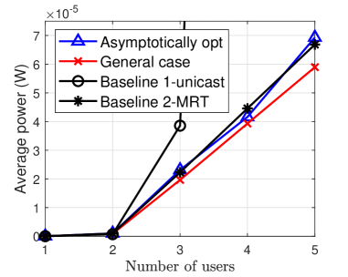
(a) Average power versus $K$. $M=4$, $\mathbf{r}=(2,2,3,3,4)$.

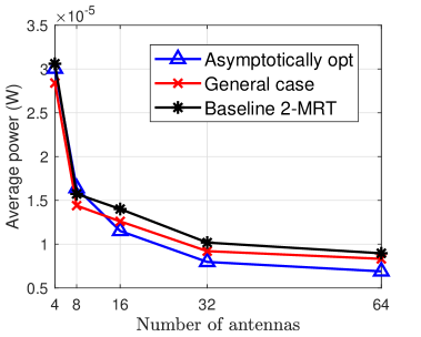
(b) Average power versus $M$. $K=4$, $\mathbf{r}=(2,3,3,4)$.

Figure 2: Average power versus $K$ and $M$.

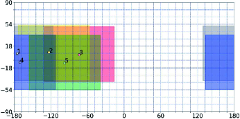
Figure 3: Viewing directions and corresponding FoVs of $5$ users [15].

First, we evaluate the average power over 1,000 random choices for the viewing directions of 1-5 users from 30 users in [15]. Fig. 2 (a) illustrates the average power versus the number of users $K$. We can see that the average powers of the proposed solutions and baseline schemes increase with $K$, as the transmission load increases with $K$. Given the unsatisfactory performance of Baseline 1, we no longer compare with it in the remaining figures. Fig. 2 (b) illustrates the average power versus the number of antennas $M$. We can see the powers achieved by the proposed solutions and baseline schemes decrease with $M$. Besides, by Fig. 2 (b), we can observe that the proposed asymptotically optimal solution achieves better performance than Baseline 2 when the number of antennas is larger than 8.

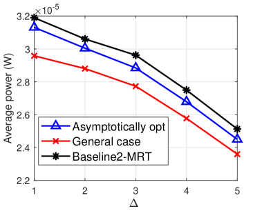
Figure 4: Average power versus $\Delta$. $K=5$, $M=4$, $\mathbf{r}=(2,2,3,3,4)$.

Next, we show the impact of concentration of the viewing directions of all users. We choose the viewing directions of 5 users out of 30 users in [15], i.e., $(\nu_{k},\gamma_{k})_{k\in\{1,\ldots,5\}}$, as shown in Fig. 3. Based on the chosen viewing directions, we consider five sets of viewing directions, i.e., $(\nu_{1}+\Delta,\gamma_{1}),(\nu_{2}+\Delta,\gamma_{2}),(\nu_{3},\gamma_{3}),(\nu_{4}-\Delta,\gamma_{4}),$ and $(\nu_{5}-\Delta,\gamma_{5})$, $\Delta=1,\ldots,5$, and evaluate the corresponding average powers. Note that $\Delta$ reflects the concentration of the viewing directions of the 5 users. In particular, the concentration increases with $\Delta$. Fig. 4 shows the average power versus the concentration parameter $\Delta$. It can be observed that the average power of each multicast scheme decreases with $\Delta$, since multicast opportunities increase with $\Delta$. Finally, from Fig. 2 and Fig. 4, it can be observed that the proposed solutions perform better than the baseline schemes. Specifically, the proposed solutions outperform Baseline 1, as they achieve a higher spectral efficiency utilizing multicast opportunities. The proposed solutions outperform Baseline 2, as they carefully choose beamforming vectors.

V Conclusion

In this paper, we studied optimal transmission of a multi-quality tiled 360 VR video to multiple users in an MIMO-OFDMA system. We minimized the total transmission power by optimizing the beamforming vector and subcarrier, transmission power and rate allocation. This is a challenging mixed discrete-continuous optimization problem. We obtained an asymptotically optimal solution in the case of a large antenna array, and a suboptimal solution in the general case. Finally, numerical results showed that the proposed solutions achieve significant gains over existing schemes.

References

• [1] R. Ju, J. He, F. Sun, J. Li, F. Li, J. Zhu, and L. Han, “Ultra wide view based panoramic VR streaming,” in Proc. of the Workshop on VR/AR Network, Aug. 2017, pp. 19–23.
• [2] C. Guo, Y. Cui, and Z. Liu, “Optimal multicast of tiled 360 VR video,” IEEE Wireless Commun. Lett., vol. 8, no. 1, pp. 145–148, Feb. 2019.
• [3] ——, “Optimal multicast of tiled 360 VR video in OFDMA systems,” IEEE Commun. Lett., vol. 22, no. 12, pp. 2563–2566, Oct. 2018.
• [4] H. Ahmadi, O. Eltobgy, and M. Hefeeda, “Adaptive multicast streaming of virtual reality content to mobile users,” in Proc. of the on Thematic Workshops of ACM Multimedia, Oct. 2017, pp. 170–178.
• [5] N. Kan, C. Liu, J. Zou, C. Li, and H. Xiong, “A server-side optimized hybrid multicast-unicast strategy for multi-user adaptive 360-degree video streaming,” in Proc. of IEEE ICIP, Sep. 2019, pp. 141–145.
• [6] K. Long, C. Ye, Y. Cui, and Z. Liu, “Optimal multi-quality multicast for 360 virtual reality video,” in Proc. of IEEE GLOBECOM, Dec. 2018, pp. 1–6.
• [7] K. Long, Y. Cui, C. Ye and Z. Liu, “Optimal wireless streaming of multi-Quality 360 VR video by exploiting natural, relative smoothness-enabled and transcoding-enabled multicast opportunities,” IEEE Trans. on Multimedia, doi: 10.1109/TMM.2020.3029880.
• [8] J. Xu, S. Lee, W. Kang, and J. Seo, “Adaptive resource allocation for MIMO-OFDM based wireless multicast systems,” IEEE Trans. Broadcast., vol. 56, no. 1, pp. 98–102, Mar. 2010.
• [9] G. Venkatraman, A. Tolli, M. Juntti, and L. Tran, “Multigroup multicast beamformer design for MISO-OFDM with antenna selection,” IEEE Trans. Signal Process., vol. 65, no. 22, pp. 5832–5847, Nov. 2017.
• [10] N. D. Sidiropoulos, T. N. Davidson, and Z.-Q. Luo, “Transmit beamforming for physical-layer multicasting,” IEEE Trans. Signal Process., vol. 54, no. 6, pp. 2239–2251, Jun. 2006.
• [11] C. Guo, L. Zhao, Y. Cui, Z. Liu and D. Ng, “Power-efficient wireless streaming of multi-quality tiled 360 VR video in MIMO-OFDMA systems,” to appear in IEEE Trans. Wireless Commun., 2021.
• [12] Z. Xiang, M. Tao, and X. Wang, “Massive MIMO multicasting in noncooperative cellular networks,” IEEE J. Sel. Areas. Commun., vol. 32, no. 6, pp. 1180–1193, Jun. 2014.
• [13] T. Lipp and S. Boyd, “Variations and extension of the convex–concave procedure,” Optimization and Engineering, vol. 17, no. 2, pp. 263–287, Jun. 2016.
• [14] C. Guo, Y. Cui, D. W. K. Ng, and Z. Liu, “Multi-quality multicast beamforming with scalable video coding,” IEEE Trans. Commun., vol. 66, no. 11, pp. 5662–5677, Nov. 2018.
• [15] “360-degree videos head movements dataset,” http://dash.ipv6.enstb.fr/headMovements/.