Lamperti Semi-Discrete method

Abstract.

We study the numerical approximation of numerous processes, solutions of nonlinear stochastic differential equations, that appear in various applications such as financial mathematics and population dynamics. Between the investigated models are the CIR process, also known as the square root process, the constant elasticity of variance process CEV, the Heston $3/2$-model, the Aït-Sahalia model and the Wright-Fisher model. We propose a version of the semi-discrete method, see [1], which we call Lamperti semi-discrete (LSD) method. The LSD method is domain preserving and seems to converge strongly to the solution process with order $1$ and no extra restrictions on the parameters or the step-size.

1. CIR model

Let

(1) $$x_{t}=x_{0}+\int_{0}^{t}(k_{1}-k_{2}x_{s})ds+\int_{0}^{t}k_{3}\sqrt{x_{s}}dW_{s},\quad t\geq 0.$$

SDE (1) is known as the CIR process, or square root process with a solution remaining in the positive axis, i.e. $x_{t}>0$ a.s. when $(k_{3})^{2}\leq 2k_{1}$ and $x_{0}>0,$ c.f. [2]. The Lamperti transformation of (1) is $z=\frac{2}{k_{3}}\sqrt{x}$ and application of the Itô formula implies the following representation, see Appendix A,

(2) $$z_{t}=z_{0}+\int_{0}^{t}\left(\frac{2k_{1}}{(k_{3})^{2}}(z_{s})^{-1}-\left(\frac{k_{2}}{2}+\frac{(k_{3})^{2}}{8}\right)z_{s}\right)ds+\int_{0}^{t}dW_{s},\,\,t\geq 0.$$

To simplify notation, set $a:=\frac{2k_{1}}{(k_{3})^{2}}$ and $b:=\frac{k_{2}}{2}+\frac{(k_{3})^{2}}{8}.$ The new coefficients $a$ and $b$ are positive. We consider three versions of the semi-discrete method for approximating (2). In the first two versions $(y_{t})$ and $(\hat{y}_{t}),$ see Section 1.1, we use the semi-discrete method as originally proposed, see [3]; we discretize parts of the drift coefficient producing a new differential equation in each subinterval with known solution or a solution that is easily simulated or approximated. In the third version $(\breve{y}_{t})$ we examine a new modification of the semi-discrete method, where in each subinterval $(t_{n},t_{n+1}]$ we do not need to solve a new differential equation, but only an algebraic equation.

1.1. Lamperti Semi-Discrete methods $\widetilde{z}^{1}_{n}$ and $\widetilde{z}^{2}_{n}$ for CIR

Rewrite (2) as

(3) $$z_{t}=z_{0}+\int_{0}^{t}\left(a(z_{s})^{-1}-bz_{s}\right)ds+\int_{0}^{t}dW_{s},\,\,t\geq 0.$$

To approximate the constant diffusion SDE (3) we use the following two versions of the semi-discrete method. In the first version $(y_{t})$, we discretize the linear part of the drift coefficient and in the second $(\hat{y}_{t})$ we leave it as it since it produces a differential equation with known solution. Let $t\in(t_{n},t_{n+1}],$ where we assume the length of each subinterval to be equal to $\Delta$ and consider

(4) $$y_{t}=\Delta W_{n}+y_{t_{n}}-by_{t_{n}}\Delta+\int_{t_{n}}^{t}a(y_{s})^{-1}ds,$$

with $y_{0}=z_{0}$ and

(5) $$\hat{y}_{t}=\Delta W_{n}+\hat{y}_{t_{n}}+\int_{t_{n}}^{t}\left(a(\hat{y}_{s})^{-1}-b\hat{y}_{s}\right)ds,$$

with $\hat{y}_{0}=z_{0}$

(4) and (5) are Bernoulli type equations with solutions satisfying, see Appendix B,

(6) $$(y_{t})^{2}=\left(\Delta W_{n}+(1-b\Delta)y_{t_{n}}\right)^{2}+2a(t-t_{n})$$

and

(7) $$(\hat{y}_{t})^{2}=(\Delta W_{n}+\hat{y}_{t_{n}})^{2}e^{-2b(t-t_{n})}+a\frac{1-e^{-2b(t-t_{n})}}{b},$$

respectively.

We propose the following versions of the semi-discrete method for the approximation of (2),

(8) $$y_{t_{n+1}}=\sqrt{\left(\Delta W_{n}+(1-b\Delta)y_{t_{n}}\right)^{2}+2a\Delta}$$

and

(9) $$\hat{y}_{t_{n+1}}=\sqrt{(\Delta W_{n}+\hat{y}_{t_{n}})^{2}e^{-2b\Delta}+a\frac{1-e^{-2b\Delta}}{b}},$$

which suggests the versions of the Lamperti semi-discrete method $(\widetilde{z}^{1}_{n})_{n\in{\mathbb{N}}},(\widetilde{z}^{2}_{n})_{n\in{\mathbb{N}}}$ for the approximation of (1)

(10) $$\widetilde{z}^{1}_{t_{n+1}}=\frac{(k_{3})^{2}}{4}\left(\left(\Delta W_{n}+(1-b\Delta)y_{t_{n}}\right)^{2}+2a\Delta\right)$$

and

(11) $$\widetilde{z}^{2}_{t_{n+1}}=\frac{(k_{3})^{2}}{4}\left((\Delta W_{n}+\hat{y}_{t_{n}})^{2}e^{-2b\Delta}+a\frac{1-e^{-2b\Delta}}{b}\right).$$

1.2. Lamperti Semi-Discrete method $\widetilde{z}^{3}_{n}$ for CIR

In this version of the semi-discrete method, $(\breve{y}_{t})$ we examine a new modification of the semi-discrete method, where in each subinterval $(t_{n},t_{n+1}]$ we do not need to solve a new differential equation, but only an algebraic equation. For $t\in(t_{n},t_{n+1}]$ consider

(12) $$\breve{y}_{t}=W_{t}-W_{t_{n}}+\breve{y}_{t_{n}}+a(\breve{y}_{t})^{-1}\Delta-b\breve{y}_{t}\Delta.$$

with $\breve{y}_{0}=z_{0}.$ The solution of (12) satisfies

(13) $$(1+b\Delta)(\breve{y}_{t})^{2}-(W_{t}-W_{t_{n}}+\breve{y}_{t_{n}})\breve{y}_{t}-a\Delta=0.$$

We propose the following version of the semi-discrete method for the approximation of (2),

(14) $$\breve{y}_{t_{n+1}}=\frac{\Delta W_{n}+\breve{y}_{t_{n}}+\sqrt{(\Delta W_{n}+\breve{y}_{t_{n}})^{2}+4(1+b\Delta)a\Delta}}{2(1+b\Delta)},$$

which suggests the version of the Lamperti semi-discrete method $(\widetilde{z}^{3}_{n})_{n\in{\mathbb{N}}}$ for the approximation of (1)

(15) $$\widetilde{z}^{3}_{t_{n+1}}=\frac{(k_{3})^{2}}{4}\left(\frac{\Delta W_{n}+\breve{y}_{t_{n}}+\sqrt{(\Delta W_{n}+\breve{y}_{t_{n}})^{2}+4(1+b\Delta)a\Delta}}{2(1+b\Delta)}\right)^{2}.$$

1.3. Numerical experiment for CIR

For a minimal numerical experiment we present simulation paths for the numerical approximation of (1) with $x_{0}=4$ and compare with the SD method proposed in [4], which reads

(16) $$\widetilde{y}_{t_{n+1}}=\left(\sqrt{\widetilde{y}_{t_{n}}(1-\frac{k_{2}\Delta}{1+k_{2}\theta\Delta})+\frac{\Delta}{1+k_{2}\theta\Delta}\left(k_{1}-\frac{(k_{3})^{2}}{4(1+k_{2}\theta\Delta)}\right)}+\frac{k_{3}}{2(1+k_{2}\theta\Delta)}\Delta W_{n}\right)^{2},$$

where $\theta$ represents the level of implicitness. The case $\theta=0$ was studied in [3] where the idea of the semi-discrete method was originally presented. According to the results in [4] it is shown that SD method (16) is strongly convergent under some conditions on the coefficients $k_{i},$ the level of implicitness $\theta$ and the step-size $\Delta.$ In particular, it strongly converges to the solution of (1) with a logarithmic rate if also ${\mathbb{E}}(x_{0})^{p}<A$ for some $p\geq 2,(k_{3})^{2}\leq 4k_{1}(1+k_{2}\theta\Delta)$ and $\Delta(1-\theta)\leq(k_{2})^{-1},$ while a polynomial rate of convergence is achieved with order at least $1/4$ for a smaller set of parameters, namely $(k_{3})^{2}\leq 2k_{1}$ and $(\frac{2k_{1}}{(k_{3})^{2}}-1)^{2}>16$ for $\theta=0,$ with $x_{0}\in{\mathbb{R}}.$ On the other hand, the LSD scheme (10) seems to work without any restriction on the step-size or on the parameters which is a very interesting result.

Remark 1.

We would like to point out a mistake that escaped our attention. In the proof of the strong convergence properties of the SD scheme (16) proposed in [4] an auxiliary process $(h_{t})$ appears, see [4, Rel. (2.3)]

$$h_{t}=x_{0}+\int_{0}^{t}(\underbrace{k_{1}-k_{2}(1-\theta)y_{\hat{s}}-k_{2}\theta y_{\tilde{s}}}_{f_{\theta}(y_{\hat{s}},y_{\tilde{s}})})ds+\int_{0}^{t}k_{3}\sqrt{y_{s}}dW_{s},$$

where $\hat{s}=t_{j}$ when $s\in(t_{j},t_{j+1}],j=0,1,\ldots,n$ and

$$\widetilde{s}=\left\{\begin{array}[]{ll}t_{j+1},&\mbox{for }\,s\in[t_{j},t_{j+1}],\\ t,&\mbox{for }\,s\in[t_{n},t]\end{array}j=0,\ldots,n-1.\right.$$

The problem is that we can not apply directly the Itô formula on $(h_{t})$ since $y_{\tilde{s}}$ is ${\mathcal{F}}_{t_{n+1}}$-measurable and not ${\mathcal{F}}_{t_{n}}$-measurable. Nevertheless, writing the drift of $(h_{t})$ as $f_{\theta}(y_{\hat{s}},y_{\hat{s}})$ we can proceed in the same way. The remainder term $f_{\theta}(y_{\hat{s}},y_{\tilde{s}})-f_{\theta}(y_{\hat{s}},y_{\hat{s}})=k_{2}\theta(y_{\hat{s}}-y_{\tilde{s}})$ can be easily bounded.

We also present the implicit scheme proposed in [5], which takes the following form

(17) $$\bar{y}_{t_{n+1}}=\left(\frac{\sqrt{4(\bar{y}_{t_{n}}+(k_{1}-\frac{(k_{3})^{2}}{2})\Delta)(1+k_{2}\Delta)+(k_{3})^{2}(\Delta W_{n})^{2}}+k_{3}\Delta W_{n}}{2(1+k_{2}\Delta)}\right)^{2},$$

As a first graphical illustration we borrow the set of parameters from [4, Sec.4]; we take $k_{1}=k_{2}=2,k_{3}=1,T=1$ and $\theta=1$ with various step-sizes $\Delta=10^{-4}$ and $\Delta=10^{-3},\Delta=10^{-2}.$ We compare with the proposed two versions of LSD scheme (10) and (11) and the implicit method ALF (17). Figure 1 shows that all the schemes perform in a similar way. We also give a presentation of the difference of the various SD approximations in Figure 2.

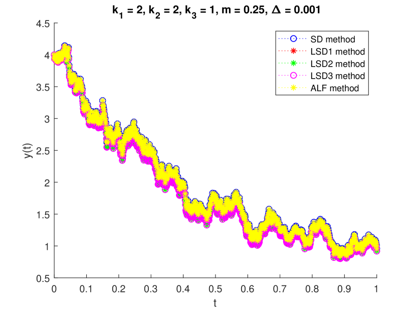
(a) Trajectories of (10)-(17).

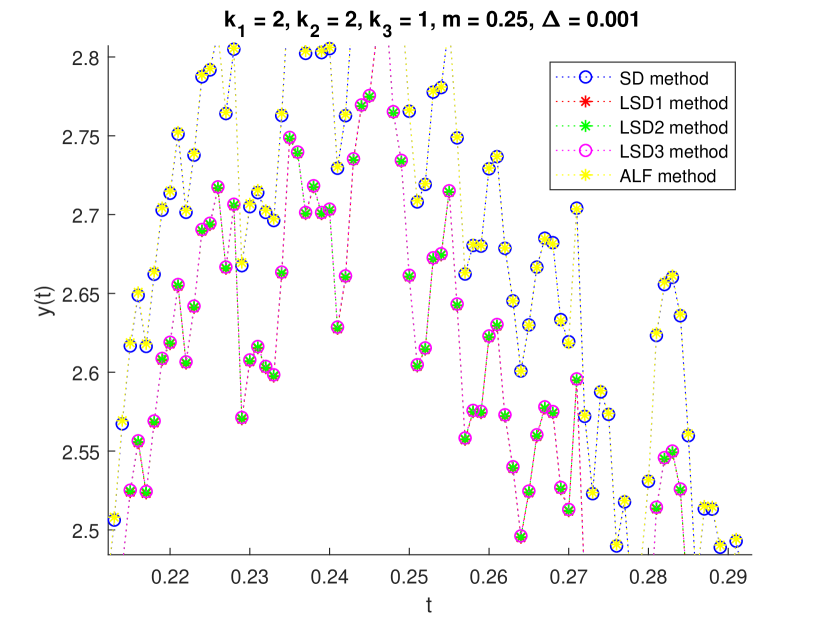
(b) Zoom of Figure 1(A).

Figure 1. Trajectories of (10), (11), (15), (16) and (17) for the approximation of (1) with $\Delta=10^{-4}$.

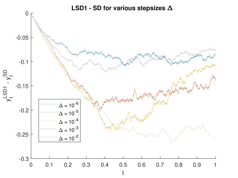
(a) Difference (10) - (16) for various step sizes.

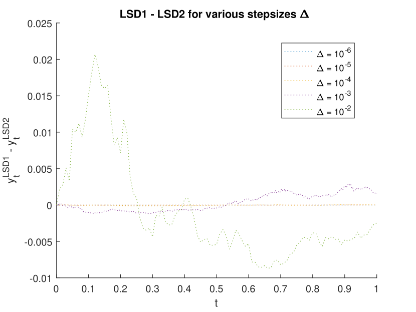
(b) Difference (10) - (11) for various step sizes.

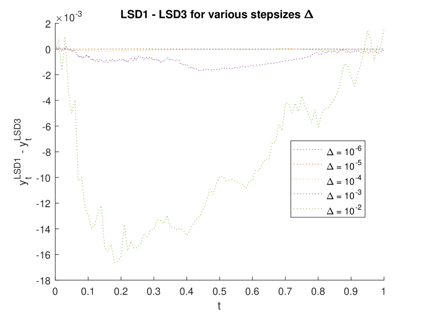
(c) Difference (10) - (15) for various step sizes.

Figure 2. Trajectories of the differences of the semi-discrete methods (10), (11) and (16) for the approximation of (1) with various step-sizes.

For a different configuration, we are able to compare with the exact solution. Note that by choosing $d=4k_{1}/(k_{3})^{2}=2$ then the solution of (1) is $x_{t}=(x_{1}(t))^{2}+(x_{2}(t))^{2},$ where $x_{j}(t)$ is the solution of the Orstein-Uhlenbelck process

(18) $$dx_{j}(t)=-\frac{1}{2}k_{2}x_{j}(t)dt+\frac{1}{2}k_{3}dW^{(j)}_{t}$$

and the Brownian motions $W^{(j)}_{t}$ are independent. For $t\in[t_{n},t_{n+1}]$ the solution of (18) is

(19) $$x_{j}(t)=e^{-\frac{1}{2}k_{2}(t-t_{n})}x_{j}(t_{n})+\frac{1}{2}k_{3}e^{-\frac{1}{2}k_{2}(t-t_{n})}\int_{t_{n}}^{t}e^{\frac{1}{2}k_{2}(s-t_{n})}dW^{(j)}_{s}.$$

Actually, we approximate in each subinterval $[t_{n},t_{n+1}]$ the last stochastic integral in (19) at $t_{n}$ producing the sequence

(20) $$x_{j}(t_{n+1})=e^{-\frac{1}{2}k_{2}\Delta}x_{j}(t_{n})+\frac{k_{3}}{k_{2}}(1-e^{-\frac{1}{2}k_{2}\Delta})\Delta W^{(j)}_{n}$$

and therefore the solution process of (1) at the grid points reads

(21) $$x(t_{n+1}) = \left(e^{-\frac{1}{2}k_{2}\Delta}x_{1}(t_{n})+\frac{k_{3}}{k_{2}}(1-e^{-\frac{1}{2}k_{2}\Delta})\Delta W^{(1)}_{n}\right)^{2}$$

$$+\left(e^{-\frac{1}{2}k_{2}\Delta}x_{2}(t_{n})+\frac{k_{3}}{k_{2}}(1-e^{-\frac{1}{2}k_{2}\Delta})\Delta W^{(2)}_{n}\right)^{2}.$$

We therefore choose $k_{3}=2$ for this second experiment, with all the other parameters unchanged, so that $d=2.$ Moreover $x(0)=(x_{1}(0))^{2}+(x_{2}(0))^{2}.$ We present in Figure 3 simulation paths of (10)-(17) and the exact solution (20) choosing as initial conditions $x_{1}(0)=\sqrt{mx(0)},x_{2}(0)=\sqrt{(1-m)x(0)}$ for different $0<m<1.$ Moreover, the driving Wiener process in this case is produced in the following way

(22) $$W(t)=\int_{0}^{t}\frac{x_{1}(u)dW^{(1)}_{u}+x_{2}(u)dW^{(2)}_{u}}{\sqrt{x(u)}}.$$

In practice the increments of the Wiener process we use for the derivation of the paths of all the approximation methods are

(23) $$\Delta W_{n}=\frac{x_{1}(t_{n})\Delta W^{(1)}_{n}+x_{2}(t_{n})\Delta W^{(2)}_{n}}{\sqrt{x(t_{n})}}.$$

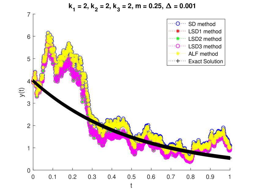
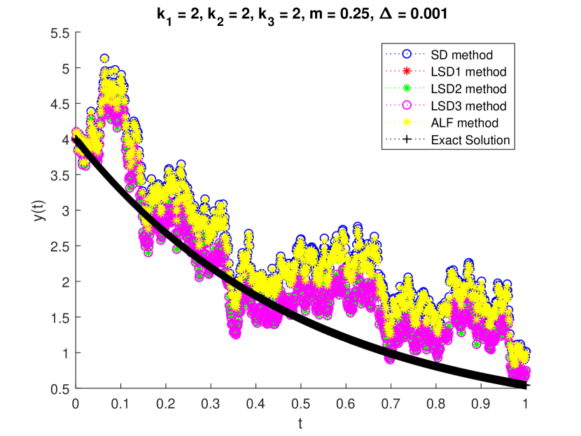
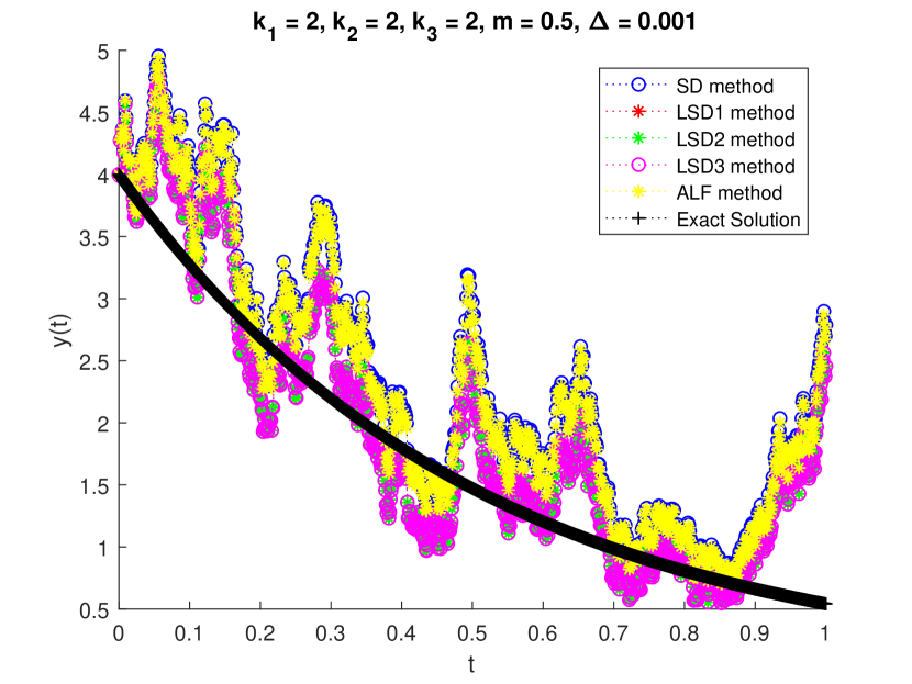
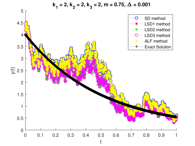
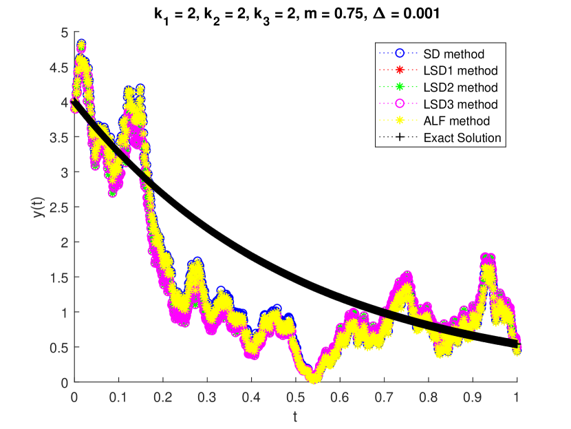
Figure 3. Trajectories of (10)-(17) and the exact solution (21) with different $m$ and $\Delta=0.001.$

In Figure 3 we cannot see the differences between the methods. By considering bigger step-sizes $\Delta,$ we take the picture in Figure 4 where again we see the relation between the schemes.

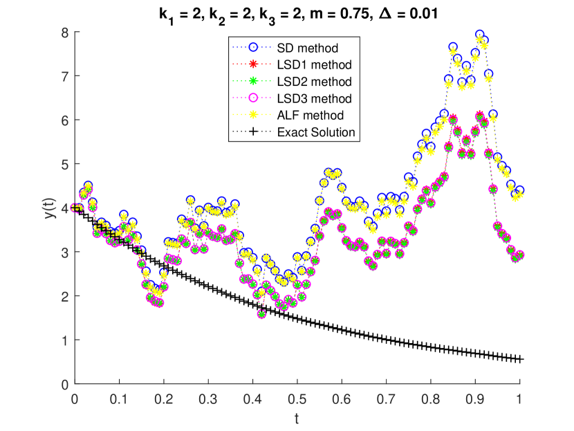
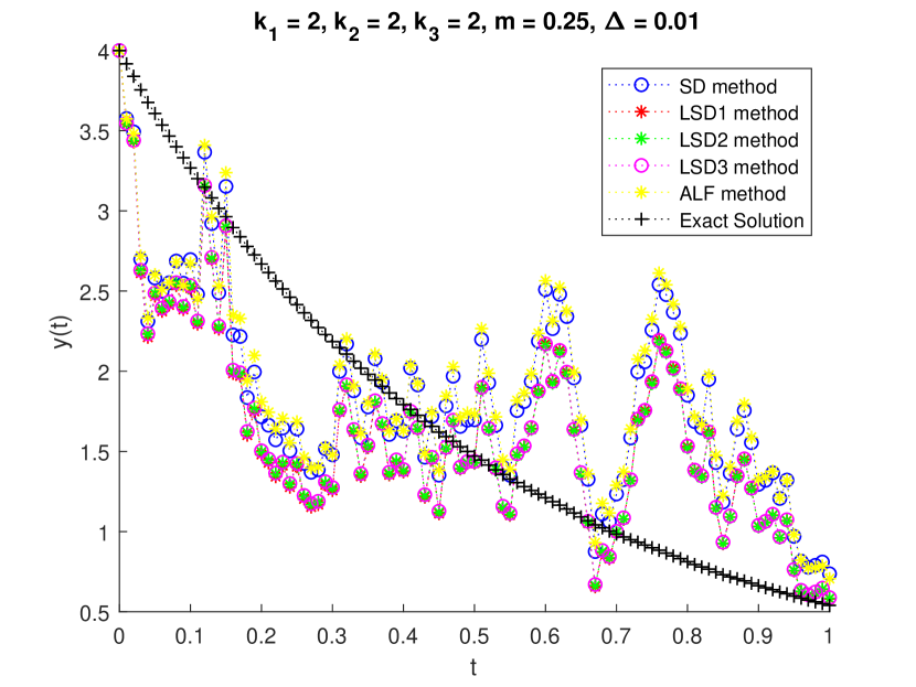
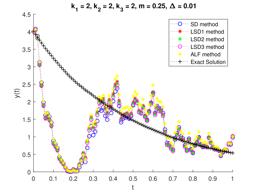
Figure 4. Trajectories of (10)-(17) and the exact solution (21) with different $m$ and $\Delta.$

We note that the exact solution has a very similar behavior between different realizations of the Wiener processes. We need to take a bigger $\Delta=0.1$ to notice a small variation of the produced solution, see Figure 5.

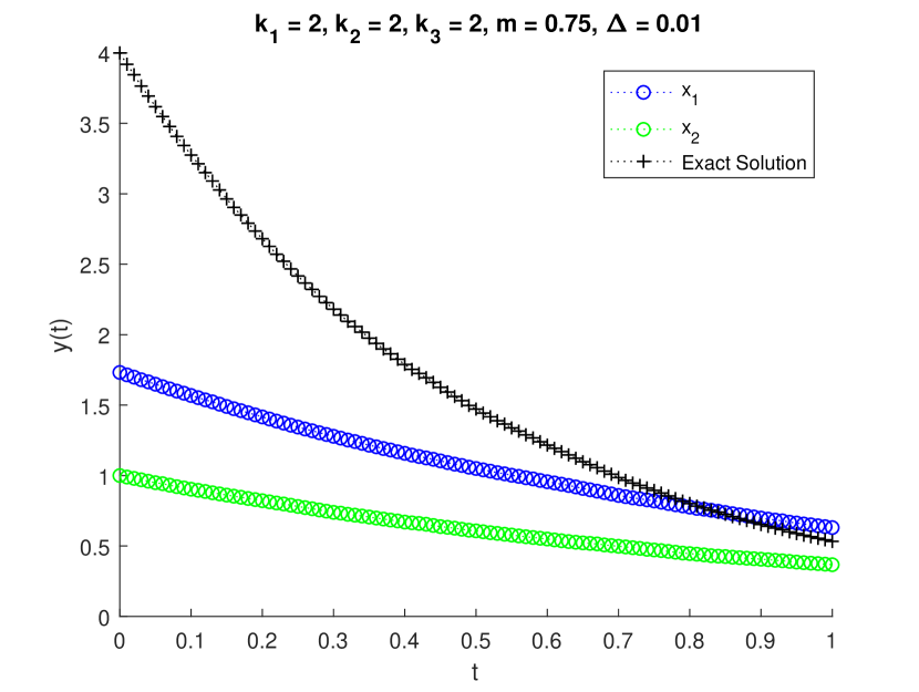
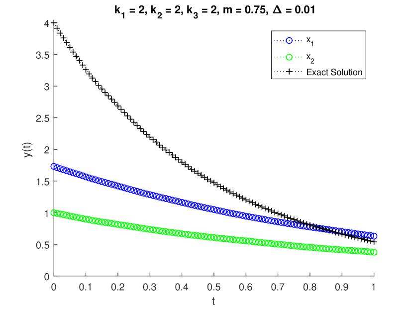
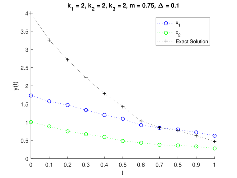
Figure 5. Trajectories of the processes $x_{1}$ and $x_{2}$ which give the exact solution (21) with different step-sizes $\Delta.$

We also examine numerically the order of strong convergence of the LSD method. The numerical results suggest that the Lamperti Semi-Discrete methods converge in the mean-square sense with order close to $1,$ see Figure 6.

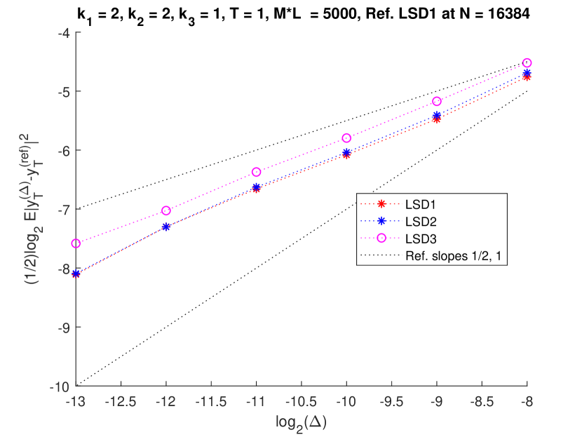
(a) LSD1 as reference solution.

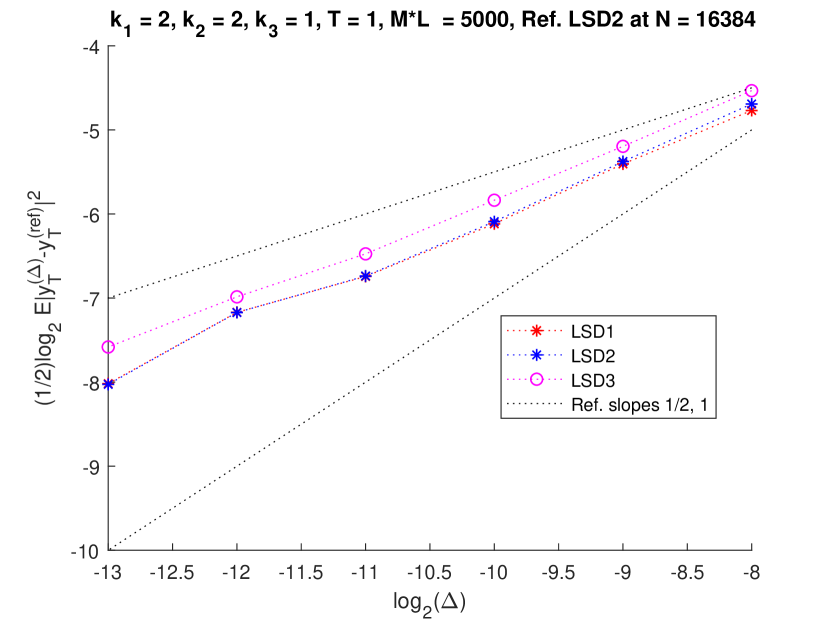
(b) LSD2 as reference solution.

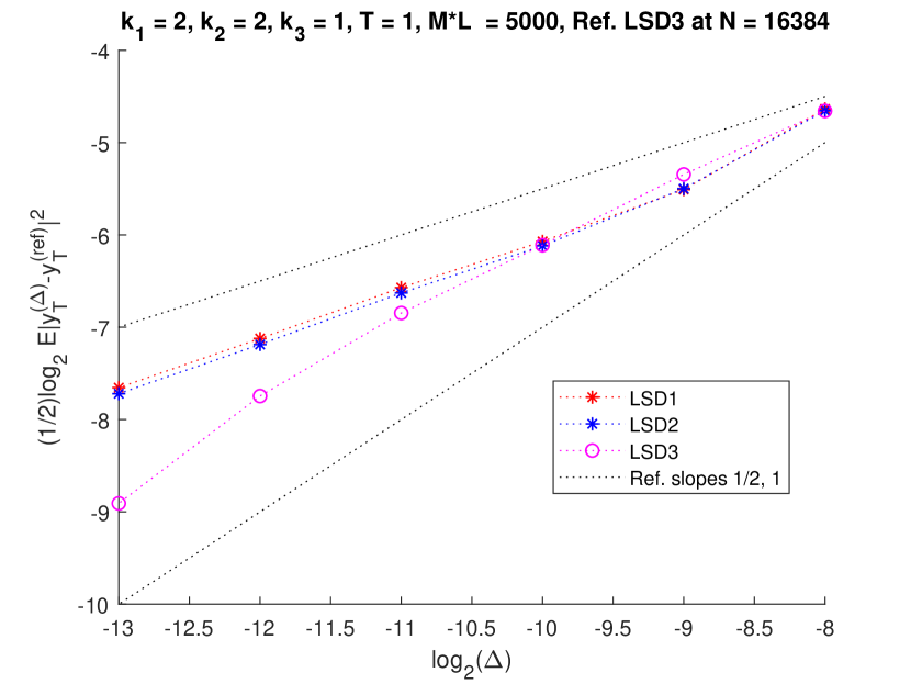
(c) LSD3 as reference solution.

Figure 6. Convergence of Lamperti Semi-Discrete methods (10), (11) and (15) for the approximation of (1) with different reference solution.

Moreover, we perform one more numerical experiment to show the ability of the method to produce nonnegative solutions, outside the usual restrictions on the parameters, $(k_{3})^{2}\leq 2k_{1}.$ The solution of the CIR process is nonnegative, with no extra restriction on the positive parameters $k_{i},i=1,2,3,$ i.e. $x_{t}\geq 0$ a.s. when $x_{0}>0.$ Therefore, we change a bit the parameters, taking $k_{1}=1,k_{2}=2$ and different values for $k_{3}$ so that $(k_{3})^{2}>2k_{1}.$ In this case the proposed LSD methods (10), (11) and (15) work in the sense that they produce nonnegative values, whereas the implicit method (17) as well as the implicit method proposed in [6], which also takes an explicit representation in this case,

(24) $$\check{y}_{t_{n+1}}=\left(\frac{\sqrt{(\check{y}_{t_{n}}+\frac{1}{2}k_{3}\Delta W_{n})^{2}+(k_{1}-\frac{(k_{3})^{2}}{4})\Delta}+\check{y}_{t_{n}}+\frac{1}{2}k_{3}\Delta W_{n}}{2+k_{2}\Delta}\right)^{2},$$

with $\check{y}_{0}=\sqrt{x_{0}},$ do not even produce real values, see Figure 7 where for (17) and (24) the real parts of the solution is presented. Note that as $k_{3}$ increases the implicit methods (17) and (24) show an erratic behavior.

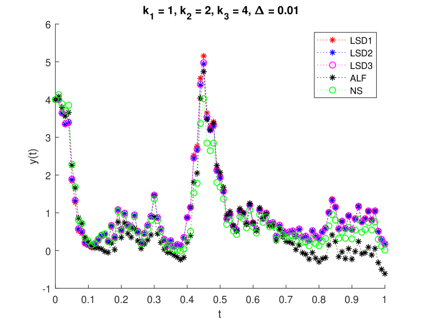
(a) $k_{3}=4,\Delta=10^{-2}.$

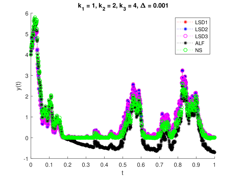
(b) $k_{3}=4,\Delta=10^{-3}.$

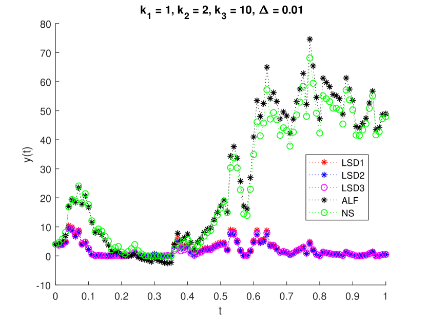
(c) $k_{3}=10,\Delta=10^{-2}.$

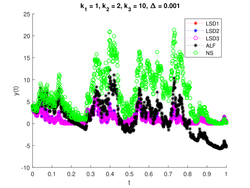
(d) $k_{3}=10,\Delta=10^{-3}.$

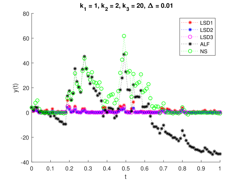
(e) $k_{3}=20,\Delta=10^{-2}.$

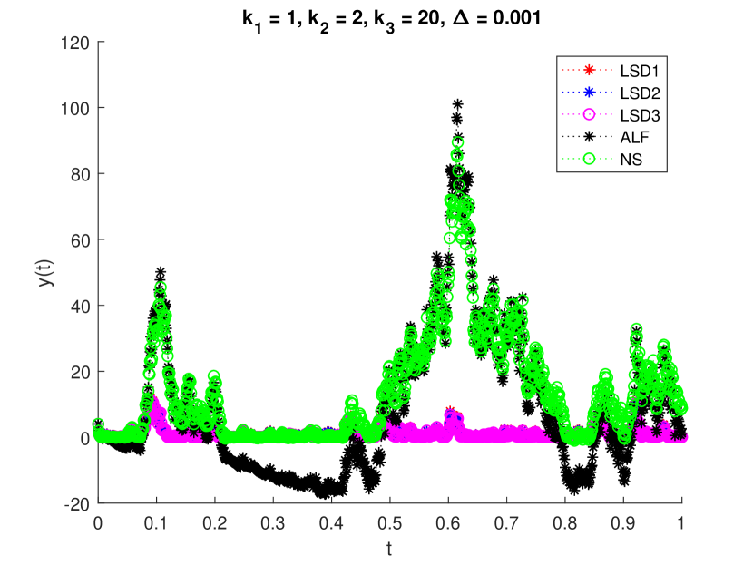
(f) $k_{3}=20,\Delta=10^{-3}.$

Figure 7. Trajectories of (10), (11), (15), (17) and (24) for the approximation of (1) with different coefficients and various $\Delta.$

Finally, we present numerically the order of strong convergence of the LSD methods, see Figure 8, where we can once more see that it is close to $1.$

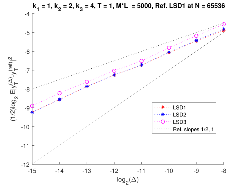
(a) LSD1 as reference solution.

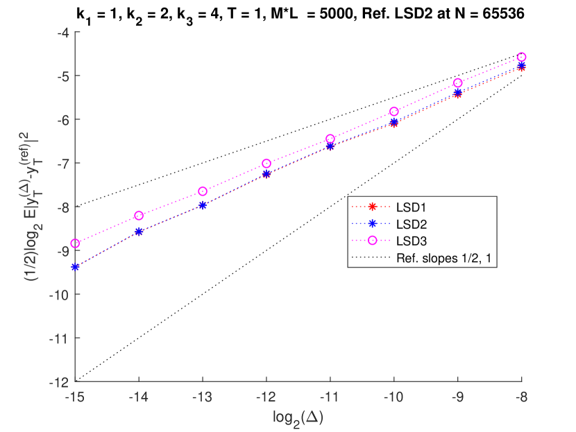
(b) LSD2 as reference solution.

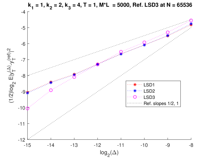
(c) LSD3 as reference solution.

Figure 8. Convergence of Lamperti Semi-Discrete methods (10), (11) and (15) for the approximation of (1) with different reference solution.

2. CEV model

Let

(25) $$x_{t}=x_{0}+\int_{0}^{t}(k_{1}-k_{2}x_{s})ds+\int_{0}^{t}k_{3}(x_{s})^{q}dW_{s},\quad t\geq 0.$$

where $k_{1},k_{2},k_{3}$ are positive and $1/2<q<1.$ SDE (25) is a mean-reverting constant elasticity of variance process (CEV) with $x_{t}>0$ a.s. c.f. [7, App. A]. The Lamperti transformation of (25) is $z=\frac{1}{k_{3}(1-q)}x^{1-q}$ with dynamics,

(26) $$z_{t}=z_{0}+\int_{0}^{t}\left(k_{1}k_{3}^{\frac{1-2q}{1-q}}(1-q)^{\frac{-q}{1-q}}(z_{s})^{-\frac{q}{1-q}}-\frac{q}{2(1-q)}(z_{s})^{-1}-k_{2}(1-q)z_{s}\right)ds+\int_{0}^{t}dW_{s}.$$

Set $a=k_{1}k_{3}^{\frac{1-2q}{1-q}}(1-q)^{\frac{-q}{1-q}},b=q/(2-2q)$ and $c=k_{2}(1-q).$ We consider two versions of the semi-discrete method for approximating (26). In the first version $(y_{t}),$ see Section 2.1, we use the semi-discrete method as originally proposed, and in the second version we examine the new version $(\hat{y}_{t}),$ see Section 2.2, where in each subinterval $(t_{n},t_{n+1}]$ we solve an algebraic equation.

2.1. Lamperti Semi-Discrete method $\widetilde{z}^{1}_{n}$ for CEV

Rewrite (26) as

(27) $$z_{t}=z_{0}+\int_{0}^{t}\left(a(z_{s})^{-\frac{q}{1-q}}-b(z_{s})^{-1}-cz_{s}\right)ds+\int_{0}^{t}dW_{s}.$$

where $a,b,c$ positive. We consider the following semi-discrete method for approximating (26),

(28) $$y_{t} = \Delta W_{n}+y_{t_{n}}+\int_{t_{n}}^{t}\left(\frac{a}{(y_{t_{n}})^{\frac{2q-1}{1-q}}}(y_{s})^{-1}-\frac{b}{(y_{t_{n}})^{2}}y_{t}-cy_{s}\right)ds$$

$$= \phi_{\Delta}(y_{t_{n}},\Delta W_{n})+\int_{t_{n}}^{t}\left(B_{n}(y_{s})^{-1}+C_{n}y_{s}\right)ds$$

with $y_{0}=z_{0},$ where $\phi_{\Delta}(x,y)=\frac{x+y}{1+\frac{b}{x^{2}}\Delta}$ and

$$B_{n}:=\frac{a}{(y_{t_{n}})^{\frac{2q-1}{1-q}}+b(y_{t_{n}})^{\frac{4q-3}{1-q}}\Delta},\,\,C_{n}:=-\frac{c}{1+\frac{b\Delta}{(y_{t_{n}})^{2}}}.$$

The Bernoulli equation (28) has a solution satisfying, see Appendix B,

(29) $$(y_{t})^{2} = \phi^{2}_{\Delta}(y_{t_{n}},\Delta W_{n})\exp\left\{-\frac{2c}{1+\frac{b\Delta}{(y_{t_{n}})^{2}}}(t-t_{n})\right\}$$

$$+\frac{a}{c(y_{t_{n}})^{\frac{2q-1}{1-q}}}\left(1-\exp\left\{-\frac{2c}{1+\frac{b\Delta}{(y_{t_{n}})^{2}}}(t-t_{n})\right\}\right).$$

We propose the following version of the semi-discrete method for the approximation of (26),

(30) $$y_{t_{n+1}}=\sqrt{\phi^{2}_{\Delta}(y_{t_{n}},\Delta W_{n})e^{-\frac{2c}{1+\frac{b\Delta}{(y_{t_{n}})^{2}}}\Delta}+\frac{a}{c(y_{t_{n}})^{\frac{2q-1}{1-q}}}(1-e^{-\frac{2c}{1+\frac{b\Delta}{(y_{t_{n}})^{2}}}\Delta})},$$

which suggests the versions of the Lamperti semi-discrete method $(\widetilde{z}^{1}_{n})_{n\in{\mathbb{N}}},$ for the approximation of (25) with $\widetilde{z}^{1}_{n}=(k_{3}(1-q)y_{n})^{1/(1-q)}$ or

$$\widetilde{z}^{1}_{t_{n+1}}=(k_{3}(1-q))^{\frac{1}{1-q}}$$

$$\times \left|\phi^{2}_{\Delta}(y_{t_{n}},\Delta W_{n})e^{-\frac{2c\Delta}{1+\frac{b\Delta}{(y_{t_{n}})^{2}}}}+\frac{a}{c(y_{t_{n}})^{\frac{2q-1}{1-q}}}(1-e^{-\frac{2c\Delta}{1+\frac{b\Delta}{(y_{t_{n}})^{2}}}})\right|^{1/(2-2q)}.$$

2.2. Lamperti Semi-Discrete methods $\widetilde{z}^{2}_{n},\widetilde{z}^{3}_{n}$ for CEV

Let $t\in(t_{n},t_{n+1}]$ and consider the processes $(\hat{y}_{t})$ and $(\widetilde{y}_{t})$ where

(32) $$\hat{y}_{t}=W_{t}-W_{t_{n}}+\hat{y}_{t_{n}}+a(\hat{y}_{t_{n}})^{\frac{1-2q}{1-q}}(\hat{y}_{t})^{-1}\Delta-b(\hat{y}_{t_{n}})^{-1}\Delta-c\hat{y}_{t}\Delta,$$

with $\hat{y}_{0}=z_{0}$ and

(33) $$\widetilde{y}_{t}=W_{t}-W_{t_{n}}+\widetilde{y}_{t_{n}}+a(\widetilde{y}_{t_{n}})^{\frac{-q}{1-q}}\Delta-b(\widetilde{y}_{t_{n}})^{-1}\Delta-(\widetilde{y}_{t_{n}})^{-1}\Delta+(\widetilde{y}_{t})^{-1}\Delta-c\widetilde{y}_{t}\Delta,$$

with $\widetilde{y}_{0}=z_{0}.$

The solution of (32) is such that

(34) $$(1+c\Delta)(\hat{y}_{t})^{2}-\left(W_{t}-W_{t_{n}}+\hat{y}_{t_{n}}-b(\hat{y}_{t_{n}})^{-1}\Delta\right)\hat{y}_{t}-a(\hat{y}_{t_{n}})^{\frac{1-2q}{1-q}}\Delta=0,$$

while the solution of (33) satisfies

(35) $$(1+c\Delta)(\widetilde{y}_{t})^{2}-\left(W_{t}-W_{t_{n}}+\widetilde{y}_{t_{n}}+(a(\widetilde{y}_{t_{n}})^{\frac{-q}{1-q}}-b(\widetilde{y}_{t_{n}})^{-1})\Delta\right)\widetilde{y}_{t}-\Delta=0$$

We propose the following versions of the semi-discrete method for the approximation of (26),

(36) $$\hat{y}_{t_{n+1}}=\frac{\hat{\phi}_{\Delta}(\hat{y}_{t_{n}},\Delta W_{n})+\sqrt{\hat{\phi}^{2}_{\Delta}(\hat{y}_{t_{n}},\Delta W_{n})+4a\Delta(1+c\Delta)(\hat{y}_{t_{n}})^{\frac{1-2q}{1-q}}}}{2(1+c\Delta)},$$

with $\hat{\phi}_{\Delta}(x,y)=(y+x-bx^{-1}\Delta),$ and

(37) $$\widetilde{y}_{t_{n+1}}=\frac{\widetilde{\phi}_{\Delta}(\widetilde{y}_{t_{n}},\Delta W_{n})+\sqrt{\widetilde{\phi}^{2}_{\Delta}(\widetilde{y}_{t_{n}},\Delta W_{n})+4\Delta(1+c\Delta)}}{2(1+c\Delta)},$$

with $\widetilde{\phi}_{\Delta}(x,y)=(y+x+ax^{\frac{-q}{1-q}}\Delta-bx^{-1}\Delta),$ which suggest the versions of the Lamperti semi-discrete method $(\widetilde{z}^{2}_{n})_{n\in{\mathbb{N}}},(\widetilde{z}^{3}_{n})_{n\in{\mathbb{N}}}$ for the approximation of (25) with

$$\widetilde{z}^{2}_{t_{n+1}}=(k_{3}(1-q))^{\frac{1}{1-q}}$$

$$\times \left|\frac{\hat{\phi}_{\Delta}(\hat{y}_{t_{n}},\Delta W_{n})+\sqrt{\hat{\phi}^{2}_{\Delta}(\hat{y}_{t_{n}},\Delta W_{n})+4a\Delta(1+c\Delta)(\hat{y}_{t_{n}})^{\frac{1-2q}{1-q}}}}{2(1+c\Delta)}\right|^{1/(1-q)},$$

and

$$\widetilde{z}^{3}_{t_{n+1}}=(k_{3}(1-q))^{\frac{1}{1-q}}$$

$$\times \left|\frac{\widetilde{\phi}_{\Delta}(\widetilde{y}_{t_{n}},\Delta W_{n})+\sqrt{\widetilde{\phi}^{2}_{\Delta}(\widetilde{y}_{t_{n}},\Delta W_{n})+4\Delta(1+c\Delta)}}{2(1+c\Delta)}\right|^{1/(1-q)}.$$

2.3. Numerical experiment for CEV

For a minimal numerical experiment we present simulation paths for the numerical approximation of (25) with $x_{0}=1/16$ and compare with the SD method proposed in [7], which reads

(40) $$\widetilde{y}_{t_{n+1}} = \Big{(}\sqrt{\widetilde{y}_{t_{n}}\left(1-\frac{k_{2}\Delta}{1+k_{2}\theta\Delta}\right)+\frac{k_{1}\Delta}{1+k_{2}\theta\Delta}-\frac{(k_{3})^{2}\Delta}{4(1+k_{2}\theta\Delta)^{2}}(\widetilde{y}_{t_{n}})^{2q-1}}$$

$$+\frac{k_{3}}{2(1+k_{2}\theta\Delta)}(\widetilde{y}_{t_{n}})^{q-\frac{1}{2}}\Delta W_{n}\Big{)}^{2},$$

where $\theta$ represents the level of implicitness. In particular we choose the coefficients as in [7, Sec.6]; we take $k_{1}=\frac{1}{16},k_{2}=1$ and $k_{3}=0.4$ and $q=3/4$ for the fully implicit SD scheme (40) with $\theta=1$ and compare with the proposed versions of LSD scheme (2.1) and (2.2).

Remark 2.

As in Remark 1, we note that in the proof of the strong convergence properties of the SD scheme (40) proposed in [7] an auxiliary process $(h_{t})$ appears, see [7, Rel. (33)]. Following the same lines the results in [7] as well as in [8] where a more general CIR/CEV-type model is examined with delay, are true.

Moreover, we compare with the implicit method, see [6]. Set

$$G(x)=x-(1-q)\left(k_{1}x^{-q/(1-q)}-k_{2}x-q(k_{3})^{2}x^{-1}/2\right)\Delta$$

and compute

$$y_{n+1}=G^{-1}(y_{n}+k_{3}(1-q)\Delta W_{n})$$

and then transform back to get the following scheme

(41) $$y_{n+1}^{Impl}=(y_{n+1})^{1/(1-q)}.$$

The simulation paths are presented in Figures 9 and 10.

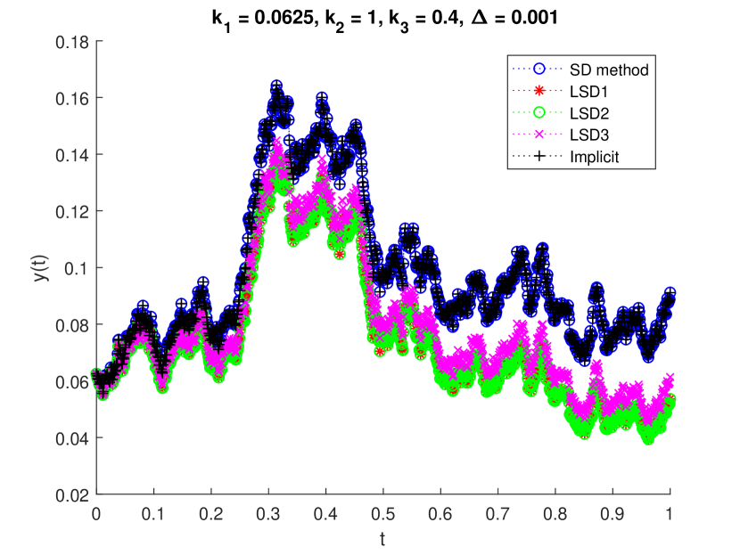
(a) Trajectories with $\Delta=10^{-3}$.

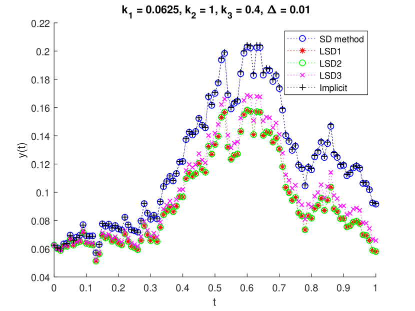
(b) Trajectories with $\Delta=10^{-2}$.

Figure 9. Trajectories of (2.1), (2.2), (2.2), (40) and (41) for the approximation of (25) for different step-sizes.

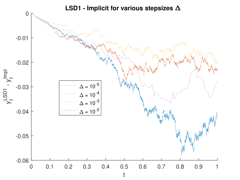
(a) LSD1 - Implicit

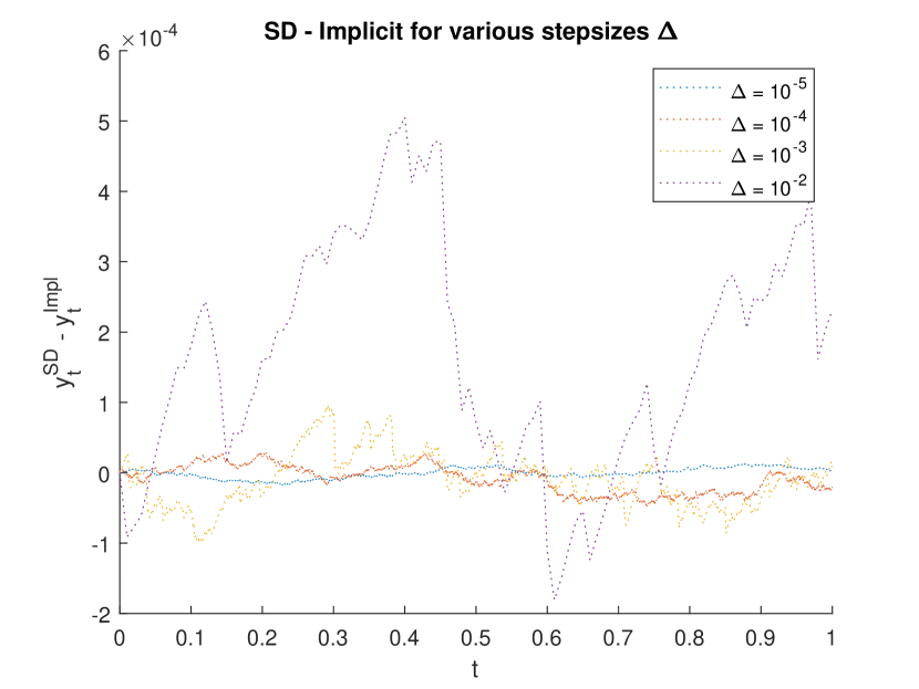
(b) SD - Implicit

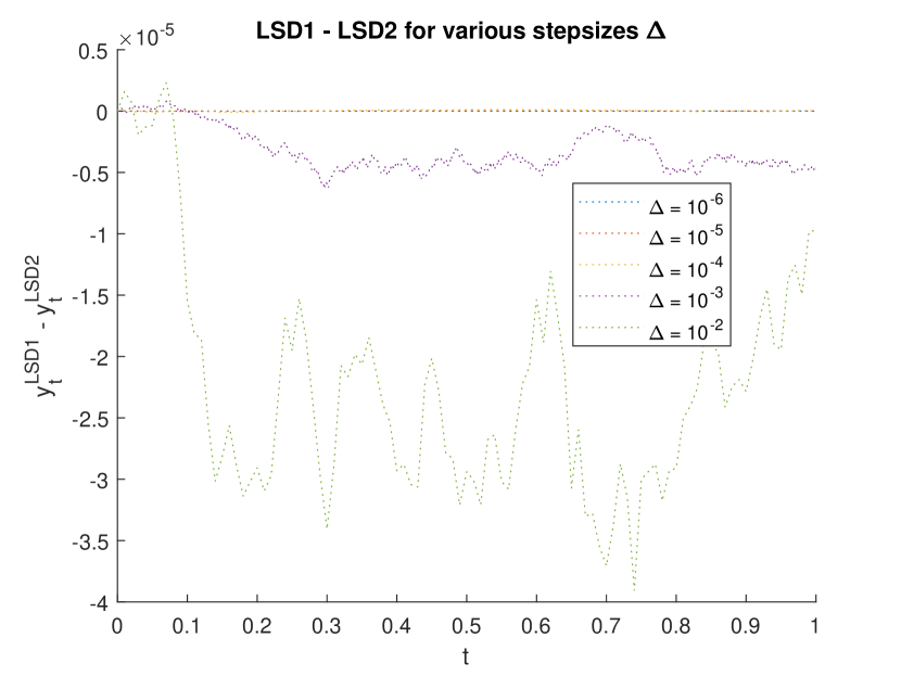
(c) LSD1 - LSD2

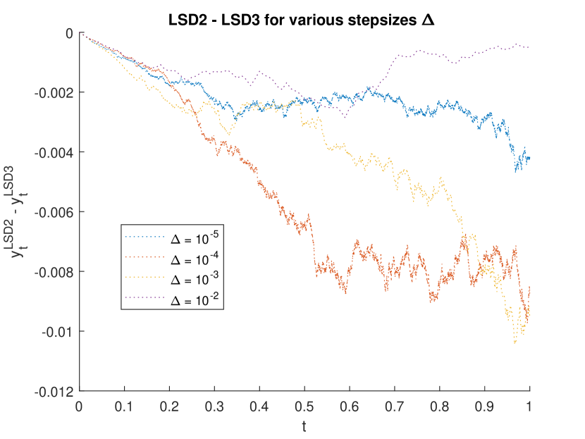
(d) LSD2 - LSD3

Figure 10. Trajectories of the differences of the numerical methods for the approximation of (25) with various step-sizes.

We also examine numerically the order of strong convergence of the LSD methods. The numerical results suggest that the LSD schemes converge in the mean-square sense with order close to $1,$ see Figure 11.

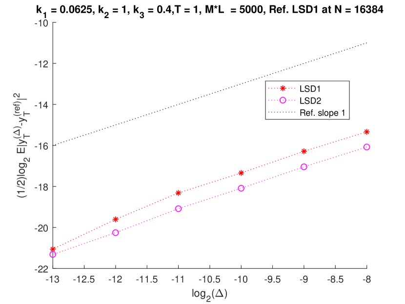
(a) LSD1 as reference solution

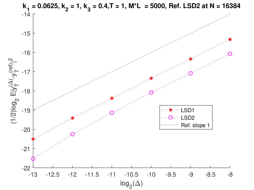
(b) LSD2 as reference solution

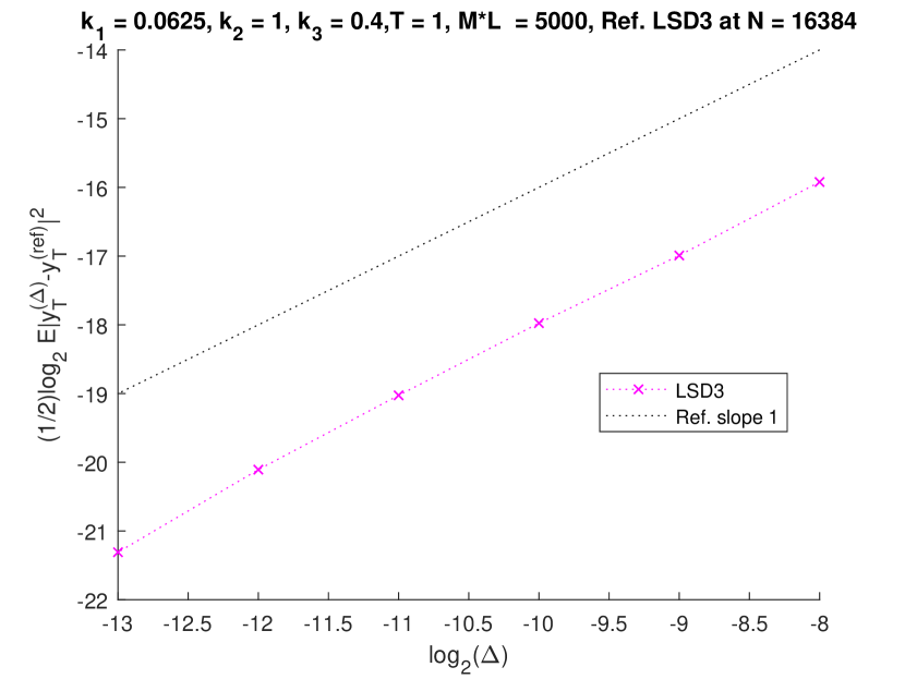
(c) LSD3 as reference solution

Figure 11. Convergence of (2.1), (2.2) and (2.2) for the approximation of (25) with different reference solutions.

3. Wright - Fisher model

Let

(42) $$x_{t}=x_{0}+\int_{0}^{t}(k_{1}-k_{2}x_{s})ds+k_{3}\int_{0}^{t}\sqrt{x_{s}(1-x_{s})}dW_{s},$$

where $k_{i}>0,i=1,2,3.$ If $x_{0}\in(0,1)$ and $2k_{1}\geq(k_{3})^{2},2(k_{2}-k_{1})\geq(k_{3})^{2},$ then $0<x_{t}<1$ a.s., see [9]. SDE (42) appears in population dynamics to describe fluctuations in gene frequency of reproducing individuals among finite populations [10] and ion channel dynamics within cardiac and neuronal cells, (c.f. [11], [12], [13] and references therein).

The transformed process $(z_{t})$ of (42) with $z=2\arcsin(\sqrt{x})$ has dynamics,

(43) $$z_{t} = z_{0}+\int_{0}^{t}\left(\left(k_{1}-\frac{(k_{3})^{2}}{4}\right)\cot(\frac{z_{s}}{2})-\left(k_{2}-k_{1}-\frac{(k_{3})^{2}}{4}\right)\tan(\frac{z_{s}}{2})\right)ds$$

$$+k_{3}\int_{0}^{t}dW_{s}.$$

Set $a:=k_{1}-\frac{(k_{3})^{2}}{4}$ and $b:=k_{2}-k_{1}-\frac{(k_{3})^{2}}{4}.$ The conditions on the parameters imply $a>0$ and $b>0.$ We consider three versions of the semi-discrete method for approximating (26). In the first version $(y_{t}),$ see Section 3.1, we use the standard semi-discrete method and in the other two versions $(\hat{y}_{t})$ and $(\widetilde{y}_{t})$ we study the new versions see Section 3.2, where in each subinterval $(t_{n},t_{n+1}]$ we solve an algebraic equation.

3.1. Lamperti Semi-Discrete method $\widetilde{z}^{1}_{n}$ for Wright-Fisher

Rewrite (43) as

(44) $$z_{t}=z_{0}+\int_{0}^{t}\left(a\cot(\frac{z_{s}}{2})-b\tan(\frac{z_{s}}{2})\right)ds+k_{3}\int_{0}^{t}dW_{s}.$$

For $t\in(t_{n},t_{n+1}]$ consider the process $(y_{t})$ where

(45) $$y_{t} = k_{3}\Delta W_{n}+y_{t_{n}}-b\tan(\frac{y_{t_{n}}}{2})\frac{y_{t}}{y_{t_{n}}}\Delta+\int_{t_{n}}^{t}a\cot(\frac{y_{s}}{2})ds$$

$$= \phi_{\Delta}(y_{t_{n}},\Delta W_{n})+\int_{t_{n}}^{t}\frac{a}{1+\frac{b}{y_{t_{n}}}\tan(\frac{y_{t_{n}}}{2})\Delta}\cot(\frac{y_{s}}{2})ds,$$

with $\hat{y}_{0}=z_{0}$ and $\phi_{\Delta}(x,y):=\frac{k_{3}y+x}{1+\frac{b}{x}\tan(x/2)\Delta}.$ Equation (45) has solution with the property, see Appendix C,

(46) $$|\cos(\frac{y_{t}}{2})|=|\cos(\frac{\phi_{\Delta}(y_{t_{n}},\Delta W_{n})}{2})|\exp\left\{-\frac{a/2}{1+\frac{b}{y_{t_{n}}}\tan(\frac{y_{t_{n}}}{2})\Delta}(t-t_{n})\right\}.$$

Note that $0<z_{t}<\pi$ a.s therefore since $(y_{t})$ converges to $(z_{t})$ the process $(y_{t})/2$ and belong to $(0,\pi/2).$ The proposed semi-discrete method $(y_{t})$ for the approximation of (43) satisfies

(47) $$\cos(\frac{y_{t_{n+1}}}{2})=|\cos(\frac{\phi_{\Delta}(y_{t_{n}},\Delta W_{n})}{2})|\exp\left\{-\frac{a\Delta/2}{1+\frac{b}{y_{t_{n}}}\tan(\frac{y_{t_{n}}}{2})\Delta}\right\},$$

which suggests the Lamperti semi-discrete method $(\widetilde{z}^{1}_{n})_{n\in{\mathbb{N}}}$ for the approximation of (42)

(48) $$\widetilde{z}^{1}_{t_{n+1}}=1-\cos^{2}(\frac{\phi_{\Delta}(y_{t_{n}},\Delta W_{n})}{2})\exp\left\{-\frac{a\Delta}{1+\frac{b}{y_{t_{n}}}\tan(\frac{y_{t_{n}}}{2})\Delta}\right\}.$$

Note that $(\widetilde{z}^{1}_{t_{n}})_{n\in{\mathbb{N}}}\in(0,1)$ when $x_{0}\in(0,1).$

3.2. Lamperti Semi-Discrete methods $\widetilde{z}^{2}_{n},\widetilde{z}^{3}_{n}$ and $\widetilde{z}^{4}_{n}$ for Wright-Fisher

For $t\in(t_{n},t_{n+1}]$ consider the processes $(\hat{y}_{t}),(\widetilde{y}_{t})$ and $(\bar{y}_{t})$ where

(49) $$\hat{y}_{t} = k_{3}(W_{t}-W_{t_{n}})+\hat{y}_{t_{n}}+\hat{y}_{t}\left(\frac{a}{\hat{y}_{t_{n}}}\cot(\frac{\hat{y}_{t_{n}}}{2})-\frac{b}{\hat{y}_{t_{n}}}\tan(\frac{\hat{y}_{t_{n}}}{2})\right)\Delta$$

$$= \frac{k_{3}(W_{t}-W_{t_{n}})+\hat{y}_{t_{n}}}{1-\frac{a}{\hat{y}_{t_{n}}}\cot(\frac{\hat{y}_{t_{n}}}{2})\Delta+\frac{b}{\hat{y}_{t_{n}}}\tan(\frac{\hat{y}_{t_{n}}}{2})\Delta},$$

with $\hat{y}_{0}=z_{0},$

(50) $$\widetilde{y}_{t} = k_{3}(W_{t}-W_{t_{n}})+\widetilde{y}_{t_{n}}+a\cot(\frac{\widetilde{y}_{t_{n}}}{2})\Delta-\frac{b}{\widetilde{y}_{t_{n}}}\tan(\frac{\widetilde{y}_{t_{n}}}{2})\Delta\widetilde{y}_{t}$$

$$= \frac{k_{3}(W_{t}-W_{t_{n}})+\widetilde{y}_{t_{n}}+a\cot(\frac{\widetilde{y}_{t_{n}}}{2})\Delta}{1+\frac{b}{\widetilde{y}_{t_{n}}}\tan(\frac{\widetilde{y}_{t_{n}}}{2})\Delta},$$

with $\widetilde{y}_{0}=z_{0}$ and

$$\bar{y}_{t}=k_{3}(W_{t}-W_{t_{n}})+\bar{y}_{t_{n}}+\left(a\cot(\frac{\bar{y}_{t_{n}}}{2})-b\tan(\frac{\bar{y}_{t_{n}}}{2})-\frac{1}{\bar{y}_{t_{n}}}\right)\Delta+\frac{\Delta}{\bar{y}_{t}}\\$$

with $\bar{y}_{0}=z_{0}.$ The solution of $(\bar{y}_{t})$ of the above equation satisfies

(51) $$(\bar{y}_{t})^{2}-\left(k_{3}(W_{t}-W_{t_{n}})+\bar{y}_{t_{n}}-\frac{\Delta}{\bar{y}_{t_{n}}}+\left(a\cot(\frac{\bar{y}_{t_{n}}}{2})-b\tan(\frac{\bar{y}_{t_{n}}}{2})\right)\Delta\right)(\bar{y}_{t})-\Delta=0.$$

The proposed semi-discrete methods $(\hat{y}_{t})$ and $(\widetilde{y}_{t})$ for the approximation of (43) read

(52) $$\hat{y}_{t_{n+1}}=\frac{k_{3}\Delta W_{n}+\hat{y}_{t_{n}}}{1-\frac{a}{\hat{y}_{t_{n}}}\cot(\frac{\hat{y}_{t_{n}}}{2})\Delta+\frac{b}{\hat{y}_{t_{n}}}\tan(\frac{\hat{y}_{t_{n}}}{2})\Delta}$$

and

(53) $$\widetilde{y}_{t_{n+1}}=\frac{k_{3}\Delta W_{n}+\widetilde{y}_{t_{n}}+a\cot(\frac{\widetilde{y}_{t_{n}}}{2})\Delta}{1+\frac{b}{\widetilde{y}_{t_{n}}}\tan(\frac{\widetilde{y}_{t_{n}}}{2})\Delta},$$

respectively, while for $(\bar{y}_{t})$ we have that

(54) $$\bar{y}_{t_{n+1}}=\frac{\bar{\phi}_{\Delta}(\bar{y}_{t_{n}},\Delta W_{n})+\sqrt{\bar{\phi}^{2}_{\Delta}(\bar{y}_{t_{n}},\Delta W_{n})+4\Delta}}{2},$$

with $\bar{\phi}_{\Delta}(x,y)=(k_{3}y+x-\Delta x^{-1}+a\left(\cot(x/2)-b\tan(x/2)\right)\Delta.$ Therefore, the versions of the Lamperti semi-discrete method $(\widetilde{z}^{2}_{n})_{n\in{\mathbb{N}}},(\widetilde{z}^{3}_{n})_{n\in{\mathbb{N}}}$ and $(\widetilde{z}^{4}_{n})_{n\in{\mathbb{N}}}$ for the approximation of (42) are

(55) $$\widetilde{z}^{2}_{t_{n+1}}=\sin^{2}\left(\frac{k_{3}\Delta W_{n}+\hat{y}_{t_{n}}}{2-\frac{2a}{\hat{y}_{t_{n}}}\cot(\frac{\hat{y}_{t_{n}}}{2})\Delta+\frac{2b}{\hat{y}_{t_{n}}}\tan(\frac{\hat{y}_{t_{n}}}{2})\Delta}\right),$$

(56) $$\widetilde{z}^{3}_{t_{n+1}}=\sin^{2}\left(\frac{k_{3}\Delta W_{n}+\widetilde{y}_{t_{n}}+a\cot(\frac{\widetilde{y}_{t_{n}}}{2})\Delta}{2+\frac{2b}{\widetilde{y}_{t_{n}}}\tan(\frac{\widetilde{y}_{t_{n}}}{2})\Delta}\right)$$

and

(57) $$\widetilde{z}^{4}_{t_{n+1}}=\sin^{2}\left(\frac{\bar{\phi}_{\Delta}(\bar{y}_{t_{n}},\Delta W_{n})+\sqrt{\bar{\phi}^{2}_{\Delta}(\bar{y}_{t_{n}},\Delta W_{n})+4\Delta}}{4}\right),$$

respectively. Note that $(\widetilde{z}^{j}_{t_{n}})_{n\in{\mathbb{N}}}\in(0,1),j=2,3,4$ when $x_{0}\in(0,1).$

3.3. Numerical experiment for Wright-Fisher

The semi-discrete method we proposed in [14] reads

(58) $$y_{t_{n+1}}=\sin^{2}\left(\frac{k_{3}}{2}\Delta W_{n}+\arcsin(\sqrt{\underbrace{y_{t_{n}}+\left(k_{1}-\frac{(k_{3})^{2}}{4}+y_{t_{n}}\left(\frac{(k_{3})^{2}}{2}-k_{2}\right)\right)\cdot\Delta}_{y_{n}}})\right),$$

which also possesses the qualitative property of domain preservation. Method (58) is well defined for all sufficiently small $\Delta$ such that $0<y_{n}<1.$ Let $\beta:=\frac{(k_{3})^{2}}{2}-k_{2}$ with $\beta<0.$ We require $\Delta$ small enough so that $0<y_{t_{n}}(1+\beta\Delta)+a\Delta.$ To simplify the conditions on $a,\beta,\Delta$, when necessary, we may adopt the strategy presented in [14] and consider the SD method

(59) $$\bar{y}_{t_{n+1}}=\sin^{2}\left(\frac{k_{3}}{2}\Delta W_{n}+\arcsin(\sqrt{\bar{y}_{n}})\right),$$

with

$$\bar{y}_{n}:=\frac{\bar{y}_{t_{n}}(1+\beta\Delta)+a\Delta}{1+(a+\beta)\Delta}.$$

The numerical scheme (59) is mean square convergent when $(k_{3})^{2}<2k_{2}$ for $\Delta<-1/\beta,$ see [14, Prop. 2.5] where the order of strong convergence was not theoretically proved.

The Balance Implicit Split Step (BISS) method suggested in [11, (4.8)] reads

(60) $$y_{n+1}^{BISS}=y_{n}+(k_{1}-k_{2}y_{n})\Delta+\frac{C\sqrt{y_{n}(1-y_{n})}\Delta W_{n}}{1+d^{1}(y_{n})|\Delta W_{n}|}(1-k_{2}\Delta),$$

where $\Delta$ is the step-size of the equidistant discretization of the interval $[0,1]$, the control function $d^{1}$ is given by

$$d^{1}(y)=\begin{cases}k_{3}\sqrt{(1-\varepsilon)/\varepsilon}\quad\,\text{if}\,\,y<\varepsilon,\\ k_{3}\sqrt{(1-y)/y}\quad\text{if}\,\,\varepsilon\leq y<1/2,\\ k_{3}\sqrt{y/(1-y)}\quad\text{if}\,\,1/2\leq y\leq 1-\varepsilon,\\ k_{3}\sqrt{(1-\varepsilon)/\varepsilon}\quad\,\text{if}\,\,y>1-\varepsilon,\end{cases}$$

and

$$\varepsilon=\min\{k_{1}\Delta,(k_{2}-k_{1})\Delta,1-k_{1}\Delta,1-(k_{2}-k_{1})\Delta\}.$$

The hybrid (HYB) scheme as proposed in [15, (11)] is the result of a splitting method and reads

(61) $$y_{n+1}^{HYB}=\frac{a}{\beta}(e^{\beta\Delta}-1)+e^{\beta\Delta}\sin^{2}\left(\frac{k_{3}}{2}\Delta W_{n}+\arcsin(\sqrt{y_{n}})\right).$$

with the restriction that

$$\frac{k_{1}}{k_{2}}\in\left(\frac{(k_{3})^{2}}{4k_{2}},1-\frac{(k_{3})^{2}}{4k_{2}}\right).$$

Moreover, we compare with the implicit method, see [6]. Set

$$G(x)=x-a\cot(x/2)\Delta-b(\tan(x/2))\Delta$$

and compute

$$y_{n+1}=G^{-1}(y_{n}+k_{3}\Delta W_{n})$$

and then transform back to get the following scheme

(62) $$y_{n+1}^{Impl}=\sin^{2}(y_{n+1}/2),$$

We use the set of parameters from [14, Sec.4] where all the methods work well, i.e. we take $(k_{1},k_{2},k_{3})=(1,2,0.20101),$ with $T=1$ and various step-sizes and compare the proposed versions of LSD schemes (48), (55), (56) and (57) with the BISS, the HYB, the SD method (58) and the implicit method (62). The initial condition is chosen to be the steady state of the deterministic part, i.e. $x_{0}=k_{1}/k_{2}.$

Figure 12 shows paths for the proposed LSD and existing numerical methods for the Wright -Fisher model and Figure 13 shows a graphical estimation of the difference of the methods.

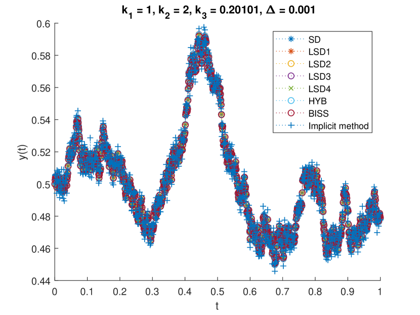
(a) With $\Delta=10^{-3}$.

(b) Zoom of Figure 12(A).

Figure 12. Trajectories of (48), (55), (56), (57), (58), (60), (61) and (62) for the approximation of (42).

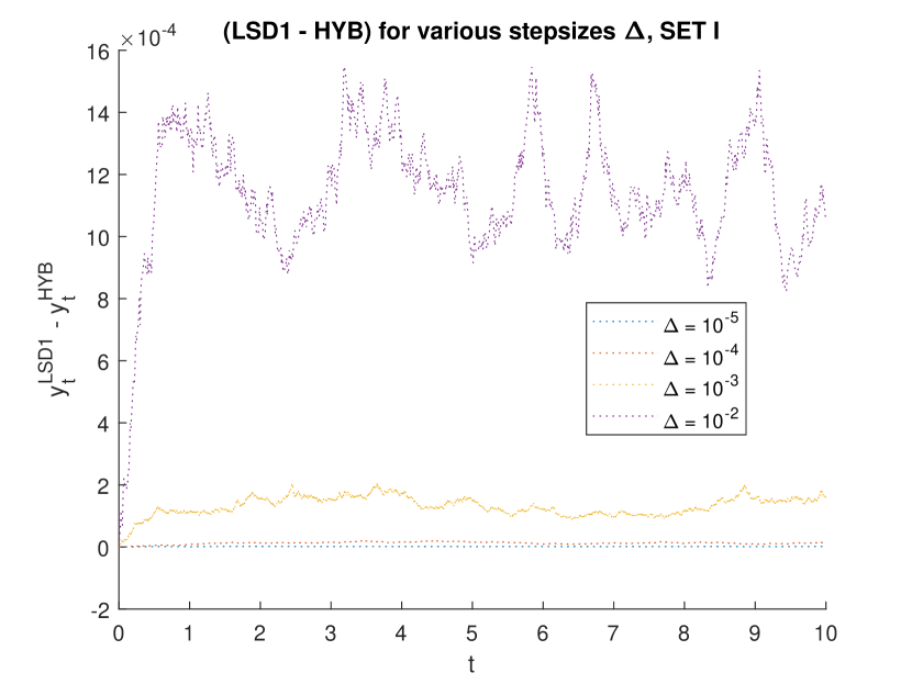
(a) LSD1 - HYB

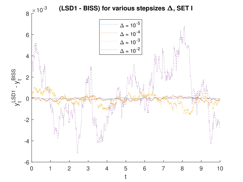
(b) LSD1 - BISS

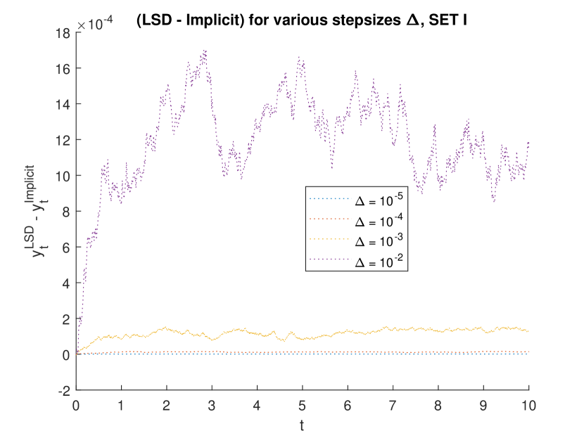
(c) LSD1 - Implicit

(d) LSD1 - SD

(e) LSD1 - LSD2

(f) LSD2 - LSD3

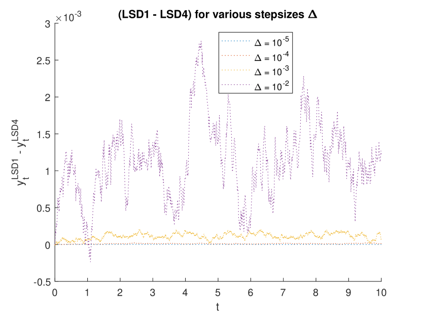
(g) LSD1 - LSD4

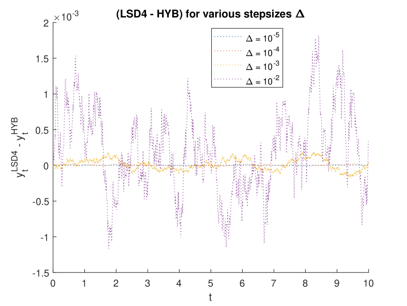
(h) LSD4 - HYB

Figure 13. Trajectories of the difference of numerical methods for the approximation of (42) with various $\Delta.$

We also examine numerically the order of strong convergence of the LSD method. The numerical results suggest that the LSD is mean-square convergent with order close to $1,$ see Figure 14.

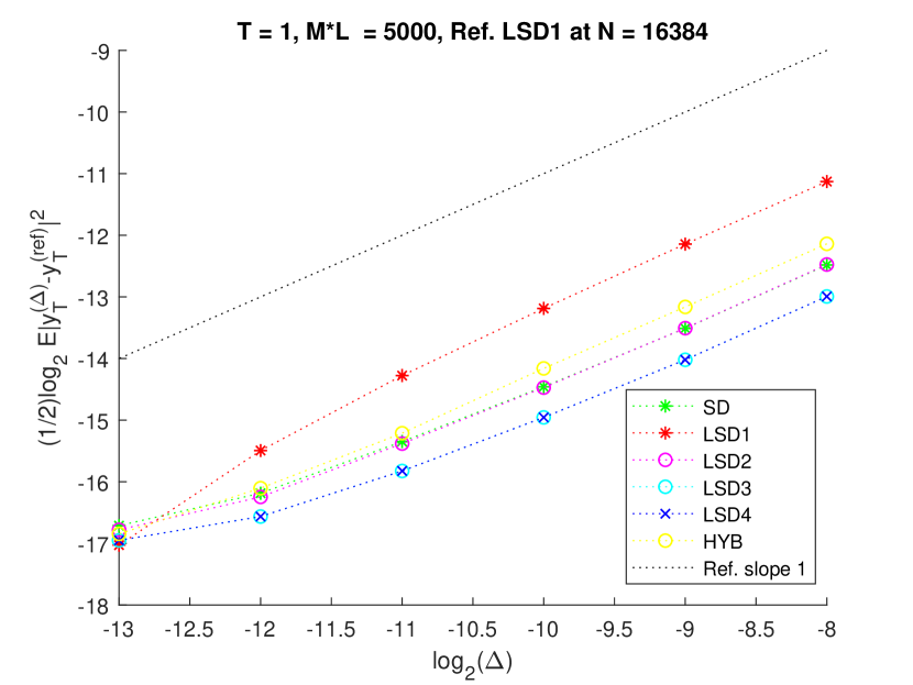
(a) LSD1 reference solution.

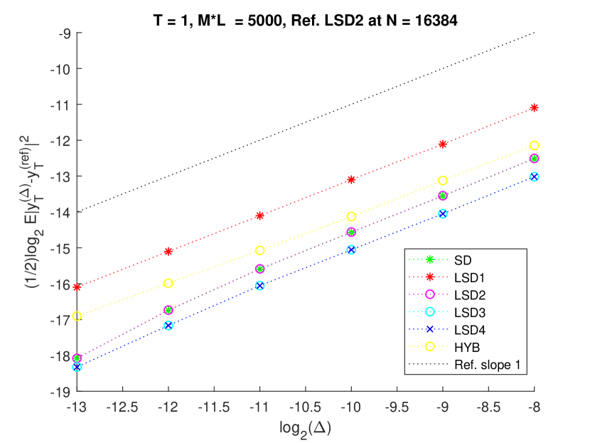
(b) LSD2 reference solution.

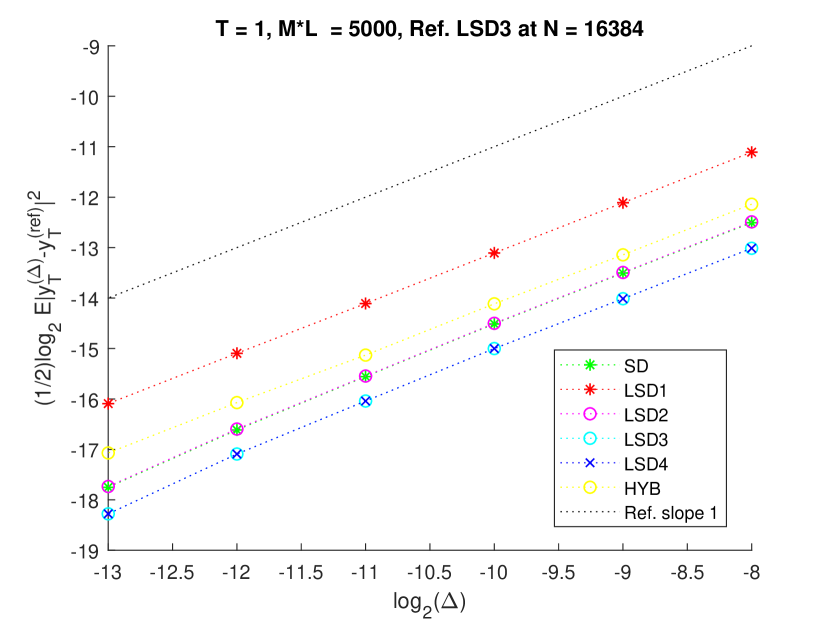
(c) LSD3 reference solution.

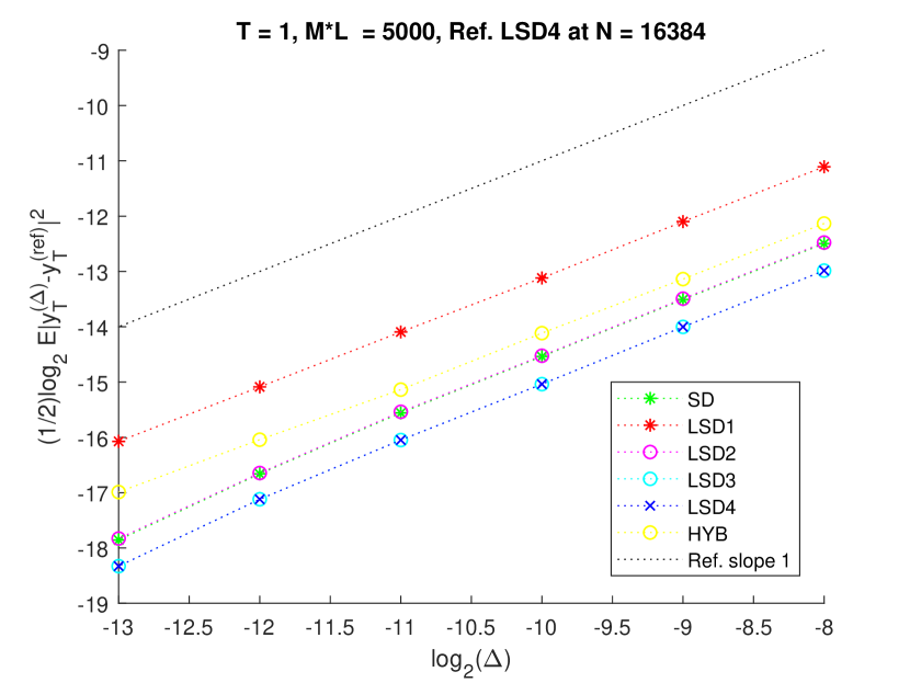
(d) LSD4 reference solution.

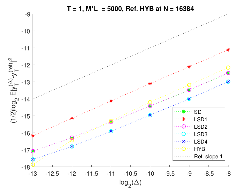
(e) HYB reference solution.

Figure 14. Convergence of LSD methods (48), (55), (56) and (57) for the approximation of (42) with different reference solutions.

4. Heston $3/2$-model

Let

(63) $$x_{t}=x_{0}+\int_{0}^{t}(k_{1}x_{s}-k_{2}(x_{s})^{2})ds+\int_{0}^{t}k_{3}(x_{s})^{3/2}dW_{s},\quad t\geq 0,$$

where the coefficients $k_{i},i=1,2,3$ are positive and $x_{0}>0.$ SDE (63) is known as the Heston $3/2$-model appearing in financial mathematics as a stochastic volatility process, see [16], and satisfies $x_{t}>0$ a.s. The Lamperti transformation of (63) is $z=\frac{2}{k_{3}}x^{-1/2}$ implying that, see Appendix A,

(64) $$z_{t}=z_{0}+\int_{0}^{t}\left((\frac{2k_{2}}{(k_{3})^{2}}+3)(z_{s})^{-1}-\frac{k_{1}}{2}z_{s}\right)ds+\int_{0}^{t}dW_{s},\,\,t\geq 0.$$

4.1. Lamperti Semi-Discrete method $\widetilde{z}^{1}_{n}$ and $\widetilde{z}^{2}_{n}$ for Heston $3/2$-model

As in Section 1.1 we consider the following two versions of the semi-discrete method for approximating (64),

(65) $$y_{t}=\Delta W_{n}+y_{t_{n}}-\frac{k_{1}}{2}y_{t_{n}}\Delta+\int_{t_{n}}^{t}(\frac{2k_{2}}{(k_{3})^{2}}+3)(y_{s})^{-1}ds,\,\,t\in(t_{n},t_{n+1}],$$

with $y_{0}=z_{0}$ and

(66) $$\hat{y}_{t}=\Delta W_{n}+\hat{y}_{t_{n}}+\int_{t_{n}}^{t}\left((\frac{2k_{2}}{(k_{3})^{2}}+3)(\hat{y}_{s})^{-1}-\frac{k_{1}}{2}\hat{y}_{s}\right)ds,\,\,t\in(t_{n},t_{n+1}],$$

with $\hat{y}_{0}=z_{0}.$ (65) and (66) are Bernoulli type equations with solutions satisfying, see Appendix B,

(67) $$(y_{t})^{2}=\left(\Delta W_{n}+\left(1-\frac{k_{1}\Delta}{2}\right)y_{t_{n}}\right)^{2}+(\frac{4k_{2}}{(k_{3})^{2}}+6)(t-t_{n})$$

and

(68) $$(\hat{y}_{t})^{2}=(\Delta W_{n}+\hat{y}_{t_{n}})^{2}e^{-k_{1}(t-t_{n})}+(\frac{4k_{2}}{(k_{3})^{2}}+6)\frac{1-e^{-k_{1}(t-t_{n})}}{k_{1}},$$

respectively. We propose the following versions of the semi-discrete method for the approximation of (2),

(69) $$y_{t_{n+1}}=\sqrt{\left(\Delta W_{n}+\left(1-\frac{k_{1}\Delta}{2}\right)y_{t_{n}}\right)^{2}+(\frac{4k_{2}}{(k_{3})^{2}}+6)\Delta}$$

and

(70) $$\hat{y}_{t_{n+1}}=\sqrt{(\Delta W_{n}+\hat{y}_{t_{n}})^{2}e^{-k_{1}\Delta}+(\frac{4k_{2}}{(k_{3})^{2}}+6)\frac{1-e^{-k_{1}\Delta}}{k_{1}}},$$

which suggests the versions of the Lamperti semi-discrete method $(\widetilde{z}_{n})_{n\in{\mathbb{N}}}$ for the approximation of (1)

(71) $$\widetilde{z}^{1}_{t_{n+1}}=\frac{4}{(k_{3})^{2}}\left(\left(\Delta W_{n}+\left(1-\frac{k_{1}\Delta}{2}\right)y_{t_{n}}\right)^{2}+(\frac{4k_{2}}{(k_{3})^{2}}+6)\Delta\right)^{-1}$$

(72) $$\widetilde{z}^{2}_{t_{n+1}}=\frac{4}{(k_{3})^{2}}\left((\Delta W_{n}+\hat{y}_{t_{n}})^{2}e^{-k_{1}\Delta}+(\frac{4k_{2}}{(k_{3})^{2}}+6)\frac{1-e^{-k_{1}\Delta}}{k_{1}}\right)^{-1}$$

4.2. Numerical experiment for Heston $3/2$-model

For a minimal numerical experiment we present simulation paths for the numerical approximation of (63) with $x_{0}=1$ and compare with the SD method proposed in [17, Sec. 5], which reads

(73) $$\widetilde{y}_{t_{n+1}}=\widetilde{y}_{t_{n}}\exp\left\{\left(k_{1}-k_{2}\widetilde{y}_{t_{n}}-\frac{(k_{3})^{2}}{2}\widetilde{y}_{t_{n}}\right)\Delta+k_{3}\sqrt{\widetilde{y}_{t_{n}}}\Delta W_{n}\right\}.$$

The semi-discrete method (73) is strongly converging and positivity preserving, see [17, Sec. 5].

Moreover, we compare with the implicit method proposed in [6]. Set

$$G(x)=\left(1+\frac{k_{1}}{2}\Delta\right)x-\left(\frac{k_{2}}{2}+\frac{3(k_{3})^{2}}{8}\right)\Delta x^{-1}$$

and compute

$$y_{n+1}=G^{-1}\left(y_{n}-\frac{k_{3}}{2}\Delta W_{n}\right)$$

and then transform back to get the following scheme

(74) $$y_{n+1}^{Impl}=(y_{n+1})^{-2}.$$

We use the set of parameters from [17, Sec.5]; we take $k_{1}=0.1,k_{2}=70,k_{3}=\sqrt{0.2},T=1$ with various step-sizes. We compare the proposed two versions of LSD scheme (71) and (72) with the SD scheme (73) and the implicit method (74). Figure 15 shows that the pair of LSD1 and LSD2 and the pair of SD with the implicit method are almost identical for a step-size $\Delta=10^{-4}.$ Moreover, the two pairs are getting very close. We give a presentation of the difference of the various approximations in Figure 16.

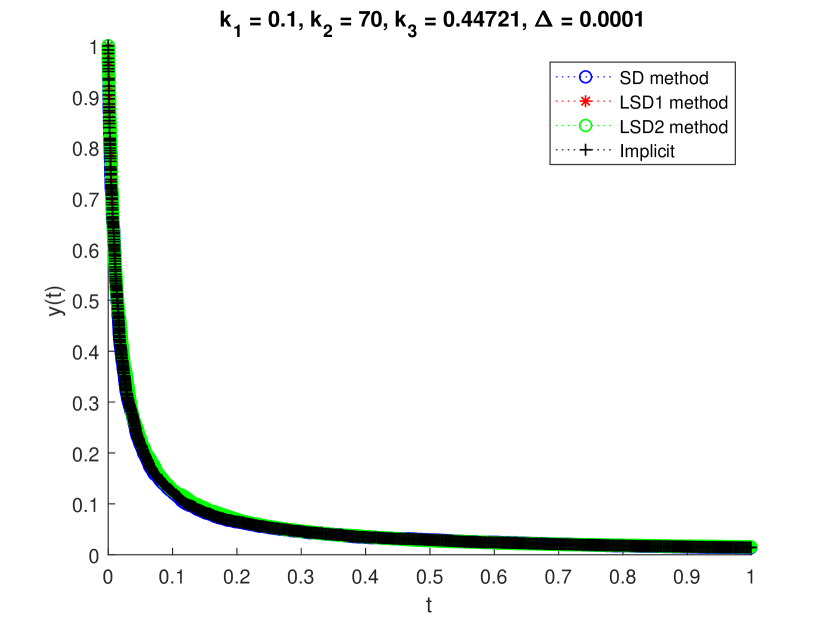
(a) Trajectories of (71)-(74).

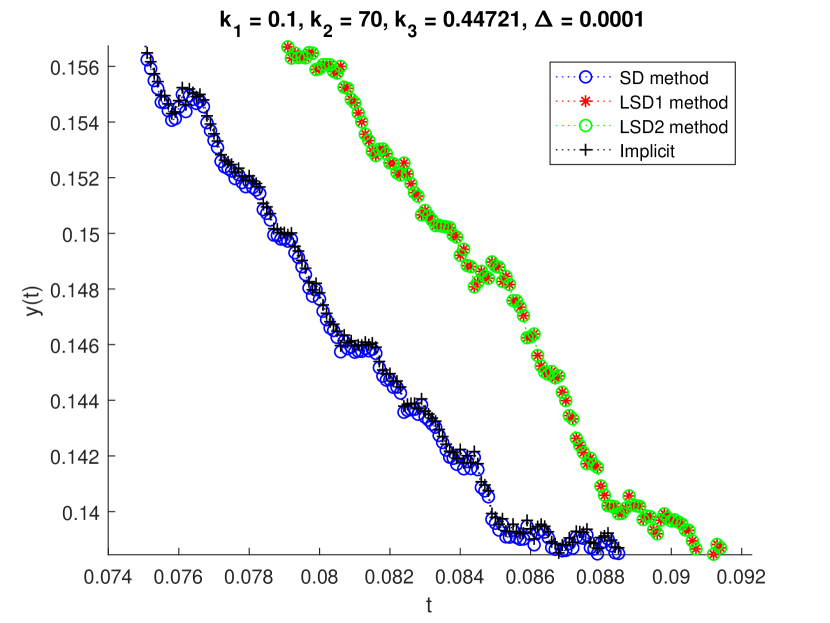
(b) Zoom of Figure 15(A).

Figure 15. Trajectories of (71), (72), (73) and (74) for the approximation of (63) with $\Delta=10^{-4}$.

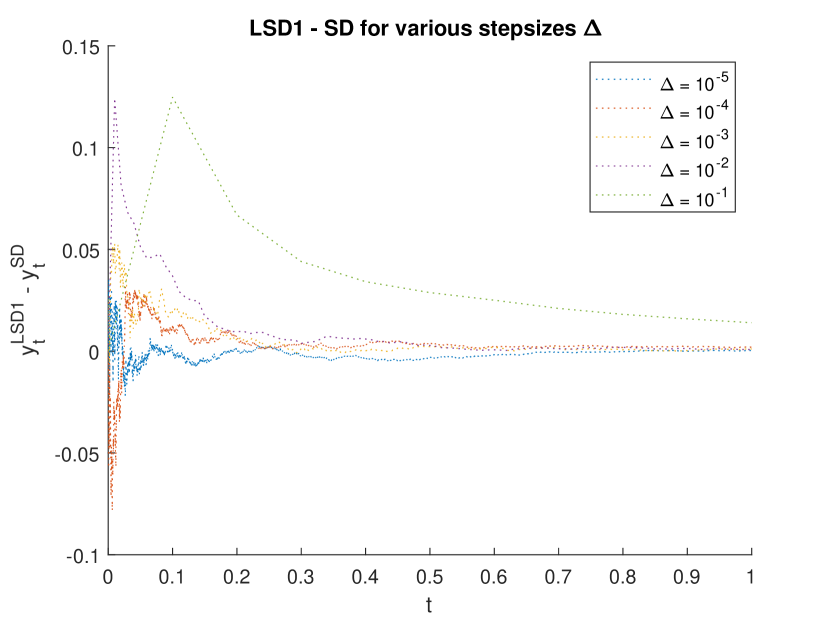
(a) Difference (71) - (73) for various step sizes.

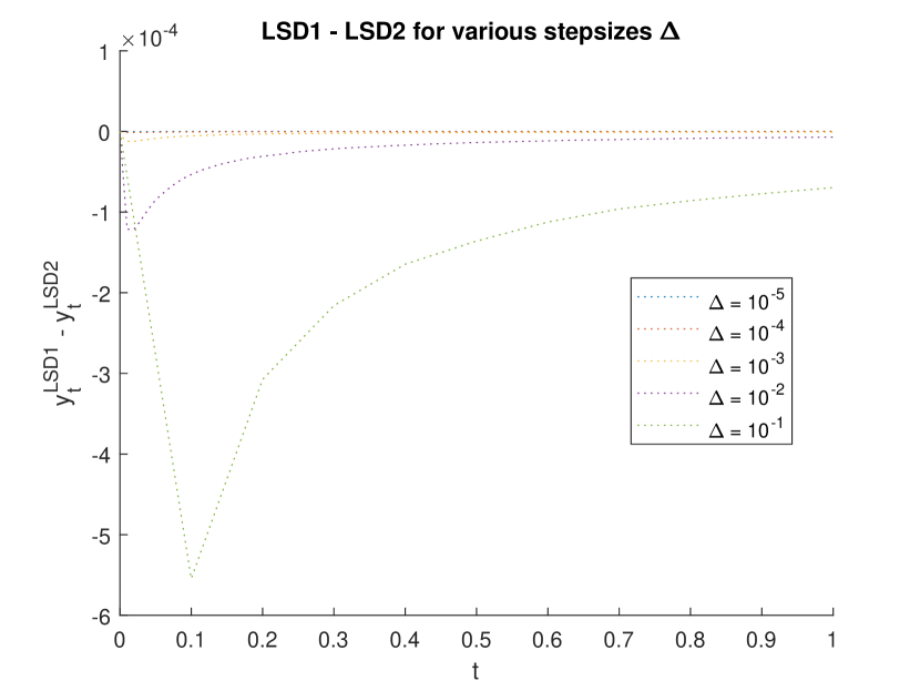
(b) Difference (71) - (72) for various step sizes.

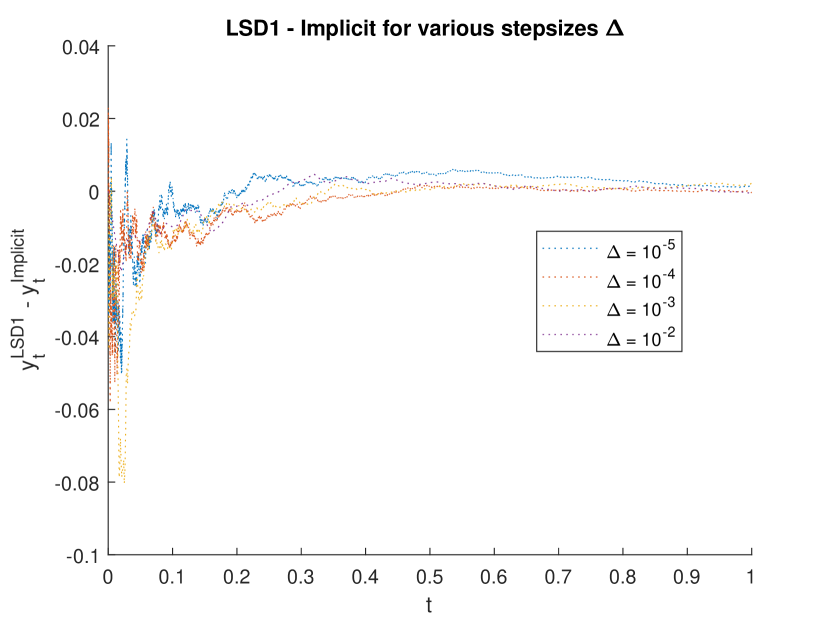
(c) Difference (71) - (74) for various step sizes.

Figure 16. Trajectories of the differences of the semi-discrete methods (71), (72), (73) and the implicit scheme (74) for the approximation of (63) with various step-sizes.

Finally, we examine numerically the order of strong convergence of the LSD method. The numerical results suggest that the LSD1 scheme as well as LSD2 converge in the mean-square sense with order close to $1,$ see Figure 17.

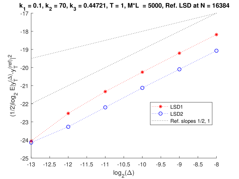
(a) LSD1 as reference solution.

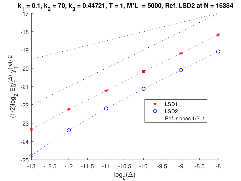
(b) LSD2 as reference solution.

Figure 17. Convergence of LSD1 and LSD2 method (71) and (71) for the approximation of (63) with different reference solution.

5. Aït-Sahalia model

Let

(75) $$x_{t}=x_{0}+\int_{0}^{t}(k_{-1}(x_{s})^{-1}-k_{0}+k_{1}x_{s}-k_{2}(x_{s})^{r})ds+\int_{0}^{t}k_{3}(x_{s})^{\rho}dW_{s},\quad t\geq 0.$$

where $k_{-1},k_{0},k_{1},k_{2}$ and $k_{3}$ are positive constants with $r>1$ and $\rho>1.$ SDE (5) is an Aït-Sahalia model with superlinear coefficients and the property $x_{t}>0$ a.s. The Lamperti transformation of (75) is $z=x^{1-\rho}$ with dynamics, see Appendix A,

(76) $$z_{t} = z_{0}+\int_{0}^{t}\Big{(}k_{-1}(1-\rho)(z_{s})^{\frac{\rho+1}{\rho-1}}-k_{0}(1-\rho)(z_{s})^{\frac{\rho}{\rho-1}}+k_{1}(1-\rho)z_{s}$$

$$-k_{2}(1-\rho)(z_{s})^{\frac{\rho-r}{\rho-1}}-\frac{\rho(1-\rho)(k_{3})^{2}}{2}(z_{s})^{-1}\Big{)}ds+\int_{0}^{t}k_{3}(1-\rho)dW_{s}.$$

Set $K_{i}=k_{i}(\rho-1),i=-1,\dots,3$ and $K_{4}=\frac{\rho(\rho-1)(k_{3})^{2}}{2}.$ We examine the new version $(y_{t}),$ of the semi-discrete method for approximating (76) see Section 5.1, where in each subinterval $(t_{n},t_{n+1}]$ we solve an algebraic equation, producing a positive numerical scheme.

5.1. Lamperti Semi-Discrete methods $\widetilde{z}^{1}_{n},\widetilde{z}^{2}_{n}$ for Aït-Sahalia

Rewrite (76) as

(77) $$z_{t} = z_{0}+\int_{0}^{t}\left(-K_{-1}(z_{s})^{\frac{\rho+1}{\rho-1}}+K_{0}(z_{s})^{\frac{\rho}{\rho-1}}-K_{1}z_{s}+K_{2}(z_{s})^{\frac{\rho-r}{\rho-1}}+K_{4}(z_{s})^{-1}\right)ds$$

$$\qquad\quad-\int_{0}^{t}K_{3}dW_{s}.$$

Let $t\in(t_{n},t_{n+1}]$ and

(78) $$y_{t} = -K_{3}(W_{t}-W_{t_{n}})+y_{t_{n}}-K_{-1}(y_{t_{n}})^{\frac{2}{\rho-1}}y_{t}\Delta+K_{0}(y_{t_{n}})^{\frac{\rho}{\rho-1}}\Delta-K_{1}y_{t}\Delta$$

$$+K_{2}(y_{t_{n}})^{\frac{2\rho-r-1}{\rho-1}}(y_{t})^{-1}\Delta+K_{4}(y_{t})^{-1}\Delta$$

with $y_{0}=z_{0}$ and

(79) $$\hat{y}_{t} = -K_{3}(W_{t}-W_{t_{n}})+\hat{y}_{t_{n}}-K_{-1}(\hat{y}_{t_{n}})^{\frac{\rho+1}{\rho-1}}\Delta+K_{0}(\hat{y}_{t_{n}})^{\frac{\rho}{\rho-1}}\Delta-K_{1}\hat{y}_{t}\Delta$$

$$+K_{2}(\hat{y}_{t_{n}})^{\frac{2\rho-r-1}{\rho-1}}(\hat{y}_{t})^{-1}\Delta+K_{4}(\hat{y}_{t})^{-1}\Delta$$

with $\hat{y}_{0}=z_{0}.$ The solutions of (78) and (79) are such that

$$(1+K_{-1}(y_{t_{n}})^{\frac{2}{\rho-1}}\Delta+K_{1}\Delta)(y_{t})^{2}-\left(-K_{3}(W_{t}-W_{t_{n}})+y_{t_{n}}+K_{0}(y_{t_{n}})^{\frac{\rho}{\rho-1}}\Delta\right)y_{t}$$

(80) $$\qquad\qquad\quad-\left(K_{2}(y_{t_{n}})^{\frac{2\rho-r-1}{\rho-1}}+K_{4}\right)\Delta=0$$

and

$$(1+K_{1}\Delta)(\hat{y}_{t})^{2}-\left(-K_{3}(W_{t}-W_{t_{n}})+\hat{y}_{t_{n}}+K_{0}(\hat{y}_{t_{n}})^{\frac{\rho}{\rho-1}}\Delta-K_{-1}(\hat{y}_{t_{n}})^{\frac{\rho+1}{\rho-1}}\Delta\right)\hat{y}_{t}$$

(81) $$\qquad\qquad\quad-\left(K_{2}(\hat{y}_{t_{n}})^{\frac{2\rho-r-1}{\rho-1}}+K_{4}\right)\Delta=0$$

respectively.

We propose the following versions of the semi-discrete method for the approximation of (77),

(82) $$y_{t_{n+1}}=\frac{\phi_{\Delta}(y_{t_{n}},\Delta W_{n})+\sqrt{\phi^{2}_{\Delta}(y_{t_{n}},\Delta W_{n})+4C_{1}(y_{t_{n}})C_{2}(y_{t_{n}})}}{2C_{1}(y_{t_{n}})},$$

with $\phi_{\Delta}(x,y)=-K_{3}y+x+K_{0}x^{\frac{\rho}{\rho-1}}\Delta,C_{1}(x)=(1+K_{-1}x^{\frac{2}{\rho-1}}\Delta+K_{1}\Delta)$ and $C_{2}(x)=\left(K_{2}x^{\frac{2\rho-r-1}{\rho-1}}+K_{4}\right)\Delta$ and

(83) $$\hat{y}_{t_{n+1}}=\frac{\hat{\phi}_{\Delta}(\hat{y}_{t_{n}},\Delta W_{n})+\sqrt{\hat{\phi}^{2}_{\Delta}(\hat{y}_{t_{n}},\Delta W_{n})+4(1+K_{1}\Delta)C_{2}(\hat{y}_{t_{n}})}}{2(1+K_{1}\Delta)},$$

with $\hat{\phi}_{\Delta}(x,y)=\phi_{\Delta}(x,y)-K_{-1}x^{\frac{\rho+1}{\rho-1}}\Delta,$ which suggests the versions of the Lamperti semi-discrete method $(\widetilde{z}^{1}_{n})_{n\in{\mathbb{N}}}$ and $(\widetilde{z}^{2}_{n})_{n\in{\mathbb{N}}}$ for the approximation of (75) with $\widetilde{z}^{1}_{n}=(y_{n})^{1/(1-\rho)},\widetilde{z}^{2}_{n}=(\hat{y}_{n})^{1/(1-\rho)}$ or

(84) $$\widetilde{z}^{1}_{t_{n+1}}=\left|\frac{\phi_{\Delta}(y_{t_{n}},\Delta W_{n})+\sqrt{\phi^{2}_{\Delta}(y_{t_{n}},\Delta W_{n})+4C_{1}(y_{t_{n}})C_{2}(y_{t_{n}})}}{2C_{1}(y_{t_{n}})}\right|^{\frac{1}{1-\rho}}.$$

(85) $$\widetilde{z}^{2}_{t_{n+1}}=\left|\frac{\hat{\phi}_{\Delta}(\hat{y}_{t_{n}},\Delta W_{n})+\sqrt{\hat{\phi}^{2}_{\Delta}(\hat{y}_{t_{n}},\Delta W_{n})+4(1+K_{1}\Delta)C_{2}(\hat{y}_{t_{n}})}}{2(1+K_{1}\Delta)}\right|^{\frac{1}{1-\rho}}.$$

5.2. Numerical experiment for Aït-Sahalia

For a minimal numerical experiment we present simulation paths for the numerical approximation of (75) with $x_{0}=4$ and compare with the implicit method proposed in [6]. Set

$$G(x)=x+\left(1+K_{-1}x^{\frac{\rho+1}{\rho-1}}-K_{0}x^{\frac{\rho}{\rho-1}}+K_{1}x-K_{2}x^{\frac{\rho-r}{\rho-1}}+K_{4}x^{-1}\right)\Delta$$

and compute

$$y_{n+1}=G^{-1}\left(y_{n}-K_{3}\Delta W_{n}\right)$$

and then transform back to get the following scheme

(86) $$y_{n+1}^{Impl}=(y_{n+1})^{1/(1-\rho)}.$$

We use a set of parameters so that (86) works; we take the coefficients $k_{-1}=2,k_{0}=3,k_{1}=4,k_{2}=6,k_{3}=1$ the exponents $r=2$ and $\rho=3/2$ and $T=1.$ We compare the proposed versions of LSD schemes (84) and (85) with the implicit method (86). Figure 18 shows that the LSD1 and LSD2 are very close to the implicit method. We give a presentation of the difference of the two methods in Figure 16.

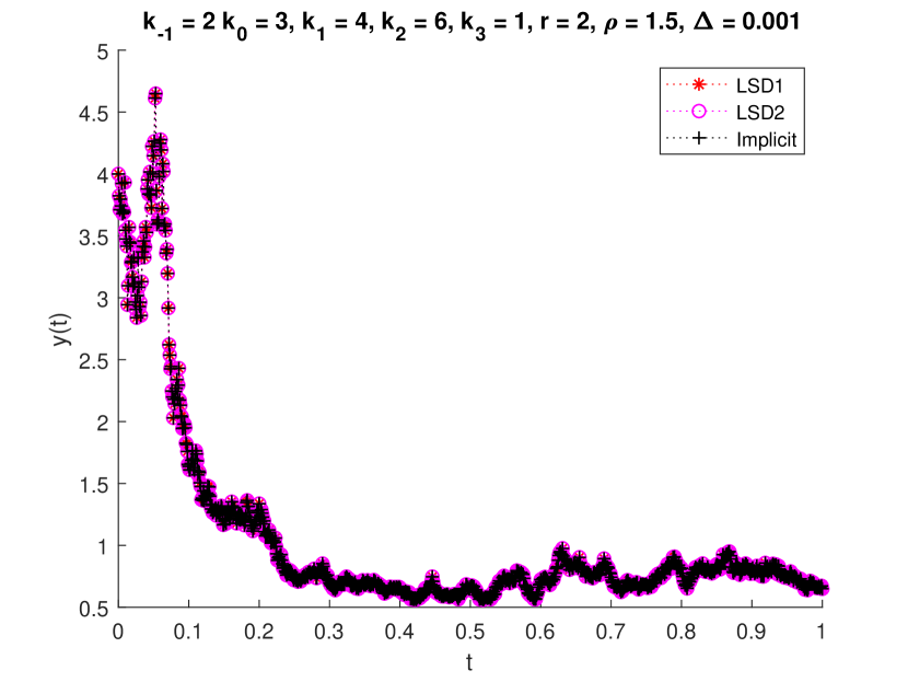
(a) A path with $\Delta=10^{-3}$.

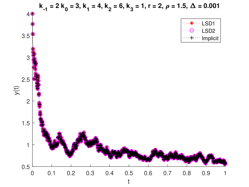
(b) A path with $\Delta=10^{-3}$.

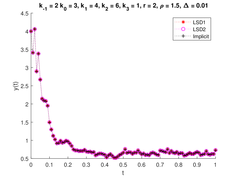
(c) A path with $\Delta=10^{-2}$.

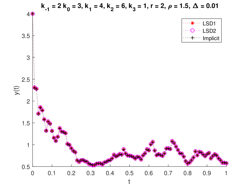
(d) A path with $\Delta=10^{-2}$.

Figure 18. Trajectories of (84), (85) and (86) for the approximation of (75) with various $\Delta$.

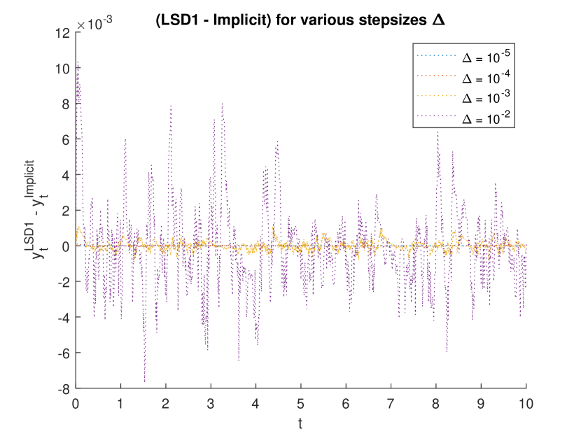
(a) (84) - (86)

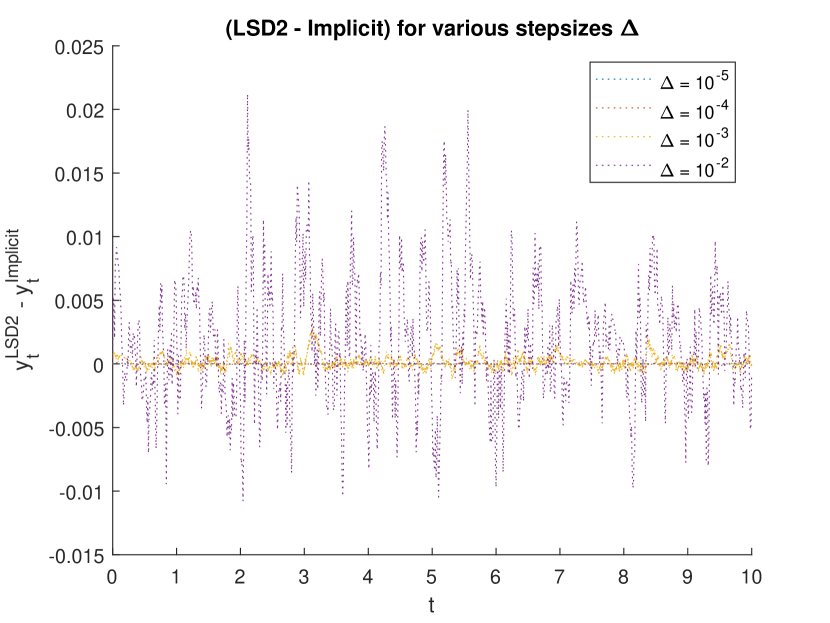
(b) (85) - (86)

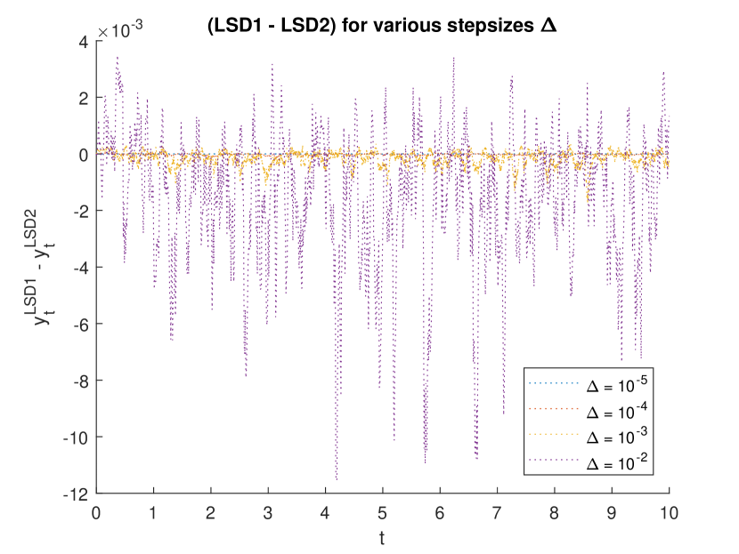
(c) (84) - (86)

Figure 19. Differences between (84), (85) and (86) for the approximation of (75) with various step-sizes.

Finally, we examine numerically the order of strong convergence of the LSD method. The numerical results suggest that the LSD1 and LSD2 schemes converge in the mean-square sense with order close to $1,$ see Figure 20.

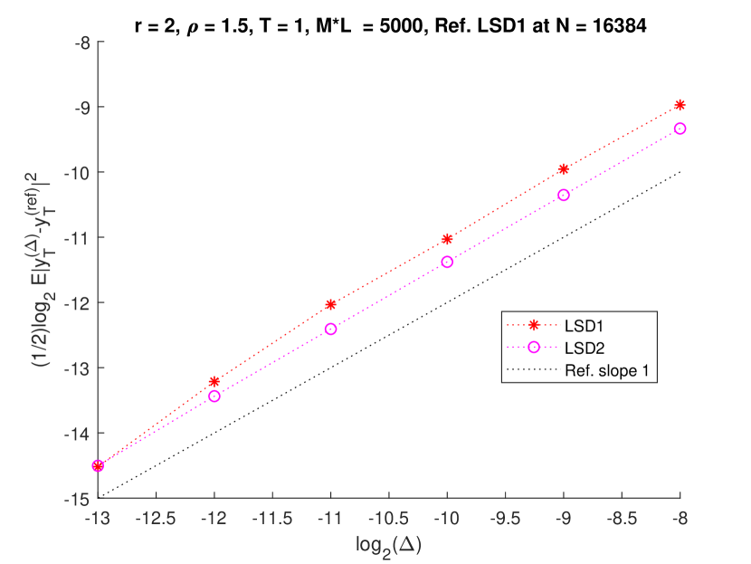
(a) LSD1 as reference solution

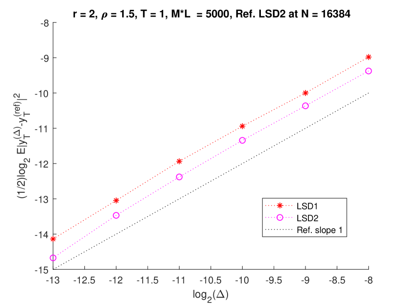
(b) LSD2 as reference solution

Figure 20. Convergence of LSD methods (84 and (85) for the approximation of (75) with different reference solutions.

Appendix A Lamperti Tranformation of (1), (63), (75)

Applying the Itô formula to the transformation $z(x)=\frac{2}{k_{3}}\sqrt{x}$ of (1) we obtain

$$dz_{t} = \left(\frac{1}{k_{3}}(x_{t})^{-1/2}(k_{1}-k_{2}x_{t})+\frac{1}{k_{3}}\frac{1}{2}(-\frac{1}{2})(x_{t})^{-3/2}(k_{3})^{2}(x_{t})\right)dt+\frac{1}{k_{3}}(x_{t})^{-1/2}k_{3}(x_{t})^{1/2}dW_{t}$$

$$= \left(\frac{k_{1}}{k_{3}}(x_{t})^{-1/2}-(\frac{k_{2}}{k_{3}}+\frac{1}{4}k_{3})\sqrt{x_{t}}\right)dt+dW_{t}$$

$$= \left(\frac{2k_{1}}{(k_{3})^{2}}(z_{t})^{-1}-(\frac{k_{2}}{2}+\frac{(k_{3})^{2}}{8})z_{t}\right)dt+dW_{t},$$

or for $t\geq t_{0}$

$$z_{t} = z_{t_{0}}+\int_{t_{0}}^{t}\left(\frac{2k_{1}}{(k_{3})^{2}}(z_{s})^{-1}-(\frac{k_{2}}{2}+\frac{(k_{3})^{2}}{8})z_{s}\right)ds+\int_{t_{0}}^{t}dW_{s}$$

$$= z_{t_{0}}+\int_{t_{0}}^{t}\left(\frac{2k_{1}}{(k_{3})^{2}}(z_{s})^{-1}-(\frac{k_{2}}{2}+\frac{(k_{3})^{2}}{8})z_{s}\right)ds+W_{t}-W_{t_{0}}.$$

Analogously, the transformation $z(x)=\frac{2}{k_{3}}(x)^{-1/2}$ of (63) has the following dynamics,

$$dz_{t} = \left(\frac{-1}{k_{3}}(x_{t})^{-3/2}(k_{1}x_{t}-k_{2}(x_{t})^{2})+\frac{3}{4k_{3}}(x_{t})^{-5/2}(k_{3})^{2}(x_{t})^{3}\right)dt+\frac{-1}{k_{3}}(x_{t})^{-3/2}k_{3}(x_{t})^{3/2}dW_{t}$$

$$= \left(-\frac{k_{1}}{k_{3}}(x_{t})^{-1/2}+(\frac{k_{2}}{k_{3}}+\frac{3}{2}k_{3})\sqrt{x_{t}}\right)dt+dW_{t}$$

$$= \left((\frac{2k_{2}}{(k_{3})^{2}}+3)(z_{t})^{-1}-\frac{k_{1}}{2}z_{t}\right)dt+dW_{t},$$

or for $t\geq t_{0},$

$$z_{t}=z_{t_{0}}+\int_{t_{0}}^{t}\left((\frac{2k_{2}}{(k_{3})^{2}}+3)(z_{s})^{-1}-\frac{k_{1}}{2}z_{s}\right)ds+W_{t}-W_{t_{0}}.$$

Finally, the transformation $z(x)=x^{1-\rho}$ of (75) is such that

$$dz_{t} = \left((1-\rho)(x_{t})^{-\rho}(k_{-1}(x_{t})^{-1}-k_{0}+k_{1}x_{t}-k_{2}(x_{t})^{r})-\frac{\rho(1-\rho)(k_{3})^{2}}{2}(x_{t})^{\rho+1}\right)dt$$

$$+k_{3}(1-\rho)(x_{t})^{-\rho}(x_{t})^{\rho}dW_{t}$$

$$= (1-\rho)\left(k_{-1}(x_{t})^{-\rho-1}-k_{0}(x_{t})^{-\rho}+k_{1}(x_{t})^{-\rho+1}-k_{2}(x_{t})^{-\rho+r}-\frac{\rho(1-\rho)(k_{3})^{2}}{2}(x_{t})^{\rho+1}\right)dt$$

$$+k_{3}(1-\rho)dW_{t}$$

$$= (1-\rho)\left(k_{-1}(z_{t})^{\frac{\rho+1}{\rho-1}}-k_{0}(z_{t})^{\frac{\rho}{\rho-1}}+k_{1}z_{t}-k_{2}(z_{t})^{-\frac{r-\rho}{\rho-1}}-\frac{\rho(1-\rho)(k_{3})^{2}}{2}(z_{t})^{-1}\right)dt$$

$$+k_{3}(1-\rho)dW_{t},$$

or for $t\geq t_{0},$

$$z_{t} = z_{t_{0}}+\int_{t_{0}}^{t}\Big{(}k_{-1}(1-\rho)(z_{s})^{\frac{\rho+1}{\rho-1}}-k_{0}(1-\rho)(z_{s})^{\frac{\rho}{\rho-1}}+k_{1}(1-\rho)z_{s}$$

$$-k_{2}(1-\rho)(z_{s})^{\frac{\rho-r}{\rho-1}}-\frac{\rho(1-\rho)(k_{3})^{2}}{2}(z_{s})^{-1}\Big{)}ds+k_{3}(1-\rho)(W_{t}-W_{t_{0}}).$$

Appendix B Solution of Bernoulli equations (4), (5), (28)

Consider the following differential equation

(87) $$y_{t}=A_{n}+\int_{t_{n}}^{t}\left(B_{n}(y_{s})^{-l}+C_{n}y_{s}\right)ds,$$

with $l>0.$ The dynamics for the transformation $r=y^{1+l}$ are

$$dr_{t}=\left((1+l)B_{n}+(1+l)C_{n}r_{t}\right)dt,$$

that is a linear equation with solution

$$r_{t} = \frac{\int_{t_{n}}^{t}e^{-(1+l)C_{n}(s-t_{n})}(1+l)B_{n}ds+(A_{n})^{1+l}}{e^{-(1+l)C_{n}(t-t_{n})}}$$

$$= (1+l)B_{n}e^{(1+l)C_{n}t}\int_{t_{n}}^{t}e^{-(1+l)C_{n}s}ds+(A_{n})^{1+l}e^{(1+l)C_{n}(t-t_{n})}$$

$$= -\frac{(1+l)B_{n}}{(1+l)C_{n}}e^{(1+l)C_{n}t}(e^{-(1+l)C_{n}t}-e^{-(1+l)C_{n}t_{n}})+(A_{n})^{(1+l)}e^{(1+l)C_{n}(t-t_{n})}$$

$$= -\frac{B_{n}}{C_{n}}(1-e^{(1+l)C_{n}(t-t_{n})})+(A_{n})^{1+l}e^{(1+l)C_{n}(t-t_{n})},$$

where for the case $C_{n}=0$ we read

$$r_{t}=(1+l){B_{n}}(t-t_{n})+(A_{n})^{1+l}.$$

Appendix C Solution of the equation (45)

We rewrite equation (45) as

$$\frac{1}{\cot(y/2)}dy=A_{n}dt$$

and integrate between $[t_{n},t]$ to get

$$\int_{t_{n}}^{t}\tan(y/2)d(y/2) = \frac{A_{n}}{2}(t-t_{n})$$

$$-\ln|\cos(y_{t}/2)| = \frac{A_{n}}{2}(t-t_{n})+C$$

$$|\cos(y_{t}/2)| = Ce^{-\frac{A_{n}}{2}(t-t_{n})}.$$

References

- [1] N. Halidias and I.S. Stamatiou. A note on the asymptotic stability of the Semi-Discrete method for Stochastic Differential Equations. https://arxiv.org/abs/2008.03148.
- [2] L. C. G. Rogers and D. Williams. Diffusions, Markov Processes and Martingales, volume 2 of Cambridge Mathematical Library. Cambridge University Press, 2 edition, 2000.
- [3] N. Halidias. Semi-discrete approximations for stochastic differential equations and applications. International Journal of Computer Mathematics, 89(6):780–794, 2012.
- [4] N. Halidias. A new numerical scheme for the cir process. Monte Carlo Methods and Applications, 21(3):245 – 253, 2015.
- [5] A. Alfonsi. On the discretization schemes for the cir (and bessel squared) processes. Monte Carlo Methods and Applications, 11(4):355 – 384, 2005.
- [6] A. Neuenkirch and L. Szpruch. First order strong approximations of scalar SDEs defined in a domain. Numerische Mathematik, 128(1):103–136, 2014.
- [7] N. Halidias and I.S. Stamatiou. Approximating Explicitly the Mean-Reverting CEV Process. Journal of Probability and Statistics, Article ID 513137, 20 pages, 2015.
- [8] I.S. Stamatiou. An explicit positivity preserving numerical scheme for CIR/CEV type delay models with jump. Journal of Computational and Applied Mathematics, 360:78–98, 2019.
- [9] S. Karlin and H.M. Taylor. A Second Course in Stochastic Processes. Academic Press, 1981.
- [10] W. J. Ewens. Mathematical Population Genetics 1: Theoretical Introduction, volume 27. Springer Science & Business Media, 2012.
- [11] C.E. Dangerfield, D. Kay, S. MacNamara, and K Burrage. A boundary preserving numerical algorithm for the wright-fisher model with mutation. BIT Numerical Mathematics, 52(2):283–304, 2012.
- [12] J. H. Goldwyn, N. S. Imennov, M. Famulare, and E. Shea-Brown. Stochastic differential equation models for ion channel noise in hodgkin-huxley neurons. Physical Review E, 83(4):041908, 2011.
- [13] C. E. Dangerfield, D. Kay, and K. Burrage. Modeling ion channel dynamics through reflected stochastic differential equations. Physical Review E, 85(5):051907, 2012.
- [14] I.S. Stamatiou. A boundary preserving numerical scheme for the Wright–Fisher model. Journal of Computational and Applied Mathematics, 328:132–150, 2018.
- [15] C.E. Dangerfield, D. Kay, and K. Burrage. Stochastic models and simulation of ion channel dynamics. Procedia Computer Science, 1(1):1587 – 1596, 2010.
- [16] S.L. Heston. A simple new formula for options with stochastic volatility. preprint, http://ssrn.com/abstract=86074, 1997.
- [17] N. Halidias and I.S. Stamatiou. On the Numerical Solution of Some Non-Linear Stochastic Differential Equations Using the Semi-Discrete Method. Computational Methods in Applied Mathematics, 16(1):105–132, 2016.