Decoding electron tunnelling delay time by embracing wave-particle duality

Chuncheng Wang^1,6¹¹1These authors equally contribute to this work. ^† Xiaokai Li^1∗ Xiwang Liu^2,3∗ Jie Li² Shengpeng Zhou¹ Yizhang Yang¹ Xiaohong Song^2,3,4† Jing Chen⁵ Weifeng Yang^2,3,4† & Dajun Ding^1†

Abstract

Tunnelling lies at the heart of quantum mechanics and is a fundamental process in attosecond science, molecular biology, and quantum devices. Whether tunnelling takes time and how a microscopic particle transits through a barrier have been debated since the early days of quantum mechanics [1, 2, 3, 4, 5, 6, 7, 8, 9]. The time required for an electron to tunnel through an atomic potential barrier has been measured with attosecond angular streaking (attoclock), and a recent work on the hydrogen atom claimed that electron tunnelling is instantaneous [10]. However, the time required for Rb atoms to tunnel through an optical potential barrier has been measured to be on the order of milliseconds with a recent Larmor clock measurement [11]. The essence of electron and atom tunnelling is identical, but the reason for the contradictory conclusions remains unknown. Here, we demonstrate that the sub-barrier potential interaction is the root of the nonzero tunnelling delay time. We reveal that the wave-particle duality of a tunnelling electron must be fully taken into account when decoding the tunnelling delay time from the attoclock measurements. Based on energy-resolved attoclock measurements, we show that the tunnelling delay time of an electron ranges from 24 to 58 attoseconds, and the counterintuitive result that an electron with a lower energy may spend less time in the barrier is consistent with the velocity-dependent tunnelling time of atoms in Larmor clock measurements [11]. Our results unify the tunnelling time of microscopic particles by highlighting the classically forbidden sub-barrier potential interactions of matter waves.

{affiliations}

Institute of Atomic and Molecular Physics, and Advanced Light Field and Modern Medical Treatment Science and Technology Innovation Center of Jilin Province, Jilin University, Changchun 130012, China

Research Center for Advanced Optics and Photoelectronics, Department of Physics, College of Science, Shantou University, Guangdong 515063, China

Institute of Mathematics, Shantou University, Shantou, Guangdong 515063, China

MOE Key Laboratory of Intelligent Manufacturing Technology, Shantou University, Shantou, Guangdong 515063, China

Institute of Applied Physics and Computational Mathematics, P.O. Box 8009, Beijing 100088, China

Laboratory for Physical Chemistry, ETH Zürich, Vladimir-Prelog-Weg 2, 8093 Zürich, Switzerland

Chronoscopy techniques, such as attoclock [12], attosecond streak camera [13], RABBITT interferometry [14], attosecond transient absorption [15], and high-harmonic spectroscopy [16], have allowed electron dynamics to be probed with attosecond resolution. Running counter to the recent progress of chronoscopy, the long-term debate on tunnelling time has recently intensified. To resolve the paradox between the atom and electron tunnelling, it is necessary to investigate the underlying physics of tunnelling and the methodology to measure the tunnelling time. In Larmor clock measurements for atom tunnelling, the clock ticks only when an atomic wave packet is in the optical potential barrier, and the nonzero tunnelling time is essentially the time of interaction between the atoms and the potential barrier [11]. Whereas, the tunnelling time of electrons has been measured using the attoclock, which employs a close-to-circularly-polarised femtosecond laser pulse to map time information into an angular offset of the most probable momentum vector with respect to the maximal vector potential. In contrast to the Larmor clock measurements, the Coulomb interaction between the electron and ionic core exists not only within the barrier but also in the continuum after the tunnelling, and both of these potential interactions might give rise to angular offsets in the attoclock measurements [12, 17, 8, 10]. To extract the tunnelling time of electrons accurately, the contributions of Coulomb interactions during and after the tunnelling should be clearly distinguished, which is a formidable challenge for interpreting attoclock experiments.

To date, the widely adopted approaches for reconstructing the tunnelling time from attoclock measurements have relied on three assumptions [8]: (a) The highest probability for the electron tunnelling is at the peak of the electric field, which acts as a reference point of $t_{0}=0$ . (b) The tunnelling would be completed at the moment, i.e. the ionization time $t_{exit}$ , when an electron emerges in the continuum from the barrier. By causality, $t_{exit}$ is determined solely by the tunnelling process. If $t_{exit}>0$ , there is a real tunnelling delay time $\tau=t_{exit}-t_{0}$ [18]. By contrast, if $t_{exit}\approx 0$ , $\tau\approx 0$ and instantaneous tunnelling would be implied. (c) After tunnelling, the electron dynamics in the continuum are described classically. These assumptions follow the sequentiality of events, treating the attoclock as a classical clock [19].

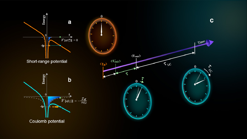
Refer to caption — Figure 1: Fig.1 $\mid$ Electron tunnelling and tunnelling delay time. The tunnelling of an electron is illustrated in the case of a, short-range potential and b, Coulomb potential. The white dashed lines in a and b are the field-free short-range and Coulomb potential, respectively. The blue shadows denote the nonzero potential interaction region during the tunnelling. c, The time components constitute the measured angular offset. $\tau_{LC}$ is the time induced by the Coulomb interaction in the continuum. See the main text for $\langle{t_{0}}\rangle$ , $\langle{t^{\prime}_{exit}}\rangle$ , $\langle{t_{exit}}\rangle$ and $\tau$ .

In a recent work on the hydrogen atom, to eliminate the Coulomb interaction in the continuum, a short-range potential instead of atomic potential was adopted in the numerical solution of the time-dependent Schrödinger equation (TDSE), which leads to an angular offset of zero and the argument of instantaneous electron tunnelling [10]. However, this substitution not only eliminated the Coulomb interaction in the continuum, but also diminished the sub-barrier potential interaction during the tunnelling, because the short-range potential rapidly approaches $0$ within the barrier region (see the white dashed curve in Figs. 1a and 1b). This would inevitably alter the sub-barrier potential interaction and the time a tunnelling particle spends inside the potential barrier, i.e. the tunnelling time.

Here, we perform energy-resolved electron attosecond angular streaking measurements (see S1 in Supplementary Information, SI) on Xe for comparison with velocity-dependent atom Larmor clock measurements [11]. The photoelectron momentum distribution (PMD) of tunnelling electrons driven by a 40 fs laser pulse presents a series of above-threshold ionization (ATI) rings spaced by one-photon energy [20, 21]. The ATI rings exhibit different most probable angular offsets, which offer a unique way to explore the energy-dependence of electron tunnelling (Fig. 2a). The energy-resolved measurements are reproduced by the numerical solution of a three-dimensional TDSE. The simulated and experimental results reach quantitative agreement (Figs. 2d-h).

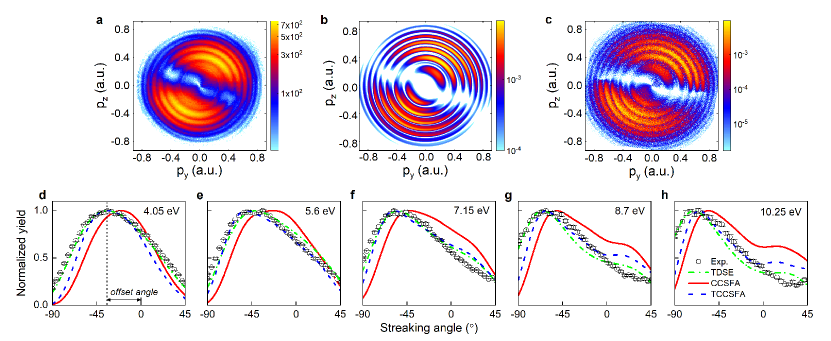
To highlight the importance of sub-barrier potential interaction in the classically forbidden region, we first provide a consistent tunnelling-Coulomb-corrected strong-field approximation (TCCSFA, details in S2 of SI) method which fully includes the potential interactions both during and after tunnelling, and then compare the simulation results with that when the sub-barrier potential interaction is neglected. It has been thought previously that the sub-barrier potential interaction during the tunnelling hardly changes the final PMD [22], however, here we clarify that it actually plays an essential role on the more accurate energy-resolved attoclock experiment: only when the sub-barrier potential interaction is taken into account, the simulations can quantitatively reproduce the angular offsets in both the experiment and TDSE calculations for different energies (blue dashed lines in Figs. 2d-h), otherwise, the angular offsets are obviously smaller (red solid lines in Figs. 2d-h). These results explicitly demonstrate that the sub-barrier potential interaction during tunnelling indeed takes time, which can be measurable via the energy-resolved attoclock measurements.

The TCCSFA method is based on the Feynman path integral (FPI), in which the probability amplitude of a quantum wave function can be represented as a coherent superposition of contributions of all possible spatio-temporal paths [23, 24]. Tunnelling is a typical nonclassical process where an electron spends imaginary time within the barrier, $t_{s}=t_{r}+\emph{i}t_{i}$ [25]. The real part of $t_{s}$ is the ionization time, i.e. the moment when an electron exits the barrier along a certain sub-barrier path, $t_{exit}=t_{r}=\textbf{Re}{(t_{s})}$ , and the imaginary part is related to the weight of the electron along this path. Since each path is deterministic, we can trace back exactly the ionization time and the probability of the electron along paths contributing to any part of the final PMD we are interested in [7, 18, 26].

Figure 3a shows the evolution of the electron wave packet (EWP) contributing to the third ATI ring during the tunnelling in the classical forbidden region. For each complex path, the ionization time is constant, while the weight changes during the evolution along the imaginary time. Here, the ionization time $t_{r}$ can be at any time, but the probability might be different. This reflects the probability wave nature of a tunnelling electron, where the behaviour is no longer deterministic and causal. In practice, we can explore the statistical average of the ionization time by evaluating all the involved complex paths: $\langle{t_{r}}\rangle=\frac{\sum_{i}W(i)\cdot t_{r}(i)}{\sum_{i}W(i)}$ [27, 28], where $W(i)$ is the weight of each path $i$ .

The green solid line in Fig. 3a shows the statistical averaged ionization time during the imaginary time evolution from $t_{s}$ until $t_{exit}$ , i.e., $t_{i}=0$ . It oscillates around the peak of the laser field during the tunnelling. At the tunnelling exit, the statistical averaged ionization time $t_{exit}>0$ . This oscillatory behaviour can be seen more clearly in Fig. 3b where we zoom into the region around $t_{r}=0$ . For comparison, we also show the case where all the potential interactions are neglected (the dashed black line). In this case, its ionization time equals $0$ during the imaginary time evolution without any oscillation, indicating instantaneous tunnelling. Similar rules can be found for other ATI rings.

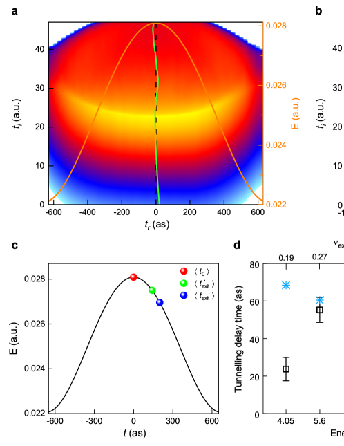
Figure 4: tunnelling is included (green dot), and the Coulomb interaction both during and after the tunnelling are considered (blue dot) in the tunnelling. d, Black squares denote the reconstructed tunnelling delay times from different ATI peaks, and the upper axis shows their corresponding velocities at the tunnelling exit. The light blue stars represent the Keldysh tunnelling time, and the dashed yellow line indicates the velocity matching the effective height of the barrier. The error bars show the standard deviation of statistical errors for reconstructing the tunnelling time from multiple sampling in a range of 8 degrees centred around the most probable angles for each ATI ring.

Then, the following question arises: dose the nonzero statistical averaged ionization time at the tunnelling exit correspond exactly to the tunnelling time, i.e. the time of sub-barrier potential interaction? According to the assumptions in conventional strategies of reconstructing tunneling time[19], the answer would be ’yes’, because only the tunnelling process could determine the ionization time according to the causality. However, surprisingly, we find that the statistical averaged ionization time of the paths contributing to the highest signal in the PMD is nonzero even when only the Coulomb interaction in the continuum is considered (the green dot in Fig. 3c). This ionization time is slightly smaller than that in TCCSFA simulation but it is obviously larger than that in the case where all the potential interactions are neglected, namely, time 0 (the blue and red dot in Fig. 3c).

In attoclock measurements, the angular offset is measured according to the highest photoelectron signal in the final PMD, which was assumed to be emitted at the peak of the electric field. However, over twenty years ago, Landauer et al. claimed that measuring the tunnelling time by following the peak should ’deserves least attention’, because they have noticed that an incident peak of EWP would not turn into a transmitted peak, particularly in the present of strong deformations [29, 30]. Here, the deformation results from the Coulomb interaction. When Coulomb deformation is completely neglected, the EWP behaves as a plane wave. In this case, an incident peak of the EWP at the tunnelling exit indeed turns into the most probable distribution in the final PMD (black dashed lines in Figs. 3a and 3b, and the red dot in Fig. 3c). However, the outgoing EWP would be divergent owing to the Coulomb interaction in the continuum. Both the final momentum and the phase of each path would be different compared to the case without Coulomb interaction. Owing to the quantum interference, the highest signal in the PMD would arise from a complete different set of paths, where statistical averaged ionization time would be delayed relative to that in the plane wave case (the red dot in Fig. 3c), which means that the Coulomb interaction in the continuum can induce ionization time delay. Obviously, this delay has no correlation with the tunnelling process but is due to the properties of electron wavepacket in the continuum. Hence, only when both wave and particle properties are fully taken into account, the tunnelling dynamics encoded in the attoclock measurements can be fully understood.

The electron tunnelling in the experiment contains potential interactions both within the barrier and in the continuum, and the statistical averaged ionization time of the quantum paths contributing to the most probable signals in PMD is further delayed (the blue dot in Fig. 3c). This additional ionization time delay corresponds to the time of the sub-barrier potential interaction. Close inspection reveals that the impact of the sub-barrier potential interaction on the quantum paths is different with that of Coulomb interaction in the continuum. We find that the sub-barrier potential interaction mainly changes the imaginary part $t_{i}$ of quantum path but keeps the real part $t_{r}$ nearly unchanged, which means that it does not slow down the electron along a certain sub-barrier path, but changes the probability of electron along this path, altering the evolution of the entire tunnelling EWP.

According to the statement of Landuer et al. [30, 29], following the highest probability signals is the largest drawback inherent in the attoclock measurements. However, this does not mean that attoclock cannot be used to measure the electron tunnelling time. The key point lies in that one should extract the ionization time delay solely induced by the sub-barrier potential interaction. Here, with the wave-particle duality in mind, and based on the fact that the measured energy-resolved most probable angular distribution can be quantitatively reproduced using the TCCSFA simulation, we propose that the tunnelling delay time can be constructed using the relative ionization time delay between the measurement and the case that neglecting the sub-barrier potential interaction during the tunnelling, i.e. $\tau=\langle t_{exit}\rangle-\langle t_{exit}^{\prime}\rangle$ , where $\langle t_{exit}\rangle$ is the corresponding statistical averaged ionization time in the measurement, and $\langle t_{exit}^{\prime}\rangle$ is the statistical averaged ionization time in the case without the sub-barrier potential interaction during the tunnelling (sketched in Fig. 1c).

Figure 3d shows the extracted tunnelling delay time, which ranges from $24$ to $58$ attosecond for ATI rings of different energies. Interestingly, this energy-dependent trend of the extracted tunnelling delay time of the electron is consistent with that in the measurements of atom tunnelling [11]. Above the effective barrier height, the trend is in agreement with the improved classical quasi-static model of Keldysh time (see details in the S3), i.e. an electron with higher velocity spends less time during the tunnelling (see the light blue stars in Fig. 3d). Below the effective barrier height, the counterintuitive phenomenon observed in atom tunnelling is also confirmed, i.e. a slower electron with a lower energy has a shorter tunnelling time [11].

In summary, the tunnelling delay time, i.e., the time of sub-barrier potential interaction, can be explicitly extracted by embracing the wave-particle duality. Our results not only unify the tunnelling time of atoms and electrons but also gain a deep insight into the tunnelling dynamics of matter waves. Manipulating the sub-barrier potential interaction would provide an unprecedented opportunity to control the tunnelling dynamics in microsystems, which could be used in applications such as manufacturing sub-nanoscale quantum devices at Moore’s limit, speeding up enzymatic catalysis, and preventing spontaneous mutations in DNA [33, 34, 35, 31, 32].

References

[1] Maccoll, L. A. Note on the transmission and reflection of wave packets by potential barriers. Phys. Rev. 40, 621-626 (1932).
[2] Hartman, T. E. Tunneling of a wave packet. J. App. Phys. 33, 3427-3433 (1962).
[3] Büttiker, M. Larmor precession and the traversal time for tunneling. Phys. Rev. B 27, 6178-6188 (1983).
[4] Spielmann, Ch., Szipöcs, R., Stingl, A. & Krausz, F. Tunneling of optical pulses through photonic band gaps. Phys. Rev. Lett. 73, 2308-2311 (1994).
[5] Steinberg, A. M. How much time does a tunneling particle spend in the barrier region? Phys. Rev. Lett. 74, 2405-2409 (1995).
[6] Balcou, Ph. & Dutriaux, L. Dual optical tunneling times in frustrated total internal reflection. Phys. Rev. Lett. 78, 851-854 (1997).
[7] Landsman, A. S. et al. Ultrafast resolution of tunneling delay time. Optica 1, 343-349 (2014).
[8] Torlina, L. et al. Interpreting attoclock measurements of tunnelling times. Nat. Phys. 11, 503-508 (2015).
[9] Camus, N. et al. Experimental evidence for quantum tunneling time. Phys. Rev. Lett. 119, 023201 (2017).
[10] Sainadh, U. S. et al. Attosecond angular streaking and tunnelling time in atomic hydrogen. Nature 568, 75-77 (2019).
[11] Ramos, R., Spierings, D., Racicot, I. & Steinberg, A. M. Measurement of the time spent by a tunnelling atom within the barrier region. Nature 583, 529-532 (2020).
[12] Eckle, P. et al. Attosecond ionization and tunneling delay time measurements in helium. Science 322, 1525 (2008).
[13] Schultze, M. et al. Delay in photoemission. Science 328, 1658 (2010).
[14] Paul, P. M. et al. Observation of a train of attosecond pulses from high harmonic generation. Science 292, 1689 (2001).
[15] Goulielmakis, E. et al. Real-time observation of valence electron motion. Nature 466, 739-743 (2010).
[16] Shafir, D. et al. Resolving the time when an electron exits a tunnelling barrier. Nature 485, 343-346 (2012).
[17] Orlando, G., McDonald, C. R., Protik, N. H., Vampa, G. & Brabec, T. Tunnelling time, what does it mean? J. Phys. B 47, 204002 (2014).
[18] Hofmann, C., Landsman, A. S. & Keller, U. Attoclock revisited on electron tunnelling time. J. Mod. Opt. 66, 1052-1070 (2019).
[19] Pazourek, R., Nagele, S. & Burgdörfer, J. Attosecond chronoscopy of photoemission. Rev. Mod. Phys. 87, 765-802 (2015).
[20] Agostini, P., Fabre, F., Mainfray, G., Petite, G. & Rahman, N. K. Free-free transitions following six-photon ionization of xenon atoms. Phys. Rev. Lett. 42, 1127-1130 (1979).
[21] Wang, C. et al. Accurate in situ measurement of ellipticity based on subcycle ionization dynamics. Phys. Rev. Lett. 122, 013203 (2019).
[22] Huismans, Y. et al. Time-resolved holography with photoelectrons. Science 331, 61-64 (2011).
[23] Feynman, R. P. Space-time approach to non-relativistic quantum mechanics. Rev. Mod. Phys. 20, 367-387 (1948).
[24] Feynman, R. P. & Hibbs, A. R. in Quantum mechanics and path integrals. Emended by Styer, D. F. (McGraw Hill, New York, 2005).
[25] Popov, V. S. Imaginary-time method in quantum mechanics and field theory. Phys. At. Nucl. 68, 686-708 (2005).
[26] Landsman, A. S. & Keller, U. Attosecond science and the tunnelling time problem. Phys. Rep. 547, 1-24 (2015).
[27] Sokolovski, D. & Baskin, L. M. Traversal time in quantum scattering. Phys. Rev. A 36, 4604-4611 (1987).
[28] Fertig, H. A. Traversal-time distribution and the uncertainty principle in quantum tunneling. Phys. Rev. Lett. 65, 2321-2324 (1990).
[29] Landauer, R. & Martin, T. Barrier interaction time in tunneling. Rev. Mod. Phys. 66, 217-228 (1994).
[30] Büttiker, M. & Landauer, R. Traversal time for tunneling. Phys. Rev. Lett. 49, 1739-1742 (1982).
[31] Löwdin, P.-O. Proton tunneling in DNA and its biological implications. Rev. Mod. Phys. 35, 724-732 (1963).
[32] Zhu, X. L. et al. Heavy N⁺ ion transfer in doubly charged N₂Ar van der Walls cluster. Nat. Commun. 11, 2987 (2020).
[33] Tong, J. et al. Tunnelling of electrons via the neighboring atom. Submitted.
[34] Godbeer, A. D., Al-Khalili, J. S. & Stevenson, P. D. Modelling proton tunnelling in the adenine-thymine base pair. Phys. Chem. Chem. Phys. 17, 13034-13044 (2015).
[35] Ball, P. Quantum biology. Nature 474, 272-274 (2011).

{addendum}

This work was supported by the National Natural Science Foundation of China (Grant Nos. 91950101, 11627807, 11774130, 11774215, 12074240 and 12004133) and the National Basic Research Program of China (No. 2019YFA0307700), DD and XL acknowledge the support of Science Challenge Project (TZ2018005), and WFY and XHS acknowledge the support of the Department of Education of Guangdong Province (Grant No. 2018KCXTD011) and the Mobility Programme of the Sino-German Center (Grant No. M-0031).

DD and CW conceived the experiments. XL, CW and YY conducted the measurements, CW, WY, XS, XL and SZ interpreted the results, XL prepared the figures. XL, JL, XS, JC and WY provided the calculations. CW, XL, XS, WY and DD prepared the manuscript. All authors reviewed the manuscript.

The authors declare that they have no competing financial interests.

Correspondence and requests for materials should be addressed to Chuncheng Wang (ccwang@jlu.edu.cn), Xiaohong Song (songxh@stu.edu.cn), Weifeng Yang (wfyang@stu.edu.cn), or Dajun Ding (dajund@jlu.edu.cn).