Zeus: Efficiently Localizing Actions in Videos using Reinforcement Learning

Abstract.

Detection and localization of actions in videos is an important problem in practice. State-of-the-art video analytics systems are unable to efficiently and effectively answer such action queries because actions often involve a complex interaction between objects and are spread across a sequence of frames; detecting and localizing them requires computationally expensive deep neural networks. It is also important to consider the entire sequence of frames to answer the query effectively.

In this paper, we present Zeus, a video analytics system tailored for answering action queries. We present a novel technique for efficiently answering these queries using deep reinforcement learning. Zeus trains a reinforcement learning agent that learns to adaptively modify the input video segments that are subsequently sent to an action classification network. The agent alters the input segments along three dimensions - sampling rate, segment length, and resolution. To meet the user-specified accuracy target, Zeus’s query optimizer trains the agent based on an accuracy-aware, aggregate reward function. Evaluation on three diverse video datasets shows that Zeus outperforms state-of-the-art frame- and window-based filtering techniques by up to 22.1$\times$ and 4.7$\times$, respectively. It also consistently meets the user-specified accuracy target across all queries.

1. Introduction

Recent advances in video database management systems (VDBMSs) (Kang et al., 2019; Lu et al., 2018; Bastani et al., 2020) have enabled automated analysis of videos at scale. These systems have primarily focused on retrieving frames that contain an object of interest. We instead are interested in detection and localization of actions in long, untrimmed videos (Shou et al., 2016; Xia and Zhan, 2020; Chao et al., 2018). For example, as shown in Figure 1, an action refers to an event spread across a sequence of frames. A traffic analyst might be interested in studying the patterns in which vehicles move at a given intersection. They might want to identify the density of pedestrian crossing in a particular direction.

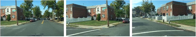
Figure 1. Sequence of frames capturing a car taking a left turn. None of the individual frames are sufficient to independently determine and localize the action. State-of-the-art frame-level techniques tailored for object detection are unable to answer action queries.

Action Localization Task. Action localization involves locating the start and end point of an action in a video, and classifying those frames into one of the available action classes (e.g., ‘left turn of a car’). Processing action queries requires the detection and localization of all occurrences of a given action in the video. The following query retrieves all the video segments (i.e., a contiguous sequence of frames) that contain a left turn of a car with 80% accuracy:

⬇

--- Retrieve segments with a left turn action

SELECT segment_ids FROM UDF(video)

WHERE action_class = ’left-turn’

AND accuracy >= 80%

In this query, $segment\_id$ is a unique identifier for each segment in the video with a start and end frame; $accuracy$ is the user-specified target accuracy for the query. The UDF is a user-defined function that returns predictions for each segment including the action class (e.g., turn) and the action boundary (list of segments).

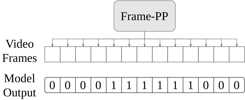
(a) Frame-PP approach

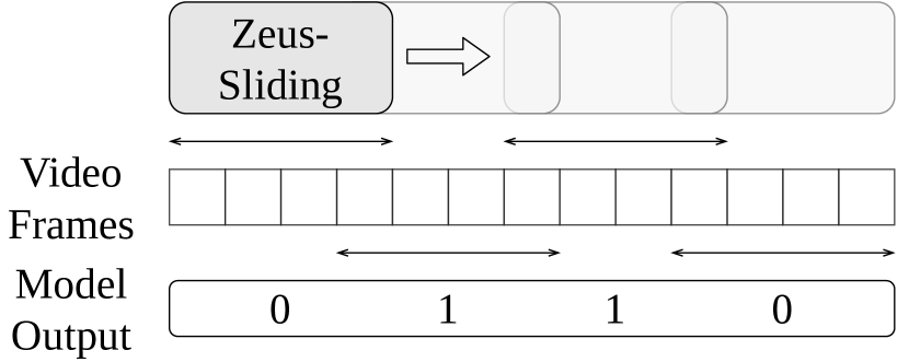
(b) Zeus-Sliding approach

Figure 2. Frame- and window-based techniques for action localization in videos.

Frame-based filtering. Recent VDBMSs primarily focused on accelerating content-based object detection queries in videos (Kang et al., 2017; Kang et al., 2019; Lu et al., 2018). They rely on quickly filtering frames that are not likely to satisfy the query’s predicate using different proxy models. The VDBMS may use this frame-based filtering technique to process action queries by filtering frames in the video that do not satisfy the action predicate. We refer to this technique as frame-level probabilistic predicate (abbrev., Frame-PP (Lu et al., 2018)).  Figure 2(a) illustrates an example.

Window-based filtering. Recent solutions (Simonyan and Zisserman, 2014; Tran et al., 2018) take a fixed-length segment in the video as input and return a binary label indicating the presence or absence of an action. The input segments contain three knobs: (Resolution of each frame, Segment Length– number of frames in the segment, Sampling Rate– frequency at which each frame is sampled). We refer to these as a Configuration tuple. To process action queries, a naïve solution that the VDBMS could use is to apply the deep learning model in a sliding window fashion on the video to detect actions and localize action boundaries, as illustrated in Figure 2(b). The inputs to the model are video segments of a single fixed configuration. We refer to this baseline technique as Zeus-Sliding. Another approach is to extend the frame-based filtering techniques in (Kang et al., 2017; Kang et al., 2019; Lu et al., 2018) to segments and build proxy models that can quickly filter irrelevant segments. We refer to this baseline technique as Segment-PP.

Challenges. To efficiently process action queries, the VDBMS must handle three challenges:

I. Task Complexity. Actions involve a complex interaction between objects within a video segment. For example, the action Pole Vault comprises of: a person carrying a pole, running, and jumping over a hurdle using the pole. Notice how the action comprises of multiple entities, and an interaction between these agents in a specific manner. The VDBMS has to detect all such actions and localize the start/end of the actions. These queries must accurately capture the temporal context and the scene complexity; this is too difficult for Frame-PP and Segment-PP which apply lightweight frame- and segment- level filters.

II. Computational Complexity. Zeus-Sliding may localize complex actions using a deep neural network (e.g., R3D (Tran et al., 2018)). But these networks are computationally expensive. At a frame resolution of 720$\times$720, the R3D model runs at 2 frames per second (fps) on a 16-core CPU, or at 13 fps on a server-grade GPU. Further, both Frame-PP and Zeus-Sliding are sample inefficient - they require processing a large chunk of frames or (overlapping) video segments to achieve a desired accuracy.

III. Accuracy Targets. While processing action queries, it is important to satisfy the user-specified accuracy target, trading between accuracy and query performance. Frame-PP and Segment-PP struggle to reach the target accuracy due to their inability to capture the temporal context and scene complexity respectively. Consider the illustrative example in Figure 1. None of the individual frames is sufficient for Frame-PP to localize the action boundaries. Meanwhile, each Zeus-Sliding model provides only a single accuracy configuration throughout the video.

Our Approach. We present Zeus, a VDBMS designed for efficiently processing action queries. Unlike prior systems that rely on proxy models, Zeus takes a novel approach based on adaptive input segments. In particular, at each time step, it uses an Adaptive Proxy Feature Generator (APFG), a module that adaptively generates latent features of the video segment at a small cost, thus enabling (1) classification of the action class of the segment, and (2) choosing the next input segment to process from a large space of possible inputs. We refer to these intermediate features as ProxyFeatures. Zeus configures the input knobs when picking the next segment. By doing so, Zeus also quickly skims through the irrelevant parts of the video.

It is challenging to choose the optimal knob settings for deriving the next segment at each time step. Consider an agent that: (1) uses slower knob settings if the current segment is an action, and (2) uses faster knob settings otherwise. We refer to this baseline with hard-coded rules as Zeus-Heuristic. With this technique, the VDBMS efficiently skims through non-action frames. However, it does not have fine-grained control over the target accuracy, since the rules only indirectly affect accuracy. Consider the case where the action spans the entirety of the video. Zeus-Heuristic would process the entire video with slower knobs, even when the accuracy target allows faster processing with a few mispredictions. Further, Zeus-Heuristic does not scale well to multiple knob settings.

We formulate choosing the optimal input segments at each time step as a deep reinforcement learning (RL) problem (Mnih et al., 2013). During query planning, Zeus trains an RL agent that learns to pick the optimal knob settings at each time step using the proxy features. To meet the accuracy target, the query planner incorporates novel accuracy-aware aggregate rewards into the training process. The use of an RL agent enables Zeus to: (1) maintain fine-grained control over accuracy, (2) achieve higher query throughput over the other baselines by automatically using the optimal knob settings at each time step, and (3) scale well to multiple knobs. We provide a qualitative comparison of the techniques for processing action queries in  Table 1.

Sequence Adaptive Auto-Knob Accuracy Inputs Inputs Selection Targets Frame-PP Segment-PP ✓ Zeus-Sliding ✓ ✓ Zeus-Heuristic ✓ ✓ Zeus ✓ ✓ ✓ ✓

Table 1. Techniques for processing action queries. Zeus (1) operates on a sequence of frames at a time, (2) adaptively selects input segments to boost performance, (3) automatically chooses the knob settings, and (4) has fine-grained control over query accuracy.

Contributions. In summary, the key contributions are:

• We highlight the limitations of SOTA filtering techniques on action queries( § 1). We present a novel approach for circumventing these limitations by using proxy features generated by an adaptive action recognition model ( § 3).

• We develop a reinforcement learning-based query planner that trains an RL agent to dynamically choose the optimal input configurations for the action recognition model ( § 4).

• We propose an accuracy-aware aggregate reward for training the RL agent and meeting the user-specified accuracy target( § 4.5).

• We implement the RL-based query planner and query executor in Zeus. We evaluate Zeus on six action queries from three datasets and demonstrate that it significantly improves over state-of-the-art in terms of query processing, while consistently meeting the accuracy target ( § 6).

2. Background

Action queries focus on (1) action classification (Karpathy et al., 2014; Carreira and Zisserman, 2017; Tran et al., 2018) which answers what actions are present in a long, untrimmed video, and (2) temporal boundary localization (Shou et al., 2016; Chao et al., 2018) for where these actions are present in the video. We refer to the combined task of detecting, and localizing actions in videos as action localization (AL).

AL focuses on retrieving events in a video that happen over a span of time, and that often involve interaction between multiple objects. For example, a traffic analyst may be interested in examining video segments that contain pedestrians crossing the road from left to right (CrossRight) from a corpus of videos obtained from multiple cameras. This query requires detection of: (1) pedestrians in the frame, (2) walking action of the pedestrian, and (3) trajectory of the person (left to right). The VDBMS must also accurately detect the start and end of this action.

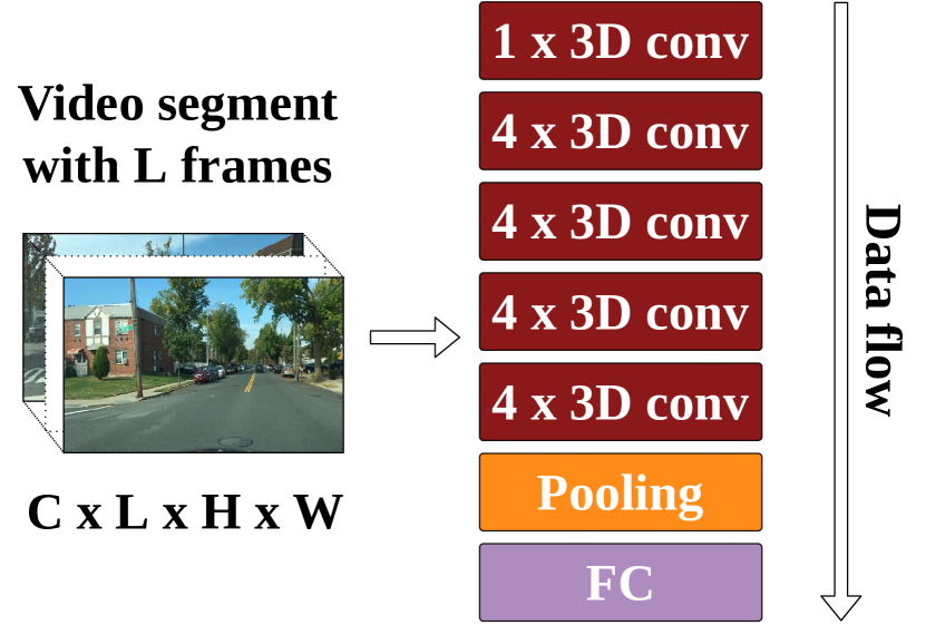
(a) 3D convolutions in R3D

Kernel	Output size
{3$\times$7$\times$7, 64} $\times$ 1	64 $\times$ L $\times$ H/2 $\times$ W/2
{3$\times$3$\times$3, 64} $\times$ 4	64 $\times$ L$\times$ H/2$\times$ W/2
{3$\times$3$\times$3, 128} $\times$ 4	128 $\times$ L/2 $\times$ H/4 $\times$ W/4
{3$\times$3$\times$3, 256} $\times$ 4	256 $\times$ L/4 $\times$ H/8 $\times$ W/8
{3$\times$3$\times$3, 512} $\times$ 4	512 $\times$ L/8 $\times$ H/16 $\times$ W/16
1$\times$1$\times$1	512 $\times$ 1
512 $\times$ $n\_classes$	$n\_classes$ $\times$1

(b) Data flow in R3D

Figure 3. The R3D network consists of 17 3D convolutional layers followed by adaptive average pooling and fully-connected layers. The input to the network is a video segment of length L frames. In successive 3D convolutional operations, the input is reduced to eventually get a 512 dimensional feature vector.

Neural Networks for AL. Researchers have proposed deep neural networks (DNNs) for AL. An early effort focused on using 2D convolutional neural networks (CNNs) to classify actions (Karpathy et al., 2014). 2D-CNNs are typically used for image classification and object detection and do not effectively capture information along the temporal domain (i.e., across frames in a segment). For the same reason, the frame-level filtering in recently proposed VDBMSs (Kang et al., 2017; Lu et al., 2018; Kang et al., 2019) is suboptimal for AL.

Frame-level filtering is also unable to accurately detect the action boundaries. This is because frames before, during, and after the scene of the action can be visually indistinguishable. In our evaluation section, we show that Frame-PP operates at prohibitively low accuracies for action queries (§ 6.2).

3D-CNNs for AL. 3D-CNNs (e.g., R3D (Tran et al., 2018)) apply the convolution operation along both spatial and temporal dimensions ( Figure 3(a)). This allows them to aggregate information along the temporal domain. More formally, consider an input video segment of size $C\times L\times H\times W$, where $C$ is the number of channels, $L$ is the number of frames in the segment, and $H$ and $W$ are the height and width of each frame. For each channel in $C$, the $L\times H\times W$ cuboid is convolved with a fixed size kernel to generate a 3D output. Outputs for each channel are pooled to produce a single 3D output in $L^{\prime}\times H^{\prime}\times W^{\prime}$ that corresponds to one kernel. With $K$ kernels, we obtain a $K\times L^{\prime}\times H^{\prime}\times W^{\prime}$ matrix as the output of each layer. The overall network consists of a series of such spatio-temporal 3D convolutional blocks.

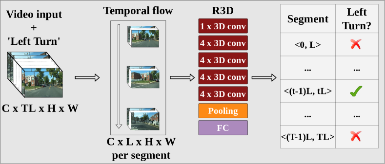
Figure 4. In Zeus-Sliding, the input video of T $\times$ L frames is divided into T segments of L frames each. Each segment is then processed by the R3D network to generate binary class labels to determine the presence/absence of action.

Zeus-Sliding. As demonstrated in Figure 4, the Zeus-Sliding technique (recall § 1) uses the R3D network in a sliding window fashion over the input video. For each segment of size $L$, all frames are stacked together to form a 4D input segment and are passed to the R3D network, which generates class labels for the current window; the VDBMS slides the window forward by a specified number of interval frames. In this manner, the network classifies and localizes the actions.

However, Zeus-Sliding is computationally expensive. The R3D model has significantly more parameters – 33.4 million which is 3$\times$ higher than the corresponding 2D resnet-18 model. On an NVIDIA GeForce RTX 2080 Ti GPU, at the resolution of 480x480, the R3D network processes 27 frames per second (fps), while its 2D counterpart processes frames at 156 fps. This limits current VDBMSs to analyse video data at scale.

2.1. Problem Formulation

Given an input video, the objective of our system, Zeus, is to efficiently process the video and find segments that contain an action. Each video may contain different types of actions. Given a label function $\mathbb{L}(n)$ that provides the oracle action label at frame $n$, the binary label function for an action class X is defined as:

(1) $$f_{\_}X(n)=\begin{cases}1&\text{if }\,{\mathbb{L}(n)=X}\\ 0&\text{if }\,{\mathbb{L}(n)\neq X}\end{cases}\quad$$

Zeus measures the accuracy of the query with respect to the oracle label function $\mathbb{L}(n)$. A binary ground truth label for a segment is generated using intersection-over-union (IoU) over the frame-level ground truth labels. A given segment of length K frames is labeled as a true positive if IoU¿0.5 over labels $\mathbb{L}(n)$ to $\mathbb{L}(n+K)$. Zeus compares the output of the classifier and the segment index against this segment label to compute the query accuracy. Zeus seeks to efficiently process this AL query while meeting the target accuracy, i.e., the accuracy target specified by the user with the query.

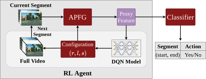
Figure 5. Architecture of query executor in Zeus– The query executor uses a deep RL agent to process action queries. It takes as input the ProxyFeature generated by the APFG, to output a Configuration, which is used to construct the next input segment. The ProxyFeature is also processed by a classifier to predict the presence of action in the current segment.

Time Step	t=1	t=2	t=3	t=4	t=5
Frame Number	f=1	f=65	f=97	f=101	f=113
Configuration	(150, 8, 8)	(200, 6, 4)	(300, 4, 1)	(250, 6, 2)	(150, 8, 8)
Segment	(1, 64)	(65, 96)	(97, 100)	(101, 112)	(113, 176)
APFG Prediction	NO-ACTION	ACTION	ACTION	ACTION	NO-ACTION

Figure 6. Illustration of Zeus on CrossRight action – At each time step, Zeus picks from a set of configurations to generate the next input to the APFG. Each Configuration is a 3-tuple (Resolution, Segment Length, Sampling Rate).

3. Executing Action Queries

Overview. We propose a system, Zeus, to efficiently answer AL queries. Figure 5 demonstrates the architecture of the query executor in Zeus with the following components:

• Segment: Each video segment is characterized by ¡start, end¿ which represent the start and end frames of the action. start, end $\in[1,N]$, where $N$ is the total number of frames.

• ProxyFeature: A fixed-size vector of floats that succinctly represents an input video segment.

• APFG: Denotes an Adaptive Proxy Feature Generator. It is a collection of action recognition models that adaptively generate ProxyFeatures based on the configuration (e.g., a collection of R3D models that operate on input segments of varying segment lengths and resolutions).

• Classifier: A model that emits the action label.

• Configuration $(r,l,s)$ - Concrete setting of three knobs - Resolution, Segment Length, and Sampling Rate (§ 1).

At a given time step t, Zeus takes a video segment of length $l_{\_}t$, resolution $r_{\_}t\rightarrow(h_{\_}t,w_{\_}t)$, sampled once every $s_{\_}t$ frames, to generate a 4D vector of size $3\times l_{\_}t\times h_{\_}t\times w_{\_}t$ as the input. The APFG module processes this input and generates a proxy feature vector $\hat{Z}_{\_}{t}$, which is then passed to a classification network that predicts the presence or absence of an action in the current segment. The RL agent also uses $\hat{Z}_{\_}{t}$ to generate the next Configuration $(r_{\_}{t+1},l_{\_}{t+1},s_{\_}{t+1})$, using which the APFG constructs the next segment of size $3\times l_{\_}{t+1}\times h_{\_}{t+1}\times w_{\_}{t+1}$ sampled at a frequency of $s_{\_}{t+1}$.

APFG. Unlike prior VDBMSs, Zeus relies on ProxyFeatures as opposed to a proxy model. In particular, it uses the APFG to generate the ProxyFeatures for the segments in the video. The APFG is an ensemble of action recognition models (e.g., R3D) that can adaptively process input segments of varying resolutions and segment lengths to generate the ProxyFeatures. More specifically, the ensemble contains models trained for different resolutions and segment lengths. Typically, models trained with one configuration have a lower accuracy when tested on other configurations. So, the ensemble design provides a better accuracy and flexibility compared to a single R3D model, that only supports segments of fixed resolution and length. Moreover, the APFG can leverage a wide range other of action recognition models. So, the R3D model can be easily replaced with better (faster, more accurate) models if necessary. Since training models for each configuration is expensive, we present an optimization to lower this cost in § 5.

Zeus processes the ProxyFeatures from APFG using a classification network to determine the presence or absence of actions. This technique allows Zeus to infer complex relationships present in the scene. Besides classifying the given scene, Zeus uses the ProxyFeature to also construct the next input to the APFG. In particular, it trains a deep RL agent to tune the configuration with 3 knobs. The agent learns to use segments of low-resolution, coarse-grained sampling (fast Configuration) for portions of the video that are unlikely to contain an action. Otherwise, it uses high-resolution, fine-grained sampling (slow Configuration).

Illustrative example. Consider the example shown in Figure 6. Zeus localizes a CrossRight action (i.e., a pedestrian crossing the street from left to right).

At time step $t=1$, Zeus starts at frame number 1. Assume Zeus has access to a ProxyFeature $\hat{Z}_{\_}{0}$ from the previous time step. Since there is no CrossRight in this segment, Zeus uses a low resolution $150\times 150$, high segment length $(8)$ and high sampling rate $(8)$ to construct the input to the APFG. Henceforth, the knob settings will be represented as a Configuration- $(150,8,8)$ in this case. We use the most accurate (and computationally expensive) configuration as this first configuration at time step 1. We only use square-shaped frames with equal height and width. The APFG processes the segment $(1,64)$ sampled once every 8 frames to generate a ProxyFeature $\hat{Z}_{\_}{1}$ and a prediction NO-ACTION. Thus, Zeus processes $8\times 8$ frames in this time step at a low resolution of $150$, jumping to the frame $65$. At $t=2$, Zeus processes the ProxyFeature $\hat{Z}_{\_}{1}$ from $t=1$. Since $\hat{Z}_{\_}{1}$ aggregates information for frames 1 to 64, the agent learns the possibility of CrossRight at the end of the segment (f = 64). So, Zeus uses a slower Configuration of $(250,6,4)$ to generate $\hat{Z}_{\_}{2}$ and the prediction ACTION. Notice that the Configuration change from $t=1$ to $t=2$ is gradual, since the possibility of CrossRight has not been fully established in $t=1$. At $t=3$, Zeus processes the ProxyFeature $\hat{Z}_{\_}{2}$, which was generated from a higher resolution finely-sampled input. So, Zeus recognizes the presence of an action and uses a slow Configuration of $(300,4,1)$ to generate $\hat{Z}_{\_}{3}$ and the prediction ACTION. At $t=4$, Zeus processes $\hat{Z}_{\_}{3}$ and generates the Configuration $(250,6,2)$. It slightly increases the Configuration speed since it recognizes that CrossRight may end soon at f=100. However, the prediction for this segment is still ACTION. Finally, at $t=5$, Zeus detects the end of CrossRight and reverts to the fastest Configuration of $(150,8,8)$.

Across five time steps, Zeus performs 5 invocations of the APFG, processes $176$ frames, with 160 of those frames processed at less than half of the highest resolution, while still accurately localizing the action boundaries from $(65,112)$. In this way, Zeus efficiently and accurately localizes and classifies the target action.

4. Planning Action Queries

We present the internals of the query planner in this section. We begin with a discussion on how we formulate the RL problem in § 4.1. We then describe how the query planner picks the configurations that can be used for processing a given query in § 4.2. In § 4.3, we present an overview of the RL algorithm used in Zeus. We then describe the local reward function in § 4.4. Since this function does not always meet the accuracy constraint, we discuss a reward aggregation strategy in § 4.5. Lastly, in § 4.6, we outline how the query planner trains an accuracy-aware RL agent.

4.1. RL Formulation

The goal of the agent is to choose configurations at each time step such that the overall query processing time is minimized while the target accuracy is satisfied (as discussed in § 3).

Heuristics vs RL. In theory, Zeus could leverage an agent that uses hard-coded rules to determine the parameters for constructing the segment. For example, consider the rule: if the video contains an ACTION at the current time step, then the agent should use a lower sampling rate. However, such a hard-coded low sampling rate is sub-optimal since the agent does not have fine-grained control over the query accuracy. In Figure 6, Zeus-Heuristic would use the slow Configuration $(300,4,1)$ at time step $t=3$ and get the ACTION signal from the APFG. So, Zeus-Heuristic again uses the slow configuration, and only processes 4 frames in time step $t=4$ as opposed to Zeus that processes 12 frames in time step $4$ (as shown in Figure 6). Zeus-Heuristic keeps using the slow configuration for time steps $5$, $6$, and $7$, since the prediction at each of these time-steps is ACTION. Effectively, Zeus-Heuristic reaches frame 112 only at time step $7$, while Zeus does so by time step $4$. This would be sub-optimal since the agent would process 16 frames in the sequence (97, 112) at a significantly lower throughput, while potentially overshooting the accuracy target. So, Zeus-Heuristic cannot trade-off the accuracy for throughput. Furthermore, the number of such rules will increase with the number of available configurations and may interact in unexpected ways (Haas et al., 1989).

To circumvent these problems, Zeus uses an RL-based agent that adaptively changes the segment’s parameters. For a given accuracy target, Zeus trains the RL agent to trade-off the excess accuracy for throughput improvement. We compare the performance of Zeus against Zeus-Heuristic in § 6.2.

Markov Decision Process. Most RL problems are modelled as Markov Decision Processes (MDP) (Howard, 1960; Shoham et al., 2003). An RL problem formulated as MDP is characterized by an agent that takes actions in an environment. Each action changes the state of the agent in the environment, and the agent receives a reward for its actions. We formulate our problem as an MDP with the following components:

• Environment: The set of training videos V {$v_{\_}1,v_{\_}2,\cdots,v_{\_}N$}.

• State: 4D tensor for the segment $(s,e)$.

• Reward: Reward function for training the agent (§ 4.4) that maps each step taken by the agent to a scalar reward value.

• Configuration: Configuration chosen by the agent at each time step from the set of available configurations $\{c_{\_}1,c_{\_}2,\cdots,c_{\_}n\}$.

Resolution Segment Length Sampling Rate Throughput (fps) F1-score 150 4 8 1282 0.57 200 4 4 553 0.82 250 6 2 285 0.86 300 6 1 115 0.91

Table 2. Illustrative list of configurations used by Zeus– Each configuration has associated throughput and accuracy metrics.

4.2. Configuration Planning

Given an input query with a target accuracy, the query planner seeks to maximize throughput while satisfying the accuracy constraint. To achieve this goal, it first collects the appropriate settings for all of the knobs for the given query (i.e., a Configuration). Each configuration has two associated cost metrics: (1) throughput (fps), and (2) accuracy. For example, using coarse-grained sampling leads to faster (but less accurate) query processing.

Pre-Processing. In a one-time pre-processing step during the query planning phase, Zeus computes the cost metrics associated with each configuration on a held-out validation dataset. It uses Zeus-Sliding (Figure 4) to compute these metrics. Table 2 lists a few configurations for the CrossRight query after this step. Notice that the throughput and the accuracy of the configurations is inversely proportional. This pattern allows the VDBMS to trade-off throughput and accuracy by choosing faster configurations if the accuracy is greater than the accuracy target.

4.3. Deep Q-Learning

Input : Query Q, Number of training episodes = T

Set of N training videos V = {$v_{\_}1,v_{\_}2,\cdots,v_{\_}N$}

Output : Trained DQN-Network $\phi$

Initialize :  Ground_Truths(GT); APFG(U);

Replay_Buffer(B); DQN_Network($\phi$);

1 for i $\leftarrow 1$ to T do

       // Initialize episode

2       V_i, GT_i $\leftarrow$ Random_Order(V, GT);

3       segment_curr $\leftarrow$ Init_Segment(V_i);

4       state_curr $\leftarrow$ U(segment_curr);

5       while $idx$(segment_curr) ¡ size(V) do

             // Generate experiences

6             config_curr $\leftarrow$ argmax($\phi$(segment_curr));

7             reward, segment_next $\leftarrow$ TraverseVideo(V_i, GT_i, config_curr);

8             state_next $\leftarrow$ U(segment_next, config_curr);

             // push experience to replay buffer

9             B.push(state_curr, config_curr, reward, state_next);

             // Update DQN model

10             if $update_{\_}{\phi}$ then

11                   minibatch $\leftarrow$ B.sample(batchsize);

12                   qvalues, targets $\leftarrow$ $\phi$(minibatch);

13                   loss $\leftarrow$ HuberLoss(qvalues, targets);

14                   update_weights($\phi$, loss);

15                  

16             state_curr $\leftarrow$ state_next;

17             segment_curr $\leftarrow$ segment_next;

18            

Algorithm 1 Algorithm for training the RL agent

We now provide an overview of the RL algorithm used in Zeus. Deep Q-learning (DQN) is a variant of the Q-learning algorithm for RL (Mnih et al., 2013). The original Q-learning algorithm takes numerical states as inputs and uses a memoization table (called the Q-table) to learn the mapping of a given state to a particular configuration. In DQN, this mapping is learnt by a DNN that approximates the Q-table. DQN works well when the state space of the inputs and/or the configuration space is large. Since visual data is high dimensional, DQN is often used to train RL agents that operate on images or videos (e.g., Atari games).

Training Process. Algorithm 1 outlines the DQN technique used by Zeus to train an RL agent for action queries. The training algorithm assumes the presence of ground truth labels, and trained APFG. The DQN algorithm has two main components: (1) the agent collects experiences by traversing through the video (Algorithm 1 to Algorithm 1), and (2) it updates the model parameters (model’s mapping of the video and configurations) using the collected experiences (Algorithm 1 to Algorithm 1). To generate a new experience, the agent applies the configuration config_curr output by the network (Algorithm 1) to transition from the current state state_curr to the next state state_next in the video (Algorithm 1 to Algorithm 1). The agent receives a reward for this transition (Algorithm 1) (§ 4.4). This 4-tuple of (state_curr, config_curr, reward, state_next) is called an experience tuple. The agent continuously collects new experience tuples by traversing through the video, and updates the model parameters periodically to account for the newly observed experience tuples.

One way to achieve this behavior is to always use the most recently generated experience tuples to update the Q-network. However, such tuples are from nearby segments in the video and hence highly correlated. DNN training process is known to be ineffective when learning with correlated tuples. To overcome this problem, DQN uses an experience replay buffer. This is a cyclic memory buffer that stores the experience tuples from the last K transitions (a hyperparameter). While generating experiences, the agent pushes the new experience tuples to the replay buffer (Algorithm 1). During the update step of DQN, Zeus samples a mini-batch of experiences from the replay buffer (Algorithm 1) and updates the model parameters (Algorithm 1). This technique improves the model’s sample efficiency by reducing the correlation between samples during a single update step.

Convergence Speed. DQN is notoriously slow to converge on large state spaces (Mnih et al., 2013). It requires a large number of experience tuples to approximate the Q-value function. This problem is more significant for video segment inputs since experience generation is slower with 4D tensors. Additionally, the replay buffer size is prohibitively large when the states are raw 4D tensors. Thus, representing states using raw 4D tensors is impractical even on server-grade GPUs. To circumvent this problem, Zeus first generates the video segment segment_next during the transition (Algorithm 1). The APFG then processes segment_next to generate the proxy features that serve as the next state state_next of the agent (Algorithm 1). The APFG is trained independently of the RL agent and its weights are frozen during the RL training process. This ProxyFeature is then used as the state for the RL agent.

4.4. Local Reward Allocation

The agent’s goal is to select a Configuration at each time step that minimizes query processing time while satisfying the accuracy requirement. To minimize processing time, the agent should skip more frames and pick lower resolutions. To meet the accuracy requirement, the agent should use high resolution and fine-grained sampling in the vicinity of action segments within the video.

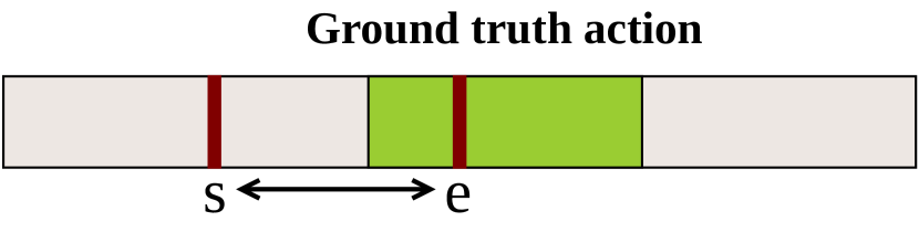
(a) Penalty

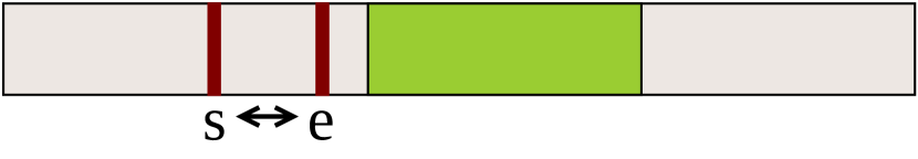
(b) Low reward

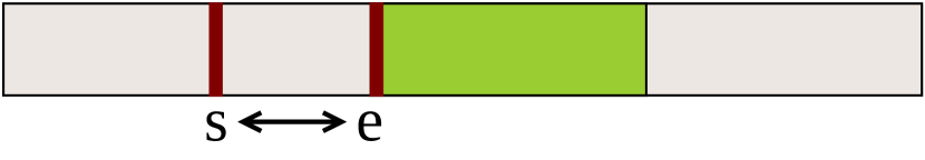
(c) High reward

Figure 7. Reward Scenarios – The reward function (§ 4.4) assigns reward to the agent differently for each of the scenarios shown above.

Local Reward Function. To achieve these goals, one way to model the reward function (Algorithm 1 in Algorithm 1) for the agent would be: (1) reward decisions that increase the processing speed, and (2) penalize decisions that lower accuracy. At a given time step $t$, let us assume that the agent outputs the Configuration- $(r,l,s)$. With this configuration, the segment window that is processed in this time step is $(s,e)\rightarrow(f_{\_}{curr},f_{\_}{curr}+s*l)$, where $f_{\_}{curr}$ is the current location of the agent. Lets assume that each configuration $c$ has an associated scalar value $\alpha_{\_}{c}$ that represents the fastness of a configuration (i.e., throughput in Table 2). The faster the configuration, the greater the value of $\alpha_{\_}{c}$. The $\alpha$ values are further normalized such that $\sum_{\_}{c=1}^{N}\alpha_{\_}{c}=1$, where $N$ is the number of available configurations. Then, the reward function can be formulated as:

(2) $$r_{\_}t(s,e)=\begin{cases}\beta-\alpha_{\_}{curr}&\text{if }\exists i\in[s,e):\mathbb{L}_{\_}A(i)=1\\ \alpha_{\_}{curr}&\text{if }\forall i\in[s,e):\mathbb{L}_{\_}A(i)=0,\\ \end{cases}\quad$$

where $\mathbb{L}_{\_}A(i)$ is the label function (§ 2.1), and $\beta$ is cutoff that divides the configuration space into fast and slow configurations.

The intuition behind this function is that for action frames ($\mathbb{L}_{\_}A(i)=1$), the reward should be inversely proportional to the fastness $\alpha$ since we desire slower more accurate configs. Conversely, for non-action frames ($\mathbb{L}_{\_}A(i)=0$), the reward should be proportional to $\alpha$. Thus, the function only looks at the local ground truth values to assign the reward. With this reward function, the agent checks for the existence of ground truth frames in the local segment window $(s,e)$. If there is an action frame in this window (Figure 7(a)), the agent penalizes configurations that are fast (low resolution, coarsely-sampled) and rewards slow configurations.

On the other hand, if there is no action frame in this window, the agent rewards fast configurations. For example, in Figure 7(b), the reward assigned to the decision is positive, but has a low value. This is because the agent does not utilize the full window available before the start of the action. In contrast, the decision in Figure 7(c) receives the maximum reward. Notice that the agent does not penalize slow configurations when there is no action in this window. This design prioritizes the reduction of false negatives over performance.

This technique does not have explicit control over the query accuracy, similar to the Zeus-Heuristic approach. However, it scales well with multiple knob settings since it is automated.

4.5. Aggregate Reward Allocation

Algorithm 1 trains the agent to accelerate the query while penalizing any decision that leads to missing action frames (Figure 7(a)). So, the agent optimizes for reducing false negatives (instead of performance). This often leads to a much higher accuracy than the target at reduced throughput. So, the query planner can further lower execution time using this excess accuracy budget.

Baseline. To satisfy the accuracy constraint, Zeus-Sliding picks the configuration that is closest to the target accuracy (i.e., just above the required accuracy) for all the segments. However, this approach is sub-optimal. To achieve an aggregate accuracy of 80% with a better throughput, the agent may pick configurations with 90% and 70% expected accuracy for video segments that contain and that do not contain actions, respectively. Since actions are typically infrequent in videos, this strategy leads to higher throughput by using the faster configuration most of the time, and occasionally using the slower, more accurate configuration. Thus, the query planner must take the accuracy constraint into consideration during the training process to obtain maximum performance.

Reward aggregation. The RL agent must learn the optimal strategy for picking configurations across the video to minimize query execution time within the given accuracy budget. To tackle this problem, the query planner uses an accuracy-aware aggregate reward allocation strategy. Here, the query planner accumulates the agent’s decisions during a predetermined window $W$. During this accumulation phase, the algorithm does not immediately assign a reward to the agent. Specifically, in Algorithm 1 of Algorithm 1, the agent only receives a reward after it processes all the frames in $W$. At the end of the window, the aggregate accuracy of the agent’s decisions is evaluated. Based on the actual and target accuracy metrics, it computes the reward for all the local decisions taken within this window. We use the term aggregate to emphasize that we do not immediately assign local rewards as in Equation 2. We instead accumulate decisions during each window, then compute the reward for this window (shown in § 4.6), and finally assign the (same) reward to all the decisions in the window.

Input : Video V, Target Accuracy $\alpha$, Window W $\rightarrow(s,e)$

$C\rightarrow\{c_{\_}1,c_{\_}2,\cdots,c_{\_}k\}$

Binary frame-wise ground truths GT(W) of size $|e-s|$

Trained APFG U

Output : List of size k with scalar rewards for each decision in C

Initialize :  Pred(W) $\leftarrow$ Empty list of size $|e-s|$;

1 Procedure GetReward(V, $\alpha$, C)

       // Collect predictions

2       for i $\leftarrow$ $1$ to k do

3             segment $\leftarrow$ GetSegment(V, c_i);

4             pred(i) $\leftarrow$ U(segment, c_i);

5             Update_Prediction_List(pred(i));

6            

7       $\alpha\prime\leftarrow$ Accuracy(GT(W), Pred(W));

       // Assign rewards

8       if $\alpha^{\prime}\geq\alpha$ then

9             $r_{\_}i\leftarrow\frac{1-\alpha^{\prime}}{1-\alpha}\forall i\in[1,k]$;

10            

11       else

12             $r_{\_}i\leftarrow\alpha^{\prime}-\alpha\forall i\in[1,k]$;

13            

14      

Algorithm 2 Accuracy-Aware Reward Assignment Algorithm

4.6. Global Accuracy-Aware Rewards

As discussed in § 4.5, local rewards are not sufficient to ensure that Zeus efficiently meets the global target accuracy constraint. Hence, we modify the reward function used in Algorithm 1 (Algorithm 1) to use the aggregate accuracy metric presented in § 4.5. Algorithm 2 outlines how the query planner computes the accuracy-aware aggregate reward at the end of each window W. Assume that the agent takes $k$ steps in this window, then $\{c_{\_}1,c_{\_}2,\cdots,c_{\_}k\}$ is the sequence of configurations chose by the agent in the $k$ time steps. With the aggregate window approach, the query planner first collects predictions in the window (Algorithm 2 to Algorithm 2). Next, it computes the overall accuracy in the window using ground truth labels (Algorithm 2). The query planner then assigns a reward to all the decisions in the window based on the accuracy achieved by the agent.

Updated reward function. Algorithm 2 to Algorithm 2 show the updated accuracy-based reward function. If the target accuracy $\alpha$ is met within the window, the query planner assigns a reward that increases when the achieved accuracy is closest to the target accuracy (Algorithm 2). The intuition behind this reward is that, as long as the accuracy achieved is greater than the target accuracy, we want to maximize the throughput. As we have seen in Table 2, the throughput is maximum when the accuracy is minimum. When the gap between achieved and target accuracy is as small as possible, the achieved accuracy is minimized, as long as it is above the target. So, the throughput is maximized while respecting the accuracy constraint. For example, if the accuracy within the window exceeds target accuracy, the query planner assigns a low reward, ensuring that the agent tries to exploit this excess accuracy. Conversely, if the accuracy in the window is less than the target accuracy, the query planner assigns a penalty (negative reward) that is directly proportional to the accuracy deficit (Algorithm 2). So, the lower the accuracy of the agent, the greater the penalty.

To compute aggregate rewards, query planner uses a delayed replay buffer update strategy to collect experiences. During the processing of the current aggregation window, query planner uses Algorithm 1 to collect the incomplete experience tuples (without reward) into a temporary buffer. At the end of each window, the agent updates the experience tuples in the temporary buffer with the rewards collected using Algorithm 2. Zeus then pushes the updated experience tuples to the replay buffer. With these modifications to Algorithm 1, Zeus achieves a higher throughput than Zeus-Sliding, while also meeting the accuracy target.

Accuracy Guarantees. Since Zeus combines different configurations of R3D (§ 4.2), the final accuracy achieved is dependent on the accuracy achieved by the R3D model with individual configurations (Table 2). Zeus utilizes accurate configurations for action frames and less accurate configurations for non-action frames. Thus, Zeus ensures a high recall in the output at the cost of slightly lower precision. For a given accuracy target, the reward function in Zeus balances the precision and recall such that the resultant F1-score is closest to the target. On the other hand, Zeus-Sliding is the only other baseline that reaches the accuracy target, since we manually select such configuration from the configuration planning phase § 4.2. Zeus-Heuristic cannot reliably reach the accuracy target since the rules do not provide explicit control over the accuracy.

Like state-of-the-art baselines (Kang et al., 2019; Kang et al., 2017; Lu et al., 2018), approximate ML inference queries cannot guarantee accuracy on unseen test data. So, all the baselines (including Zeus-Sliding) cannot be guaranteed to reach the accuracy target on unseen data. However, we empirically show that Zeus meets the target accuracy (e.g., target=75-85% in § 6.2 and § 6.3) when test and train data distributions are similar, while other baselines often fail to do so. We further show that Zeus maintains its throughput gains over other methods when trained on one dataset and tested on a different dataset (§ 6.6) with a slight accuracy drop in all the methods (including Zeus-Sliding) due to the variations in data distribution.

5. Implementation

APFG Training. Recall from § 3 that the objective of the APFG is: (1) to predict the action class labels, and (2) to generate features for a given input segment. Zeus trains the APFG using the segments extracted from a set of training videos along with their binary labels (i.e., whether a particular action class is present or absent in the segment). It adopts a fine-tuning strategy to train the APFG to accelerate the training process. Specifically, it uses the pre-trained weights of the R3D model trained on the Kinetics-400 dataset (Carreira and Zisserman, 2017) and fine-tunes the parameters for the target action classes. We add three fully-connected layers to the original R3D model.

Model reuse. Recall that the APFG is a collection of action recognition models that can processing varying resolutions and segment lengths. We optimize the APFG training process by approximating the ensemble of models with a single R3D model. That is, we use one R3D model with the highest accuracy to generate ProxyFeatures for all configurations. The intuition behind this design is that the model trained on the most accurate configuration (i.e., with the highest resolution and lowest sampling rate) can also process faster configurations (e.g., lower resolutions), albeit at a slight accuracy drop. Note that the alternative, i.e., re-training the model on lower resolution configurations would also incur an accuracy drop due to the low resolution, and would significantly increase the training time. Although the empirically observed accuracy for the latter strategy is slightly higher, the former approach leads to much lower training times. Since the APFG allows model flexibility, assuming that the computational resources are available, one could also train the models individually for the configurations.

RL Training. To train the RL agent, Zeus use the DQN algorithm with an experience replay buffer. We configure the replay buffer to 10 K experience tuples and initialize it with 5 K tuples. Zeus’s DQN model is a Multi-layer Perceptron (MLP) with 3 fully-connected layers. We use a batch size of 1 K tuples to train the DQN model. We concatenate all the individual training videos to create episodes of equal time span. This ensures that the agent receives similar rewards during each episode. This design decision is critical to optimize the behavior of the RL agent over time. Additionally, Zeus permutes the videos in a random order for each episode to prevent overfitting to the specific order in which the RL agent processes the videos.

Pre-Processing. RL training typically takes more time to converge compared to supervised deep learning algorithms. This is because of the large number of experience tuples required for training the Q-network. To accelerate this training process, Zeus first runs the APFG on all the input segments at different resolutions and segment lengths to generate the feature vectors. This preprocessing step uses a batching optimization and leverages multiple GPUs to lower the RL training time significantly. The agent then directly uses the precomputed features during training.

Software Packages. We implement Zeus in Python 3.8. We use the PyTorch deep learning library (v 1.6) to train and execute the neural networks. Zeus uses the R3D-18 model with pre-trained weights from the PyTorch’s TorchVision library (tor, [n.d.]), and fine-tunes it to the evaluation datasets (§ 6.1). The weights of the APFG are frozen during the subsequent RL training process. We use the OpenAI Gym (v 0.10.8) library for simulating the RL environment (Brockman et al., 2016).

6. Evaluation

In our evaluation, we illustrate that:

• Zeus executes queries up to 4.7$\times$ faster than the state-of-the-art baseline (Zeus-Sliding) at a given target accuracy (§ 6.2), 8.3$\times$ higher throughput and $0.25$ points higher F1 score on average compared to existing VDBMSs (Frame-PP) (§ 6.2), with a maximum speedup of 22.1$\times$.

• Zeus consistently achieves the user-specified accuracy target at a better throughput than other baselines (§ 6.3). Meanwhile, Zeus’s knobs contribute to the throughput increase (§ 6.4).

• The RL agent in Zeus is practical – a single model can be trained to detect multiple similar actions (§ 6.5) and the same model can detect a given action in multiple datasets (§ 6.6).

• Zeus’s query planner incurs only a small overhead for training the RL agent (§ 6.7) and leveraging available configurations for performance improvement (§ 6.8).

Dataset No. of Total Percent Avg. Action Std. (Min, Max) classes Frames (K) Actions length Dev. Length BDD100K 2 $186$ 7.03 115 58.7 (6, 305) Thumos14 2 $645$ 40.27 211 186.3 (18, 3543) ActivityNet 2 $633$ 56.37 909 1239.1 (20, 6931)

Table 3. Dataset Characteristics – We report these key characteristics of the datasets we evaluate Zeus on: (1) number of action classes and total frames, (2) average percentage of action frames across all frames, (3) average and standard deviation of length of action instances, and (4) length of shortest and longest action instances.

6.1. Experimental setup

Evaluation queries and dataset. We evaluate Zeus on six queries from three different action localization datasets. For the first four queries, we use publicly available datasets: Thumos14 (Jiang et al., 2014) and ActivityNet (Caba Heilbron et al., 2015). Each has hundreds of long, untrimmed videos collected from several sources. We take two classes from each dataset to construct four action queries -

• Thumos14 - PoleVault, CleanAndJerk

• ActivityNet - IroningClothes, TennisServe

However, these datasets contain high density of actions (i.e., more than 40% of the video frames contain actions) (see Table 3). To better study the impact of action length and percentage of action frames (abbrev., action percentage), we leverage a novel dataset tailored for evaluating action analytics algorithms. This dataset consists of a subset of 200 videos from the BDD100K (Berkeley Deep Drive) dataset (Yu et al., 2020). Each video is $\approx$ 40 seconds long, collected at 30 fps, and contains dash-cam footage from cars driving in urban locations. We manually annotate these videos with two action classes/queries:

• CrossRight: In this query, the pedestrian crosses the street from the left side of the road to the right side (Figure 6).

• LeftTurn: This query returns the segments in the video that contain a left turn action the driver’s point-of-view.

Dataset Characteristics. Table 3 lists the key characteristics of the datasets. The datasets vary significantly in action percentage and average action length. ActivityNet has the highest action percentage, and the action length varies significantly across videos (high std. deviation). BDD100K has shorter actions and lower action percentage (only 7% of all the frames are action frames).

Configurations. We list the available knob settings for each dataset in Table 4. Each unique combination of knob settings represents a candidate configuration. BDD100K dataset has a total of 64 available configurations (4$\times$4$\times$4), while Thumos14 and ActivityNet each has 27. Notice that the available segment lengths (window size) are longer for queries with higher action length and percentage. This results in a higher overall throughput for the datasets/queries with large action lengths/percentages (§ 6.2). On the contrary, we pick shorter segment lengths for BDD100K, since the action length and percentage is significantly smaller (Table 3). When the action length is shorter, the accuracy drops at larger window sizes. For example, if we use the configurations for ActivityNet (in table 4) on BDD100K, the accuracy drops rapidly because the configurations with large windows just completely skip the action.

Table 4 also lists the highest accuracy achieved by any configuration for each query. This denotes the upper bound on accuracy achievable by any of the query processing techniques for the query. The best accuracy is higher for BDD100K compared to Thumos14 and ActivityNet datasets. This is likely because: (1) BDD100K has relatively simple classes (e.g., left turn vs tennis serve), (2) It has higher resolution videos (300x300 vs 160x160), and (3) videos are collected from the same camera and environment.

Dataset Available Available Available Maximum Resolutions Segment Lengths Sampling Rates Accuracy BDD100K 150, 200, 250, 300 2, 4, 6, 8 1, 2, 4, 8 Cross Right 0.91 Left Turn 0.89 Thumos14 40, 80, 160 32, 48, 64 2, 4, 8 Pole Vault 0.78 Clean And Jerk 0.76 ActivityNet 40, 80, 160 32, 48, 64 2, 4, 8 Ironing clothes 0.85 Tennis serve 0.80

Table 4. Configuration Statistics – We report these statistics for each dataset we evaluate Zeus on: (1) Number of available resolutions to choose from, (2) Number of available segment lengths, (3) Number of available sampling rates, and (4) Maximum accuracy achieved by any configuration for a given query.

Hardware Setup. We conduct the experiments on a server with one NVIDIA GeForce RTX 2080 Ti GPU and 16 Intel CPU cores. The system is equipped with 384 GB of RAM. We use four GPUs for training and extracting features. We constrain the number of GPUs used during inference to one to ensure a fair comparison.

Baselines. We compare Zeus against three baselines.

• Frame-PP uses a 2D-CNN on individual frames in the video (2(a)) and outputs a binary label that determines the presence or absence of an action in that frame. Existing VDBMSs (Kang et al., 2017; Lu et al., 2018; Kang et al., 2019) use Frame-PP as a filtering optimization to accelerate object queries. To improve accuracy on action queries, we instead apply Frame-PP on all frames.

• Segment-PP uses a lightweight 3D-CNN filter on all non-overlapping segments in the video to quickly eliminate segments that do not satisfy the query predicate. The R3D model then processes the filtered segments to generate the final query output. Segment-PP extends the frame-level filtering optimization used in existing VDBMSs (Kang et al., 2017; Lu et al., 2018; Kang et al., 2019) to segments.

• Zeus-Sliding processes segments in the video using a 3D-CNN, specifically, the R3D network (Ji et al., 2013; Tran et al., 2018). We use the network in a sliding window fashion (2(b)) on the input video to generate segment-level predictions. Zeus-Sliding uses a static Configuration for the entire dataset. It chooses the fastest configuration that meets the target accuracy.

• Zeus-Heuristic dynamically uses a subset of available configurations based on hard-coded rules to process the video, including (1) using the slowest configuration when the APFG returns ACTION prediction, (2) a faster configuration when the APFG prediction flips from ACTION to NO-ACTION, and (3) the fastest configuration when the APFG returns a NO-ACTION prediction across ten consecutive time steps.

• We refer to the RL-based approach as Zeus-RL.

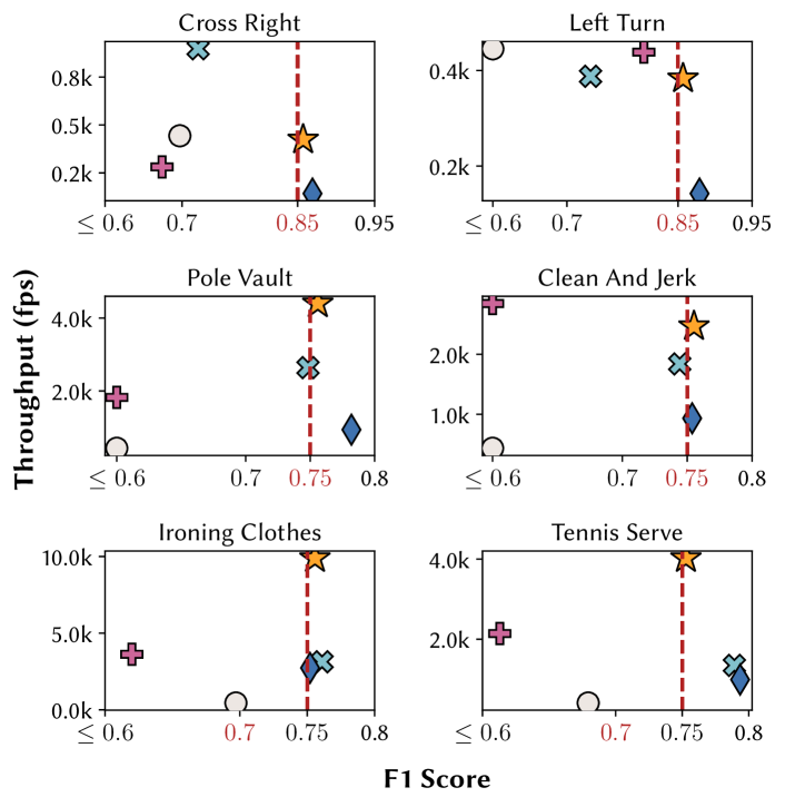
Figure 8. Throughput and F1 score achieved by Zeus-RL, Frame-PP, Segment-PP, Zeus-Heuristic, and Zeus-Sliding over Q1-Q6 (Top-right corner is best). Note that ranges are different for each query. The red dotted line represents the accuracy target set for each query.

6.2. End-to-end Comparison

We first compare the end-to-end throughput and accuracy metrics of Zeus-RL against the other baselines. We use accuracy target of $0.75$ for queries based on Thumos14 and ActivityNet, while $0.85$ for queries based on BDD100K (due to the maximum accuracy that can be achieved Table 4). In this experiment, Frame-PP uses the most accurate trained model (and hence with the highest available resolution). Zeus-Sliding uses the fastest configuration that achieves the accuracy target on training data. Zeus-Heuristic applies hard-coded heuristics on a subset of configurations that are used by Zeus-RL to process the query.

Zeus-Sliding. The results are shown in Figure 8. The red dotted line indicates the accuracy target for each query. Notably, on average, Zeus-RL is $3.4\times$ faster than Zeus-Sliding at a given target accuracy, with a maximum speed-up of $4.7\times$ in PoleVault. Zeus-RL outperforms Zeus-Sliding across all queries at the target accuracy. This shows that the additional configurations available to Zeus-RL help in improving performance. Zeus-Sliding is the only other baseline that reaches the accuracy target for all the queries. However, the accuracy achieved is often higher than the target (e.g., Tennis serve). In most cases, Zeus-RL achieves accuracy closest to the target accuracy. It efficiently uses the excess accuracy to improve throughput by using faster configurations, thus outperforming Zeus-Sliding.

Zeus-Heuristic. For four out of the six queries, Zeus-RL has a higher throughput than Zeus-Heuristic. The throughput delivered by Zeus-Heuristic is inversely proportional to the percentage of actions in the input videos. Consider the CrossRight (low percentage) and TennisServe (high percentage) queries. Zeus-Heuristic returns a low throughput in TennisServe and a high throughput in CrossRight (albeit at a lower accuracy). The reason for this behavior is that the hard-coded rules in Zeus-Heuristic state that the agent must pick the slower configurations for ACTION frames. So, Zeus-Heuristic does not have explicit control over query accuracy. When the fraction of action frames in the input video is high (e.g., TennisServe), Zeus-Heuristic uses slower configurations for majority of the frames in the video. So, it delivers a lower throughput while overshooting the accuracy target.

On the contrary, Zeus-RL does not have hard-coded rules. The RL agent is trained to automatically pick configurations that improve throughput while barely exceeding the accuracy target. This also explains why Zeus-Heuristic has a high throughput for CrossRight. This query contains fewer, shorter action segments, resulting in Zeus-Heuristic choosing the faster configurations most of the time, thereby skipping important frames (due to large window sizes). We show the concrete distribution of these configurations in § 6.8. Finally, Zeus-Heuristic performs better than Zeus-Sliding across most queries. This illustrates that dynamically selecting the configuration is better than using a static configuration. To summarize, (1) an RL-based agent is more efficient at selecting the optimal configuration at each time step than a rule-based agent, (2) dynamic configuration selection is better than a static configuration.

Segment-PP. Segment-PP returns a prohibitively low F1 score ($\leq 0.6$) for four out of the six queries. It returns a low accuracy for the harder action classes from the Thumos14 and ActivityNet datasets. This behavior can be attributed to the inability of the lightweight filters in Segment-PP to capture the inherent complexity of actions. On the other hand, notice that Segment-PP provides a better accuracy on the easier LeftTurn class. The throughput achieved by Segment-PP is a function of the action percentage in the videos. When action class is trivial and rare (e.g., LeftTurn), Segment-PP can rapidly eliminate segments that do not satisfy the predicate, thus providing a slightly better throughput. However, when the action classes are hard, the lightweight filters in Segment-PP are highly inaccurate (with F1 score as low as 0.2). In case of hard and rare classes (e.g., CrossRight), this results in increased false negatives and false positives, thus leading to a much lower F1 score and slightly lower throughput. Finally, when the action classes are hard and frequent (e.g., IroningClothes), the increased false negatives and false positives lead to both, a much lower throughput and accuracy than Zeus.

Frame-PP. Zeus-RL is $8.3\times$ faster and delivers $0.25$ points higher F1 score on average compared to Frame-PP. Zeus-RL uses segment-level processing to process up to 64 frames with a single APFG invocation. On the other hand, Frame-PP has to process each frame separately. So, even though each APFG invocation is 5.9$\times$ faster in Frame-PP (§ 2), the overall throughput of Zeus-RL is significantly higher. Inspite of processing each individual frame, Frame-PP still has a prohibitively low F1 score for all the queries. This is because these queries require a sequence of frames (temporal information) to predict the action class, and hence cannot be handled by Frame-PP.

Impact of Action Length and Action Percentage. The relative throughput of all the methods varies across datasets. We attribute this to variability in action length and action percentage across datasets (Table 3). The average speedup of Zeus-RL over Zeus-Sliding is the highest for ActivityNet (3.8$\times$) and lowest for BDD100K (2.8$\times$). So, Zeus-RL performs better when the action length and percentage are higher. For dataset with longer action sequences, we set a larger segment length and sampling rate (Table 4) for more efficient processing. So, each APFG invocation results in larger processed windows, resulting in proportionally larger absolute and relative throughput.

Figure 9. Performance and throughput of Zeus-Sliding and Zeus-RL over a range of target accuracies.

CrossRight LeftTurn Accuracy Accuracy Speedup Accuracy Accuracy Speedup Target Achieved Target Achieved 0.75 0.753 1.45 0.75 0.755 1.64 0.80 0.819 1.78 0.80 0.824 1.70 0.85 0.857 2.97 0.85 0.879 2.69

Table 5. Speedup of Zeus-RL over Zeus-Sliding over a range of accuracy targets

6.3. Accuracy-Aware Query Planning

In this experiment, we verify the ability of the query planner to generate an accuracy-aware query plan. Figure 9 shows the throughput vs accuracy curve for Zeus-RL and Zeus-Sliding at three accuracy targets over two queries. The red dotted line indicates the three different accuracy targets for the queries (0.75, 0.80, 0.85). Zeus-RL performs better than Zeus-Sliding over all the accuracy targets. Furthermore, Zeus-RL accuracy is consistently closer to the target accuracy, while Zeus-Sliding often overshoots this target. Zeus-RL efficiently allocates this excess accuracy budget by using faster configurations in certain segments to improve throughput, while ensuring that the accuracy is just over the target.

Table 5 shows the speedup of Zeus-RL over Zeus-Sliding at each accuracy target. The speedup is inversely proportional to the accuracy target. Recall that Zeus-RL uses the ProxyFeatures generated by the APFG to select the next configuration. When the accuracy target is low, the configurations available to Zeus-RL are all of low accuracy. So, Zeus-RL receives noisy features from the APFG, resulting in sub-optimal configuration selection.

6.4. Knob Selection

We investigate the contribution of different optimizations (i.e., knobs) to the throughput of Zeus-RL. Specifically, we disable each knob (fix the value) one at a time and examine its impact on throughput. The results are shown in Figure 10. Notably, all of the knobs contribute to the performance improvement, and Segment Length, Sampling Rate are the key knobs.

Across all queries, on average, disabling the Sampling Rate, the Segment Length, and the Resolution knobs reduces throughput by 62%, 51%, and 36% respectively. Note that the Sampling Rate and Segment Length knobs operate in tandem to determine the throughput of Zeus-RL. For example, when Segment Length is 8 and Sampling Rate is 8, the agent processes 64 frames in one time step. In contrast, when Segment Length is 2 and Sampling Rate is 1, it only processes 2 frames in one time step.

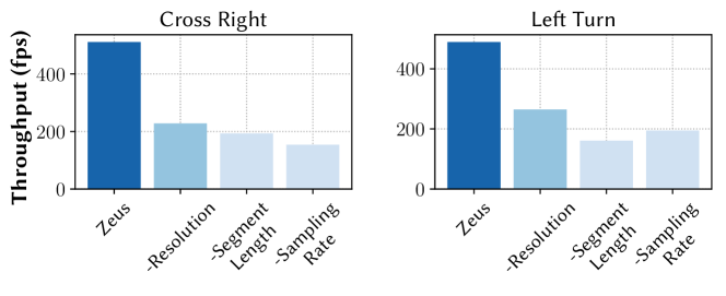
Figure 10. Impact of Resolution, Segment Length, and Sampling Rate knobs on the throughput of Zeus-RL. We disable each knob to study its impact on the overall throughput.

Importance of Knobs. We now examine why the Sampling Rate and the Segment Length knobs are important. The throughput of Zeus-RL is determined by two factors: (1) number of APFG invocations, and (2) time taken for each APFG invocation. Among these factors, the first one is more important. When Zeus-RL processes 10 frames using one APFG invocation (i.e., Segment Length = 10), it is 2$\times$ faster than using 5 APFG invocations (i.e., Segment Length = 2). The Sampling Rate and the Segment Length knobs reduce the number of APFG invocations, thereby improving throughput. The Segment Length knob determines the size of the input along the temporal dimension. A longer segment leads to higher APFG invocation time. So, the impact of this knob is comparatively smaller than that of the Sampling Rate knob. The impact of the Resolution knob is the least since it only affects the APFG invocation time.

APFG Invocation Time. We attribute the lower impact of each APFG invocation time to the lack of input batching. Since the RL agent is able to generate the next input only after processing the current input, it cannot exploit the batching capabilities of the GPU. So, Zeus-RL does not support intra-video parallelism. But, it is possible to extend Zeus-RL to support inter-video parallelism. Here, batching inputs across videos would allow better GPU utilization.

6.5. Practicality of Zeus

Figure 11. Multi-Class Training – Throughput and F1 curve for different methods trained on multiple classes together.

In this section, we study the practical applicability of Zeus.
Multi-class training. Since training one single RL agent for each action class may not be viable, we first examine the ability of Zeus to train on multiple classes together. More precisely, we combine the ground truths of the two action classes such that frames belonging to either of the action class are considered true positives and frames that belong to neither are considered true negative. Once the models return the output segments for both the classes, we can trivially separate them using another classifier since the output segments are only 3-4% of the full videos. We show the results in Figure 11. Most notably, Zeus-RL provides the best accuracy-performance trade-off even when trained on two classes. The performance of all the methods, specifically accuracy, is slightly better for the combination of (CrossRight, CrossLeft) compared to (CrossRight, LeftTurn). In the first case, the action instances are similar looking, thus lowering the task complexity. In the second case, the actions CrossRight and LeftTurn are characteristically different, which reduces the accuracy of the APFG and thus Zeus-RL. This also explains the high accuracy achieved by Frame-PP for the (CrossRight, CrossLeft) combination. When these classes are combined, the goal of Frame-PP reduces to detecting frames that contain a person in front of the car, making it a simpler task than detecting the walking direction of the person.

(a) Throughput and F1 score of model trained
on CrossRight

(b) Number of frames processed at each resolution when using the same model for both classes

Figure 12. Cross-Model Inference – Evaluation of model trained on CrossRight over other classes

Cross-model inference. In the second experiment, we use the RL agent trained on one class directly for other classes. More precisely, the RL agent takes decisions based on the features received from the APFG models. Our intuition is that the feature vectors generated by the APFG for different action classes are similar, especially for similar looking classes such as CrossRight and CrossLeft. So, we can directly use the RL agent trained for one action class on the other action class, just by using the APFG models corresponding to each class. To this end, we train an RL agent on the CrossRight class and directly use it for the CrossLeft and LeftTurn classes. We show the results in Figure 12(a). We can see that the model trained on CrossRight provides a decent throughput at minimal accuracy loss on the CrossLeft query. In fact, the model achieves a 2.2$\times$ speedup over the Zeus-Sliding baseline for the CrossLeft query. The throughput and accuracy are slightly lower when the same model is used for the LeftTurn class, since the differences in the action instances lead to more diverging feature vectors than those that the model is trained on. Finally, we show the number of frames processed at each resolution in Figure 12(b). When the CrossRight model is used directly for CrossLeft, we see that the number of frames processed at the high resolution of 300x300 increases, while those processed at 200x200 decreases. The slightly different feature vectors lead to some suboptimal decisions by the RL agent, but the overall trend still remains the same.

6.6. Domain Adaptation

In this experiment, we evaluate the domain adaptation ability of Zeus-RL. Specifically, we train Zeus-RL and the four baselines on the BDD100K driving dataset and run the trained models on the Cityscapes (Cordts2016Cityscapes) and the KITTI (Geiger2013IJRR) datasets. BDD100k dataset contains driving scenes from the streets of 4 US cities, while the Cityscapes dataset contains driving scenes from the city streets of Frankfurt, Germany. The KITTI dataset contains driving scenes from the residential streets of Karlsruhe, Germany. So, the datasets are inherently different in terms of scene composition and action distribution. We use the same experimental setup as § 6.2 with an accuracy target of $0.85$ for both queries. We evaluate the CrossRight query only on Cityscapes due to no available action instances for this class in the KITTI dataset. The results are shown in Figure 13.

Most notably, Zeus-RL maintains its advantages over the other baselines even when tested on different datasets. The relative performance of the different baselines remains consistent on the other datasets. All the methods fail to reach the accuracy target by a small margin ($\sim$2.5%). The slight accuracy drop is reasonable considering the challenges of tackling data drift (Suprem et al., 2020). The accuracy drop is more considerable in CrossRight than LeftTurn since the former is a more complex action. Similarly, the accuracy drop for LeftTurn is more significant in the KITTI dataset compared to the Cityscapes dataset since the residential scenes in KITTI lead to more variations in driving and action patterns. Zeus-RL provides accuracy on par with the most accurate approach i.e., Zeus-Sliding and does so at a better performance. Zeus-Heuristic suffers a significant accuracy drop in CrossRight and a throughput drop in LeftTurn. The inability of Zeus-Heuristic to balance accuracy and throughput is worsened on the other datasets (compared to  Figure 8) because individual decisions of the APFG are slightly less accurate, leading to higher noise in the efficacy of the rules. Frame-PP and Segment-PP achieve the lowest accuracy (as low as 0.15) when tested on the other datasets. Their inability to capture the complexities of actions is exacerbated when tested on unseen datasets.

Figure 13. Domain Adaptation – Throughput and F1 score of Zeus-RL and other baselines trained on the BDD100k dataset and evaluated on the Cityscapes and KITTI datasets.

6.7. Training Cost

We now examine the training overhead for Zeus-RL. We show the cost of training different components of the pipeline in Table 6. The APFG Training cost shown is the cost to train the 2D/3D-CNNs. Recall that we train the APFG only once with the best configuration (i.e., the highest resolution lowest sampling rate configuration) (§ 5). In the cost estimation phase (§ 4.2), we run the APFG (using Zeus-Sliding technique) with each configuration on a tiny held out validation set to get the throughput and accuracy of each configuration. Since this preprocessing cost is same for all the techniques, we omit it from the training cost.

The overall training time of Zeus-RL is 35% (90 sec) more than Zeus-Sliding, for training the RL agent. This is a one-time preprocessing cost for a given query and accuracy target. Further, the total training and inference time for Zeus-Sliding is still 27% higher than Zeus-RL owing to the faster inference with Zeus-RL. Finally, even though the training time of Zeus-Heuristic is comparable to Zeus-Sliding, Zeus-Heuristic needs manual construction of rules involving several configurations. This limits the practical applicability of Zeus-Heuristic.

Method APFG Training (s) RL Training (s) Inference (s) Frame-PP 101.81 NA 396.85 Zeus-Sliding 247.57 NA 181.06 Zeus-Heuristic 247.57 NA 64.21 Zeus-RL 247.57 90.00 38.52

Table 6. Training costs – We report the cost of: 1) Training the APFG 2) Training the RL agent 3) Inference

6.8. Configuration Distribution

We next examine the efficacy of Zeus-RL in choosing the appropriate configurations during query processing. The configurations differ in both their throughput and accuracy of processing queries (Table 2). We constrain the agent to use three configurations: (1) fast (but less accurate), (2) mid, and (3) slow (but more accurate). The experimental settings are same as § 6.2. We compare the percentage of frames processed using these configurations for Zeus-Heuristic and Zeus-RL. The results are shown in Figure 14(a).

Zeus-RL processes the videos using a combination of the configurations across all queries. This differs from Zeus-Heuristic that often uses a single configuration for most of the frames. On average, Zeus-Heuristic processes 85% of the frames using a single configuration. In Figure 14(a), notice that Zeus-Heuristic uses the fast configuration for majority of frames in CrossRight, while using the slow configuration for majority of the frames in PoleVault and IroningClothes. Since action percentage is low in CrossRight, Zeus-Heuristic uses the fastest configuration for most of the frames, and in the process, skips important frames. As a result, Zeus-Heuristic falls well short (0.72) of the accuracy target (0.85). Conversely, in PoleVault and IroningClothes, Zeus-Heuristic reaches the target accuracy but loses throughput (2$\times$ lower than Zeus-RL) due to the use of slow configurations.

In contrast, Zeus-RL uses a combination of the configurations in all the 3 queries. It barely exceeds the target accuracy in both the queries and achieves a high throughput.

Resolution Split. We further divide the frames in Figure 14(a) into low and high resolution frames, based on the configuration used to process them. Figure 14(b) shows the percentage of frames processed at high and low resolutions for Zeus-Heuristic and Zeus-RL. Zeus-Heuristic uses a low resolution for majority of the frames in CrossRight, since it has a low action percentage. On the other hand, it uses a high resolution in PoleVault and IroningClothes, which have significantly higher action percentages. We attribute this behavior to the rigidity of the rules used by Zeus-Heuristic. Zeus-RL on the other hand uses low resolution for majority of the frames in all three queries, regardless of the action percentage in the videos. This shows that the RL agent optimizes the throughput more efficiently.

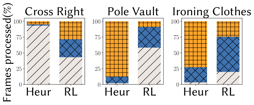
(a) Configuration distribution

Query Heuristic RL Cross Right 95/5 72/28 Pole Vault 12/88 91/9 Ironing Clothes 28/72 75/25

(b) Resolution (lo/hi(%))

Figure 14. (a) Percentage of frames processed by the fast, mid, and slow configurations for Zeus-Heuristic and Zeus-RL. (b) Percentage of frames processed at low and high resolutions in Zeus-Heuristic and Zeus-RL.

7. Related Work

Action Localization. Action Localization is a long-standing problem in computer vision. Early efforts in AL focused on feature engineering (e.g., SIFT (Lowe, 1999), HOG (Dalal and Triggs, 2005)), and hand crafted visual/temporal features (Xia and Zhan, 2020). To avoid hand-crafting features, deep neural networks have been proposed for AL. Two-stream networks (Simonyan and Zisserman, 2014; Feichtenhofer et al., 2016) use deep neural networks to process inputs in rgb stream and optical flow stream. 3D Residual Convolutional Neural Networks (3D-CNNs) (Tran et al., 2018) use 3D-convolutions to directly process 4D-input blocks (stacked frames). More recent work on AL includes SCNN (Shou et al., 2016), and TAL-Net (Chao et al., 2018). S-CNN and TAL-Net propose a three-stage approach for AL using proposal, classification, and localization networks. These above approaches focus on improving the accuracy of AL. On the other hand, Zeus focuses on improving throughput of AL queries while reaching a user-specified accuracy target.

Video Analytics. Recent advances in vision have led to the development of numerous VDBMSs for efficiently processing queries over videos. NoScope (Kang et al., 2017) uses a cost-based optimizer to construct a cascade of models (e.g., lightweight neural network and difference detector). Probabilistic Predicates (PP) (Lu et al., 2018) are lightweight filters that operate on frames to accelerate video classification. These lightweight models accelerate query execution by filtering out frames that do not satisfy the query predicate. BlazeIt (Kang et al., 2019) extends filtering to more complex queries (e.g., aggregates and cardinality-limited scrubbing queries). These lightweight filters accelerate execution by learning to directly answer the query instead of using a heavyweight deep neural network. These lightweight filter-based methods cannot capture complex temporal and scene information that is typically present in actions. MIRIS (Bastani et al., 2020) is a recently proposed VDBMS for processing object-track queries that requires processing a sequence of frames. It uses a graph neural network to keep track of objects between consecutive frames. It works well when a large number of frames satisfy the input query.

Zeus differs from these efforts in that it is tailored to optimize action queries while capturing the complex scene information. It trains an RL agent that adaptively chooses the input segments sent to the 3D-CNN. Thus, it operates on a sequences of frames, efficiently expresses complex scenes, and handles rare events.

RL for Video Processing. Researchers have applied RL for complex vision tasks such as video summarization (Zhou et al., 2018; Lan et al., 2018; Ramos et al., 2020). Deep Summarization Network (DSN) (Zhou et al., 2018) uses deep RL to generate diverse and representative video summaries. FastForwardNet (FFNet) (Lan et al., 2018) uses deep RL to automatically fast forward videos and construct video summaries on the fly. In contrast, Zeus uses RL to process action queries. Its optimizer leverages diverse knobs settings to reduce execution time.

8. Conclusion

Detecting and localizing actions in videos is an important problem in video analytics. Current VDBMSs that use frame-based techniques are unable to answer action queries since they do not extract context from a sequence of frames. Zeus processes action queries using a novel deep RL-based query executor. It automatically tunes three input knobs - resolution, segment length, and sampling rate - to accelerate query processing by up to 4.7$\times$ compared to state-of-the-art action localization techniques. Zeus uses an accuracy-aware query planner that generates aggregate rewards for training the RL agent, ensuring that the query executor achieves the user-specified target accuracy at a higher throughput than other baselines.

References

- (1)
- tor ([n.d.]) [n.d.]. PyTorch Torchvision. https://pytorch.org/vision/stable/index.html.
- tec ([n.d.]) [n.d.]. Zeus: Efficiently Localizing Actions in Videos using Reinforcement Learning. https://pchunduri6.github.io/files/chunduri2021zeus.pdf.
- Bastani et al. (2020) Favyen Bastani, Songtao He, Arjun Balasingam, Karthik Gopalakrishnan, Mohammad Alizadeh, Hari Balakrishnan, Michael Cafarella, Tim Kraska, and Sam Madden. 2020. MIRIS: Fast Object Track Queries in Video. In SIGMOD. 1907–1921.
- Brockman et al. (2016) Greg Brockman, Vicki Cheung, Ludwig Pettersson, Jonas Schneider, John Schulman, Jie Tang, and Wojciech Zaremba. 2016. OpenAI Gym. arXiv:1606.01540 [cs.LG]
- Caba Heilbron et al. (2015) Fabian Caba Heilbron, Victor Escorcia, Bernard Ghanem, and Juan Carlos Niebles. 2015. Activitynet: A large-scale video benchmark for human activity understanding. In CVPR. 961–970.
- Carreira and Zisserman (2017) Joao Carreira and Andrew Zisserman. 2017. Quo vadis, action recognition? a new model and the kinetics dataset. In CVPR. 6299–6308.
- Chao et al. (2018) Yu-Wei Chao, Sudheendra Vijayanarasimhan, Bryan Seybold, David A Ross, Jia Deng, and Rahul Sukthankar. 2018. Rethinking the faster r-cnn architecture for temporal action localization. In CVPR. 1130–1139.
- Dalal and Triggs (2005) Navneet Dalal and Bill Triggs. 2005. Histograms of oriented gradients for human detection. In CVPR, Vol. 1. Ieee, 886–893.
- Das et al. (2020) Nilaksh Das, Sanya Chaba, Renzhi Wu, Sakshi Gandhi, Duen Horng Chau, and Xu Chu. 2020. GOGGLES: Automatic Image Labeling with Affinity Coding. SIGMOD (May 2020). https://doi.org/10.1145/3318464.3380592
- Feichtenhofer et al. (2016) Christoph Feichtenhofer, Axel Pinz, and Andrew Zisserman. 2016. Convolutional two-stream network fusion for video action recognition. In CVPR. 1933–1941.
- Haas et al. (1989) L. M. Haas, J. C. Freytag, G. M. Lohman, and H. Pirahesh. 1989. Extensible Query Processing in Starburst. SIGMOD 18, 2 (June 1989), 377–388. https://doi.org/10.1145/66926.66962
- Howard (1960) Ronald A Howard. 1960. Dynamic programming and markov processes. (1960).
- Ji et al. (2013) S. Ji, W. Xu, M. Yang, and K. Yu. 2013. 3D Convolutional Neural Networks for Human Action Recognition. TPAMI 35, 1 (2013), 221–231. https://doi.org/10.1109/TPAMI.2012.59
- Jiang et al. (2014) Y.-G. Jiang, J. Liu, A. Roshan Zamir, G. Toderici, I. Laptev, M. Shah, and R. Sukthankar. 2014. THUMOS Challenge: Action Recognition with a Large Number of Classes. http://crcv.ucf.edu/THUMOS14/.
- Kang et al. (2019) Daniel Kang, Peter Bailis, and Matei Zaharia. 2019. BlazeIt: optimizing declarative aggregation and limit queries for neural network-based video analytics. VLDB 13, 4 (2019), 533–546.
- Kang et al. (2017) Daniel Kang, John Emmons, Firas Abuzaid, Peter Bailis, and Matei Zaharia. 2017. NoScope: Optimizing Neural Network Queries over Video at Scale. VLDB 10, 11 (Aug. 2017), 1586–1597. https://doi.org/10.14778/3137628.3137664
- Karpathy et al. (2014) Andrej Karpathy, George Toderici, Sanketh Shetty, Thomas Leung, Rahul Sukthankar, and Li Fei-Fei. 2014. Large-scale video classification with convolutional neural networks. In CVPR. 1725–1732.
- Kingma and Ba (2015) Diederik P. Kingma and Jimmy Ba. 2015. Adam: A Method for Stochastic Optimization. In ICLR, San Diego, CA, USA, May 7-9, 2015, Conference Track Proceedings, Yoshua Bengio and Yann LeCun (Eds.). http://arxiv.org/abs/1412.6980
- Lan et al. (2018) Shuyue Lan, Rameswar Panda, Qi Zhu, and Amit K Roy-Chowdhury. 2018. Ffnet: Video fast-forwarding via reinforcement learning. In CVPR. 6771–6780.
- Li et al. (2019) Guoliang Li, Xuanhe Zhou, Shifu Li, and Bo Gao. 2019. Qtune: A query-aware database tuning system with deep reinforcement learning. VLDB 12, 12 (2019), 2118–2130.
- Lowe (1999) David G Lowe. 1999. Object recognition from local scale-invariant features. In CVPR, Vol. 2. Ieee, 1150–1157.
- Lu et al. (2018) Yao Lu, Aakanksha Chowdhery, Srikanth Kandula, and Surajit Chaudhuri. 2018. Accelerating machine learning inference with probabilistic predicates. In SIGMOD. 1493–1508.
- Mnih et al. (2013) Volodymyr Mnih, Koray Kavukcuoglu, David Silver, Alex Graves, Ioannis Antonoglou, Daan Wierstra, and Martin Riedmiller. 2013. Playing atari with deep reinforcement learning. arXiv preprint arXiv:1312.5602 (2013).
- Ramos et al. (2020) Washington Ramos, Michel Silva, Edson Araujo, Leandro Soriano Marcolino, and Erickson Nascimento. 2020. Straight to the Point: Fast-forwarding Videos via Reinforcement Learning Using Textual Data. In CVPR. 10931–10940.
- Ratner et al. (2017) Alexander Ratner, Stephen H Bach, Henry Ehrenberg, Jason Fries, Sen Wu, and Christopher Ré. 2017. Snorkel: Rapid training data creation with weak supervision. In VLDB, Vol. 11. NIH Public Access, 269.
- Shoham et al. (2003) Yoav Shoham, Rob Powers, and Trond Grenager. 2003. Multi-agent reinforcement learning: a critical survey. Technical Report. Technical report, Stanford University.
- Shou et al. (2016) Zheng Shou, Dongang Wang, and Shih-Fu Chang. 2016. Temporal action localization in untrimmed videos via multi-stage cnns. In CVPR. 1049–1058.
- Simonyan and Zisserman (2014) Karen Simonyan and Andrew Zisserman. 2014. Two-stream convolutional networks for action recognition in videos. arXiv preprint arXiv:1406.2199 (2014).
- Suprem et al. (2020) Abhijit Suprem, Joy Arulraj, Calton Pu, and Joao Ferreira. 2020. ODIN: Automated Drift Detection and Recovery in Video Analytics. VLDB 13, 12 (July 2020), 2453–2465. https://doi.org/10.14778/3407790.3407837
- Tran et al. (2018) Du Tran, Heng Wang, Lorenzo Torresani, Jamie Ray, Yann LeCun, and Manohar Paluri. 2018. A closer look at spatiotemporal convolutions for action recognition. In CVPR. 6450–6459.
- Xia and Zhan (2020) Huifen Xia and Yongzhao Zhan. 2020. A Survey on Temporal Action Localization. IEEE Access 8 (2020), 70477–70487.
- Yu et al. (2020) Fisher Yu, Haofeng Chen, Xin Wang, Wenqi Xian, Yingying Chen, Fangchen Liu, Vashisht Madhavan, and Trevor Darrell. 2020. BDD100K: A diverse driving dataset for heterogeneous multitask learning. In CVPR. 2636–2645.
- Zhang et al. (2019) Ji Zhang, Yu Liu, Ke Zhou, Guoliang Li, Zhili Xiao, Bin Cheng, Jiashu Xing, Yangtao Wang, Tianheng Cheng, Li Liu, et al. 2019. An end-to-end automatic cloud database tuning system using deep reinforcement learning. In SIGMOD. 415–432.
- Zhou et al. (2018) Kaiyang Zhou, Yu Qiao, and Tao Xiang. 2018. Deep Reinforcement Learning for Unsupervised Video Summarization With Diversity-Representativeness Reward. In AAAI.