Radiation by the superluminally moving current sheet in the magnetosphere of a neutron star

Abstract

The mechanism by which the radiation received from obliquely rotating neutron stars is generated remains an open question half a century after the discovery of pulsars [1, 2]. In contrast, considerable progress has recently been made in determining the structure of the magnetosphere that surrounds these objects: numerical computations based on the force-free, magnetohydrodynamic and particle-in-cell formalisms have now firmly established that the magnetosphere of an oblique rotator entails a current sheet outside its light cylinder whose rotating distribution pattern moves with linear speeds exceeding the speed of light in vacuum [3, 4, 5, 6]. However, the role played by the superluminal motion of this current sheet in generating the multi-wavelength focused pulses of radiation that we receive from neutron stars is unknown. Here we insert the description of the current sheet provided by the numerical simulations [7] in the classical expression for the retarded potential [8] and thereby calculate the radiation field generated by this source in the time domain. We find a radiation consisting of highly focused pulses whose (i) spectrum can extend from radio waves to gamma rays, (ii) brightness temperature can exceed $10^{40}$ ^∘K, (iii) linear polarization can be 100%, (iv) two concurrent polarization position angles are approximately orthogonal often and swing through $180^{\circ}$ across the pulse profile in most cases, (v) circular polarization reverses sense across some components of the pulse profile, (vi) microstructure is determined by the thickness of the current sheet, and (vii) whose flux density diminishes with the distance $D$ from the star as $D^{-3/2}$ (rather than $D^{-2}$) in certain directions. The intrinsically transient radiation process analysed here (and in ref. 9) is thus capable of generating an emission whose features are strikingly similar to those of the emissions received from pulsars and magnetars and from the sources of fast radio bursts and gamma-ray bursts [10, 11, 12, 13].

1 Main

From the results obtained by numerical simulations of the magnetospheric structure of an obliquely rotating neutron star [3, 4, 5], Tchekhovskoy et al. [7] have derived a semi-analytic description of the distributions of the electric and magnetic fields that permeate the plasma surrounding these objects (see also ref. 14). The described fields in conjunction with Maxwell’s equations provide an explicit expression for the space-time distribution of the density of magnetospheric charges and currents including that of the current sheet (see §1 of the Supplementary Information). The surface on which the current sheet is distributed spirals away from the light cylinder in the azimuthal direction at the same time as undulating in the latitudinal direction (see Fig. 1a). Its motion consists of a rotation with the angular frequency of rotation of the central neutron star, $\omega$, and a radial expansion with the speed of light in vacuum, $c$. This is not incompatible with the requirements of special relativity because the superluminally moving distribution pattern of the current sheet is created by the coordinated motion of aggregates of subluminally moving charged particles [15, 16, 17].

In this paper we treat the distribution of charges and currents that make up the current sheet at any given time as a prescribed volume source whose density can be inserted in the retarded solution of the inhomogeneous Maxwell’s equations to find the radiation field it generates in unbounded free space. The only role we assign to the rest of the magnetosphere, whose radiation field is negligibly weaker than that of the current sheet, is to maintain the propagation of this sheet. The multi-wavelength focused pulses emitted by the current sheet escape the plasma surrounding the neutron star in the same way that the radiation generated by the accelerating charged particles invoked in most current attempts at modelling the emission mechanism of these objects does [6, 18].

The current sheet is described by charge and current densities whose space-time distributions depend on the azimuthal coordinate $\varphi$ and time $t$ in the combination $\varphi-\omega t$ only. The radiation field we are after can be built up, therefore, by the superposition of the fields of the uniformly rotating volume elements that constitute this source. Superluminal counterpart of the field of synchrotron radiation, which plays the role of such a Green’s function for the present problem, entails intersecting wave fronts that possess a two-sheeted cusped envelope (see Figs. 1b, 1c and 1d). Outside the envelope only one wave front passes through the observation point at any given observation time; but inside the envelope three distinct wave fronts, emitted at three different values of the retarded time, simultaneously pass through each observation point. Coalescence of two of the contributing retarded times on the envelope of wave fronts results in the divergence of the Green’s function on this surface. At an observation point on the cusp locus of the envelope all three of the contributing retarded times coalesce and the Green’s function has a higher-order singularity (see §2 of the Supplementary Information).

Constructive interference of the emitted waves and formation of caustics thus play a crucial role in determining the radiation field of the current sheet. Not only the integral that defines the Green’s function for the problem but every one of the repeated integrals in the classical expression for the retarded potential in the present case entails either singularities or nearby saddle points that coalesce and thereby result in further focusing of the radiation at certain observation points (see §3 of the Supplementary Information).

2 Results

The results reported below are consequences mainly of the shape and motion of the current sheet: two features of the magnetosphere which are the same not only both for a dipolar and a monopolar magnetic field at the surface of the star, but also both close to and far from the light cylinder [7, 14].

2.1 Pulse profiles and polarization position angles

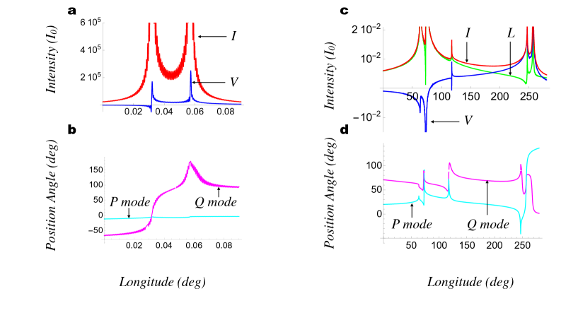
Figure 2: a, Longitudinal distributions of the intensities of the total ($I$) and circularly polarized ($V$) radiation generated by the current sheet in units of $I_{0}$ for the inclination angle $\alpha=5^{\circ}$ at a far-field observation point with the colatitude $\theta_{P}=5^{\circ}$. Distribution of the intensity of the linearly polarized radiation ($L$) is essentially coincident with that of $I$ in this case. The sharp modulations of the pulse profile (its microstructure) are discernible here because this figure is plotted for $k_{\rm u}=10^{2}$ which corresponds to a relatively thick current sheet. The thinner the current sheet, the shorter are the wavelengths of these modulations. At its peak, the right-hand component of this pulse has the intensity $I=1.05\times 10^{12}I_{0}$ and the longitudinal width $6.76\times 10^{-9}$ second when $k_{\rm u}$ is $10^{7}$, i.e., when the thickness of the current sheet is of the order of $10^{-7}c/\omega$. b, Position angles of the two polarization modes versus longitude for the pulse depicted in a. Note that not only does $V$ reverse sign across the left-hand component of this pulse but also the position angle of the $Q$ mode swings through $180^{\circ}$ across the profile of this component. Note also the approximate orthogonality of the two modes over most of the pulse window. c, The Stokes parameters $I$, $L$ and $V$ versus longitude for $\alpha=80^{\circ}$, $\theta_{P}=110^{\circ}$ and $k_{\rm u}=10^{4}$. This is an example of a pulse with several widely separated peaks for which the Stokes parameters are comparable in magnitude over some longitudinal intervals. Though hardly visible, small amplitude sharp modulations pervade also the distribution here. d, Position angles of the two polarization modes versus longitude for the pulse depicted in c exemplifying position-angle distributions that undergo differing variations across different components of the pulse profile. Part d is plotted with $k_{\rm u}=10^{7}$ for clarity.

Two examples of the longitudinal distributions of the Stokes parameters for the radiation generated by the current sheet are shown in Fig. 2. The total intensity $I$ and the intensities of the linearly and circularly polarized components of the radiation, $L$ and $V$, are plotted for given values of the inclination angle $\alpha$ and colatitude $\theta_{P}$ of a far-field observer in units of

$$I_{0}=\left(\frac{\omega B_{0}r_{s0}^{2}}{cR_{P}}\right)^{2},$$ (1)

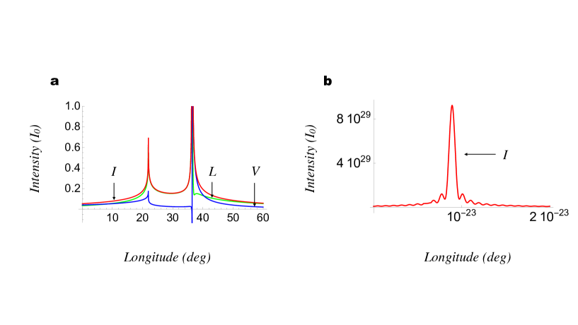
Figure 3: a, Distributions of the Stokes parameters $I$, $L$ and $V$ in units of $I_{0}$ for the inclination angle $\alpha=60^{\circ}$, an observation point in the equatorial plane $\theta_{P}=90^{\circ}$, a distance of $10^{13}$ light-cylinder radii and $k_{\rm u}=10^{7}$. In this example, the colatitude of the observation point lies close to one of the critical colatitudes for the given values of the inclination angle and distance (the colatitudes at which two nearby saddle points of the integral representing the retarded potential coalesce). b, The right-hand component of the pulse depicted in a is here plotted over a sufficiently short longitudinal interval to resolve its peak and width. The values of $\alpha$, $\theta_{P}$, $k_{\rm u}$ and distance in b are the same as in a but the origin of longitude is shifted in b for clarity. The shape of the pulse depicted in b is the same in all cases of this type.

where $B_{0}$ is the magnitude of the star’s dipolar field at its magnetic pole, $r_{s0}$ is the star’s radius and $R_{P}$ is the distance of the observer from the star. In these examples, and in Fig. 3, the origin of the azimuthal coordinate of the observation point is shifted to place the pulse window next to longitude zero. The electric field of the radiation turns out to be the sum of two distinct parts with differing polarization position angles (see §4 of the Supplementary Information). Figure 2 also shows the longitudinal distributions of the position angles of these two parts which we refer to as $P$ and $Q$ modes. Here, those branches of the multi-valued function defining the position angle are adopted that yield continuous position-angle distributions across various components of a given pulse.

The variable $k_{\rm u}^{-1}$, whose value determines the wavelength of the small-amplitude modulations (microstructure) of the distributions shown in Fig. 2, represents a lower limit to the thickness of the current sheet in units of the light-cylinder radius. The thickness assigned to the current sheet by the description in ref. 7 is zero. However, a superluminally moving source is necessarily volume-distributed [17]: it would give rise to a divergent field if it has no thickness. We have circumvented this shortcoming of the description given in ref. 7 by replacing the infinitely long integration range in the Fourier representation of the Dirac delta function describing the current sheet by the truncated wave-number interval $|k|\leq k_{\rm u}$ (see Method).

Figure 3 illustrates an example of a radically different type of pulse: one detectable near those observation points for which two nearby saddle points of the integral over the latitudinal distribution of the current sheet coalesce, thus giving rise to a much tighter focusing of the emitted waves. Though their profiles over the entire pulse window look similar to those of other pulses (as in Fig. 3a), such pulses display extraordinarily large amplitudes and short widths once their peaks are resolved (as in Fig. 3b). We shall see below that the extraordinary values of the amplitudes and widths of such pulses, illustrated by the example in Fig. 3, are what underpin the high brightness temperatures and broad frequency spectra of the radiation generated by the current sheet.

Further examples of pulse profiles and position-angle distributions can be found in the Supplementary Information. It should be added that at any given value of the inclination angle $\alpha$, the pulse observed at $\pi-\theta_{P}$ differs from that observed at $\theta_{P}$ only in that the intensity $V$ of its circularly polarized part is replaced by $-V$ and its longitude $\varphi_{P}$ is replaced by $\varphi_{P}+\pi$. Moreover, the results for $\alpha>\pi/2$ follow from those for $\alpha<\pi/2$ by replacing $\theta_{P}$, $\varphi_{P}$ and $V$ by $\pi-\theta_{P}$, $\varphi_{P}+\pi$ and $-V$, respectively.

2.2 Brightness temperature

By equating the magnitude of the Poynting flux of the radiation to the Rayleigh-Jeans law for the energy that a black body of the same temperature would emit per unit time per unit area into the frequency band $\Delta\nu$ centred on the frequency $\nu$, it can be shown that the brightness temperature of the radiation $T_{\rm b}$ is related to the Stokes parameter $I$ by

$$T_{\rm b}=1.23\times 10^{10}I\,{\hat{T}}_{\rm b}\,\,{}^{\circ}{\rm K}\qquad{\rm with}\qquad{\hat{T}}_{\rm b}=\frac{{\hat{B}}_{0}^{2}d^{4}}{{\hat{P}}^{2}D^{2}{\hat{\nu}}^{2}\Delta{\hat{\nu}}}$$ (2)

in which $I$ is in units of $I_{0}$, ${\hat{B}}_{0}$ is the value of the magnetic field $B_{0}$ in units of $10^{12}$ Gauss, $d$ is the value of the star’s radius $r_{s0}$ in units of $10^{6}$ cm, $D$ is the value of the observer’s distance $R_{P}$ in kpc, ${\hat{\nu}}$ and $\Delta{\hat{\nu}}$ are the values of the radiation frequency and its bandwidth in units of $10^{8}$ Hz and $10^{6}$ Hz, respectively, and ${\hat{P}}=10^{2}/\omega$ is the value of the star’s rotation period in seconds.

Equation (2) yields $T_{\rm b}=1.29\times 10^{22}{\hat{T}}_{\rm b}$ ^∘K for the example depicted in Fig. 2a and $T_{\rm b}=1.17\times 10^{40}{\hat{T}}_{\rm b}$ ^∘K for the example depicted in Fig. 3. (See §4 of the Supplementary Information for other examples including one for which $T_{\rm b}$ is as high as $10^{54}{\hat{T}}_{\rm b}$ ^∘K.)

2.3 Frequency spectrum

Given that the radiation field of the current sheet depends on the observation time $t_{P}$ and the azimuthal coordinate $\varphi_{P}$ of the observation point only in the combination $\varphi_{P}-\omega t_{P}$, the frequency spectrum of this radiation is equally well described by the Fourier decomposition of its longitudinal distribution. In the present case, the content of this spectrum stems from two factors. One factor is the thickness of the current sheet manifested in the sharp small-amplitude modulations of the pulse profile whose wavelengths are proportional to $k_{\rm u}^{-1}$ (see Fig. 1a). The other factor is the full width at half maximum ($\delta\varphi_{P}$) of the component of the pulse profile with the highest peak (see Fig. 3b). While the spectral distribution of the former lies in the radio band when $k_{\rm u}\gtrsim 10^{5}$, that of the latter ranges from radio waves to gamma rays: the width $\delta\varphi_{P}=1.21\times 10^{-26}$ radian of the pulse depicted in Fig. 3b, for example, implies a frequency spectrum that extends as far as $\nu\simeq\omega/(2\pi\delta\varphi_{P})\simeq 1.31\times 10^{27}{\hat{P}}^{-1}$ Hz.

In the lower frequency range, the Stokes parameter $I$ has the power-law dependence $\nu^{-\beta}$ on frequency with a spectral index $\beta$ that assumes the following values in various regimes: $2/3$, $1$, $4/3$, $5/3$, $2$, $7/3$ (see §4 of the Supplementary Information).

2.4 Flux density and its rate of decay with distance

In the present case where the length subtended by the longitudinal extent of the radiation beam embodying a high-frequency pulse can be shorter than $1$ cm at $D=1$ kpc, the flux density ${\cal S}$ of the radiation is related to the Stokes parameter $I$ by

$${\cal S}=2.79\times 10^{-3}\frac{I\,\delta\varphi_{P}}{D^{2}}\,{\cal S}_{0}\,\,\,\,\,\frac{{\rm erg}}{{\rm sec}\times{\rm cm}^{2}}\qquad{\rm with}\qquad{\cal S}_{0}=\left(\frac{{\hat{B}}_{0}d^{2}}{{\hat{P}}}\right)^{2},$$ (3)

in which $I$ is in units of $I_{0}$ and $\delta\varphi_{P}$ in radians. In the case depicted in Fig. 3 where $\alpha=60^{\circ}$, $\theta_{P}=90^{\circ}$ and $k_{\rm u}=10^{7}$, for example, the flux density ${\cal S}$ has the value $32.1\,{\cal S}_{0}$ erg/(sec$\times$cm²) at $D=1$ kpc.

The separation between two nearby saddle points of the integral over the latitudinal distribution of the current sheet decreases as $R_{P}^{-1/2}$ with increasing distance $R_{P}$ of the observation point from the star. The enhanced focusing of the radiation that is caused by this shortening of the separation between the saddle points gives rise to both a narrowing of the width and an augmenting of the peak intensity of the emitted pulse. Because the peak intensity and the width of the pulse are modified with different rates, this effect results in a flux density that diminishes with increasing distance as $R_{P}^{-3/2}$ rather than $R_{P}^{-2}$ (or equivalently as $D^{-3/2}$ instead of $D^{-2}$). The latitudinal width $\delta\theta_{P}$ of such non-spherically decaying pulses is of the order of $(R_{P}\omega/c)^{-1}$ radians in most cases. But there are, in general, several latitudes near which such pulses can be observed; the number and locations of these latitudes are determined by the values of $\alpha$ and $R_{P}$ (see §4 of the Supplementary Information).

The violation of the inverse-square law encountered here is not incompatible with the requirements of the conservation of energy because the radiation process discussed in this paper is intrinsically transitive. The difference in the fluxes of power across any two spheres centred on the star is in this case balanced by the change with time of the energy contained inside the shell bounded by those spheres (see Appendix C of ref. 9 for a demonstration of this feature).

Given their limited latitudinal extent, the non-spherically decaying pulses generated by the current sheet of a neutron star are more likely to be observed when, as a result of the precession of the star’s rotation axis, the radiation beams embodying such pulses sweep past the Earth. Using the decay rate $R_{P}^{-2}$, we would over-estimate the power emitted by the sources of the bursts of radiation we would receive in this way by as large a factor as $10^{14}$ if the neutron stars that generate the bursts lie at cosmological distances. The enormously high energetic requirements normally attributed to the sources of fast radio bursts and gamma-ray bursts [12, 13] could therefore be artefacts of the invariably made assumption that the radiation fields of all sources necessarily decay as predicted by the inverse-square law.

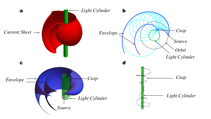
Figure 1: a, Snapshot of a single turn of the current sheet about the light cylinder (the cylinder at which the speed of any entity co-rotating with the neutron star would equal the speed of light $c$). This surface undulates within the latitudinal interval $(\pi/2-\alpha,\pi/2+\alpha)$ each time it turns about the rotation axis, thus wrapping itself around the light cylinder as it extends to the outer edge of the magnetosphere ($\alpha$ which denotes the angle between the magnetic and rotation axes of the star has the value $\pi/3$ in this figure). b, Cross sections of the wave fronts (the circles in light blue) emanating from a volume element of the current sheet with fixed radial and latitudinal coordinates. This figure is plotted for a source element the radius of whose orbit (the dotted circle) is $2.5$ times the radius $c/\omega$ of the light cylinder (the green circle). Cross sections of the two sheets of the envelope of these wave fronts with the plane of the orbit (shown in dark blue) meet at a cusp and wind around the rotation axis, while moving away from it all the way to the far zone. c, Three-dimensional plot of the envelope of wave fronts emanating from a superluminally rotating source element and d, the cusp of this envelope along which the two sheets of the envelope meet tangentially. The cusp touches the light cylinder where it crosses the plane of the orbit and moves away from the axis of rotation as it and the envelope itself spiral into the far zone maintaining a symmetry with respect to this plane.

3 Method

Both the outcomes of the numerical simulations of the magnetosphere of an oblique rotator [3, 4, 5, 6] and their semi-analytic description [7] have appeared in the literature as space-time distributions of the electric and magnetic fields. Once inserted in Maxwell’s equations, the field distributions described in ref. 7 yield the following expressions for the charge and current densities, $\rho^{(cs)}$ and ${\bf j}^{(cs)}$, of the current sheet in terms of the spherical polar coordinates $(r_{s},\theta,\varphi)$ and time $t$:

$$\rho^{(cs)}=-\frac{j_{0}}{c{\hat{r}}_{s}^{2}}\sin\theta\,h\,\delta({\cal C}),$$ (4)

and

$${\bf j}^{(cs)}=\rho^{(cs)}c\,{\hat{\bf e}}_{r_{s}}-\frac{j_{0}}{{\hat{r}}_{s}^{3}}\big{[}\sin\alpha\sin\left({\hat{\varphi}}+{\hat{r}}_{s}-{\hat{r}}_{s0}\right){\hat{\bf e}}_{\theta}+h\,{\hat{\bf e}}_{\varphi}\big{]}\delta({\cal C}),$$ (5)

where

$${\cal C}=\sin\alpha\sin\theta\cos\left({\hat{\varphi}}+{\hat{r}}_{s}-{\hat{r}}_{s0}\right)+\cos\alpha\cos\theta,$$ (6)

$${\hat{\varphi}}=\varphi-\omega t,$$ (7)

$$h=\sin\alpha\cos\theta\cos\left({\hat{\varphi}}+{\hat{r}}_{s}-{\hat{r}}_{s0}\right)-\cos\alpha\sin\theta,$$ (8)

$$j_{0}=0.365\omega B_{0}{\hat{r}}_{s0}^{2}w_{1}w_{3}/\pi,$$ (9)

$$w_{1}=\left|1-2\alpha/\pi\right|,\qquad w_{3}=1+0.2\sin^{2}\alpha,$$ (10)

$\delta$ is the Dirac delta function, ${\hat{r}}_{s}=r\omega/c$, ${\hat{r}}_{s0}=r_{s0}\omega/c$ and $({\hat{\bf e}}_{r_{s}},{\hat{\bf e}}_{\theta},{\hat{\bf e}}_{\varphi})$ are the base vectors of the coordinate system (see §1 of the Supplementary Information).

For the purposes of the present analysis, it is essential that the finiteness of the duration of the source is taken into account (see Appendix B of ref. 9). If $\rho^{(cs)}$ and ${\bf j}^{(cs)}$ are turned on at $t=0$, then the coordinates $t$ and $\varphi$ in equations (4) and (5) both range over $(0,\infty)$ but the values of the combination ${\hat{\varphi}}=\varphi-\omega t$ in which they occur has a limited range of length $2\pi$, e.g.,

$$0\leq{\hat{\varphi}}<2\pi.$$ (11)

As can be seen from the alternative form $\varphi={\hat{\varphi}}+\omega t$ of equation (7), ${\hat{\varphi}}$ is a Lagrangian coordinate that labels the rotating volume elements of the current distribution on each circle $r_{s}=$const, $\theta=$const, by their azimuthal positions at the time $t=0$. This coordinate cannot range over a wider interval because the aggregate of volume elements that constitute a rotating source in its entirety can at most occupy an azimuthal interval of length $2\pi$ at any given time (e.g., at $t=0$).

As pointed out in the text, we have replaced the range of integration in the following Fourier representation of the Dirac delta function that appears in equations (4) and (5),

$$\delta({\cal C})=\frac{1}{2\pi}\int_{-\infty}^{\infty}{\rm d}k\,\exp({\rm i}\,k\,{\cal C}),$$ (12)

by the finite interval $(-k_{\rm u},k_{\rm u})$ to circumvent the divergence that arises from the vanishing of the thickness of the current sheet.

In this paper, the retarded potential

$$\left[\matrix{{\mathbf{A}}({\bf x}_{P},t_{P})\cr\Phi({\bf x}_{P},t_{P})\cr}\right]=\frac{1}{c}\int{\rm d}^{3}{\bf x}\,{\rm d}t\,\left[\matrix{{\mathbf{j}}^{(cs)}({\bf x},t)\cr{\rho^{(cs)}({\bf x},t)c}\cr}\right]\frac{\delta(t-t_{P}+R/c)}{R},\quad t\geq 0,\quad 0\leq{\hat{\varphi}}<2\pi,$$ (13)

that arises from the charge and current densities described by the modified versions of equations (4) and (5) is inserted in

$${\mathbf{E}}=-\nabla_{P}\Phi-\frac{1}{c}\frac{\partial{\mathbf{A}}}{\partial t_{P}},\quad\quad{\mathbf{B}}=\nabla_{P}{\mathbf{\times A}},$$ (14)

to obtain the corresponding expression for the generated radiation field $({\bf E},{\bf B})$, where $({\bf x},t)$ and $({\bf x}_{P},t_{P})$ are the space-time coordinates of the source points and the observation point $P$, respectively, and $R$ is the magnitude of the separation ${\bf R}={\bf x}_{P}-{\bf x}$ (see, e.g., ref. 8).

To satisfy the required boundary conditions at infinity the free-space radiation field of an accelerated superluminal source has to be calculated (in the Lorenz gauge) by means of the retarded solution of the wave equation for the electromagnetic potential. There is a fundamental difference between the classical expression for the retarded potential and the corresponding retarded solution of the wave equation that governs the electromagnetic field. While the boundary contribution to the retarded solution of the wave equation for the potential that appears in Kirchhoff’s surface-integral representation can always be rendered equal to zero by means of a gauge transformation that preserves the Lorenz condition, the corresponding boundary contribution to the retarded solution of the wave equation (or any other equation) for the field cannot be assumed to be zero a priori. Not to exclude emissions whose intensity could decay more slowly than predicted by the inverse-square law, it is essential that the radiation field is derived from the retarded potential (see § 3 of ref. 9 where this point is expounded).

Since the problem discussed in this paper entails the formation of caustics we cannot proceed to the far-field limit $|{\bf x}_{P}|\to\infty$ before evaluating the radiation field, as is customarily done in radiation theory. The far-field approximation of the argument of the delta function in (13) would replace spherical wave fronts by planar wave fronts thereby relinquishing the possibility of their constructive interference. Moreover, given the exceptionally short scales of the longitudinal (or equivalently temporal) variations of the present radiation, it would be intractably more difficult to obtain the time-domain results reported in this paper by means of a frequency-domain analysis (see, e.g., ref. 19). Further technical reasons why a conventional approach to the present problem does not work are discussed in Appendix B of ref. 9.

We calculate the retarded potential (13) in §3 of the Supplementary Information by first performing the integration with respect to $t$ at a fixed $(r_{s},\theta,{\hat{\varphi}})$, i.e., by superposing the contributions of the uniformly rotating volume elements of the current sheet illustrated in Figs. 1b–d. A uniform asymptotic approximation to the value of the integral over $t$, which entails two nearby saddle points, [20] is obtained by the time-domain version of the method of Chester, Friedman and Ursell. [21, 22] The divergences of the resulting expression (which acts as the Green’s function for the problem) on the envelope of the emitted waves and its cusp stem from the relativistic restrictions inherent in Maxwell’s equations and reflect the fact that no superluminal source can be point-like. [17] Once the product of the charge–current density with this Green’s function is integrated over the ${\hat{\varphi}}$ extent of the current sheet with the aid of Hadamard’s regularisation technique, [23, 24] an expression is obtained that is singular only on the hyperboloid swept by the cusp loci of the envelopes of various source elements (see Fig. 1d). This remaining singularity is also removed when the integration with respect to the radial extent of the current sheet is performed: an integration that receives its main contribution from the intersection of the hyperboloid in question with the current sheet. The last integral (that with respect to $\theta$) is singularity-free and once again entails two nearby saddle points that coalesce for certain values of the colatitude $\theta_{P}$ of the observation point.

The five-dimensional integration (with respect to $t$, $r_{s}$, $\theta$, ${\hat{\varphi}}$ and $k$) required for evaluating the radiation field (14) has here been carried out analytically. The only assumption made in the analysis presented in the Supplementary Information is that the radiation frequency appreciably exceeds the rotation frequency $\omega/2\pi$.

A final remark is in order: it is often presumed that the plasma equations used in the numerical simulations of the magnetospheric structure of an oblique rotator should, at the same time, predict any radiation that the resulting structure would be capable of emitting. [3, 4] Irrespective of the formalism on which they are based (whether force-free, MHD or particle-in-cell), the plasma equations used in these simulations are formulated in terms of the electric and magnetic fields (as opposed to potentials). It has already been demonstrated in §3 of ref. 9, however, that the gauge freedom offered by the solution of Maxwell’s equations in terms of potentials plays an indispensable role in the prediction of the characteristics of the present radiation. The absence of high-frequency radiation (and, specifically, the type of radiation described in this paper) is hardwired into the numerical simulations that have been performed to determine the magnetospheric structure of an oblique rotator by the imposition of the standard boundary conditions on the fields in the far zone (see §3 of ref. 9).

4 Supplementary Information

Supplementary Information for this article is included below in the form of a paper, a paper that presents the mathematical derivations of the results reported in the present article.

References

- [1] Beskin, V. S. Radio pulsars: already fifty years! Phys.-Usp., 61, 353–380 (2018).
- [2] Melrose, D. B., Rafat, M. Z. & Masterano, A. Pulsar radio emission mechanisms: a critique. Mon. Not. R. Astron. Soc., 500, 4530–4548 (2021).
- [3] Spitkovsky, A. Time-dependent force-free pulsar magnetospheres: axisymmetric and oblique rotators. Astrophys. J., 648, L51–L54 (2006).
- [4] Kalapotharakos, C., Contopoulos, I. & Kazanas, D. The extended pulsar magnetosphere. Mon. Not. R. Astron. Soc., 420, 2793–2798 (2012).
- [5] Tchekhovskoy, A., Spitkovsky, A. & Li, J. C. Time-dependent 3D magnetohydrodynamic pulsar magnetospheres: oblique rotators. Mon. Not. R. Astron. Soc., 435, L1–L5 (2013).
- [6] Philippov, A. A. & Spitkovsky, A. Ab-initio pulsar magnetosphere: particle acceleration in oblique rotators and high-energy emission modeling. Astrophys. J., 855, article id: 94, 11pp. (2018).
- [7] Tchekhovskoy, A., Philippov, A. & Spitkovsky, A. Three-dimensional analytical description of magnetized winds from oblique pulsars. Mon. Not. R. Astron. Soc., 457, 3384–3395 (2016).
- [8] Jackson, J. D. Classical Electrodynamics, 3rd edn. Wiley (1999).
- [9] Ardavan, H. The electromagnetic radiation whose decay violates the inverse-square law: detailed mathematical treatment of an experimentally realized example. J. Plasma Phys., 85, article id: 905850304, 90 pp. (2019).
- [10] Manchester, R. N. & Taylor, J. H. Pulsars, W. H. Freeman (1978).
- [11] Kaspi, V. M. & Beloborodov, A. M. Magnetars. Ann. Rev., Astron. Astrophys., 55, 261–301 (2017).
- [12] Petroff, E., Hessels, J. W. T. & Lorimer, D. R. Fast radio bursts. Astron. Astrophys. Rev., 27, article id: 4 (2019).
- [13] Piron, F. Gamma-ray bursts at high and very high energies. C. R. Phys., 17, 617–631 (2016).
- [14] Bogovalov, S. V. On the physics of cold MHD winds from oblique rotators. Astron. Astrophys., 349, 1017–1026 (1999).
- [15] Bolotovskii, B. M. & Ginzburg, V. L. The Vavilov-Čerenkov effect and Doppler effect in the motion of sources with superluminal velocity in vacuum. Sov. Phys.-Usp., 15, 184–192 (1972).
- [16] Ginzburg, V. L. Vavilov-Čerenkov effect and anomalous Doppler effect in a medium in which the wave phase velocity exceeds the velocity of light in vacuum. Sov. Phys.-JETP, 35, 92–93 (1972).
- [17] Bolotovskii, B. M. & Bykov, V. P. Radiation by charges moving faster than light. Sov. Phys. Usp., 33, 477–487 (1990).
- [18] Philippov, A., Uzdensky, D. A., Spitkovsky, A. & Cerutti, B. Pulsar radio emission mechanism: radio nanoshots as a low frequency afterglow of relativistic magnetic reconnection. Astrophys. J., 876, L6–L12 (2019).
- [19] Achkasov, V. V. & Zhuravlev, M. Ye. Stationary phase approximation for the Mach surface of superluminally moving source. Reports on Math. Phys., 85, 375–385 (2020).
- [20] Bleistein, N. & Handelsman, R. A. Asymptotic Expansions of Integrals, Dover (1986).
- [21] Burridge, R. Asymptotic evaluation of integrals related to time-dependent fields near caustics. SIAM J. Appl. Math.. 55, 390–409 (1995).
- [22] Chester, C., Friedman, B. & Ursell, F. An extension of the method of steepest descent. Proc. Cambridge Philos. Soc., 53, 599–611 (1957).
- [23] Hadamard, J. Lectures on Cauchy’s Problem in Linear Partial Differential Equations, Dover (2003).
- [24] Hoskins, R. F. Delta Functions: an Introduction to Generalised Functions, 2nd edn. Oxford (2009).