Temporal EigenPAC for dyslexia diagnosis

Abstract

Electroencephalography signals allow to explore the functional activity of the brain cortex in a non-invasive way. However, the analysis of these signals is not straightforward due to the presence of different artifacts and the very low signal-to-noise ratio. Cross-Frequency Coupling (CFC) methods provide a way to extract information from EEG, related to the synchronization among frequency bands. However, CFC methods are usually applied in a local way, computing the interaction between phase and amplitude at the same electrode. In this work we show a method to compute PAC features among electrodes to study the functional connectivity. Moreover, this has been applied jointly with Principal Component Analysis to explore patterns related to Dyslexia in 7-years-old children. The developed methodology reveals the temporal evolution of PAC-based connectivity. Directions of greatest variance computed by PCA are called eigenPACs here, since they resemble the classical eigenfaces representation. The projection of PAC data onto the eigenPACs provide a set of features that has demonstrates their discriminative capability, specifically in the Beta-Gamma bands.

1 Introduction

Developmental Dyslexia (DD) is one learning disability disorders with a higher prevalence, affecting between 5% and 13% of the population  [2]. It has an important social impact causing effects in children like low self-esteem and depression and may be a cause for school failure.

The diagnostic of DD is an important issue for procure the intervention programs that help to adapt the learning process for dyslexic children. In this way, an early diagnosis is essential, which has historically been a complex task due to the use of behavioural tests. These tests depend on the motivation of each children and also have the inconvenient of include writing and reading tasks which postpone the start of diagnosis (i.e. it is not possible to diagnose pre-readers).

This aspect is changing with the use of biomedical signals, which provide objective and quantifiable measures to study the neural basis of the healthy brain and its pathologies. A relevant method to obtain information of brain activity is the electroencephalography (EEG), which allows to acquire brain signals in a non-invasive way. This technique can be used to quantify the functional activity of the brain while developing a specific task. In particular, EEG signals have been used to explore the neurological origin of DD in  [3, 4, 5], towards the advance in the knowledge of dyslexia and its objective diagnosis.

One way to build functional models that help to understand the brain processes developed while the subject is developing a specific task, is through connectivity. In other words, it consists in measuring how the different brain areas cooperates in any manner while processing information. On the other hand, neural oscillations are produced mainly in five frequency bands: Delta (0.5-4) Hz, Theta (4-8) Hz, Alpha (8-12) Hz, Beta (12-30) Hz and Gamma ($>$ 30 Hz). The exploration of the relationship among these bands has demonstrated to provide useful information to characterize the brain activity. This way, Cross Frequency Coupling (CFC) is a technique to explore interactions and (also called couplings) between frequency bands and has undergone and special attention in recent years.

In the present work, EEG signals are used to explore the functional connectivity. Specifically, the Phase Amplitude Coupling (PAC), a type of CFC, is calculated to analyze and identify temporal patterns in dyslexic and non-dyslexic subjects. Then, Principal Component Analysis (PCA) is used for identify and extract patterns in order to perform a classification using SVM for a differential diagnosis.

The paper is organized as follows. Section 2 presents details of the database and describes the auditory stimulus and the methods used. Then, Section 3 presents and discusses the classification results, and finally, Section 5 draws the main conclusions and the future work.

2 Materials and Methods

2.1 Database and stimulus

The EEG data used in this work was provided by the Leeduca Study Group at the University of Málaga  [6]. EEG signals were recorded using the Brainvision acticHamp Plus with 32 active electrodes (actiCAP, Brain Products GmbH, Germany) at a sampling rate of 500 Hz during 15 minutes sessions, while presenting an auditory stimulus to the subject. A session consisted of a sequence of white noise stimuli modulated in amplitudes at rates 2, 8, and 20 Hz presented sequentially for 5 minutes each.

The present experiment was carried out with the understanding and written consent of each child’s legal guardian and in the presence thereof. Forty-eight participants took part in the present study, including 32 skilled readers (17 males) and 16 dyslexic readers (7 males) matched in age (t(1) = -1.4, p $>$ 0.05, age range: 88-100 months). The mean age of the control group was 94, 1 $\pm$ 3.3 months, and 95, 6 $\pm$ 2.9 months for the dyslexic group. All participants were right-handed Spanish native speakers with no hearing impairments and normal or corrected–to–normal vision. Dyslexic children in this study have all received a formal diagnosis of dyslexia in the school. None of the skilled readers reported reading or spelling difficulties or have received a previous formal diagnosis of dyslexia. The locations of 32 electrodes used in the experiments is in the 10–20 standardized system.

2.2 Signal Prepocessing

The EEG signals recorded were processed to remove artifacts related to eye blinking and impedance variation due to movements. It was used blind source separation with Independent Component Analysis (ICA) to remove artifacts corresponding to eye blinking signals in the EEG signals. Then, EEG signal of each channel was normalized independently to zero mean and unit variance and referenced to the signal of electrode Cz. Baseline correction was also applied. Finally, the EEG signals were segmented into 15.02 s long windows in order to analyze PAC temporal patterns correctly  [7]. This is the minimum appropriate window length for which a sufficiently high number of slow oscillation cycles are analyzed, shorter windows lead to overestimates of coupling and lower significance. This adequate window length is one of the main requisites for robust PAC estimation and appropriate statistical validation of the result by surrogate tests without using long data windows that assumes stationarity of the signals within the window.

2.3 Phase-Amplitude Coupling (PAC)

Cross-frequency coupling(CFC) has been proposed to coordinate neural dynamics across spatial and temporal scales [8], it serve as a mechanism to transfer information from large scale brain networks and has a potential relevance for understanding healthy and pathological brain function. In particular, Phase-Amplitude Coupling has received significant attention  [7, 10] and may play an important functional role in local computation and long-range communication in large-scale brain networks [9].

PAC describes the coupling between the phase of a slower oscillation and the amplitude of a faster oscillation. Concretely, in this work we explore the modulation of the amplitude of the Gamma (30–100) Hz frequency band by the phase of the Delta (0.5-4) Hz, Theta (4-8) Hz, Alpha(8-12) Hz and Beta(12-25) Hz bands. There are different PAC descriptors for measuring PAC  [1]. In this work, we use the Modulation Index (MI) [12, 11], although there is no convention yet of how to calculate phase-amplitude coupling and much heterogeneity of phase-amplitude calculation methods used in the literature  [13].

For calculating MI as in [11], first all phases are binned into eighteen 20 degrees intervals and the average amplitude of the amplitude-providing frequency in each phase bin of the phase-providing frequency is computed and normalized by the following formula:

$$p(j)=\frac{\bar{a}}{\sum^{N}_{j=1}\bar{a}_{k}}$$ (1)

where $\bar{a}$ is the average amplitude of one bin, $k$ is the running index for the bins, and $N=18$ is the total amount of bins; $p$ is a vector of $N$ values.

Then, Shannon entropy H(p) is computed by means of

$$H(p)=-\sum^{N}_{j=1}P(j)log{P(j)}$$ (2)

where $p$ is the vector of normalized averaged amplitudes per phase bin. This represents the inherent amount of information of a variable. If the Shannon entropy is maximal, all the phase bins present the same amplitude (uniform distribution). Thus, the existence of phase-amplitude coupling is characterized by a deviation of the amplitude distribution from the uniform distribution in a phase-amplitude plot. To measure this, the Kullback–Leibler (KL) distance of a discrete distribution $P$ from a distribution $Q$ is used and it is defined as

$$KL(P,Q)=\sum^{N}_{j=1}P(j)log\frac{P(j)}{Q(j)}$$ (3)

and the KL distance is relate to the Shannon entropy by the following formula

$$KL(U,P)=logN-H(p)$$ (4)

where U is the uniform distribution and P is the amplitude distribution defined earlier by p(j) **? Finally, the raw MI is calculated by the following formula:

$$MI=\frac{KL(U,X)}{logN}$$ (5)

In this work, PAC is measured by MI in each data segment, enabling the exploration of the temporal evolution of the response to specific auditory stimuli. This is achieved with the use of Tensorpac  [14], an open-source Python toolbox dedicated to PAC analysis of neurophysiological data. Tensorpac provides a set of efficient methods and functions to implements the most common PAC estimation methods, such as the Modulation Index used in the present work.

2.4 Dimensionality Reduction and Classification

Principal Component Analysis (PCA) is a widely used method to perform dimensionality reduction. It is a well known multivariate analysis technique used in many studies  [15, 16] to significantly reduce the original high-dimensional feature space to a lower-dimensional subspace spanned by a number (n) of Principal Components (PC), while preserving the variation of the dataset in the original space as much as possible.

A well known application of PCA the so-called eigenimage decomposition, which results from the application of PCA to images. This is used in different works such as  [17, 18] and adapted from the eigenface approach of Turk and Pentland  [19]. In this work this approach is used allowing to detect underlying patterns that differentiate individuals within a population, even if the differences are subtle.

Here, PCA is applied in the time axis to compute the maximum variance directions of the PAC along the EEG segments. Thus, we obtain the PCs or eigenvectors of the covariance matrix of the a dataset composed by N vectors, corresponding to the MI values of each 31 electrodes for the ten segments of every subject. These eigenvectors describe a set of features that characterize the variation between the PAC measured in each temporal segment. As usual, they are sorted in decreasing explained variance order. We can display these eigenvectors in topoplots, representing the principal components at each electrode position. In order to keep the traditional notation, we called these PC as eigenPACs. Then, we selected the eigenPACs that have the largest eigenvalues which therefore account for the most variance within the set of PAC matrix, composing a M-dimensional subspace.

For the sake of clarity, let the measured PAC vector set be $\Gamma_{1},\Gamma_{2},...,\Gamma_{N}$ of length equal to the number of electrodes. The average PAC of the dataset is defined as $\Gamma=\frac{1}{N}\sum^{N}_{n=1}\Gamma_{n}$. Each measured PAC differs from the average by the vector $\Phi_{i}=\Gamma_{i}-\Gamma$ with $i=1,2,...,N$. On this set, a PCA transformation is applied obtaining $M$ orthogonal vectors $u_{i}$ which best describes the distribution of the data. This vectors satisfy that

$$\lambda_{1}=\frac{1}{N}\sum^{N}_{n=1}(u^{T}_{i}\Phi_{n})^{2}$$ (6)

is maximum, subject to

$$u^{T}_{i}u_{j}=\delta_{ij}$$ (7)

where $\delta_{ij}$ is the Kronecker delta, and $u_{i}$ and $\lambda_{i}$ are the eigenvectors and eigenvalues, respectively, of the covariance matrix:

$$C=\frac{1}{N}\sum^{N}_{n=1}\Phi_{n}\Phi^{T}_{i}=AA^{T}$$ (8)

where the matrix $A={\Phi_{1},...,\Phi_{N}}$. These eigenvectors are what we refer as eigenPAC. Usually, the first few eigenPACs explain almost the whole variance, so only a number $M^{\prime}<M$ is necessary to appropriately describe the dataset  [18]. Thus, the computacional complexity of the diagonalization process to obtain the eigenPAC basis is significantly reduced.

In essence, the eigenPACs define a new space in which each component explains the maximum variance in the data represented by its eigenvalue and its correlation is minimized. The projection of the PAC vectors onto the eigenPAC space, will determine the coordinates of each PAC vector in this subspace. It is expected that this projection produce a pattern more suitable for class separation than the projection onto the average PAC space, due to the eigenPAC decorrelation  [17].

For the classification we use this projections of the data on the new basis to train a Support Vector Machine (SVM). Hence, the PAC vectors measured for the ten segments EEG signals are projected on the eigenPAC basis obtaining $N$ vectors each of them with its corresponding class label defined as control and dyslexic. Then, using the training data the SVM separates this set of binary labelled data with a hyperplane that is maximally distant from the two classes [18].

3 Experimental Results

In this section, we show the experimental results obtained in with the PAC analysis, eigenPAC representation and classification. As mentioned before, the EEG data was segmented into ten temporal windows of 15.02 s for the analysis of the temporal evolution of the response to the stimulus. This analysis was performed with the measure of PAC over each segment.

3.0.1 PAC Results

To analyze PAC connectivity we used the tensorpac tool  [14]. Thus, we defined the frequency bands in which the PAC is measured (phase band and amplitude band) and we expected an identifiable temporal behaviour. This set of frequency band pairs are: Delta-Gamma, Theta-Gamma, Alpha-Gamma and Beta-Gamma. We measured the PAC for each subject and each temporal segment obtaining results for all the frequency bands. This results are represented with a set of ten topoplots showing the temporal evolution of the average PAC of dyslexic subjects and control subjects in each frequency pair. Figure. 1 shows the differences between the average MI value for the dyslexic group and the control group. In this Figure we represented each combination of frequency bands for which the PAC has been measured. These topoplots denote differences between the response of dyslexic and control subjects.

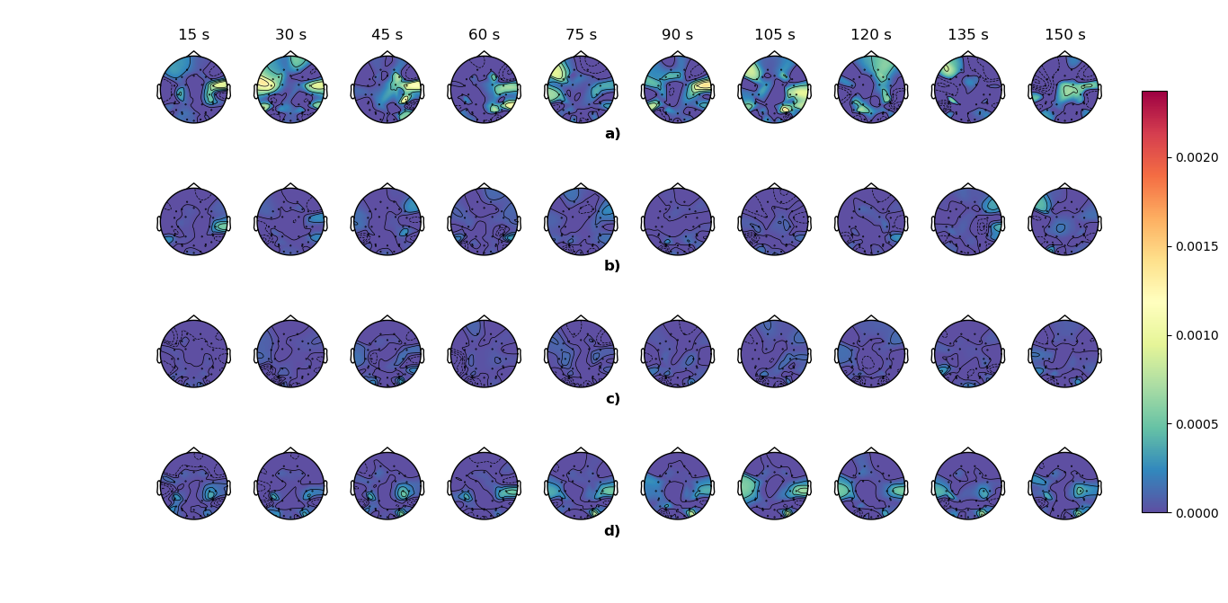
Figure 1: Difference average MI topoplot for 2 Hz. a) Delta-Gamma b)Theta-Gamma c)Alpha-Gamma d)Beta-Gamma

3.0.2 EigenPAC Results

PCA has been applied in two different ways. In the first case, PAC features from all the subjects have been used to obtain the PCs, as in the case of eigenfaces problem. This aims to obtain a representation of the overall database in terms of the maximum variance directions. To carry out this experiment, a matrix is created containing the MI value computed from temporal segments of all subjects. Specifically, this matrix contains N*(number of segments) rows corresponding to the number of subjects multiplied by the number of segments and M columns corresponding to MI of each of the 31 electrodes. Then, PCA is applied and we obtain a set of PCs of which the first five represent the most part of the variance. In Fig. 2 we can see the representation of the eigenPAC for the first 5 PC indicating the area where there is a major temporal variation in the measured MI for the Beta-Gamma PAC. This eigenPAC are different for each stimulus and the first topoplot describes the maximal data variation.

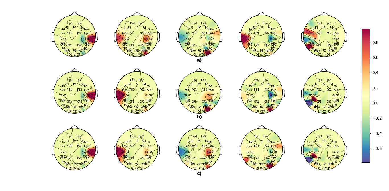
Figure 2: First 5 eigenPAC for Beta-Gamma. a)2 Hz b) 8 Hz c) 20 Hz

A second experiment is performed by applying PCA to dyslexic and control groups separately. This results similar as the previous case, but only with subjects of one group. Thus, we achieve a better representation of the temporal variation for each group, obtaining a set of PCs describing the maximal variation for the dyslexic subjects and another set of PCs for the control subjects. These eigenPAC, represented in Fig. 3, show the variation specifically related to the temporal response to the auditory stimulus. As shown, we found global similarities for each group. Furthermore, this helps to identify the characteristic patterns of each class that are used by classifications algorithms reaching a better performance.

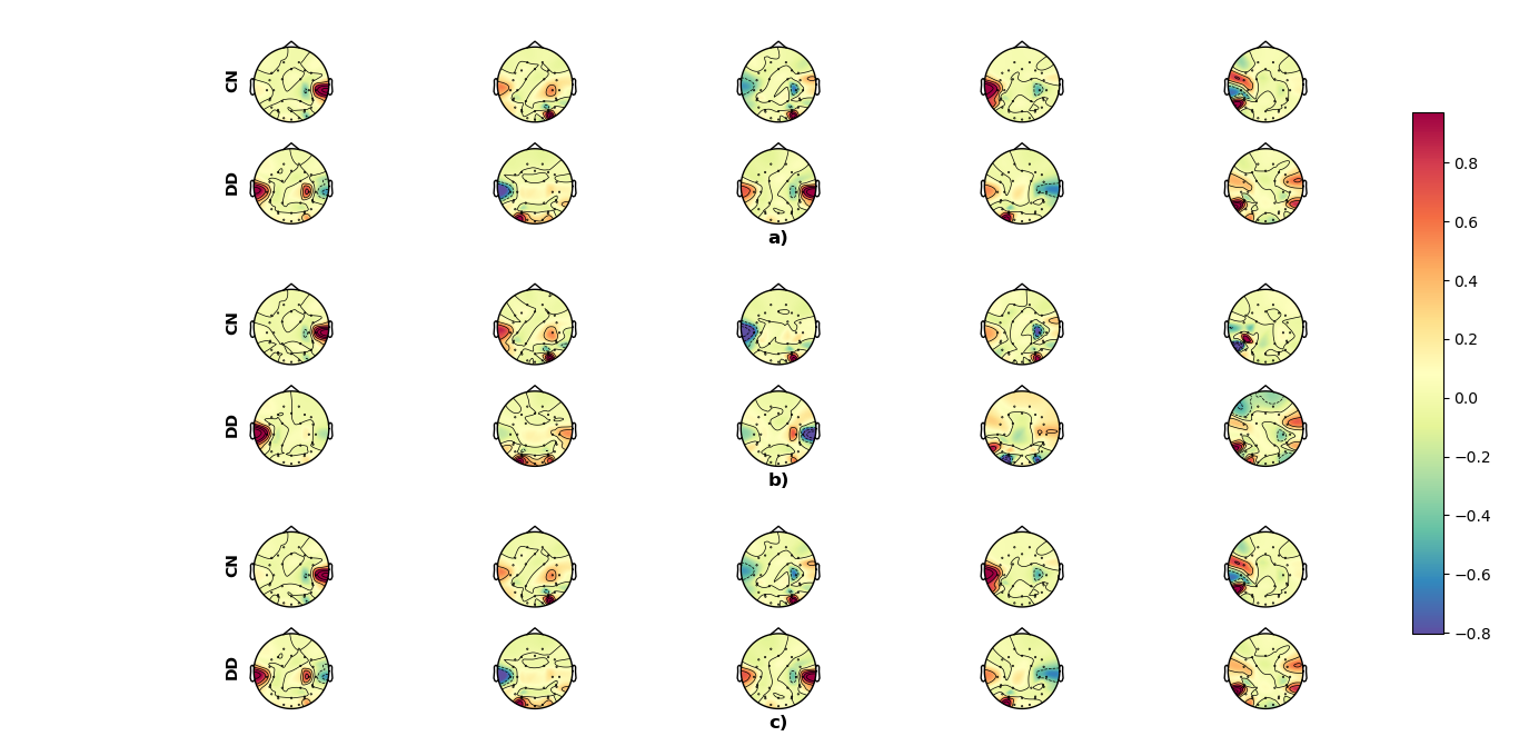
Figure 3: First 5 eigenPAC. a)2 Hz b) 8 Hz c) 20 Hz

In Fig. 3, for each case there are represented in the upper row the topoplots containing the information related to control eigenPAC and in the row below the dyslexic eigenPAC.

3.0.3 Classification

Once the application cases of PCA are defined, we used the resulting eigenPAC to train a SVM classifier. Therefore, there are two ways of perform a classification depending on how we compute the PCs that form the eigenPAC. These are used to project the data into the lower-dimensional space to obtain the feature space of the SVM classifier.

In the first case, the PCs are obtained from the application of PCA over all the subjects, dyslexic and control. Then, this PCs correspond to the eigenPAC that we use to project the data for the SVM. In this part, a k-fold stratified cross validation scheme is employed to separate the data into train sets and test set, specifically, 5-fold cross-validation is used.

In the second case, the application of PCA separately over the two classes provide a set of PCs for each class. Then each subject data is projected onto the control and DD components, and these projections are concatenated to compose the feature vector. The process of cross validation is the same as in the above case just with a different set of PCs.

The metrics used in the classification are the accuracy, sensitivity, specificity and Area Under ROC curve (AUC). The evaluation metrics are described in Table 1. The results show the performance of the two classification scenarios for the best case, which corresponds to the Beta-Gamma PAC as represented in Fig. 4. We can see that there is a improvement related with the application of PCA separately for the two classes.

Table 1: Classification comparative using the Beta-Gamma PAC

Metrics	PCA with all the subjects			PCA with each class separately
	2 Hz	8 Hz	20 Hz	2 Hz	8 Hz	20 Hz
Accuracy	0.572	0.611	0.561	0.654	0.653	0.594
Sensitivity	0.501	0.551	0.515	0.651	0.635	0.551
Specificity	0.743	0.757	0.675	0.661	0.696	0.7
AUC	0.65	0.705	0.622	0.699	0.721	0.65

Therefore, the second case generate higher metrics achieving a better classification performance with a greater AUC and accuracy for 2 Hz, 8 Hz and 20 Hz. We present the results for this case in Fig. 4 where the max AUC is represented for each band combination and each stimulus. Showing that in the Beta-Gamma there are temporal pattern that are distinctive of each class.

Figure 4: Max AUC for each band combination and stimulus

In the case of Beta-Gamma we perform a PC number sweep obtaining the explained variance and the max AUC for the classification with each number of components in Fig. 5

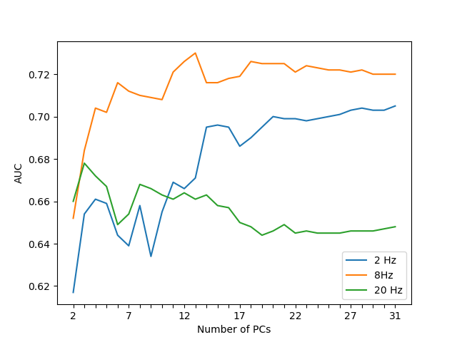
Figure 5: Max AUC for each number of PCs

4 Conclusions and Future Work

In this work we present a classification method for EEG signals based on the study of functional connectivity PAC and the use of eigenPAC resulting of applying PCA to train a SVM classifier. The concept of eigenPAC helps to extract the underlying pattern that differentiates the temporal response between control and dyslexic subjects. Also, it can be represented in topographic plots to visualize the areas with a greater variation principally corresponding to the temporal evolution.

The classification results suggest differential patterns in the Beta-Gamma bands that allows to discriminate between control and dyslexic subjects, obtaining the highest AUC for the 8 Hz stimulus. This points the bands in which the response to the stimulus has differences across the temporal segments and encourage continuing the approach shown in this work. As future work, it is interesting to study the effect of using other windows length and to improve the necessary PAC analysis with the use of decomposition methods such as MEMD to accurately extracts the oscillatory components of the EEG signals.

Acknowledments

This work was partly supported by the MINECO/FEDER under PGC2018-098813-B-C32 project. We gratefully acknowledge the support of NVIDIA Corporation with the donation of one of the GPUs used for this research. Work by F.J.M.M. was supported by the MICINN “Juan de la Cierva - Formación” Fellowship. We also thank the Leeduca research group and Junta de Andalucía for the data supplied and the support.

References

- [1] Tabassum, T.M., Munia, K., Aviyente, S. (2019). Time-Frequency Based Phase-Amplitude Coupling Measure For Neuronal Oscillations. Scientific Reports. 9. 1-15. 10.1038/s41598-019-48870-2.
- [2] Peterson RL, Pennington BF. Developmental dyslexia. Lancet. 2012 May 26;379(9830):1997-2007. \doi 10.1016/S0140-6736(12)60198-6. Epub 2012 Apr 17. PMID: 22513218; PMCID: PMC3465717.
- [3] Power AJ, Colling LJ, Mead N, Barnes L, Goswami U. Neural encoding of the speech envelope by children with developmental dyslexia. Brain Lang. 2016 Sep;160:1-10\doi10.1016/j.bandl.2016.06.006. Epub 2016 Jul 17. PMID: 27433986; PMCID: PMC5108463.
- [4] Ortiz A., Martínez-Murcia F.J., Formoso M.A., Luque J.L., Sánchez A. (2020) Dyslexia Detection from EEG Signals Using SSA Component Correlation and Convolutional Neural Networks. In: de la Cal E.A., Villar Flecha J.R., Quintián H., Corchado E. (eds) Hybrid Artificial Intelligent Systems. HAIS 2020. Lecture Notes in Computer Science, vol 12344. Springer, Cham. \doihttps://doi.org/10.1007/978-3-030-61705-9-54
- [5] Ortiz A., López P., Luque J., Martínez-Murcia F., Aquino-Britez D., Ortega J., An Anomaly Detection Approach for Dyslexia Diagnosis Using EEG Signals, In: Ferrández Vicente J., Álvarez-Sánchez J., de la Paz López F., Toledo Moreo J., Adeli H. (eds) Understanding the Brain Function and Emotions. IWINAC 2019., vol. 11486, 2019.
- [6] Ortiz A, Martinez-Murcia FJ, Luque JL, Giménez A, Morales-Ortega R, Ortega J. Dyslexia Diagnosis by EEG Temporal and Spectral Descriptors: An Anomaly Detection Approach. Int J Neural Syst. 2020 Jul;30(7):2050029.\doi10.1142/S012906572050029X. Epub 2020 Jun 4. PMID: 32496139.
- [7] Dvorak D, Fenton AA. Toward a proper estimation of phase-amplitude coupling in neural oscillations. J Neurosci Methods. 2014 Mar 30;225:42-56. \doi10.1016/j.jneumeth.2014.01.002. Epub 2014 Jan 19. PMID: 24447842; PMCID: PMC3955271.
- [8] Aru J, Aru J, Priesemann V, Wibral M, Lana L, Pipa G, Singer W, Vicente R. Untangling cross-frequency coupling in neuroscience. Curr Opin Neurobiol. 2015 Apr;31:51-61. \doi 10.1016/j.conb.2014.08.002. Epub 2014 Sep 15. PMID: 25212583.
- [9] Ryan T. Canolty, Robert T. Knight,The functional role of cross-frequency coupling, Trends in Cognitive Sciences,Volume 14,Issue 11, 2010, Pages 506-515,ISSN 1364-6613, \doihttps://doi.org/10.1016/j.tics.2010.09.001.
- [10] van der Meij R, Kahana M, Maris E. Phase-amplitude coupling in human electrocorticography is spatially distributed and phase diverse. J Neurosci. 2012 Jan 4;32(1):111-23. \doi10.1523/JNEUROSCI.4816-11.2012 PMID: 22219274; PMCID: PMC6621324.
- [11] Tort, A. B. L., Komorowski, R., Eichenbaum, H., and Kopell, N. (2010). Measuring phase-amplitude coupling between neuronal oscillations of different frequencies. J. Neurophysiol. 104, 1195–1210.\doi10.1152/jn.00106.2010
- [12] Tort, A. B. L., Kramer, M. A., Thorn, C., Gibson, D. J., Kubota, Y., Graybiel, A. M., et al. (2008). Dynamic cross-frequency couplings of local field potential oscillations in rat striatum and hippocampus during performance of a T-maze task. Proc. Natl. Acad. Sci. U.S.A. 105, 20517–20522. \doi10.1073/pnas.0810524105
- [13] Hülsemann MJ, Naumann E, Rasch B. Quantification of Phase-Amplitude Coupling in Neuronal Oscillations: Comparison of Phase-Locking Value, Mean Vector Length, Modulation Index, and Generalized-Linear-Modeling-Cross-Frequency-Coupling. Front Neurosci. 2019 Jun 7;13:573. \doi 10.3389/fnins.2019.00573. PMID: 31275096; PMCID: PMC6592221.
- [14] Combrisson E, Nest T, Brovelli A, Ince RAA, Soto JLP, Guillot A, et al. (2020) Tensorpac: An open-source Python toolbox for tensor-based phase-amplitude coupling measurement in electrophysiological brain signals. PLoS Comput Biol 16(10): e1008302. https://doi.org/10.1371/journal.pcbi.1008302
- [15] Abdulhamit Subasi, M. Ismail Gursoy, EEG signal classification using PCA, ICA, LDA and support vector machines,Expert Systems with Applications,Volume 37, Issue 12,2010,Pages 8659-8666,ISSN 0957-4174, https://doi.org/10.1016/j.eswa.2010.06.065.
- [16] P.J. Markiewicz, J.C. Matthews, J. Declerck, K. Herholz, Robustness of multivariate image analysis assessed by resampling techniques and applied to FDG-PET scans of patients with Alzheimer’s disease,NeuroImage,Volume 46, Issue 2,2009,Pages 472-485,ISSN 1053-8119,https://doi.org/10.1016/j.neuroimage.2009.01.020.
- [17] I.A. Illán, J.M. Górriz, J. Ramírez, D. Salas-Gonzalez, M.M. López, F. Segovia, R. Chaves, M. Gómez-Rio, C.G. Puntonet,18F-FDG PET imaging analysis for computer aided Alzheimer’s diagnosis,Information Sciences,Volume 181, Issue 4,2011,Pages 903-916,ISSN 0020-0255,https://doi.org/10.1016/j.ins.2010.10.027.
- [18] Alvarez, Górriz. “Alzheimer’s Diagnosis Using Eigenbrains and Support Vector Machines.” Bio-Inspired Systems: Computational and Ambient Intelligence. Berlin, Heidelberg: Springer Berlin Heidelberg. 973–980. Web.
- [19] Turk, Pentland. “Eigenfaces for Recognition.” Journal of Cognitive Neuroscience, vol. 3, no. 1, MIT Press, Jan. 1991, pp. 71–86, doi:10.1162/jocn.1991.3.1.71.