Nonextensive Boltzmann Transport Equation: the Relaxation Time Approximation and Beyond

Abstract

We derive approximate iterative analytical solutions of the nonextensive Boltzmann transport equation in the relaxation time approximation. The approximate solutions almost overlap with the exact solution for a considerably wide range of the parameter values found in describing particle spectra originated in high-energy collisions. We also discuss the Landau kinetic approximation of the nonextensive Boltzmann transport equation and the emergence of the nonextensive Fokker-Planck equation, and use it to estimate the drag and diffusion coefficients of highly energetic light quarks passing through a gluonic plasma.

I Introduction

Studying the transport properties of a medium is an important field of research which helps characterizing a system. One of the most widely used transport equations is the Boltzmann Transport Equation (BTE) degroot derived long ago for a dilute gas of classical particles. Since then, it has been used in many fields including that of high energy collisions. For example, to understand the transport of particles inside the quark-gluon plasma medium produced in high energy collisions, either the BTE, or some approximated version of it has been used Yao:2020xzw ; Qiao:2020yry ; Kurian:2019nna ; Singh:2018wps ; Tripathy:2017nmo ; tsallisraaepja ; Mazumder:2011nj . In this approach, the evolution of a distribution function is studied, and is utilized to understand the observables in the multi-particle production experiments colliding protons or heavy-ions. Investigating the properties of such a medium calls for a statistical approach which is conventionally based on the Boltzmann-Gibbs statistics and the exponential single particle distribution which is obtained as a stationary state solution of the conventional BTE. It is, however, observed that the BTE may be inadequate to describe freeze-out in high energy collision experiments Magas:2005mb . Also, conditions leading to the Boltzmann-Gibbs statistics may not be satisfied because systems produced rather display long-range correlation and fluctuation. For strongly interacting plasmas like the QGP, the plasma parameter $\Gamma$ given by the ratio of the average potential to kinetic energy is larger than 1. In these situations, interaction length is much larger than the Debye screening length and a strongly interacting plasma like QGP does not follow the conventional kinetic equation leading to equilibration of system. It can be shown that for such a system, power-law stationary states like the one characterized by the Tsallis statistics arise rafelskiwaltonprl .

Imprints of nonextensivity are also found in the hadronic transverse momentum distributions which are power-like, and hence, are far from being exponential. Such a power-like distribution which is routinely used in the field of high-energy collisions is proportional to the following factor jpg20 ; Cleymans:2013rfq ,

$$\left(1+\frac{q-1}{T}E\right)^{-\frac{q}{q-1}},$$ (1)

which originates from the Tsallis statistics Tsal88 . In Eq. (1), $E=\sqrt{|\vec{P}|^{2}+m^{2}}$ is the single particle energy for a particle with three-momentum $\vec{P}$ and mass $m$. $q$ is the entropic parameter, and $T$ is the Tsallis temperature. The $q$ parameter is related to the relative variance in temperature (or number of particles) which is reminiscent of the fluctuating ambiance Wilk00 ; Wilk09 . Also, analyzing scaling properties of the Yang-Mills theory, $q$ is deduced from field theory parameters like $N_{c}$ (no. of colours) and $N_{f}$ (no. of flavours) deppmanprdq . When, $q\rightarrow$1, the ‘Tsallis factor’ (represented as the $q$-exponential $\exp_{q}$ raised to the power $q$) approaches being Boltzmann-like (exponential), i.e.

$$\lim_{q\rightarrow 1}\left(1+\frac{q-1}{T}E\right)^{-\frac{q}{q-1}}=\lim_{q\rightarrow 1}\left\{\exp_{q}\left(-\frac{E}{T}\right)\right\}^{q}=\exp\left(-\frac{E}{T}\right).$$ (2)

It is found that Eq. (1), which describes the high-energy collision data, is the stationary solution of a modified Boltzmann transport equation lavagnopla ; wilkosada ; Biro:2012ix inspired by the Tsallis statistics for a non-equilibrium distribution $f$,

$$P^{\mu}\partial_{\mu}f^{q}=\mathcal{C}_{q}[f].$$ (3)

One of the modifications in the Tsallis-inspired Boltzmann transport equation in Eq. (3), henceforth to be called the nonextensive BTE (NEBTE), is that the distribution function at the left hand side is raised to the power $q$. This power is important for conservation laws to hold lavagnopla . The collision term $\mathcal{C}_{q}$ is also modified to accommodate a generalization of the ‘molecular chaos’ (stosszahlansatz) hypothesis which may not be valid in the system produced in high-energy collisions. It is to be noted that when $q\rightarrow 1$, the NEBTE converges to the conventional BTE.

Analytical solutions of the conventional Boltzmann transport equation exist under certain approximations. One such example is the relaxation time approximation. Solution of the BTE under this approximation considering simplifying scenarios is well-studied and has been subject matters in recent studies involving the Tsallis-like distributions tsallisraaepja ; maciej ; Wilk:2021jpl . In Ref. Wilk:2021jpl , authors also consider the time variation of the Tsallis $q$ parameter to go beyond the relaxation time approximation.

Under the same simplifying assumptions of a homogeneous plasma with no external force, the NEBTE under the relaxation time approximation (RTA) is non-linear because of the power index $q$ in the l.h.s of Eq. (3). And hence, unlike the BTE, finding an exact, and closed analytical solution is difficult. In the present paper, we compute approximate iterative analytical solutions of the nonextensive BTE in the relaxation time approximation. We observe that the approximate solutions almost overlap with the exact solution for a considerably wide range of the parameter values. In addition to this, we also discuss the Landau kinetic approximation of the NEBTE and the emergence of the nonextensive Fokker-Planck equation (see also Ref. hqtsfp ; deppmannnefpe ). Later, this equation has been used to estimate the drag and diffusion coefficients of energetic light quarks passing through a gluonic plasma.

II nonextensive Boltzmann transport equation

If we expand the l.h.s of Eq. (3) assuming that there is no net external force, we obtain,

$$\frac{\partial f^{q}(\vec{P},\vec{r},t)}{\partial t}+\vec{v}.\vec{\nabla}f^{q}(\vec{P},\vec{r},t)=E^{-1}\mathcal{C}_{q}[f(\vec{P},\vec{r},t)],$$ (4)

where for a particle with three-momentum magnitude $|\vec{P}|\equiv\sqrt{P_{t}^{2}+P_{z}^{2}}$ (where $P_{t}$ and $P_{z}$ are transverse and longitudinal momenta respectively), and energy $E$, velocity $v=|\vec{P}|/E$, and $\vec{r}$ denotes the position coordinates. Assuming an expansion along the collision axis which is taken to be the z-direction,

$$\frac{\partial f^{q}(\vec{P},z,t)}{\partial t}+v_{z}\frac{\partial f^{q}(\vec{P},z,t)}{\partial z}=E^{-1}\mathcal{C}_{q}[f(\vec{P},z,t)].$$ (5)

Under the Bjorken’s assumption of boost-invariance at the central rapidity region, Eq. (5) can be written as Baym ,

$$\left.\frac{\partial f^{q}(\vec{P}_{t},P_{z},t)}{\partial t}\right|_{P_{z}t}=E^{-1}\mathcal{C}_{q}[f(\vec{P}_{t},P_{z},t)].$$ (6)

For the binary collisions of particles with four-momenta $P\equiv(E,\vec{P})$ (having the momentum distribution $f$), and $Q\equiv(\mathcal{E},\vec{Q})$ (having the momentum distribution $g$), which become $P^{\prime}\equiv(E^{\prime},\vec{P^{\prime}})$, and $Q^{\prime}\equiv(\mathcal{E^{\prime}},\vec{Q^{\prime}})$ after interaction, the collision term of the nonextensive Boltzmann transport equation can be written as wilkosada ; Biro:2012ix ,

$$\mathcal{C}_{q} = \frac{1}{2}\int\frac{d^{3}\vec{Q}}{(2\pi)^{3}\mathcal{E}}\frac{d^{3}\vec{Q^{\prime}}}{(2\pi)^{3}\mathcal{E^{\prime}}}\frac{d^{3}\vec{P^{\prime}}}{(2\pi)^{3}E^{\prime}}|\overline{M}|^{2}(2\pi)^{4}\delta^{4}(P+Q-P^{{}^{\prime}}-Q^{{}^{\prime}})\left[h_{q}\{f(\vec{P^{\prime}}),g(\vec{Q^{\prime}})\}-h_{q}\{f(\vec{P}),g(\vec{Q})\}\right].$$

$M$ is the amplitude of the quark-quark or quark-gluon collisional processes in a quark-gluon plasma medium. The function $h_{q}$ is a generalization of the molecular chaos hypothesis, and combines the two distributions $f$, and $g$ in the following way,

$$h_{q}\{f,g\}=\exp_{q}\left[\log_{q}(f)+\log_{q}(g)\right],$$ (8)

where

$$\log_{q}f=\frac{1-f^{1-q}}{q-1}.$$ (9)

Here $\log_{q}$ is the $q$-logarithm function and becomes the conventional logarithm in the limit $q\rightarrow 1$, which also implies,

$$\lim_{q\rightarrow 1}h_{q}\{f,g\} = \lim_{q\rightarrow 1}\exp_{q}\left[\log_{q}(f)+\log_{q}(g)\right]$$ (10)

$$= \exp\left[\log(f)+\log(g)\right]$$

$$= f\times g,$$

i.e., the distribution functions are independent, which is a consequence of the molecular chaos hypothesis. In this limit, one gets back the collision term of the conventional BTE svetitsky ,

$$\mathcal{C} = \frac{1}{2}\int\frac{d^{3}\vec{Q}}{(2\pi)^{3}\mathcal{E}}\frac{d^{3}\vec{Q^{\prime}}}{(2\pi)^{3}\mathcal{E^{\prime}}}\frac{d^{3}\vec{P^{\prime}}}{(2\pi)^{3}E^{\prime}}|\overline{M}|^{2}(2\pi)^{4}\delta^{4}(P+Q-P^{{}^{\prime}}-Q^{{}^{\prime}})\left[f(\vec{P^{\prime}})g(\vec{Q^{\prime}})-f(\vec{P})g(\vec{Q})\right].$$

The form of the collision term in Eq. (II) is motivated by the fact that in strongly interacting systems, one needs a transport equation whose stationary solution is given by a power-law distribution. The conventional Boltzmann transport equation that considers stosszahlansatz in the collision term yields only an exponential distribution and a generalization leads to a Tsallis power-law stationary solution. The generalized stosszahlansatz indicates an interplay between the probe particle and medium particle distributions. In this article, this interplay has been characterized using the $q$ functions. A deformed Fokker-Planck equation (that will be considered in a later section), just like the generalized Boltzmann transport equation, also leads to a power-law stationary solution and can adequately describe traversal of highly energetic particles inside strongly interacting QCD medium.

III nonextensive Boltzmann transport equation in the relaxation time approximation

If at time $t=0$, all the external forces are switched off and the gradient is cancelled, the nonextensive Boltzmann transport equation for the distribution $f$ in the relaxation time approximation is given by silvanebterta (except for the power $q$, as discussed in lavagnopla ),

$$\frac{\partial f^{q}}{\partial t} = -\frac{\left(f-f_{\text{eq}}\right)}{\tau}$$

$$\frac{\partial f}{\partial t} = -\frac{\left(f^{2-q}-f_{\text{eq}}f^{1-q}\right)}{q\tau},$$ (12)

where $\tau$ is the relaxation time. Integrating the above equation,

$$\int\frac{df}{\left(f^{2-q}-f_{\text{eq}}f^{1-q}\right)} = \mathcal{K}-\theta$$

$$\frac{1}{q-1}\int\frac{dw}{\left(1-f_{\text{eq}}w^{-\frac{1}{q-1}}\right)} = \mathcal{K}-\theta,\quad$$

$$\text{where}\quad w\equiv f^{q-1},\quad\theta=\frac{t}{q\tau},$$ (13)

and $\mathcal{K}$ is the integration constant which may be obtained from the boundary condition, $f(t=0)=f_{\text{in}}$, where $f_{\text{in}}$ is the initial distribution. We expand the integrand in a negative binomial series and integrate.

$$\frac{1}{q-1}\int dw\left(1+f_{\text{eq}}w^{-\frac{1}{q-1}}+f_{\text{eq}}^{2}w^{-\frac{2}{q-1}}+...\right) = \mathcal{K}-\theta\quad\left(\left|f_{\text{eq}}w^{-\frac{1}{q-1}}\right|\equiv\left|\frac{f_{\text{eq}}}{f}\right|<1\right)$$

$$\Rightarrow\frac{f^{q-1}}{q-1}{{\sum}}_{s=0}^{\infty}\frac{(1)_{s}(1-q)_{s}}{s!(2-q)_{s}}\left(\frac{f_{\text{eq}}}{f}\right)^{s} = \mathcal{K}-\theta$$

$$\Rightarrow\frac{f^{q-1}}{q-1}\,_{2}F_{1}\left(1,1-q;2-q;\frac{f_{\text{eq}}}{f}\right) = \mathcal{K}-\theta,$$

where $`(.)_{s}$’ in the second line is the rising Pochhamer symbol given by abst ,

$$(a)_{s}=\begin{cases}1&s=0\\ a(a+1).....(a+s-1)&\forall s>0,\end{cases}$$ (15)

and $\,{}_{2}F_{1}$ is the hypergeometric function Bateman . The integration constant is given by,

$$\mathcal{K}=\frac{f_{\text{in}}^{q-1}}{q-1}\,_{2}F_{1}\left(1,1-q;2-q;\frac{f_{\text{eq}}}{f_{\text{in}}}\right).$$ (16)

Hence, the solution of the nonextensive Boltzmann transport equation in the relaxation time approximation may be obtained once we solve Eq. (LABEL:nebtesol) for $f$. Although the solution of Eq. (LABEL:nebtesol) can be found using numerical methods, in this paper we calculate approximate analytical expressions for the solutions using the series expansion of the hypergeometric function given in the second line of Eq. (LABEL:nebtesol).

It is straightforward to find the zeroth order solution of Eq. (LABEL:nebtesol) (i.e. for $s=0$) from the following equation,

$$\Psi_{0} = f^{q-1}-(q-1)\left(\mathcal{K}-\theta\right)=0$$

$$\Rightarrow f_{0} = \left[(q-1)\left(\mathcal{K}-\theta\right)\right]^{\frac{1}{q-1}}.$$ (17)

The first order equation, whose solution we denote by $f_{1}(t)$, is given by,

$$\Psi_{1} = f^{q-1}+\left(\frac{1-q}{2-q}\right)f_{\text{eq}}f^{q-2}-(q-1)\left(\mathcal{K}-\theta\right)=0.$$ (18)

And the exact solution, which we denote by $f_{\text{e}}(t)$, is obtained from the following equation,

$$\Psi_{\text{e}}=\frac{f^{q-1}}{q-1}\,_{2}F_{1}\left(1,1-q;2-q;\frac{f_{\text{eq}}}{f}\right)-\mathcal{K}-\theta=0$$ (19)

Though it is straightforward to obtain the zeroth order solution using the inverse function, for the first order and beyond, it becomes difficult.

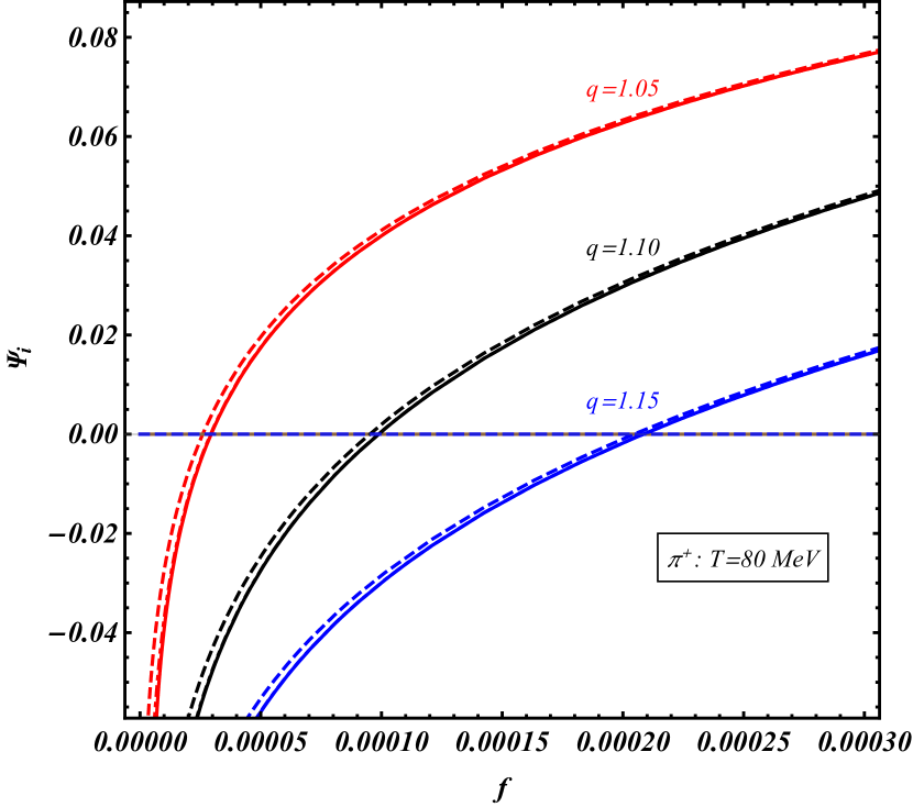
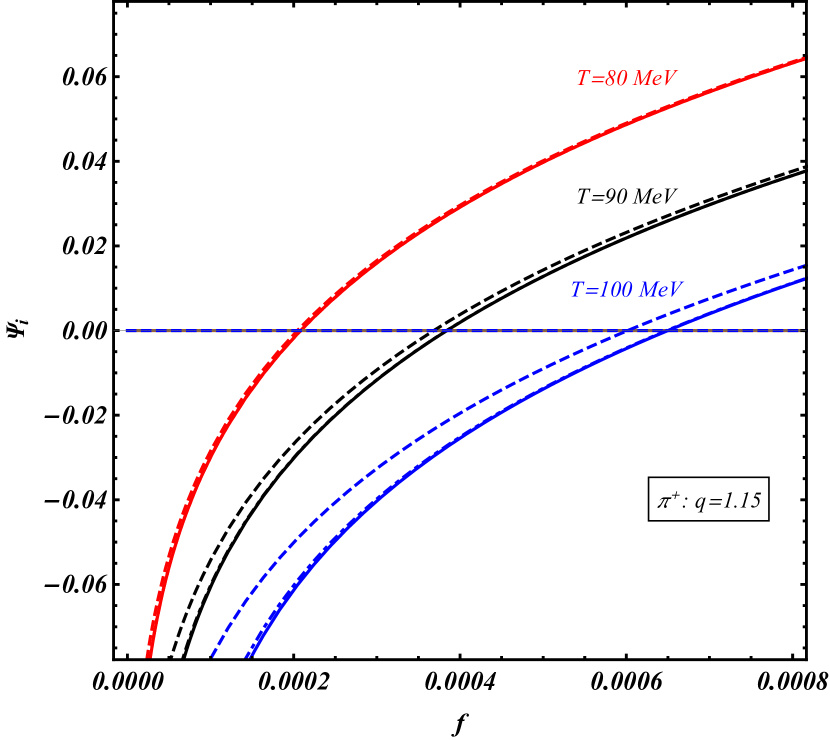
Figure 1: Graphical solutions of Eqs. (17)-(19) for different $q$ and $T$ values, mass $m=139.57$ MeV (pion mass), $p_{\text{T}}$=1 GeV, $q\theta=0.11$.

In what follows, we propose an approximate analytical first order solution for the nonextensive Boltzmann transport equation in the relaxation time approximation. This proposal is based on Fig. 1 which finds the graphical solutions of Eqs. (17), (18), and (19), which are located at the points where $\Psi_{i}^{s}$ ($i=0,1$, e) change sign. We observe that at the transverse momentum values near 1 GeV and above, the solution of the zeroth order equation (dashed line) is very close to that of the exact equation (solid line) which entirely overlaps with the solution of the first order equation (dot-dashed line, not always visible because of overlapping). Hence, we propose to write the solution of the first order equation as a tiny increment over that of the zeroth order in the following way,

$$f_{1}=f_{0}+\epsilon_{1},\quad|\epsilon_{1}|<<f_{0}.$$ (20)

Afterwards, we put Eq. (20) in Eq. (18), expand in terms of $\epsilon_{1}$ up to the first order (since $\epsilon_{1}$ is a small quantity), solve for $\epsilon_{1}$ and get $f_{1}$ in terms of $f_{0}$ whose analytical form is already known from Eq. (17). This gives us the following expression for the solution of the first order equation,

$$f_{1}\approx f_{0}+\frac{f_{0}}{f_{0}+f_{\text{eq}}}\left[\frac{f_{\text{eq}}}{2-q}+\frac{f_{0}}{1-q}+f_{0}^{2-q}\left(\mathcal{K}-\theta\right)\right].$$

(21)

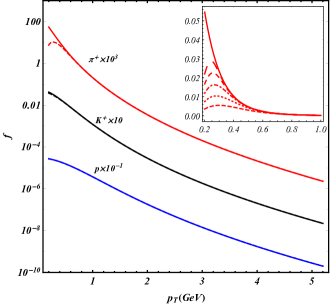
Figure 2: Comparison between the exact and the first order approximated solutions. $q=1.15,~{}T=80$ MeV, and $\theta=0.096$.

Next, we find out how good the approximate solution Eq. (21) is, and if there are any limitations of the approximation. To do this, we compare the exact numerical solution of Eq. (12) and the approximate solution given by Eq. (21) in Fig. 2 for $q=1.15,~{}T=80$ MeV, and $\theta=0.096$. We use the mass values of the pions, kaons and protons. We find that for the pions having very low transverse momentum ($\lesssim$ 0.6 GeV), the approximated solution Eq. (21) underestimates the exact solution. For mass values lower than the pion mass, this disagreement at very low transverse momentum remains. However, for the most part of the pion spectrum, the first order approximation works really well. For heavier particles like the kaons and the protons, the first order approximated solution is as good as the exact solution for the whole spectrum. In the inset of Fig. 2 we plot the zeroth order (bottommost) to the fourth order (second from the top) solutions (for a particle with pion mass) along with the exact solution (red, solid). We observe that higher order solutions lead to a greater degree of agreement between the approximate analytical solution and the exact solution at very low momentum. Following Eq. (20), the first order and the higher order solutions can be represented as,

$$~{}~{}~{}~{}~{}~{}~{}~{}~{}~{}~{}~{}~{}~{}~{}~{}~{}~{}~{}~{}~{}~{}~{}~{}~{}f_{i}=f_{i-1}+\epsilon_{i},\quad i=1,~{}2,~{}3,...,$$ (22)

where $\epsilon_{i}^{\text{s}}$ are calculated from the following equation,

$$\epsilon_{i}=\frac{f_{i-1}}{{\sum}_{r=0}^{i}f_{\text{eq}}^{r}f_{i-1}^{i-r}}\left(f_{i-1}^{i+1-q}(\mathcal{K}-\theta)+{{\sum}}_{r=0}^{i}\frac{f_{\text{eq}}^{r}f_{i-1}^{i-r}}{r+1-q}\right).$$

IV Nonextensive Fokker-Planck equation and its relation to the nonextensive Boltzmann transport equation

The Stratonovich form of the nonextensive Fokker-Planck equation for a function $f^{\prime}({\mathbb{x}})$, where ${\mathbb{x}}\in\mathbb{R}^{N}$ is a dimensionless state variable, is given by borland ,

$$\frac{\partial f^{\prime}}{\partial t}=-\frac{\partial}{\partial x}\left(K(x)f^{\prime}\right)+\frac{\partial}{\partial x}\left(D(x)\frac{\partial f^{\prime 2-q}}{\partial x}\right)$$ (24)

in one dimension. $K$, and $D$ are drift and diffusion. Putting $\partial f^{\prime}/\partial t=0$, the normalized stationary solution of Eq. (24) is,

$$f^{\prime}=\Gamma\left[1-\beta(1-q)V_{\text{eff}}(x)\right]^{\frac{1}{1-q}},$$ (25)

where $\beta$, and $\Gamma$ are appropriate constants with

$$V_{\text{eff}}(x)=-\int\frac{K(x)}{D(x)}dx.$$ (26)

For the drift and diffusion terms,

$$K(x)=-c_{K}x^{\gamma};\quad D(x)=c_{D}x^{r},\quad\text{and}\quad s=\gamma-r+1,$$ (27)

The ansatz for a time ($t$)-dependent solution is written to be borland

$$f^{\prime}(t)=\Gamma(t)\left[1-\beta(t)(1-q)x^{s}\right]^{\frac{1}{1-q}}.$$ (28)

By putting the ansatz in Eq. (24), the time dependence of $\beta$, and $\Gamma$ can be calculated.

It is, however, also possible to get the nonextensive Fokker-Planck equation from Eq. (6) when the Landau approximation is imposed landau . The Landau approximation is motivated by the fact that the most of the parton-parton collisions are soft. That means that the collision rate is the highest near the three-momentum transfer $\vec{k}=\vec{P}-\vec{P^{\prime}}=\vec{Q^{\prime}}-\vec{Q}\approx 0$. To establish this equation, we consider the passage of high-energy light quarks, whose distributions evolve like Eq. (6), through a gluonic medium which is thermalized in the Tsallis sense at a temperature $T_{g}$. The gluonic distribution $g(Q)$ is given by

$$g=\left(1+(q-1)\frac{|\vec{Q}|}{T_{g}}\right)^{-\frac{1}{q-1}}.$$ (29)

We also assume that the shape of the evolving hard quark distribution is dictated by the Tsallis-like function so that,

$$f=\left(1+(q-1)\frac{E}{T}\right)^{-\frac{1}{q-1}}.$$ (30)

Using Eqs. (29), and (30) in the definition Eq. (10), the collision term reads,

$$\mathcal{C}_{q} = \frac{1}{2}\int\frac{d^{3}\vec{Q}}{(2\pi)^{3}\mathcal{E}}\frac{d^{3}\vec{Q^{\prime}}}{(2\pi)^{3}\mathcal{E}^{\prime}}\frac{d^{3}\vec{P^{\prime}}}{(2\pi)^{3}E^{\prime}}|\overline{M}|^{2}(2\pi)^{4}\delta^{4}(P+Q-P^{{}^{\prime}}-Q^{{}^{\prime}})\times$$

$$\left[\left(1+(q-1)\frac{E^{\prime}}{T}+(q-1)\frac{|\vec{Q^{\prime}}|}{T_{g}}\right)^{-\frac{1}{q-1}}-\left(1+(q-1)\frac{E}{T}+(q-1)\frac{|\vec{Q}|}{T_{g}}\right)^{-\frac{1}{q-1}}\right]$$

$$= \frac{1}{2}\int\frac{d^{3}\vec{Q}}{(2\pi)^{3}\mathcal{E}}\frac{d^{3}\vec{Q^{\prime}}}{(2\pi)^{3}\mathcal{E^{\prime}}}\frac{d^{3}\vec{P^{\prime}}}{(2\pi)^{3}E^{\prime}}|\overline{M}|^{2}(2\pi)^{4}\delta^{4}(P+Q-P^{{}^{\prime}}-Q^{{}^{\prime}})\left[f_{|\vec{P}-\vec{k}|}\mathcal{S}_{|\vec{P}-\vec{k}|,|\vec{Q}+\vec{k}|}-f_{|\vec{P}|}\mathcal{S}_{|\vec{P}|,|\vec{Q}|}\right],$$

where $f_{\vec{P}}\equiv f$, $E^{\prime}=\sqrt{|\vec{P^{\prime}}|^{2}+m^{2}}=\sqrt{|\vec{P}-\vec{k}|^{2}+m^{2}}$, and $f_{|\vec{P}-\vec{k}|}$ is the corresponding distribution. $\vec{Q^{\prime}}=\vec{Q}+k$, and

$$\mathcal{S}_{|\vec{P}|,|\vec{Q}|}=\left(1+\frac{(q-1)\frac{|\vec{Q}|}{T_{g}}}{1+(q-1)\frac{E}{T}}\right)^{-\frac{1}{q-1}}.$$ (32)

Expanding Eq. (IV) around $\vec{k}\approx 0$, we obtain the Ito form borland of the nonextensive Fokker-Planck equation from Eq. (6),

$$\frac{\partial f}{\partial t}=-\frac{\partial}{\partial P_{i}}\left(A_{i,q}f\right)+\frac{\partial}{\partial P_{i}\partial P_{j}}\left(B_{ij,q}f^{2-q}\right)~{}~{}~{}~{}~{}~{}~{}~{}(i=1,2,3),$$ (33)

where $A_{i,q}$, and $B_{ij,q}$, the nonextensive Fokker-Planck drag and diffusion coefficients are given by,

$$A_{i,q} = \frac{1}{2Eq}\int\frac{d^{3}\vec{Q}}{(2\pi)^{3}\mathcal{E}}\frac{d^{3}\vec{Q^{\prime}}}{(2\pi)^{3}\mathcal{E^{\prime}}}\frac{d^{3}\vec{P^{\prime}}}{(2\pi)^{3}E^{\prime}}|\overline{M}|^{2}(2\pi)^{4}\delta^{4}(P+Q-P^{{}^{\prime}}-Q^{{}^{\prime}})f^{1-q}S_{\vec{P},\vec{Q}}(P-P^{\prime})_{i}\equiv\left<\left<(P-P^{\prime})_{i}\right>\right>_{q}$$

$$B_{ij,q} = \frac{f^{q-1}}{2}\left<\left<(P-P^{\prime})_{i}(P-P^{\prime})_{j}\right>\right>_{q}.$$ (34)

For a similar approach following the Boltzmann-Gibbs statistics see jalqprd .

V Results

V.1 NEBTE in the RTA

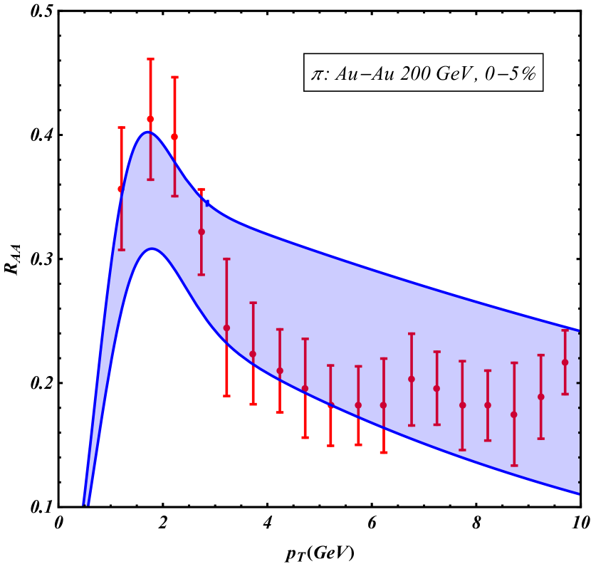
Figure 3: $R_{\text{AA}}$ of neutral pions. $q=1.005\pm 0.003$, $T=0.066\pm 0.024$ GeV, $t/\tau=1.047\pm 0.096$, $\chi^{2}/\text{NDF}=18.64/15$.

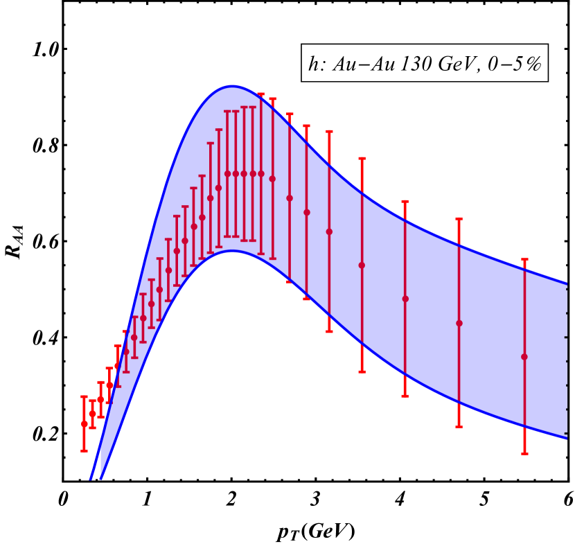
Figure 4: $R_{\text{AA}}$ of all charged hadrons. $q=1.024\pm 0.011$, $T=0.187\pm 0.050$ GeV, $t/\tau=1.183\pm 0.0104$, $\chi^{2}/\text{NDF}=19.09/27$.

We can use the solution $f_{1}$ given by Eq. (21) to describe (for a similar approach considering the conventional BTE see

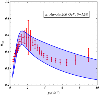
Figure 5: $R_{\text{AA}}$ of charged pions. $q=1.049\pm 0.020$, $T=0.156\pm 0.036$ GeV, $t/\tau=0.394\pm 0.065$, $\chi^{2}/\text{NDF}=23.38/25$.

Ref. tsallisraaepja ) an experimental observable like the nuclear suppression factor $R_{\mathrm{AA}}$ which is experimentally defined by,

$$R_{\mathrm{AA}}=\frac{\left(d^{2}N/dp_{\mathrm{T}}dy\right)^{\mathrm{A+A}}}{N_{\mathrm{coll}}\times\left(d^{2}N/dp_{\mathrm{T}}dy\right)^{\mathrm{p+p}}}.$$ (35)

$N_{\mathrm{coll}}$ is the number of nucleon-nucleon binary collisions (p+p) while a nucleus ‘A’ collides with another nucleus. $d^{2}N/dp_{\mathrm{T}}dy$ denotes the differential yield within the transverse momentum and rapidity range $p_{\rm{T}}$ to $p_{\mathrm{T}}+dp_{\mathrm{T}}$ and $y$ to $y+dy$. If the yield from the nucleus-nucleus collisions would have been a linear superposition of nucleon-nucleon collisions, $R_{\mathrm{AA}}$ would have been 1. Deviation of $R_{\mathrm{AA}}$ from 1 signifies medium modification. Theoretically, $R_{\mathrm{AA}}$ of the hadrons (‘h’) can be computed from the following equation,

$$R_{\mathrm{AA}}=\frac{\sum_{\text{a}}\int f_{1}^{\text{a}}(p_{\text{a}},z)\left.\right|_{p_{\text{a}}=p_{\text{T}}/z}D_{\text{a}/\text{h}}(z)dz}{\sum_{\text{a}}\int f_{\text{in}}^{\text{a}}(p_{\text{a}},z)\left.\right|_{p_{\text{a}}=p_{\text{T}}/z}D_{\text{a}/\text{h}}(z)dz},$$ (36)

where $p_{\text{a}}$ is the momentum of the partons (denoted by ‘a’) which fragment to the hadrons carrying the $z$ fraction of the partonic momentum. $D_{\text{a}/\text{h}}$ is the fragmentation function fragnpb ; fragprd . Description of $R_{\mathrm{AA}}$ data with the help of Eq. (36) is given in Figs. 4 (for the neutral pions pi0phenix200 ), 4 (for all the charged hadrons starhad130 ), and 5 (for the charged pions chpistar200 ). The shaded regions in the figures correspond to the error bars in the parameter values obtained in the fitting.

V.2 Nonextensive Fokker-Planck transport coefficients of the light quarks

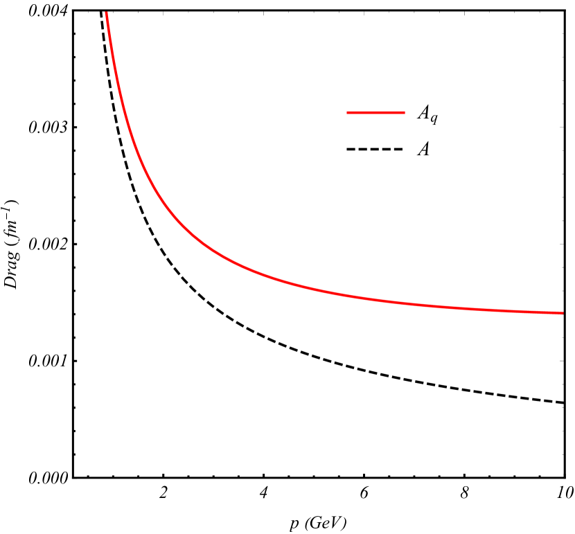
Figure 6: Momentum variation of the nonextensive and extensive drag coefficients of the light quarks.

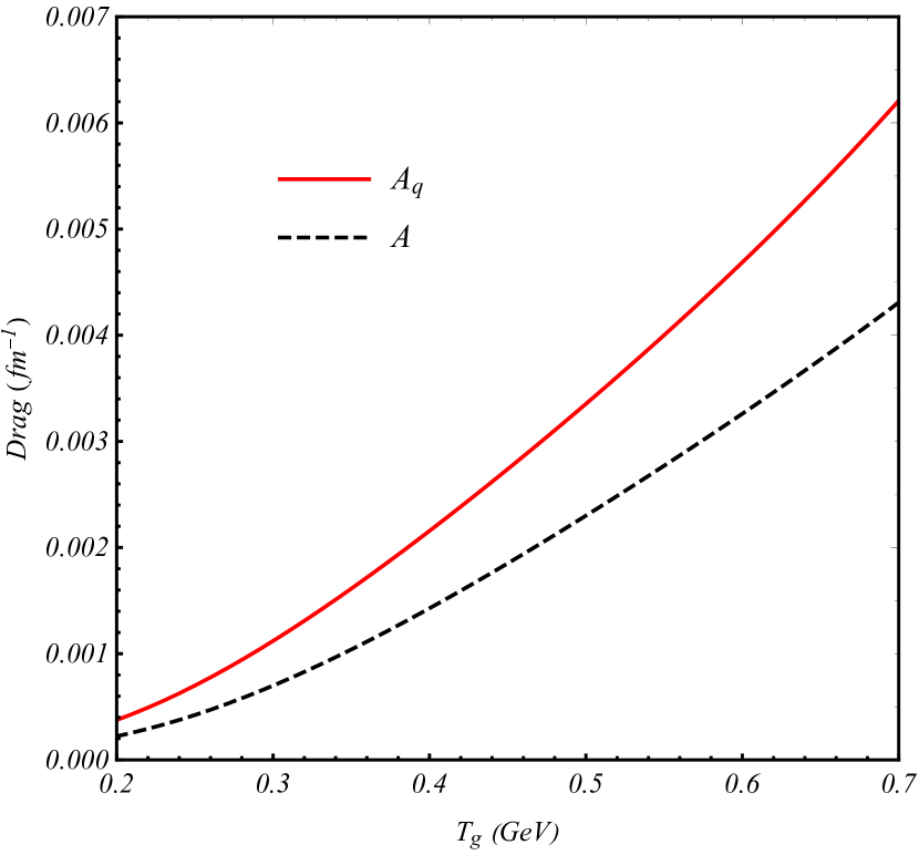
Figure 7: Temperature variation of the nonextensive and extensive drag coefficients of the light quarks.

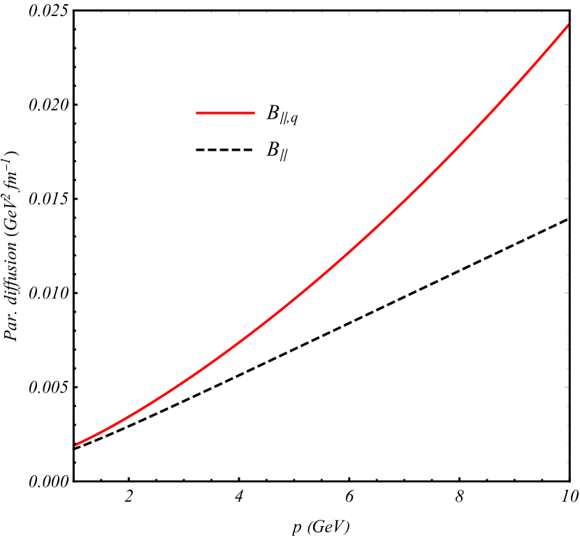
Figure 8: Momentum variation of the nonextensive and extensive parallel diffusion coefficients of the light quarks.

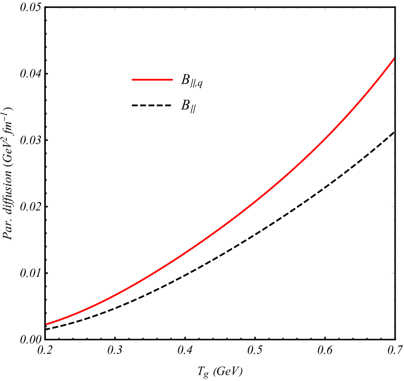
Figure 9: Temperature variation of the nonextensive and extensive parallel diffusion coefficients of the light quarks.

In this section we estimate the nonextensive Fokker-Planck drag and diffusion coefficients of energetic light quarks passing through a gluonic plasma with the help of Eq. (34). We express the nonextensive drag and diffusion coefficients in the following way,

$$A_{i,q} = \frac{P_{i}}{|\vec{P}|^{2}}A_{q}(|\vec{P}|^{2}),$$

$$B_{ij,q} = \left(\delta_{ij}-\frac{{P_{i}}{P_{j}}}{{|\vec{P}|^{2}}}\right)B_{\bot,q}({|\vec{P}|^{2}})+\frac{{P_{i}}{P_{j}}}{{|\vec{P}|^{2}}}B_{||,q}(|\vec{P}|^{2}),$$ (37)

and evaluate $A_{q}$, $B_{\bot,q}$, and $B_{||,q}$ which, from Eq. (34), can be evaluated to be,

$$A_{q} = \left<\left<1-\frac{\vec{P}.\vec{P^{\prime}}}{|\vec{P}|^{2}}\right>\right>_{q},$$

$$B_{\bot,q} = \frac{f^{q-1}}{4}\left<\left<|\vec{P}|^{\prime 2}-\frac{(\vec{P}.\vec{P}^{\prime})^{2}}{|\vec{P}|^{2}}\right>\right>_{q},$$

$$B_{||,q} = \frac{f^{q-1}}{2}\left<\left<\frac{(|\vec{P}|^{2}-\vec{P}.\vec{P}^{\prime})^{2}}{|\vec{P}|^{2}}\right>\right>_{q}.$$ (38)

In the limit $q\rightarrow 1$ they converge with the results given by the Boltzmann-Gibbs statistics. The momentum and temperature variation of the quantities are given in Figs. 9-11. We have taken $q=1.01$, and temperature to be 350 MeV (for Figs. 9, 9, 11), and momentum of the energetic light quark to be 5 GeV (for Figs. 9, 9, 11).

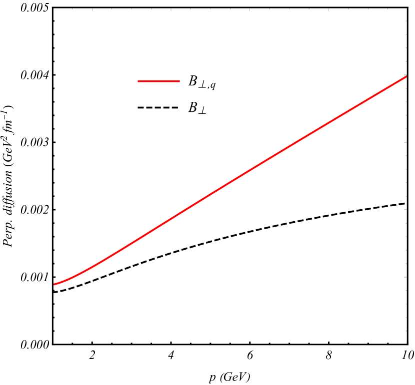
Figure 10: Momentum variation of the nonextensive and extensive perpendicular diffusion coefficients of the light quarks.

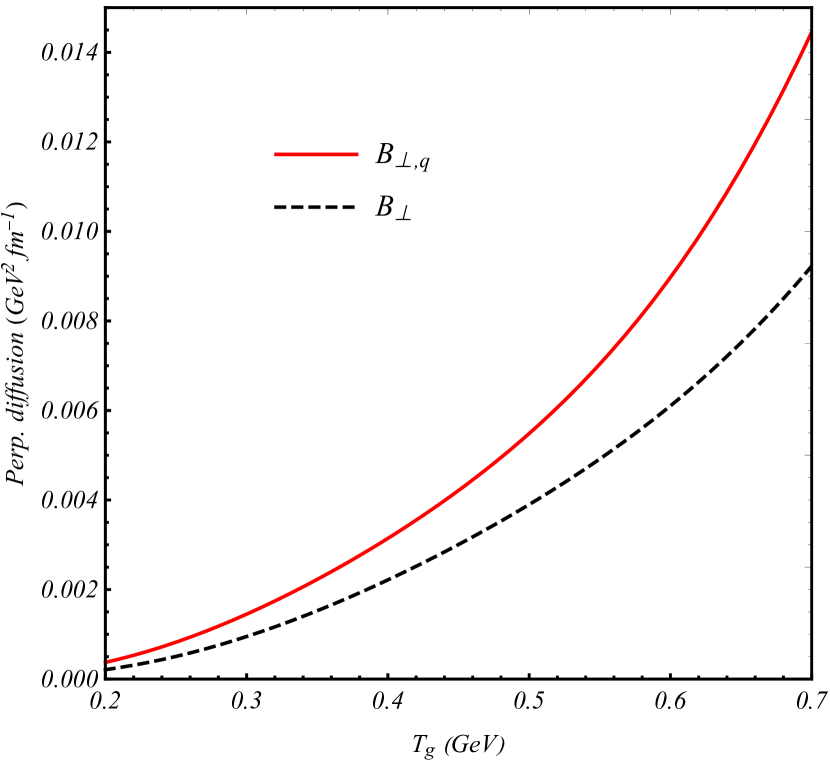
Figure 11: Temperature variation of the nonextensive and extensive perpendicular diffusion coefficients of the light quarks.

VI Summary, conclusions, and outlook

In summary, we have studied the nonextensive Boltzmann transport equation in different approximations. First we have proposed approximate analytical iterative closed form solutions for the NEBTE in the relaxation time approximation and have indicated how the results can be used to describe the nuclear suppression factor (for a similar work using the conventional Boltzmann transport equation, see Ref. tsallisraaepja ).

We have observed that for a considerably wide range of the parameter values relevant for the high-energy physics phenomenology the first order solution is very close to the exact solution. However, this approximated solution works better for higher mass particles. For the lower mass region ($\sim$140 MeV), slight deviation is observed at very low transverse momentum region ($\lesssim$0.6 GeV). The extent of agreement can be increased considering higher order solutions.

From Figs. 4-5, apart from the Tsallis parameter and temperature, we can get an estimate of the ratio of the time scales relevant for evolution processes. We notice that the ratio of the freeze-out time to the relaxation time ($t/\tau$) has a value of the order of 1. An estimate of this quantity has recently been done in Ref. maciej using the conventional Boltzmann transport equation which finds this value to be of the order of 1.5 assuming that the average transverse momentum remains constant during evolution.

We observe that though the Tsallis transport coefficients qualitatively follow the trends of the Boltzmann-Gibbs transport coefficients for the given momentum and temperature range, the former have higher numerical values. These higher values of transport coefficients can be attributed to the ‘interplay’ between the test particle distribution and the medium distribution introduced by modifying the molecular chaos hypothesis which is not valid for systems with relatively small number of particles deppmanqideal . Given the indication for the QGP formation in small systems natureALICE where a generalized molecular chaos hypothesis may be important, the present calculations will be useful to characterize the hot and dense medium. Also, in this paper we have considered only the collisional processes. Inclusion of the radiative processes will be an interesting extension. One can also calculate the stopping power ($dE/dx$) from the present calculations by combining drag and $dE/dx$ in terms of a relativistically invariant quantity rafelskiwaltonprl .

References

- (1) S. R. de Groot, W. A. van Leeuwen and Ch. G. van Weert Relativistic Kinetic Theory, North Holland Publishing Company, Amsterdam (1980).
- (2) X. Yao, W. Ke, Y. Xu, S. A. Bass and B. Müller, JHEP 21, 046 (2020).
- (3) L. Qiao, G. Che, J. Gu, H. Zheng and W. Zhang, J. Phys. G 47, no.7, 075101 (2020).
- (4) M. Kurian, S. K. Das and V. Chandra, Phys. Rev. D 100, no.7, 074003 (2019).
- (5) B. Singh, A. Abhishek, S. K. Das and H. Mishra, Phys. Rev. D 100, no.11, 114019 (2019).
- (6) S. Tripathy, S. K. Tiwari, M. Younus and R. Sahoo, Eur. Phys. J. A 54, no.3, 38 (2018).
- (7) S. Tripathy, T. Bhattacharyya, P. Garg, P. Kumar, R. Sahoo and J. Cleymans, Eur. Phys. J. A 52, no. 9, 289 (2016).
- (8) S. Mazumder, T. Bhattacharyya, J. e. Alam and S. K. Das, Phys. Rev. C 84, 044901 (2011).
- (9) V. K. Magas, L. P. Csernai, E. Molnar, A. Nyiri and K. Tamosiunas, Nucl. Phys. A 749, 202-205 (2005).
- (10) J. Rafelski and D. B. Walton Phys. Rev. Lett. 84, 31 (1999).
- (11) M. D. Azmi, T. Bhattacharyya, J. Cleymans and M. W. Paradza, J. Phys. G 47, 045001 (2020).
- (12) J. Cleymans, G. I. Lykasov, A. S. Parvan, A. S. Sorin, O. V. Teryaev and D. Worku, Phys. Lett. B 723, 351-354 (2013).
- (13) C. Tsallis, J. Stat. Phys. 52, 479 (1988).
- (14) G. Wilk, and Z. Włodarczyk, Phys. Rev. Lett. 84, 2770 (2000).
- (15) G. Wilk, and Z. Włodarczyk, Phys. Rev. C 79, 054903 (2009).
- (16) A. Deppman, E. Megías and D. P. Menezes, Phys. Rev. D 101, 034019 (2019).
- (17) A. Lavagno, Phys. Lett. A 301, 13 (2002).
- (18) T. Osada G. Wilk, Phys. Rev. C 77, 044903 (2009).
- (19) T. S. Biro and E. Molnar, Eur. Phys. J. A 48, 172 (2012)
- (20) M. Rybcziński, G. Wilk and Z. Włodarczyk, Phys. Rev. D 103, 114026 (2021).
- (21) G. Wilk and Z. Włodarczyk, Eur. Phys. J. A 57, no.7, 221 (2021).
- (22) T. Bhattacharyya and J. Cleymans, arXiv:1707.08425 [hep-ph].
- (23) A. Deppman et al., Phys. Lett. B 839, 137752 (2023)
- (24) J. R. Bezerra, R. Silva and J. A. S. Lima Physica A 322, 256 (2003).
- (25) G. Baym, Phys. Lett. B 138, 18-22 (1984).
- (26) B. Svetitsky, Phys. Rev. D 37, 2484 (1988).
- (27) Abramowitz, M. and Stegun, I. A. (Eds.). Handbook of Mathematical Functions with Formulas, Graphs, and Mathematical Tables, 9th printing. New York: Dover (1972).
- (28) A. Erdélyi, W. Magnus, F. Oberhettinger and F. G. Tricomi, Higher Transcendental Functions, Vol. 1, New York: Krieger (1981).
- (29) L. Borland, F. Pennini, A. R. Plastino and A. Plastino, Eur. Phys. J. B 12, 285 (1999).
- (30) E. M. Lifshitz and L. P. Pitaevskii, Physical Kinetics, Oxford : Pergamon (1981).
- (31) P. Roy, A. K. Dutt-Mazumder and J. e. Alam, Phys. Rev. C 73, 044911 (2006).
- (32) B. A. Kniehl, G. Kramer, and B. Pötter, Nucl. Phys. B 582, 514 (2000).
- (33) D. de Florian et. al., Phys. Rev. D 91, 014035 (2015).
- (34) A. Adare et al., Phys. Rev. Lett. 101, 232301 (2008).
- (35) C. Adler et al., Phys. Rev. Lett. 89, 202301 (2002).
- (36) STAR Collaboration, B.I. Abelev et al., Phys. Lett. B 655, 104 (2007).
- (37) J. S. Lima and A. Deppman, Phys. Rev. E 101, 040102 (R) (2020).
- (38) ALICE Collaboration, Nature Physics 13, 535 (2017).