Dynamic Texture Synthesis By Incorporating Long-range Spatial and Temporal Correlations

Abstract

The main challenge of dynamic texture synthesis lies in how to maintain spatial and temporal consistency in synthesized videos. The major drawback of existing dynamic texture synthesis models comes from poor treatment of the long-range texture correlation and motion information. To address this problem, we incorporate a new loss term, called the Shifted Gram loss, to capture the structural and long-range correlation of the reference texture video. Furthermore, we introduce a frame sampling strategy to exploit long-period motion across multiple frames. With these two new techniques, the application scope of existing texture synthesis models can be extended. That is, they can synthesize not only homogeneous but also structured dynamic texture patterns. Thorough experimental results are provided to demonstrate that our proposed dynamic texture synthesis model offers state-of-the-art visual performance.

Index Terms—  Dynamic Texture Synthesis, Long-range Correlation, Long-range Motion Estimation

1 Introduction

Given a short video clip of target dynamic texture as the reference, the dynamic texture synthesis task is to synthesize dynamic texture video of arbitrary length. Understanding, characterizing, and synthesizing temporal texture patterns has been a problem of interest in human perception, computer vision, and pattern recognition in recent years. Examples of such video patterns span from amorphous matter like flame, smoke, water to well-shaped items like waving flags, flickering candles, and living fountains. A large amount of work has been done on dynamic texture patterns [1, 2, 3, 4, 5], including dynamic texture classification, and dynamic texture synthesis. Research on texture video sequences finds numerous real-world applications, including fire detection, foreground and background separation, and generic video analysis. Furthermore, characterizing these temporal patterns have theoretical significance in understanding the mechanism behind human perception of temporal correlation of video data.

As compared with static texture image synthesis, the dynamic texture synthesis problem lies in the 3D space. That is, it needs not only to generate an individual frame as a static texture image but also to process the temporal information to build a coherent image sequence. The main challenge in dynamic texture study is to model the motion behavior (or dynamics) of texture elements. It is a non-trivial and challenging problem. Thanks to the rapid development and superior performance of deep learning methods, many papers have been published with amazing visual effects in dynamic texture synthesis. Despite the progress, there are still several drawbacks in existing models as pointed out in [6] and [7].

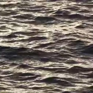
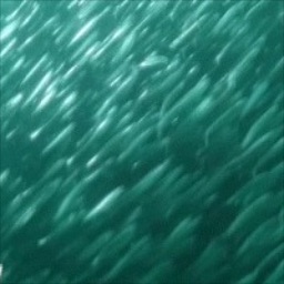
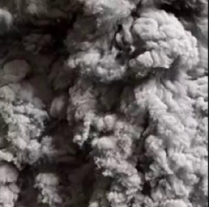
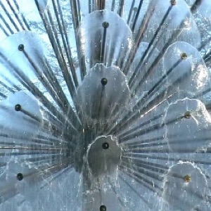
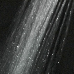
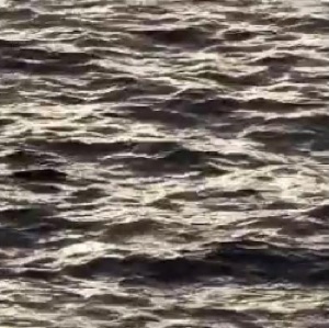
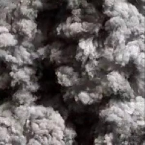
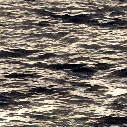
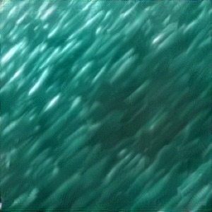
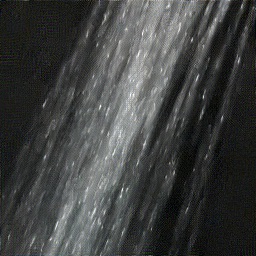
Fig. 1: This figure gives six representative dynamic texture examples (one column per texture), where the left three are homogeneous textures while the right three are structured textures. The first row shows one frame of reference dynamic texture video, the second row shows synthesized results obtained by the baseline model, and the third row shows results obtained using our model.

The first limitation is the existing model fails for texture examples that have the long-range spatial correlation. Some examples are shown in the 4th, 5th and 6th columns of Fig. 1. As discussed in previous work [6, 7], this drawback is attributed to the fact that the current loss function (i.e., the Gram loss) is not efficient in characterizing the long-range spatial correlation. It is shown by experiments that the Gram loss can provide excellent performance in capturing local image properties such as texture patterns. Yet, it cannot handle long-range image information well since such information is discarded in the modeling process. Actually, we observe that existing solutions fail to provide satisfactory performance in synthesizing dynamic textures with long-range as well as mid-range correlations.

The second drawback is that the current model can generate textures with monotonous motion, i.e. relatively smooth motion between adjacent frames. In other words, the generated samples do not have diversified dynamics. Sometimes, they even appear to be periodic. This is because that previous models primarily focus on dynamics between adjacent frames, but ignore motion in a longer period. For example, Funke et al. [7] used the correlation matrix between frames to represent the motion information, and Tesfaldet et al. [6] adopted a network branch for optical flow prediction to learn dynamics. This shortcoming yields visible distortion to the perceptual quality of synthesized results.

Being motivated by the above two drawbacks, we propose a new solution to address them in this paper. First, we incorporate a new loss term, called the Shifted Gram loss, to capture the structural and long-range correlation of the reference texture video. Second, we introduce a frame sampling strategy to exploit long-period motion across multiple frames. The solution is implemented using an enhanced two-branch convolutional neural network. It can synthesize dynamic texture with long-range spatial and temporal correlations. As shown in Fig. 1, the proposed method could take care of both homogeneous and structured texture patterns well. Extensive experimental results will be given to show the superiority of the proposed method.

2 Related Work

Texture analysis on classification and segmentation has been studied for decades and great success have been made in the past several years [8, 9]. Recently, more research attention has been paid to static texture image synthesis problem, e.g., [10, 11, 12]. Berger and Memisevic [10] used a variation of the Gram loss that takes spatial co-occurrences of local features into account. Zhou et al. [11] proposed a generative adversarial network (GAN) that was trained to double the spatial extent of texture blocks extracted from a specific texture exemplar. Sendik and Cohen-Or [12] introduced a structural energy loss term that captures self-similar and regular characteristics of textures based on correlations among deep features.

However, in spite of these efforts, dynamic texture synthesis remains to be a challenging and non-trivial problem for several reasons. First, even it is possible to capture and maintain the structural information in a single image, it is still difficult to preserve the structural information in an image sequence. Second, there exist more diversified patterns in dynamic textures due to various spatio-temporal arrangement. More analysis with illustrative examples will be elaborated in Sec. 4. To summarize, extending a static texture synthesis model to a dynamic one is not a straightfoward problem, which will be the focus of our current work.

3 Proposed Method

The baseline model to be used in our work is the two-stream CNN proposed by Tesfaldet et al. [6]. In this section, we will briefly introduce the baseline model, including the network structure, the learning method and the synthesis process. Then, we will propose several techniques to address long-range spatial and temporal correlations in the underlying reference texture sequence.

3.1 Baseline Model

The baseline model is constructed from two convolutional networks (CNNs), an appearance stream and a dynamics stream. Such kind of two-stream design enables the model to factorize appearance and dynamics of dynamic texture and proceed with the analysis independently. Similar to previous work on textures synthesis, the networks summarizes an input dynamic texture in terms of a set of activation statistics of filter outputs,and then build a handbook for each texture of interest in a dictionary learning manner.

During the synthesis process, it optimizes a randomly initialized noise pattern such that its spatio-temporal statistics from each stream match those of the input texture. To achieve that, the model conducts Gradient Descent and Back-propagation during the synthesis process, and it optimizes the loss function with respect to each pixel to match the spatio-temporal statistics. Meanwhile, all the parameters from object recognition and optical flow prediction networks are pre-trained and remain fixed during the synthesis process.

Appearance Stream. The design of appearance stream follows the spatial texture model which is first introduced by [13]. We use the same publicly available normalized VGG19 network[14] which is first used by [13]. Previous research has shown that such kind of CNN pre-trained on an object classification task can be very effective at characterizing texture appearance.

To describe the appearance of an input dynamic texture, we first feed each frame of input video into the network, and denote the feature maps at layer $l$ as $F^{l}_{i}\in M_{l}$, where $F^{l}_{i}$ is the $i^{th}$ vectorized feature map of layer $l$, and $M_{l}$ is the number of entrances in each feature map of layer $l$. Then, the pair-wise product of each vectorized feature map, i.e. Gram matrix is defined as

$$G^{l}_{ij}=\frac{1}{M_{l}}\sum^{M_{l}}_{k}{F^{l}_{ik}F^{l}_{jk}}=\frac{1}{M_{l}}F^{l}_{i}\cdot F^{l}_{j},$$ (1)

where $\cdot$ means inner product. Following previous works, we use feature maps at the following five layers: Conv layer 1, Pooling layer 1, Pooling layer 2, Pooling layer 3, Pooling layer 4.

In the synthesis process, we initialize a random noise sequence $\hat{I}$, and then feed them into network to proceed with its Gram matrix representation $\hat{G}$. Then the apparent loss could be defined as

$$\mathcal{L}^{l}_{Appearance}=\frac{1}{M_{l}}\sum_{i,j}(G^{l}_{ij}-\hat{G}^{l}_{ij})^{2}$$ (2)

The final apparent loss is weight sum from all selected layers defined as

$$\mathcal{L}_{Appearance}=\sum_{l}w_{l}\mathcal{L}^{l}_{Appearance}.$$ (3)

Dynamics stream. The dynamic stream follows the baseline model [6] employing a pre-trained optical flow prediction network, which takes each pair of temporally consecutive frames as input. The structure of dynamic stream is described as following. The first layer consists of 32 $3D$ convolution filters of spatial size $11\times 11$. Then, a squaring activation function and $5\times 5$ spatial max-pooling with a stride of one are applied sequentially. Then, a $1\times 1$ convolution layer follows with 64 filters follows. Finally, to remove local contrast dependence, a L1 divisive normalization is applied. To capture dynamic, i.e. texture motion, in multiple scales, a image pyramid is employed, and image at each scale is processed independently and concatenated to get the final feature.

To describe the dynamic of an input dynamic texture, we feed each pair of consecutive frames into the network, and conduct exactly same Gram matrix computing as the appearance stream. Here, we use $D$ to denote Gram matrix in dynamic stream. During the synthesis process, we could have $\hat{D}$ computed from the generated dynamic texture $\hat{I}$. Then the dynamic loss could be defined as

$$\mathcal{L}^{l}_{Dynamic}=\frac{1}{M_{l}}\sum_{i,j}(D^{l}_{ij}-\hat{D}^{l}_{ij})^{2}.$$ (4)

The final apparent loss is weighted sum from all selected layers defined as

$$\mathcal{L}_{Dynamic}=\sum_{l}w_{l}\mathcal{L}^{l}_{Dynamic}.$$ (5)

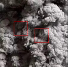
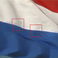
Fig. 2: This figure shows the importance of local feature correlation in structural texture. The red boxes above show a pair of texture patches in the same location. And those patches could be viewed as visualization of the receptive field in a certain layer.

3.2 Proposed Method - I

The effectiveness of Gram matrices could be explained as it captures the coherence across multiple feature maps at a single location. In another word, if we view the pre-trained CNN as a well-designed filter sets, the correlation between responses of different filter sets describe the appearance of texture. And this kind of coherence is so powerful for texture that we could even use a shallow network with random weights to synthesize static texture, even without the help from the complicated pre-trained CNN. And the similar methods have been adopted in many other computer vision topics, like image style transfer and impainting. However, as shown in 1, it still has non-negligible drawbacks.

Form the equation, we could find that the Gram matrices are totally blind to the global arrangement of objects inside each frame of the reference video. Specifically, we could see that it makes pair-wise feature production in each single location and then take the spatial averaging. As a result, all spatial information is erased during the inner product calculation, which makes it fail to capture structural information in a relative large scale. Herein, inspired by [10], we integrate the following shifted Gram matrices to replace the original Gram matrices.

$$\hat{G}^{l}_{ij}=\frac{1}{M_{l}}T(F^{l}_{i})\cdot T(F^{l}_{j}),$$ (6)

where $T$ is a spatial transform operator. By this way, we could further capture the correlation between local feature and feature from its neighborhood. And we could adapt various spatial transform with different angel and aptitude. Gram matrices only make use of correlations between feature maps whereas image structures are represented by the correlations inside each feature map.

The importance and effectiveness of those spatial correlation between local feature and its neighborhood could be illustrated with 2. If the dynamic texture has a homogeneous appearance, the two texture patches will have very weak correlation. For example, in homogeneous texture like smoke, if we fix the left patch in the synthesis process, we could have many possible texture appearance in the location of right patch, as long as it consists with its local neighbor in a natural way. On the contrary, in a structural texture like flag, those two patches in the same location will have a stronger dependency. If we fix one of them, the other one must obey the constraint.

Then, the appearance loss with a spatial transform operator $T$ could be computed accordingly. And we could designed a combination of different $T$ to get a comprehensive appearance loss.

3.3 Proposed Method - II

Fig. 3: This figure shows the importance of middle and long-range motion, Using flag sequence as an example, we can find that most meaningful motion are actually crossing multiple frames. Such kind of long-range motion combines with long-range spatial structure give us a vivid visual effect together.

There two critical requirements to synthesize perceptually natural textures: spatial consistency and temporal consistency. The proposed method in the previous section is designed to render textures when it has long-range structure within each frame. In other words, it handles the non-uniformity in spatial domain. So, a very straightforward extension is that, is there existing non-uniformity in temporal domain? And can the previous model handle that? More specifically, here we use non-uniformity in temporal domain to refer the long-time and non-local motion in dynamic texture.

Actually, this is a quite obvious problem when we try to generalize the model from homogeneous texture to structure texture. First, texture with long-range structure naturally owns more complicated motion patterns with time elapsing. Second, maintaining long-range structures stable and continuous in continuous frames will be much harder comparing with homogeneous texture. Oppositely, the synthesized result from the previous model often looks periodic, which could be a huge drawback and damage the perceptual quality of those synthesized results. Moreover, we also observe the previous model could generate some local motion hopping in continuous frames, which also implies the temporal consistency need to be improved.

In the baseline model, it uses an optical flow prediction network to get features that capture the dynamic between every two consecutive frames. And those features are further utilized in the synthesis process. So, in the previous method, all temporal dynamic in synthesis results is from frame pairs between two consecutive frames, and those temporal dynamic features are further averaged over the whole video. That makes the model only learn the temporal motion/dynamic in a very short time period, and ignore any potential long-range temporal pattern in the reference video.

Here, we employ a simple yet effective approach to encode both short-range motion and long-range motion. We proposed a multi-period frame sampling strategy to modify the dynamic loss. Rather than simply using each consecutive frame pairs, we first set a sampling interval $t$, and then take $i$th frame with $i+t$th frame as a pair to compute the dynamic loss with interval $t$ as follow

$$\mathcal{L}_{Dynamic}(t)=\sum_{i,l}\beta_{l}\mathcal{L}^{l}_{Dynamic}(t;i).$$ (7)

The final dynamic loss is the weighted sum of all selected time intervals

$$\mathcal{L}_{Dynamic}=\sum_{t}\alpha_{t}\mathcal{L}^{l}_{Dynamic}(t).$$ (8)

4 Experiment

In this section, we show our experimental results on both homogeneous and structural dynamic texture video, and then further compare the proposed method with the baseline model. Given their temporal nature, our results are best viewed as videos.

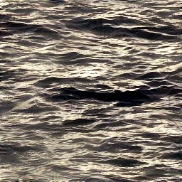
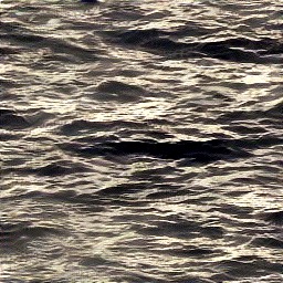
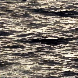
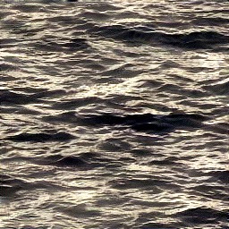
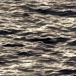
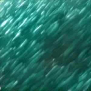
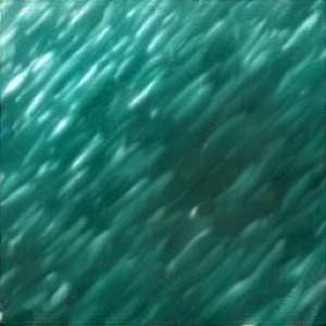
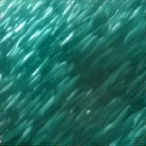
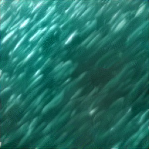
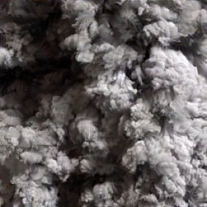
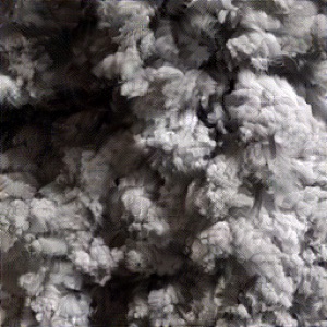
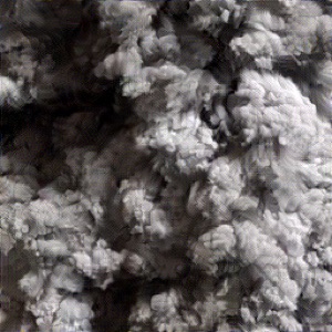
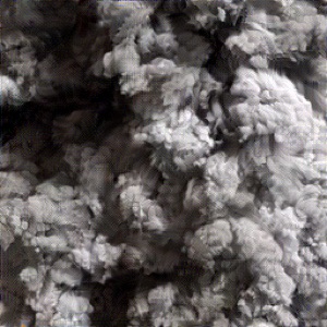
Fig. 4: This figure give several examples of homogeneous dynamic texture frame by frame.

4.1 Experiment Setting

Our two-stream architecture is implemented using TensorFlow. Results were generated using an NVIDIA Titan X GPU and synthesis time ranges between 10 to 30 minutes to generate 8 frames with an image resolution of 256 by 256. To achieve a fair comparison, all dynamic texture samples shown in this paper are selected from DynTex Dataset [15] following the baseline model [6].

Dynamic textures are implicitly defined as the local minimum of this loss function. Textures are generated by optimizing with respect to the pixels of the video. Diversified results could be obtained by initializing the optimization process using I.I.D. Gaussian noise, and the non-convex property of the loss function could also provide extra variations. Consistent with previous works [13, 6], we use L-BFGS [16] optimizer.

For appearance stream, we use Conv layer 1, Pooling layer 1, Pooling layer 2, Pooling layer 3, Pooling layer 4 to compute $\mathcal{L}_{Appearance}$. For proposed technique I, here we use horizontal and vertical transform as our $T$, and the shift distances are set as 8, 16, 32, and 128. For proposed technique II, we choose time interval as 1, 2, and 4. All other settings remain the same as baseline to achieve a fair comparison.

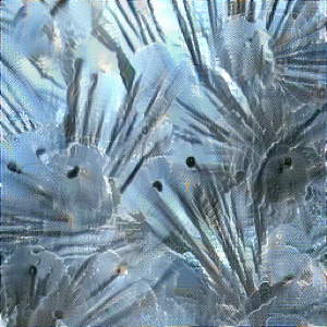
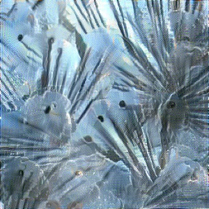
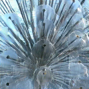
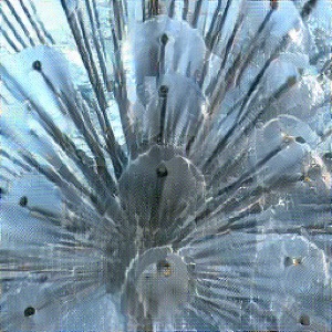
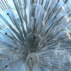
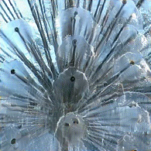
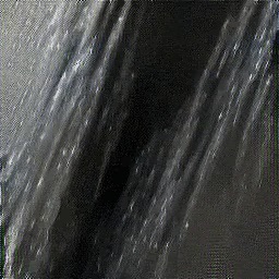
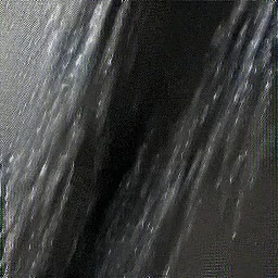
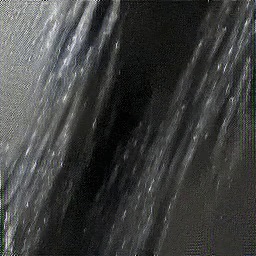
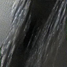
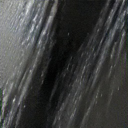
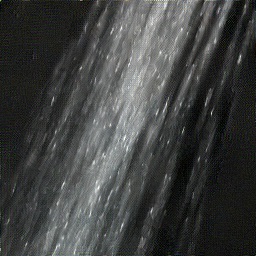
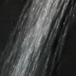
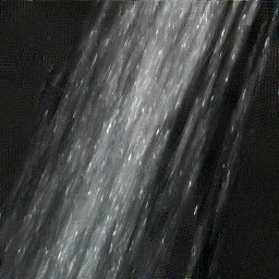
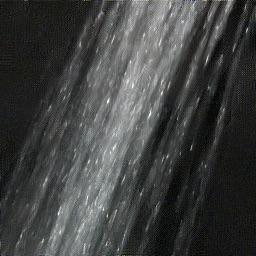
Fig. 5: This figure gives several examples of dynamic textures which contain structural information with long-range correlations.

4.2 Experimental Results

We further conduct experiments on several typical dynamic texture sequence which contain strong structural information. To achieve a fair comparison, here we list synthesized results from both baseline and our model, frame by frame.

Homogeneous Dynamic Texture. We first test our methods on several typical homogeneous dynamic texture sequences. The purpose is to verify that the proposed method could maintain the advantages of baseline model and keep the ability of synthesizing excellent homogeneous dynamic textures. Fig.4 shows some examples of synthesized dynamic texture frame by frame.

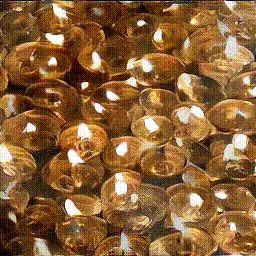
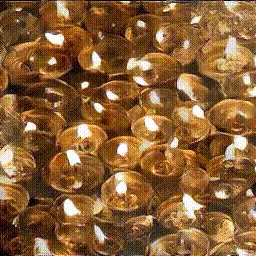
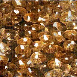
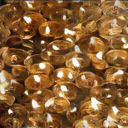
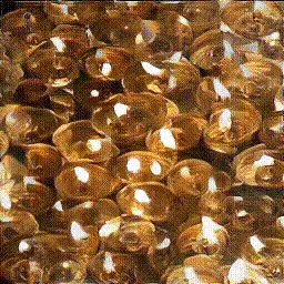
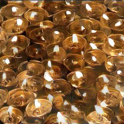
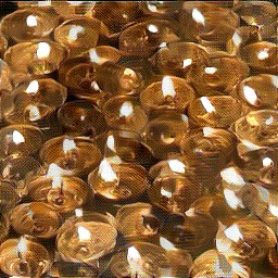
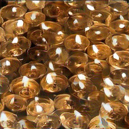
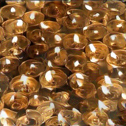
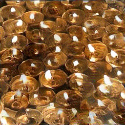
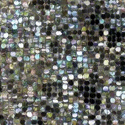
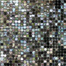
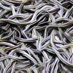
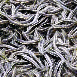
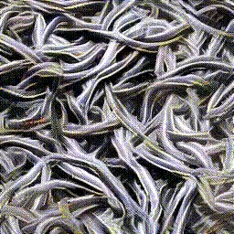
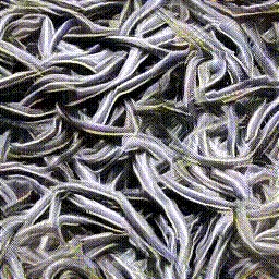
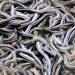
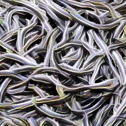
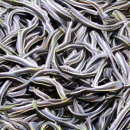
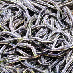
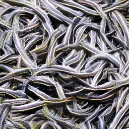
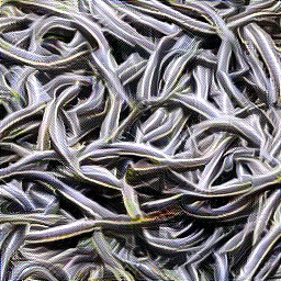
Fig. 6: This figure gives several examples of dynamic texture which contain structural information with middle-range correlations.

Structure with long-range correlation. As for dynamic texture with long-range structure, our proposed method outperforms the baseline model on all these sequences, and several typical exampled are shown in Fig. 5. Noteworthily, proposed techniques work well even all those sequences have quite different forms of long-range correlation. In the flag sequences, the structural information externalizes as the boundary between two colors, which is an irregular curve and across the whole dimension. To make a natural synthesis, the boundary must be sharp and clear in each frame, and also has wavy motion as the other part of the flag. In the fountain sequence, the structural information is shown by the stable fountain skeleton behind the flowing water. Unlike the flag, the fountain sequence requires those edge stable, and any motion will lead to failure results. In the shower sequence, the difficulty is how to teach the model to learn the discrete water trajectory as well as the uniform background. As more results shown on our project page, there are more kinds of different form of long-range correlations in dynamic texture sequences, but our proposed method could handle them in an unified manner.

Structure with middle-range correlation. We also notice that there are a lot of texture in between of homogeneous texture and structural texture. As shown in Fig.6, some kind of dynamic textures have structures which is not global and obvious, but such kind of structures are still critical for perceived quality of our synthesized results. For example, in the candle sequence, we must keep edge of those candles approximated circular. Similarly, we need to keep the snake’s torso natural and smooth in the snake sequence.

Another interesting thing about such kind of sequences, as we point out in previous section, is the results from baseline model show many unexpected sudden local hopping at local structure in consecutive frames. Due to their temporal nature, we recommend to view those results in video form to fully understand this phenomenon.The reason behind those flaws, as we analyzed, is the lack of enough constraint for those local structures leads to discontinuity in the time dimension. By introducing better activation statistics, our model shows better results on such kind of sequences as well.

We have explored proposed techniques thoroughly and found a few limitations which we leave as potential future improvements. First, although dynamic textures are highly self-similar in the spatial domain, the temporal motion in a dynamic texture video is much more complicated(Fig. 2). Second, like most previous models and some works in similar areas, the generated video only has a relatively low resolution. In other words, those generated videos are more like visual effects but not real videos with vivid details. So, there is still a non-neglected distance to generate dynamic textures with better temporal motion in a higher resolution.

5 Conclusion

Two effective techniques for dynamic texture synthesis were presented and proved effective. Compared with the baseline model, the enhanced model could encode coherence of local features as well as the correlation between local feature and its neighbors, and also capture more complicated motion in the time domain. It was shown by extensive experimental results that the proposed method offers state-of-the-art performance.

References

- [1] David J Heeger and Alex P Pentland, “Seeing structure through chaos,” in Proceedings of the IEEE Motion Workshop: Representation and Analysis. IEEE, 1986, pp. 131–136.
- [2] Randal C Nelson and Ramprasad Polana, “Qualitative recognition of motion using temporal texture,” CVGIP: Image understanding, vol. 56, no. 1, pp. 78–89, 1992.
- [3] Gianfranco Doretto, Alessandro Chiuso, Ying Nian Wu, and Stefano Soatto, “Dynamic textures,” International Journal of Computer Vision, vol. 51, no. 2, pp. 91–109, 2003.
- [4] Jianwen Xie, Ruiqi Gao, Zilong Zheng, Song-Chun Zhu, and Ying Nian Wu, “Learning dynamic generator model by alternating back-propagation through time,” arXiv preprint arXiv:1812.10587, 2018.
- [5] Tian Han, Yang Lu, Jiawen Wu, Xianglei Xing, and Ying Nian Wu, “Learning generator networks for dynamic patterns,” in 2019 IEEE Winter Conference on Applications of Computer Vision (WACV). IEEE, 2019, pp. 809–818.
- [6] Matthew Tesfaldet, Marcus A Brubaker, and Konstantinos G Derpanis, “Two-stream convolutional networks for dynamic texture synthesis,” in Proceedings of the IEEE Conference on Computer Vision and Pattern Recognition, 2018, pp. 6703–6712.
- [7] Christina M Funke, Leon A Gatys, Alexander S Ecker, and Matthias Bethge, “Synthesising dynamic textures using convolutional neural networks,” arXiv preprint arXiv:1702.07006, 2017.
- [8] Kaitai Zhang, Hong-Shuo Chen, Ye Wang, Xiangyang Ji, and C-C Jay Kuo, “Texture analysis via hierarchical spatial-spectral correlation (hssc),” in 2019 IEEE International Conference on Image Processing (ICIP). IEEE, 2019, pp. 4419–4423.
- [9] Kaitai Zhang, Hong-Shuo Chen, Xinfeng Zhang, Ye Wang, and C-C Jay Kuo, “A data-centric approach to unsupervised texture segmentation using principle representative patterns,” in ICASSP 2019-2019 IEEE International Conference on Acoustics, Speech and Signal Processing (ICASSP). IEEE, 2019, pp. 1912–1916.
- [10] Guillaume Berger and Roland Memisevic, “Incorporating long-range consistency in cnn-based texture generation,” arXiv preprint arXiv:1606.01286, 2016.
- [11] Yang Zhou, Zhen Zhu, Xiang Bai, Dani Lischinski, Daniel Cohen-Or, and Hui Huang, “Non-stationary texture synthesis by adversarial expansion,” arXiv preprint arXiv:1805.04487, 2018.
- [12] Omry Sendik and Daniel Cohen-Or, “Deep correlations for texture synthesis,” ACM Transactions on Graphics (TOG), vol. 36, no. 5, pp. 161, 2017.
- [13] Leon Gatys, Alexander S Ecker, and Matthias Bethge, “Texture synthesis using convolutional neural networks,” in Advances in neural information processing systems, 2015, pp. 262–270.
- [14] Karen Simonyan and Andrew Zisserman, “Very deep convolutional networks for large-scale image recognition,” arXiv preprint arXiv:1409.1556, 2014.
- [15] Renaud Péteri, Sándor Fazekas, and Mark J Huiskes, “Dyntex: A comprehensive database of dynamic textures,” Pattern Recognition Letters, vol. 31, no. 12, pp. 1627–1632, 2010.
- [16] Dong C Liu and Jorge Nocedal, “On the limited memory bfgs method for large scale optimization,” Mathematical programming, vol. 45, no. 1-3, pp. 503–528, 1989.