Deterministic quantum one-time pad via Fibonacci anyons

Abstract

Anyonic states, which are topologically robust because of their peculiar structure of Hilbert space, have important applications in quantum computing and quantum communication. Here we investigate the capacity of the deterministic quantum one-time pad (DQOTP) that uses Fibonacci anyons as an information carrier. We find that the Fibonacci particle-antiparticle pair produced from vacuum can be used to asymptotically send $2\log_{2}d_{\tau}$ bits of classical information ($d_{\tau}$ is the quantum dimension of a Fibonacci anyon $\tau$), which equals anyonic mutual information of the pair. Furthermore, by studying the DQOTP via a parameterized state of six Fibonacci anyons with trivial total charge, we give the analytical results of the maximum number of messages that can be sent for different parameters, which is a step function with every step corresponding to a regular simplex from the viewpoint of geometry. The results for the maximum number of messages sent by the DQOTP can be explained by anyonic accessible information.

I Introduction

In quantum communication the superdense coding [1, 2] shows that channel capacity can be increased by the entanglement between Alice (sender) and Bob (receiver). Afterwards Schumacher and Westmoreland [3] presented a quantum protocol called the quantum one-time pad, which can be seen as a generalization of the superdense coding. In the protocol, Alice and Bob share a quantum state $\rho^{AB}$. The classical message, which Alice wants to send to Bob, is encoded by Alice’s quantum operations on her subsystem. Then Alice sends her subsystem to Bob, and Bob performs a quantum measurement to decode the message. To ensure security, Alice’s operations must meet some conditions. Reference [3] showed that the maximum amount of information transformed securely equals the quantum mutual information of the initial state $\rho^{AB}$. This quantum protocol has drawn much attention and has been further studied [4, 5].

Recently, a kind of quantum state named the anyonic state in a two-dimensional topologically ordered phase [6, 7, 8, 9] has attracted the attention of theorists and experimentalists for its potential in building a topological fault-tolerant quantum computer [10]. Moreover, the information encoded in anyons presents some unusual properties. In particular, when a two-dimensional gapped system stays in a topologically ordered phase, the entanglement entropy of its ground state contains a sub-leading constant term in addition to the leading area-law term [11, 12]. This motivates us to consider the question of whether the exotic properties of anyonic systems could lead to unexpected results in the field of quantum communication.

However, the answer to this question is not straightforward. Compared with the Hilbert space of the conventional quantum system, the Hilbert space of the anyonic system possesses remarkable properties. The Hilbert space of an anyonic system is decomposed into a direct sum of sectors

$$\mathcal{H}=\oplus_{q}\mathcal{H}_{q},$$ (1)

where $q$ is the charge of a sector. If a local anyonic system is well isolated from the other anyons, then its charge $q$ will be conserved under any local physical process. This property is called the superselection rule for an anyonic system [13], which lays the foundation for its application in fault-tolerant quantum computing. Moreover, the Hilbert space of two local anyonic subsystems is not the direct product of the Hilbert spaces of the two subsystems but a direct sum of some factorizable Hilbert spaces. To be specific, the Hilbert space of an anyonic system with the total charge $c$ containing two local subsystems $A$ and $B$ is

$$\mathcal{H}^{c}_{AB}=\bigoplus_{a,b}\mathcal{H}_{A}^{a}\otimes\mathcal{H}_{B}^{b}\otimes V_{ab}^{c},$$ (2)

where $a$ ($b$) is the total charge of subsystem $A$ ($B$) and $V_{ab}^{c}$ is the fusion Hilbert space associated with the process that two anyons with charges $a$ and $b$ fuse into an anyon with charge $c$ [13]. Therefore, our existing concepts and methods in quantum information theory [14] cannot be directly applied in anyonic systems.

In this paper, we study the deterministic quantum one-time pad, where Bob can deterministically distinguish different messages, in anyonic systems. For simplicity we consider the Fibonacci anyon model [15], the simplest one that can be used for universal topological quantum computation. We find that the Fibonacci particle-antiparticle pair produced from vacuum, which was used for anyonic teleportation [16],

$$\ket{\mathcal{B}}=\ket{\tau,\tau;1},$$ (3)

for which the notation will be introduced in Sec. III, can be used to transmit messages securely in the asymptotic sense. We will show that the channel capacity of the state $\ket{\mathcal{B}}$ in the quantum one-time pad equals the state’s anyonic mutual information based on anyonic von Neumann entropy [17], which is a direct generalization of the corresponding result in Ref. [3]. Further more, we study the deterministic quantum one-time pad via a parameterized state of six Fibonacci anyons with the total charge being vacuum, which includes the above three copies of $\ket{\mathcal{B}}$ as a special case. To our surprise, although the three copies of $\ket{\mathcal{B}}$ have the maximum anyonic mutual information, it is not the state that sends the maximum number of messages. In the end, we conclude by giving a summary and an outlook.

II Preliminaries

Before studying the deterministic quantum one-time pad via Fibonacci anyons, we will introduce the necessary concepts of the quantum one-time pad and the Fibonacci anyon model.

II.1 Quantum one-time pad

In the one-time pad encryption scheme [18, 14], Alice and Bob share privately a random key, i.e., a random string of bits. For every message, Alice encrypts her message by adding the message and the key using bitwise addition modulo $2$ and sends the encrypted message to Bob publicly. Then Bob decrypts the encrypted message by subtracting the shared key to invert the encoding. The message is secure if every random key is secure and used only once.

The quantum one-time pad proposed by Schumacher and Westmoreland [3] is a quantum analog of the one-time pad, where a random key shared between Alice and Bob is replaced by a quantum state $\rho^{AB}$. In this quantum protocol, Alice and Bob initially share a quantum state $\rho^{AB}$. Alice encrypts her message $\alpha$ by performing a quantum operation ${\mathcal{E}}^{A}_{\alpha}\otimes I^{B}$ on the state $\rho^{AB},$ and sends her subsystem $A$ to Bob publicly. Then Bob decrypts the message $\alpha$ by performing a quantum measurement on the whole system in the state $\sigma^{AB}_{\alpha}=\mathcal{E}^{A}_{\alpha}\otimes I^{B}(\rho^{AB})$. It should be noted that the subsystem $A$ may also be available to an eavesdropper named Eve. To ensure the security, Alice’s operation must meet the security condition ${\mathcal{E}}^{A}_{\alpha}(\rho^{A})=\rho^{A}$ for every $\alpha$, with $\rho^{A}$ being the reduced states of $\rho^{AB}$.

In general, Alice’s task in the quantum one-time pad is to send a classical message $\alpha$ from some message set with probability $p_{\alpha}$. Then Bob’s accessible information is upper bounded by the Holevo bound [14]

$$\mathcal{X}(\sigma^{AB})=S(\sigma^{AB})-\sum_{\alpha}p_{\alpha}S(\sigma_{\alpha}^{AB}),$$ (4)

where $S(\eta)$ is the von Neumann entropy of the state $\eta$, i.e., $S(\eta)\equiv-\Tr(\eta\log_{2}\eta)$. In Ref. [3], this maximum amount of information transformed securely was proved to equal the quantum mutual information of the initial state $\rho^{AB}$ asymptotically

$$I(\rho^{AB})=S(\rho^{A})+S(\rho^{B})-S(\rho^{AB}).$$ (5)

For simplicity and convenience, we will restrict ourselves to a specific type of quantum one-time pad protocol called the deterministic quantum one-time pad (DQOTP), where the following three assumptions are assumed. First, the key state $\rho^{AB}$ is a pure state $|\psi\rangle$. Second, all of Alice’s encoding operations $\{\mathcal{E}_{\alpha}^{A}\}$ are unitary transformations $\{U_{\alpha}^{A}\}$. Third, Bob can distinguish different messages $\{\alpha\}$ by making a quantum measurement, which implies that the states $\{U_{\alpha}^{A}\otimes I^{B}|\psi\rangle\}$ are orthogonal to each other.

II.2 Fibonacci anyon model

In the Fibonacci anyon model, there are two species of anyons: $1$ and $\tau$, where $1$ denotes the vacuum and $\tau$ denotes the Fibonacci anyon. The species of anyons are also called topological charges. These anynos can be combined or split according to the following fusion rules:

$$1\times\tau =\tau,$$

$$\tau\times 1 =\tau,$$

$$\tau\times\tau =1+\tau.$$ (6)

For example, the fusion rule $\tau\times\tau=1+\tau$ means there are two possible fusion results $1$ and $\tau$ when two $\tau$s are fused. It also means charge $1$ ($\tau$) can be split into two $\tau$s.

The quantum state of the Fibonacci anyon model is defined by the above fusion rules. For example, the state of $2$ $\tau$s fusing into the vacuum is given by $\bra{\tau,\tau;1}$, the state of the vacuum splitting into $2$ $\tau$s is given by $\ket{\tau,\tau;1}$. When there are more anyons in the system, we need to specify the order of fusion or splitting.

In the Fibonacci anyon model, a basic unitary transformation $R_{\tau\tau}$ is realized by braiding two $\tau$s. By performing a series of such braidings, the Fibonacci anyon model was shown to be able to realize universal topological quantum computing [19, 20, 21].

For completeness, we give more technical details of the description of the Hilbert space of the Fibonacci anyon model in the Appendix.

III Anyonic deterministic one-time pad

In this section, we aim to study the deterministic quantum one-time pad via the Fibonacci anyons. First, we introduce the basic framework for the deterministic quantum one-time pad. Second, we obtain the average maximal information in the deterministic quantum one-time pad via Fibonacci Bell states in the asymptotic limit. Third, we obtain the maximal information in the deterministic quantum one-time pad via a parameterized state of six Fibonacci anyons.

III.1 Deterministic quantum one-time pad protocol

Now we are ready to state the protocol of DQOTP by using the Fibonacci anyonic state $|\psi\rangle$ of $2n$ $\tau$’s with trivial total charge, where the $n$ $\tau$’s on the left side are owned by Alice, and the $n$ $\tau$’s on the right side are owned by Bob. Alice performs a unitary transformation $U^{A}_{\alpha}$ on her $n$ $\tau$’s to encode a message $\alpha$. In particular, we require that the message $\alpha$ is secure before Bob receives Alice’s $n$ $\tau$’s, which requires that Alice’s local state is invariant under the unitary transformation, i.e.,

$$U^{A}_{\alpha}\tilde{\rho}^{A}U^{A\dagger}_{\alpha}=\tilde{\rho}^{A},$$ (7)

where Alice’s local state $\tilde{\rho}^{A}=\tilde{\rm Tr}[\ket{\psi}\bra{\psi}]$. Then she sends her $n$ $\tau$’s to Bob such that Bob can make a measurement on the $2n$ $\tau$’s to decode the message $\alpha$. Here we require that Bob can distinguish different messages from Alice deterministically, i.e., the different unitary transformations satisfying the orthogonal condition

$$\bra{\psi}U^{A\dagger}_{\alpha}U^{A}_{\alpha^{\prime}}\ket{\psi}=0$$ (8)

for any different messages $\alpha$ and $\alpha^{\prime}$. Denote the set of unitary transformations satisfying Eqs. (7) and (8) as $\mathcal{U}^{A}=\{U^{A}_{\alpha}\}$. Since each $U^{A}_{\alpha}\in\mathcal{U}^{A}$ represents one distinguishable message for Bob, the cardinality of $\mathcal{U}^{A}$, denoted as $\absolutevalue{\mathcal{U}^{A}}$, equals the number of such messages sent from Alice to Bob. The central problem in the DQOTP is to find out the maximum number of messages from Alice that Bob can distinguish deterministically. In other words, we shall maximize the cardinality $\absolutevalue{\mathcal{U}^{A}}$, i.e.,

$$\max\absolutevalue{\mathcal{U}^{A}}\equiv N_{m}(|\psi\rangle).$$ (9)

III.2 DQOTP via anyonic Bell states

As we know, the Bell state is of great importance in superdense coding, which is used to send $2$ bits of classical information by sending one qubit. Then it is natural to ask which state in the Fibonacci anyon system plays a role similar to the Bell state in the qubit system. A reasonable candidate for a Bell state in the Fibonacci anyon system [16] is the state of $2$ $\tau$’s from vacuum

$$\ket{\mathcal{B}}=\ket{\tau,\tau;1}.$$ (10)

Then Alice and Bob each have one anyon, and their reduced states are $\tilde{\rho}_{A}=\tilde{\rho}_{B}=\frac{1}{d_{\tau}}\ket{\tau,1;\tau}\bra{\tau,1;\tau}$, which can be obtained by using the quantum trace and $F$ matrix defined in the Appendix. The anyonic mutual information for the state $|\mathcal{B}\rangle$ is $\tilde{\mathcal{I}}(|\mathcal{B}\rangle)=2\log_{2}d_{\tau}$, where the anyonic mutual information for the state $\tilde{\rho}^{AB}$ is defined by

$$\tilde{\mathcal{I}}(\rho^{AB})\equiv\tilde{S}(\tilde{\rho}^{A})+\tilde{S}(\tilde{\rho}^{B})-\tilde{S}(\tilde{\rho}^{AB}),$$ (11)

where $\tilde{S}(\tilde{\rho})=-\tilde{\rm Tr}[\tilde{\rho}{\rm log}_{2}\tilde{\rho}]$ is the anyonic von-Neumann entropy [17] and the quantum trace $\tilde{\rm Tr}$ is defined by Eq. (49). Thus we expect that the anyonic state $|\mathcal{B}\rangle$ can be used to send $2\log_{2}d_{\tau}$ bits of classical information from Alice and Bob in the anyonic DQOTP. However, Alice has only one $\tau$, and she can not perform any unitary transformation by braiding, which implies that she can not send classical information in DQOTP, i.e., $N_{m}(|\mathcal{B}\rangle)=0$.

How do we reconcile the above paradox? We turn to study DQOTP by using the $n$ copies of the state $|\mathcal{B}\rangle$ shared between Alice and Bob

$$\ket{\mathcal{B}}^{\otimes n} =\ket{\tau,\tau;1}^{\otimes n}$$

$$=\left(\frac{1}{d_{\tau}}\right)^{\frac{n}{2}}\leavevmode\hbox to114.21pt{\vbox to85.66pt{\text{[drawing]}}}, n \tau n \tau$$ (12)

where the first $n$ $\tau$’s from left to right belong to Alice, and the rest belongs to Bob. Here, we utilize the diagrammatic representation of the anyonic state (see the Appendix). We aim to show that the state $|\mathcal{B}\rangle$ per copy in the asymptotic limit can send $2\log_{2}d_{\tau}$ bits of classical information in the anyonic DQOTP, i.e.,

$$\lim_{n\to\infty}\frac{\log_{2}N_{m}(|\mathcal{B}\rangle^{\otimes n})}{n}=\tilde{\mathcal{I}}(|\mathcal{B}\rangle)=2\log_{2}d_{\tau}.$$ (13)

We prove one of our main results, Eq. (13), as follows. By using the basis transformation named the $F$ move [17]

$$= \sum_{b}\left[F^{a_{2}a_{1}\overline{a}_{1}}_{a_{2}}\right]_{1b}\leavevmode\hbox to128.42pt{\vbox to71.45pt{\text{[drawing]}}}, a_{1} a_{2} b \overline{b} \overline{a}_{2} \overline{a}_{1} a_{1} a_{2} b \overline{b} \overline{a}_{2} \overline{a}_{1}$$ (14)

where the coefficient $\left[F^{a_{2}a_{1}\overline{a}_{1}}_{a_{2}}\right]_{1b}=\sqrt{d_{b}/(d_{a_{1}}d_{a_{2}})}$, we can perform the Schmidt decomposition on the state $\ket{\mathcal{B}}^{\otimes n}$,

$$\ket{\mathcal{B}}^{\otimes n}$$

$$= \left(\frac{1}{d_{\tau}}\right)^{\frac{n}{2}}\sum_{i=1}^{F(n-1)}\ket{i;n\;\tau\text{s};1}_{A}\otimes\ket{i;n\;\tau\text{s};1}_{B}$$

$$+\left(\frac{1}{d_{\tau}}\right)^{\frac{n-1}{2}}\sum_{j=1}^{F(n)}\ket{j;n\;\tau\text{s};\tau}_{A}\otimes\ket{j;n\;\tau\text{s};\tau}_{B}\otimes\ket{\tau,\tau;1},$$ (15)

where $\ket{i;n\;\tau\text{s};a}_{A}$ ($a\in\{1,\tau\}$) is the $i$th orthonormal basis vector of $n$ $\tau$’s in subsystem $A$ with total charge $a$, the diagrammatic representations for $\ket{i;n\;\tau\text{s};a}_{A}$ and $\ket{i;n\;\tau\text{s};a}_{B}$ are mirror symmetric, and

$$F(n)=\frac{d_{\tau}^{n}-(-d_{\tau})^{-n}}{2d_{\tau}-1}$$ (16)

is Binet’s formula [22] which gives the $n$th term in the Fibonacci sequence, e.g., $F(0)=0$, $F(1)=1$, $F(2)=1$, and $F(3)=2$. Thus, the local state of Alice can be written as

$$\tilde{\rho}_{n}^{A}=\begin{pmatrix}\left(\frac{1}{d_{\tau}}\right)^{n}I^{1}_{F(n-1)}&0\\ 0&\left(\frac{1}{d_{\tau}}\right)^{n-1}\frac{1}{d_{\tau}}I^{\tau}_{F(n)}\end{pmatrix},$$ (17)

where $I^{a}_{d}$ $(a\in\{1,\tau\})$ is the $d\times d$ identity anyonic matrix of space of $n$ $\tau$’s with total charge $a$. Note that the state $\tilde{\rho}^{A}_{n}$ can also be written as $\frac{1}{d_{\tau}^{n}}I_{n\tau}$, where $I_{n\tau}$ is the identity matrix of the anyonic Hilbert space of $n$ $\tau$’s.

Now the superselection rule implies that any unitary operator $U^{A}_{\alpha}$ encoding the message $\alpha$ can be decomposed into a direct sum of two sectors,

$$U^{A}_{\alpha}=\begin{pmatrix}U_{\alpha}^{1}&0\\ 0&U_{\alpha}^{\tau}\\ \end{pmatrix},$$ (18)

where $U_{\alpha}^{1}$ ($U_{\alpha}^{\tau}$) is the unitary operator living in sector $1$ (sector $\tau$) of operator $U^{A}_{\alpha}$, which meet the security conditions (7) naturally. Because any two states in $\{U_{\alpha}^{A}|\mathcal{B}\rangle^{\otimes n}\}$ are orthogonal (8), the cardinality of $\mathcal{U}^{A}$ is not more than the dimension of the Hilbert space $V_{1}^{2n\tau}$, i.e.,

$$N_{m}(|\mathcal{B}\rangle^{\otimes n})\leq F(n-1)^{2}+F(n)^{2}.$$ (19)

The orthogonal condition (8) can be expressed further as $\forall$ different messages $\alpha$ and $\alpha^{\prime}$,

$$\tilde{\rm Tr}\left[U^{1\dagger}_{\alpha}U^{1}_{\alpha^{\prime}}\right]+\tilde{\rm Tr}\left[U^{\tau\dagger}_{\alpha}U^{\tau}_{\alpha^{\prime}}\right]=0.$$ (20)

Then we can construct one $\mathcal{U}^{A}$, denoted by $\mathcal{U}_{L}^{A}$, that satisfies

$$\tilde{\rm Tr}\left[U^{1\dagger}_{\alpha}U^{1}_{\alpha^{\prime}}\right]=\tilde{\rm Tr}\left[U^{\tau\dagger}_{\alpha}U^{\tau}_{\alpha^{\prime}}\right]=0.$$ (21)

Thus, we can find out $\{U^{1}_{\alpha}\}$ and $\{U^{\tau}_{\alpha}\}$ respectively. It is instructive to consider the DQOTP for the state

$$|\phi^{1}\rangle=\frac{1}{\sqrt{F(n-1)}}\sum_{i=1}^{F(n-1)}\ket{i;n\;\tau^{\prime}\text{s};1}_{A}\otimes\ket{i;n\;\tau^{\prime}\text{s};1}_{B}.$$ (22)

Obviously, $\{U_{\alpha}^{1}\}$ satisfying Eq. (21) is the set of unitary transformations encoding messages $\mathcal{U}^{A}_{L1}$. In this subspace, the problem is reduced to the traditional superdense coding for the maximally entangled state in the $F(n-1)$ dimensional Hilbert space. Thus we can send $F(n-1)^{2}$ messages from Alice to Bob, which implies that the cardinality $\absolutevalue{\mathcal{U}^{A}_{L1}}=F(n-1)^{2}$. Similarly for $\mathcal{U}^{A}_{L\tau}=\{U_{\alpha}^{\tau}\}$, the cardinality $\absolutevalue{\mathcal{U}^{A}_{L\tau}}=F(n)^{2}$. Because $\absolutevalue{\mathcal{U}^{A}_{L1}}\leq\absolutevalue{\mathcal{U}^{A}_{L\tau}}$, we can always take $\absolutevalue{\mathcal{U}^{A}_{L1}}$ elements from $\mathcal{U}^{A}_{L1}$ and $\mathcal{U}^{A}_{L\tau}$ to construct the set $\mathcal{U}^{A}_{L}$, which implies that $\absolutevalue{\mathcal{U}^{A}_{L}}=F(n-1)^{2}$. Thus we obtain

$$N_{m}(|\mathcal{B}\rangle^{\otimes n})\geq\absolutevalue{\mathcal{U}^{A}_{L}}=F(n-1)^{2}.$$ (23)

Then we have the inequality

$$F(n-1)^{2}\leq N_{m}(|\mathcal{B}\rangle^{\otimes n})\leq F(n-1)^{2}+F(n)^{2}.$$ (24)

By using Binet’s formula [see Eq. (16)] we obtain

$$\lim_{n\to\infty}\frac{\log_{2}N_{m}(|\mathcal{B}\rangle^{\otimes n})}{n}=2{\rm log}_{2}d_{\tau},$$ (25)

which completes the proof of Eq. (13).

The main result in Eq. (13) reconciles the paradox discussed: Although a single copy of the anyonic Bell state $|\mathcal{B}\rangle$ can not be used to send any classical information in the DQOTP, one copy in the ensemble of the anyonic Bell states can send $2\log_{2}d_{\tau}$ bits of classical information, which is equal to the anyonic mutual information of an anyonic Bell state. Thus the DQOTP protocol gives an operational meaning to anyonic mutual information and in a sense proves the reliability of the definition of the anyonic entropy. Since the amount of information relates only to the quantum dimension $d_{\tau}$ of Fibonacci anyons, only non-Abelian anyons contain this kind of information.

III.3 DQOTP via a parameterized state of six Fibonacci anyons

Although the anyonic Bell state $|\mathcal{B}\rangle$ plays an important role in the anyonic DQOTP, it is necessary to study this quantum protocol with a more general anyonic state. In this section we consider the following parameterized states of six Fibonacci anyons in the trivial sector

$$|\mathcal{G}(p)\rangle$$

$$= \sqrt{p}\ket{\tau,\tau,\tau;1}_{A}\otimes\ket{\tau,\tau,\tau;1}_{B}$$

$$+\sqrt{\frac{1-p}{2}}\sum_{j=1}^{2}\ket{j;\tau,\tau,\tau;\tau}_{A}\otimes\ket{j;\tau,\tau,\tau;\tau}_{B}\otimes\ket{\tau,\tau;1},$$ (26)

where $p\in\left[0,1\right]$. Note that when $p=1/d_{\tau}^{3}$ the above state equals three copies of the anyonic Bell state $|\mathcal{B}\rangle$, i.e., $|\mathcal{G}(1/d_{\tau}^{3})\rangle=|\mathcal{B}\rangle^{\otimes 3}$. And it can be shown that the state $|\mathcal{B}\rangle^{\otimes 3}$ is the state with maximal mutual information among all states $|\mathcal{G}(p)\rangle$.

We aim to show that the maximal amount of information through DQOTP via the state $|\mathcal{G}(p)\rangle$ is

$$N_{m}(|\mathcal{G}(p)\rangle)=\begin{cases}5&\text{ if }p=\frac{1}{5},\\ 4&\text{ if }0\leq p<\frac{1}{5}\text{ and }\frac{1}{5}<p\leq\frac{1}{4},\\ 3&\text{ if }\frac{1}{4}<p\leq\frac{1}{3},\\ 2&\text{ if }\frac{1}{3}<p\leq\frac{1}{2},\\ 1&\text{ if }\frac{1}{2}<p\leq 1,\end{cases}$$ (27)

which is demonstrated in Fig. 1. From Eq. (27), we find that the state $|\mathcal{G}(1/5)\rangle$ that can be used to send the maximal amount of information is not the maximum entangled state, i.e., three copies of the anyonic Bell state $|\mathcal{B}\rangle^{\otimes 3}$.

Figure 1: The maximum amount of information $N_{m}(|\mathcal{G}(p)\rangle)$ transmitted deterministically from Alice to Bob through the state $\ket{\mathcal{G}(p)}$ for different $p$.

We prove Eq. (27) as follows. Note that Alice’s local state is

$$\tilde{\rho}^{A}(p)=\begin{pmatrix}p&0&0\\ 0&\frac{1-p}{2}\frac{1}{d_{\tau}}&0\\ 0&0&\frac{1-p}{2}\frac{1}{d_{\tau}}\end{pmatrix}.$$ (28)

Following Eq. (7), the unitary operator that Alice uses to encode message $\alpha$ can be written as

$$U_{\alpha}^{A}=\begin{pmatrix}1&0&0\\ 0&a_{\alpha}+ib_{\alpha}&c_{\alpha}+id_{\alpha}\\ 0&-c_{\alpha}+id_{\alpha}&a_{\alpha}-id_{\alpha}\\ \end{pmatrix},$$ (29)

where the real numbers $a_{\alpha},b_{\alpha},c_{\alpha}$, and $d_{\alpha}$ are functions of $p$ satisfying $a_{\alpha}^{2}+b_{\alpha}^{2}+c_{\alpha}^{2}+d_{\alpha}^{2}=1$. From the viewpoint of geometry, each operator $U_{\alpha}^{A}$ can be represented by a unit vector $\vec{v}_{\alpha}=(a_{\alpha},b_{\alpha},c_{\alpha},d_{\alpha})$ in four-dimensional Euclidean space $\mathbb{E}^{4}$. Now the orthogonal condition (8) becomes the following inner-product relation in $\mathbb{E}^{4}$:

$$\vec{v}_{\alpha}\cdot\vec{v}_{\alpha^{\prime}}=-\frac{p}{1-p}.$$ (30)

To obtain the maximal number of messages $N_{m}(|\mathcal{G}(p)\rangle)$ in the anyonic DQOTP, we determine the maximal number of unit vectors $\{\vec{v}_{\alpha}\}$ by solving Eq. (30), which equals $N_{m}(|\mathcal{G}(p)\rangle)$. Without loss of generality, we can always take the first element $U^{A}_{1}$ in the set $\mathcal{U}^{A}$, which is the $3\times 3$ identity operator, which implies that $\vec{v}_{1}=(1,0,0,0)$. Because the absolute value of the inner product of any two unit vectors is not more than $1$, Eq. (30) requires that $p\leq\frac{1}{2}$. This implies that when $p>\frac{1}{2}$, no other vector except $\vec{v}_{1}$ exists such that Eq. (30) is satisfied. Thus we find that if $\frac{1}{2}<p\leq 1$, then $N_{m}(|\mathcal{G}(p)\rangle)=1$.

Since the inner product of any other unit vector and the identity $\vec{v}_{1}$ equals $-\frac{p}{1-p}$, then $\forall\alpha\neq 1$ the unit vector

$$\vec{v}_{\alpha}=(-\frac{p}{1-p},b_{\alpha},c_{\alpha},d_{\alpha}),$$ (31)

with $p\in[0,1/2]$. When $p=\frac{1}{2}$, a unique vector $\vec{v}_{2}=(-1,0,0,0)$ exists, which implies that $N_{m}(|\mathcal{G}(\frac{1}{2})\rangle)=2$.

When $0\leq p<1/2$, $\forall\alpha\neq 1$, we introduce a unit vector in three-dimensional Euclidean space $\mathbb{E}_{3}$ by

$$\vec{w}_{\alpha}=\frac{1-p}{\sqrt{1-2p}}(b_{\alpha},c_{\alpha},d_{\alpha}).$$ (32)

Without loss of generality, we can take $\vec{w}_{2}=(1,0,0)$. For any $\alpha\neq 1$ and $\alpha^{\prime}\neq 1$, the inner-product relation (30) becomes

$$\vec{w}_{\alpha}\cdot\vec{w}_{\alpha^{\prime}}=-\frac{p}{1-2p}.$$ (33)

Since the absolute value of the above inner product is not more than $1$, we have $p\leq\frac{1}{3}$. In other words, when $\frac{1}{3}<p<\frac{1}{2}$, only $\vec{w}_{2}$ exists such that Eq. (33) is satisfied, and $N_{m}(|\mathcal{G}(p)\rangle)=2$.

When $p=\frac{1}{3}$, Eq. (33) becomes $\forall\alpha>2$, $\vec{w}_{2}\cdot\vec{w}_{\alpha}=-1$, i.e., a unique unit vector $\vec{w}_{3}=(-1,0,0)$ exists. Thus, $N_{m}(|\mathcal{G}(\frac{1}{3})\rangle)=3$.

When $0\leq p<1/3$, $\forall\alpha>2$, we introduce a unit vector in two-dimensional Euclidean space $\mathbb{E}_{2}$ by

$$\vec{x}_{\alpha}=\sqrt{\frac{(1-p)(1-2p)}{1-3p}}(c_{\alpha},d_{\alpha}).$$ (34)

Without loss of generality, we can take $\vec{x}_{3}=(1,0)$. For any $\alpha>2$ and $\alpha^{\prime}>2$, the inner-product relation (33) becomes

$$\vec{x}_{\alpha}\cdot\vec{x}_{\alpha^{\prime}}=-\frac{p}{1-3p}.$$ (35)

Since the absolute value of the above inner product is not more than $1$, we have $p\leq\frac{1}{4}$. In other words, when $\frac{1}{4}<p<\frac{1}{3}$, only $\vec{x}_{3}$ exists such that Eq. (35) is satisfied, and $N_{m}(|\mathcal{G}(p)\rangle)=3$.

When $p=\frac{1}{4}$, Eq. (35) becomes $\forall\alpha>3$, $\vec{x}_{3}\cdot\vec{x}_{\alpha}=-1$; that is, a unique unit vector $\vec{x}_{4}=(-1,0)$ exists. Thus, $N_{m}(|\mathcal{G}(\frac{1}{4})\rangle)=4$.

When $0\leq p<1/4$, $\forall\alpha>3$, we introduce a unit vector in two-dimensional Euclidean space $\mathbb{E}_{1}$ by

$$y_{\alpha}=\sqrt{\frac{(1-p)(1-3p)}{1-4p}}d_{\alpha}.$$ (36)

Without loss of generality, we can take $y_{4}=1$. For any $\alpha>3$ and $\alpha^{\prime}>3$, the inner-product relation (35) becomes

$$y_{\alpha}\cdot y_{\alpha^{\prime}}=-\frac{p}{1-4p}.$$ (37)

Since the absolute value of the above inner product is $1$, we have $p=\frac{1}{5}$, and $y_{5}=-1$. Thus, $N_{m}(|\mathcal{G}(\frac{1}{5})\rangle)=5$. In addition, when $0\leq p<\frac{1}{4}$ and $p\neq\frac{1}{5}$, only $y_{4}$ exists such that Eq. (37) is satisfied, and $N_{m}(|\mathcal{G}(p)\rangle)=4$. This completes our proof of Eq. (27).

Note that the above proof is a constructive one. For example, when $p=\frac{1}{5}$, the five vectors $\{\vec{v}_{\alpha}\}$ obtained are given by

$$\vec{v}_{1} =(1,0,0,0),$$

$$\vec{v}_{2} =(-\frac{1}{4},\frac{\sqrt{15}}{4},0,0),$$

$$\vec{v}_{3} =(-\frac{1}{4},-\frac{\sqrt{15}}{12},\frac{\sqrt{30}}{6},0),$$

$$\vec{v}_{4} =(-\frac{1}{4},-\frac{\sqrt{15}}{12},-\frac{\sqrt{30}}{12},\frac{\sqrt{10}}{4}),$$

$$\vec{v}_{5} =(-\frac{1}{4},-\frac{\sqrt{15}}{12},-\frac{\sqrt{30}}{12},-\frac{\sqrt{10}}{4}).$$

In geometry, these five vectors construct a regular 5-cell in four-dimensional Euclidean space $\mathbb{E}^{4}$. Similarly, for any $p$ the vectors $\{\vec{v}_{\alpha}\}$ construct a regular [$N_{m}(|\mathcal{G}(p)\rangle)-1$]-simplex [23]. In other words, the graph corresponds to a regular tetrahedron, a regular triangle, a segment and a trivial point when $N_{m}(|\mathcal{G}(p)\rangle)$ equals $4$, $3$, $2$, and $1$, respectively.

How do we understand the results of $N_{m}(|G(p)\rangle)$ from the information viewpoint? As we know, three copies of the two-qubit Bell state are the maximally entangled state of the six qubits, which can be used to transmit $6$ bits of classical information in the superdense coding. The $6$ bits of information are the maximum amount of the information can be transmitted in the system of six qubits. Thus, we expect that the same thing happened in the anyonic Bell state $|\mathcal{B}\rangle$; that is, three copies of the Bell state $|\mathcal{B}\rangle^{\otimes 3}$ are the state of six $\tau$s that can send the maximum amount information in the anyonic DQOTP. In fact, we find that the state $|\mathcal{B}\rangle^{\otimes 3}$, i.e., $|\mathcal{G}(1/d_{\tau}^{3})\rangle$, is the state with maximal mutual information among all the states $\{|\mathcal{G}(p)\rangle\}$, which seems to support this expectation. By using Eq. (28), we can obtain the mutual information between $A$ and $B$ of the state $|\mathcal{G}(p)\rangle$,

$$\tilde{I}(|\mathcal{G}(p)\rangle)= 2\tilde{S}(\tilde{\rho}^{A}(p))$$

$$= 2\left[-p{\rm log}_{2}p-(1-p){\rm log}_{2}\frac{1-p}{2d_{\tau}}\right].$$ (38)

When $p=1/d_{\tau}^{3}$, $\tilde{I}(|\mathcal{G}(p)\rangle)$ reaches its maximum value. However, our results in Fig. 1 show that this is not the case: the state $|\mathcal{G}(\frac{1}{5})\rangle$ can send five messages, while the state $|\mathcal{B}\rangle^{\otimes 3}$ can send only four messages.

To resolve the above confusion, it is important to realize that the maximum amount of information that Alice can transmit to Bob through the state $\tilde{\rho}^{AB}=\ket{\mathcal{G}(p)}\bra{\mathcal{G}(p)}$ is limited by the Holevo bound [14],

$$\mathcal{X}(\tilde{\rho}^{AB})= \tilde{S}\left(\sum_{\alpha}p_{\alpha}U_{\alpha}^{A}\tilde{\rho}^{AB}U_{\alpha}^{A\dagger}\right)$$

$$-\sum_{\alpha}p_{\alpha}\tilde{S}\left(U_{\alpha}^{A}\tilde{\rho}^{AB}U_{\alpha}^{A\dagger}\right)$$

$$= \tilde{S}\left(\tilde{\sigma}^{AB}\right)-\tilde{S}\left(\tilde{\rho}^{AB}\right)$$

$$= \left(\tilde{S}(\tilde{\rho}^{A})+\tilde{S}(\tilde{\rho}^{B})-\tilde{S}\left(\tilde{\rho}^{AB}\right)\right)$$

$$-\left(\tilde{S}(\tilde{\rho}^{A})+\tilde{S}(\tilde{\rho}^{B})-\tilde{S}\left(\tilde{\sigma}^{AB}\right)\right)$$

$$= \tilde{I}(\tilde{\rho}^{AB})-\tilde{I}(\tilde{\sigma}^{AB})=\log_{2}\absolutevalue{\mathcal{U}^{A}},$$ (39)

where $\tilde{\sigma}^{AB}=\sum_{\alpha}p_{\alpha}U_{\alpha}^{A}\tilde{\rho}^{AB}U_{\alpha}^{A\dagger}$, with $p_{\alpha}=\frac{1}{\absolutevalue{\mathcal{U}^{A}}}$. Equation (III.3) tells us that the maximum information is limited by the difference between the initial and final quantum anyonic mutual information, which equals the cardinality of the set of unitary transformations $\mathcal{U}^{A}$. The results for the accessible information of $|\mathcal{G}(p)\rangle$, the mutual entropy $\tilde{I}(\tilde{\rho}^{AB})$, and $\tilde{I}(\tilde{\sigma}^{AB})$ when the cardinality $\absolutevalue{\mathcal{U}^{A}}$ takes its maximum are shown in Fig. 2, where the base of the logarithm is $2$.

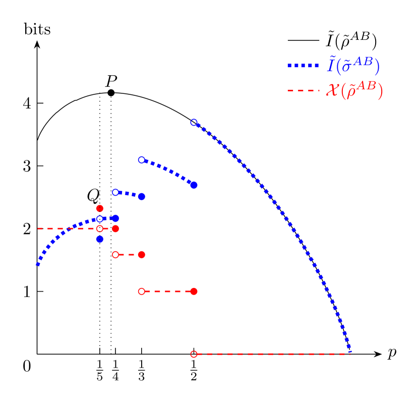
Figure 2: The graph of three functions of $p$: anyonic mutual information $\tilde{I}(\tilde{\rho}^{AB})$ (black solid line), $\tilde{I}(\tilde{\sigma}^{AB})$ (black dotted line), and the Holevo bound $\mathcal{X}(\tilde{\rho}^{AB})$ (red dashed line), which is the difference between $\tilde{I}(\tilde{\rho}^{AB})$ and $\tilde{I}(\tilde{\sigma}^{AB})$. $\tilde{I}(\tilde{\sigma}^{AB})$ and $\mathcal{X}(\tilde{\rho}^{AB})$ are step functions; both are left continuous at points with $p$ coordinates: $1/5$, $1/4$, $1/3$, and $1/2$. $P$ ($Q$) is the extreme point of function $\tilde{I}(\tilde{\rho}^{AB})$ [$\mathcal{X}(\tilde{\rho}^{AB})$], whose $p$ coordinate is $1/d_{\tau}^{3}$ ($1/5$).

From Fig. 2 we can see that although $\tilde{I}(\ket{\mathcal{B}}^{\otimes 3})$ (point $P$) takes the maximum at $p=\frac{1}{d_{\tau}^{3}}$ among $\tilde{I}(|\mathcal{G}(p)\rangle)$, the accessible information $\chi(|\mathcal{G}(p)\rangle)$ takes its maximum at $p=\frac{1}{5}$ (point $Q$). The reason is that the remaining mutual information $\tilde{I}(\tilde{\sigma}^{AB})$ at $p=\frac{1}{5}$ is much less than that at $p=\frac{1}{d_{\tau}^{3}}$. Physically, Alice has five unitary transformations to send messages by destroying the mutual information at $p=\frac{1}{5}$, while she has only four such unitary transformations at $p=\frac{1}{d_{\tau}^{3}}$.

IV Discussion and Conclusion

We investigated the maximum amount of classical information that can be sent through the DQOTP via Fibonacci anyons. In particular, we obtained two main results. First, we showed that the anyonic Bell state $\ket{\mathcal{B}}$ can be used to send $2{\rm log}_{2}d_{\tau}$ bits of classical information asymptotically under the protocol of DQOTP, which is equal to its anyonic mutual information $\tilde{I}(|\mathcal{B}\rangle)$. Note that a two-qubit Bell state can send $2$ bits of classical information in the superdense coding. Thus our above result can be regarded as a generalization of the superdense coding via the two-qubit Bell state. However, an important difference between them exists: a single copy of the two-qubit Bell state can send $2$ bits of classical information through the superdense coding, while a single copy of the anyonic Bell state can not send classical information through the DQOTP, and the anyonic Bell state can send $2\log_{2}d_{\tau}$ bits of classical information per copy only with the aid of an ensemble of the anyonic Bell states. In other words, Alice must perform some collective unitary transformations to encode the classical information on all the anyons on her side, which corresponds to the operations on the Fusion Hilbert space of her anyons. Furthermore, the above result can be extended from the Fibonacci anyonic Bell state to the Bell state of any anyon with the requirement that the anyon model can realize universal topological quantum computation. An obvious result is that any Bell state of an Abelian anyon can not send any classical information due to the fact that the dimension of fusion space of an ensemble of Abelian anyons equals $1$ [24].

Second we analytically obtained the maximum number of messages sent in the DQOTP via a parameterized state $\ket{\mathcal{G}(p)}$ of six Fibonacci anyons, and gave an informational explanation based on the Holevo bound. We found that different numbers of messages sent correspond to different regular simplexes in geometry. In addition we noted that the maximally entangled state $\ket{\mathcal{B}}^{\otimes 3}$ among all the states $\ket{\mathcal{G}(p)}$ is not the state that can send the maximum amount of information. In fact, the state $\ket{\mathcal{B}}^{\otimes 3}$ can be used to send four messages, while the state $\ket{\mathcal{G}(\frac{1}{5})}$ can send five messages, which is explained by the accessible information of the state $\ket{\mathcal{G}(\frac{1}{5})}$ being larger than that of the state $\ket{\mathcal{B}}^{\otimes 3}$.

We presented a framework to study the DQOTP via anyons, and studied two typical anyonic states to demonstrate the capacity of DQOTP. However, there are still many open problems to investigate. For example, for arbitrary $n$ copies of $\ket{\mathcal{G}(p)}$ with different values of $p$, what is the maximum amount information per copy in an ensemble in the DQOTP? In addition, how do we deal with the problems in the DQTOP via an anyon model that can not realize universal topological quantum computation? Last, but not least, direct experimental evidence of the Read-Rezayi state arising from the fractional quantum Hall system at filling fraction $12/5$ [25], which is the most promising candidate for the Fibonacci anyon, has remained elusive. Thus, how to implement this protocol in the laboratory is a thorny issue.

Our work endows the anyonic von Neumann entropy [17] with an operational meaning in the DQOTP, which shows that it may be the right answer to quantify the information of an anyonic state. Thus we expect that our work might shed light on all quantum information processes with anyons.

Appendix A Fibonacci anyon model

In this appendix, we briefly review the Fibonacci anyon model [26, 15, 27, 17], focusing on the peculiar structure of its Hilbert space. There are two species of anyons in the model: $1$ and $\tau$, where $1$ denotes the vacuum and $\tau$ denotes the Fibonacci anyon. The species of anyons are also called topological charges. These anyons can be combined according to the following fusion rules:

$$1\times\tau =\tau,$$

$$\tau\times 1 =\tau,$$

$$\tau\times\tau =1+\tau.$$ (40)

For example, the fusion rule $\tau\times\tau=1+\tau$ means there are two possible fusion results $1$ and $\tau$ when two $\tau$’s are fused. That is why the Fibonacci anyon $\tau$ is called the non-Abelian anyon.

Based on the above fusion rules, we can define the Hilbert space called the fusion space, which is spanned by the different fusion paths. For example, the fusion space of two $\tau$’s fusing into the vacuum is given by $V_{\tau^{2}}^{1}={\rm span}\left\{\bra{\tau,\tau;1}\right\}$. Similarly the fusion space of $2$ $\tau$’s fusing into $\tau$ is given by $V_{\tau^{2}}^{\tau}={\rm span}\left\{\bra{\tau,\tau;\tau}\right\}$. In particular, each of these two spaces has only one basis vector since each of them has only one fusion path. It is useful to employ a diagrammatic representation for anyon models, where each anyon is associated with an oriented (we will omit the orientation in this paper) line that can be understood as the anyon’s worldline. In the diagrammatic representation, the two basis vectors above can be represented as

$$\bra{\tau,\tau;1} =\left(\frac{1}{d_{\tau}}\right)^{\frac{1}{2}}\leavevmode\hbox to39.49pt{\vbox to39.82pt{\text{[drawing]}}}, 1 \tau \tau 1 \tau \tau$$

$$\bra{\tau,\tau;\tau} =\left(\frac{1}{d_{\tau}}\right)^{\frac{1}{4}}\leavevmode\hbox to39.49pt{\vbox to39.82pt{\text{[drawing]}}}, \tau \tau \tau \tau \tau \tau$$ (41)

where $d_{\tau}=\frac{\sqrt{5}+1}{2}$ is the quantum dimension of anyon $\tau$, $\left(1/d_{\tau}\right)^{\frac{1}{2}}$ and $\left(1/d_{\tau}\right)^{\frac{1}{4}}$ are the normalized coefficients, the solid line denotes $\tau$, and the dotted line denotes the vacuum (the dotted line will be omitted in the rest of this paper).

For a system with more $\tau$’s, the Hilbert space is constructed by taking the tensor product of its composite parts. For example, the fusion space $V^{\tau}_{\tau^{3}}$ of three $\tau$s with total charge $\tau$ can be constructed as

$$V^{\tau}_{\tau^{3}}\cong\bigoplus_{b}V^{b}_{\tau^{2}}\otimes V^{\tau}_{b,\tau},$$ (42)

where $b\in\left\{1,\tau\right\}$. It should be noted that fusion order is not unique. In the example above you can choose to start with fusion of the two $\tau$’s on the left or the two $\tau$s on the right. These two different methods of fusion are related by $F$ matrix:

$$\leavevmode\hbox to67.94pt{\vbox to54.05pt{\text{[drawing]}}}=\sum_{d}\left(F^{\tau}_{\tau\tau\tau}\right)^{b}_{d}\leavevmode\hbox to67.94pt{\vbox to54.05pt{\text{[drawing]}}}, \tau b \tau \tau \tau \tau d \tau \tau \tau \tau b \tau \tau \tau \tau d \tau \tau \tau$$ (43)

where $b,d\in\{1,\tau\}$ and

$$F^{\tau}_{\tau\tau\tau}=\begin{pmatrix}\frac{1}{d_{\tau}}&\frac{1}{\sqrt{d_{\tau}}}\\ \frac{1}{\sqrt{d_{\tau}}}&-\frac{1}{d_{\tau}}\\ \end{pmatrix}.$$ (44)

Unless a specific statement about the fusion order is given, we generally adopt fusion order from left to right. The dimension $D_{n}$ of fusion space $V^{1}_{\tau^{n}}$ of $n$ $\tau$’s with trivial total charge gives the Fibonacci sequence, $0,1,1,2,3,5,8,\cdots$, and when $n$ is large, this dimension is approximately proportional to $d_{\tau}^{n}$, i.e.,

$$D_{n}\propto d_{\tau}^{n}.$$ (45)

Thus, one may think of this quantum dimension $d_{\tau}$ denotes the dimension of the internal space of Fibonacci anyon $\tau$. The splitting space which is the dual space of fusion space can be defined in the same way. For example, the splitting space of one $\tau$ splitting into two $\tau$’s is given by $V^{\tau^{2}}_{1}={\rm span}\left\{\ket{\tau,\tau;\tau}\right\}$ and

$$\ket{\tau,\tau;\tau}=\left(\frac{1}{d_{\tau}}\right)^{\frac{1}{4}}\leavevmode\hbox to39.49pt{\vbox to39.82pt{\text{[drawing]}}}. \tau \tau \tau \tau \tau \tau$$ (46)

A linear anyonic operator can be defined using the basis vectors in fusion space and splitting space as we do in quantum mechanics. For example, the identity operator for two Fibonacci anyons is

$$\mathbbm{1}_{\tau\tau}= \ket{\tau,\tau;1}\bra{\tau,\tau;1}+\ket{\tau,\tau;\tau}\bra{\tau,\tau;\tau}$$

$$= \frac{1}{d_{\tau}}\leavevmode\hbox to39.49pt{\vbox to65.02pt{\text{[drawing]}}}+\frac{1}{\sqrt{d_{\tau}}}\leavevmode\hbox to39.49pt{\vbox to65.02pt{\text{[drawing]}}}. \tau \tau \tau \tau \tau \tau \tau \tau \tau \tau \tau \tau \tau \tau \tau \tau \tau \tau$$ (47)

Since the basis vector of space $V_{\tau^{n}}^{1}$ is orthogonal to the basis vector of $V_{\tau^{n}}^{\tau}$, the operator $M$ in the Fibonacci anyon model is decomposed into a sum of sector $1$ and sector $\tau$: $M=M^{1}\oplus M^{\tau}$, where $M^{1}$ ($M^{\tau}$) is the anyonic operator in sector $1$ (sector $\tau$).

The quantum trace [26, 17], which joins the outgoing anyon lines of the anyonic operator back onto the corresponding incoming lines, e.g.,

$$\tilde{\rm Tr}\left[\frac{1}{\sqrt{d_{\tau}}}\leavevmode\hbox to39.49pt{\vbox to65.02pt{\text{[drawing]}}}\right]=\frac{1}{\sqrt{d_{\tau}}}\leavevmode\hbox to54.09pt{\vbox to88.6pt{\text{[drawing]}}}, \tau \tau \tau \tau \tau \tau \tau \tau \tau \tau \tau \tau \tau \tau \tau \tau \tau \tau \tau \tau$$ (48)

is defined to be related to the conventional trace by

$$\tilde{\rm Tr}\left[M\right]={\rm Tr}\left[M^{1}\right]+d_{\tau}{\rm Tr}\left[M^{\tau}\right],$$ (49)

where the conventional trace ${\rm Tr}$ of an operator is the sum of diagonal elements, e.g.,

$${\rm Tr}\left[\ket{a,b;c}\bra{a^{\prime},b^{\prime};c}\right]=\delta_{aa^{\prime}}\delta_{bb^{\prime}}.$$ (50)

By using the quantum trace, we can define an operator $\tilde{\rho}$, called an anyonic density operator satisfying the normalization condition $\tilde{\rm Tr}\left[\tilde{\rho}\right]=1$ and the positive semi-definite condition; that is, for any anyonic state $\ket{\phi}$, we have $\tilde{\rm Tr}\left[\bra{\phi}\tilde{\rho}\ket{\phi}\right]\geq 0$.

In addition to fusion rules, the Fibonacci anyon model also needs to meet the rules of braiding. Specifically, exchanging neighboring $\tau$s gives to the anyonic state a unitary evolution named the $R$ matrix:

(51)

where $b,d\in\{1,\tau\}$ and

$$R_{\tau\tau}=\begin{pmatrix}e^{i4\pi/5}&0\\ 0&-e^{i2\pi/5}\\ \end{pmatrix}.$$ (52)

Using $F$ and $R$ matrices, we can represent any braiding operators. It has been proved that by using the braiding operators $b_{1}=R_{\tau\tau}$ and $b_{2}=(F^{\tau}_{\tau\tau\tau})^{-1}R_{\tau\tau}F^{\tau}_{\tau\tau\tau}$, which denote exchanging the first $\tau$ with the second $\tau$ clockwise and exchanging the second $\tau$ with the third $\tau$ clockwise respectively, we can simulate any unitary operators acting on the space formed by three $\tau$’s with arbitrary accuracy. That’s the key reason why the Fibonacci anyon model can be shown to realize universal topological quantum computation [19, 20].

References

- [1] Charles H. Bennett and Stephen J. Wiesner. Communication via one- and two-particle operators on einstein-podolsky-rosen states. Phys. Rev. Lett., 69:2881–2884, Nov 1992.
- [2] Klaus Mattle, Harald Weinfurter, Paul G. Kwiat, and Anton Zeilinger. Dense coding in experimental quantum communication. Phys. Rev. Lett., 76:4656–4659, Jun 1996.
- [3] Benjamin Schumacher and Michael D. Westmoreland. Quantum mutual information and the one-time pad. Phys. Rev. A, 74:042305, Oct 2006.
- [4] Fernando G. S. L. Brandão and Jonathan Oppenheim. Quantum one-time pad in the presence of an eavesdropper. Phys. Rev. Lett., 108:040504, Jan 2012.
- [5] Kunal Sharma, Eyuri Wakakuwa, and Mark M. Wilde. Conditional quantum one-time pad. Phys. Rev. Lett., 124:050503, Feb 2020.
- [6] X. G. Wen and Q. Niu. Ground-state degeneracy of the fractional quantum hall states in the presence of a random potential and on high-genus riemann surfaces. Phys. Rev. B, 41:9377–9396, May 1990.
- [7] F. D. M. Haldane and E. H. Rezayi. Periodic laughlin-jastrow wave functions for the fractional quantized hall effect. Phys. Rev. B, 31:2529–2531, Feb 1985.
- [8] Edward Witten. Quantum field theory and the jones polynomial. Communications in Mathematical Physics, 121(3):351–399, 1989.
- [9] Bei Zeng, Xie Chen, Duan-Lu Zhou, and Xiao-Gang Wen. Quantum Information Meets Quantum Matter. Springer-Verlag New York, 2019.
- [10] A Yu Kitaev. Fault-tolerant quantum computation by anyons. Ann. Phys. (N.Y.), 303(1):2–30, 2003.
- [11] Alexei Kitaev and John Preskill. Topological entanglement entropy. Phys. Rev. Lett., 96:110404, Mar 2006.
- [12] Michael Levin and Xiao-Gang Wen. Detecting topological order in a ground state wave function. Phys. Rev. Lett., 96:110405, Mar 2006.
- [13] Alexei Kitaev, Dominic Mayers, and John Preskill. Superselection rules and quantum protocols. Phys. Rev. A, 69:052326, May 2004.
- [14] Michael A. Nielsen and Isaac L. Chuang. Quantum Computation and Quantum Information: 10th Anniversary Edition. Cambridge University Press, Cambridge, 2010.
- [15] Simon Trebst, Matthias Troyer, Zhenghan Wang, and Andreas WW Ludwig. A short introduction to fibonacci anyon models. Progress of Theoretical Physics Supplement, 176:384–407, 2008.
- [16] Parsa Bonderson, Michael Freedman, and Chetan Nayak. Measurement-only topological quantum computation. Phys. Rev. Lett., 101:010501, Jun 2008.
- [17] Parsa Bonderson, Christina Knapp, and Kaushal Patel. Anyonic entanglement and topological entanglement entropy. Ann. Phys. (N.Y.), 385:399–468, 2017.
- [18] William Stallings. Cryptography and Security, 5th ed. Cambridge University Press, Cambridge, 2011.
- [19] John Preskill. Lecture notes for physics 219: Quantum computation. Caltech Lecture Notes, 1999.
- [20] Michael H. Freedman, Michael Larsen, and Zhenghan Wang. A modular functor which is universal for quantum computation. Communications in Mathematical Physics, 227:605–622, Jun 2002.
- [21] N. E. Bonesteel, L. Hormozi, G. Zikos, and S. H. Simon. Braid topologies for quantum computation. Phys. Rev. Lett., 95:140503, Sep 2005.
- [22] Keith M Ball. Strange curves, counting rabbits, and other mathematical explorations. Princeton University Press, Princeton, NJ, 2003.
- [23] H. S. M. Coxeter. Regular Polytopes: 3d Ed. Dover, New York, 1973.
- [24] Kohtaro Kato, Fabian Furrer, and Mio Murao. Information-theoretical formulation of anyonic entanglement. Phys. Rev. A, 90:062325, Dec 2014.
- [25] N. Read and E. Rezayi. Beyond paired quantum hall states: Parafermions and incompressible states in the first excited landau level. Phys. Rev. B, 59:8084–8092, Mar 1999.
- [26] Alexei Kitaev. Anyons in an exactly solved model and beyond. Ann. Phys. (N.Y.), 321(1):2–111, 2006.
- [27] Jiannis K. Pachos. Introduction to Topological Quantum Computation. Cambridge University Press, Cambridge, 2012.