DirectProbe: Studying Representations without Classifiers

Abstract

Understanding how linguistic structure is encoded in contextualized embedding could help explain their impressive performance across NLP. Existing approaches for probing them usually call for training classifiers and use the accuracy, mutual information, or complexity as a proxy for the representation’s goodness. In this work, we argue that doing so can be unreliable because different representations may need different classifiers. We develop a heuristic, DirectProbe, that directly studies the geometry of a representation by building upon the notion of a version space for a task. Experiments with several linguistic tasks and contextualized embeddings show that, even without training classifiers, DirectProbe can shine light into how an embedding space represents labels, and also anticipate classifier performance for the representation.

1 Introduction

Distributed representations of words (e.g., Peters et al., 2018; Devlin et al., 2019) have propelled the state-of-the-art across NLP to new heights. Recently, there is much interest in probing these opaque representations to understand the information they bear (e.g., Kovaleva et al., 2019; Conneau et al., 2018; Jawahar et al., 2019). The most commonly used strategy calls for training classifiers on them to predict linguistic properties such as syntax, or cognitive skills like numeracy (e.g. Kassner and Schütze, 2020; Perone et al., 2018; Yaghoobzadeh et al., 2019; Krasnowska-Kieraś and Wróblewska, 2019; Wallace et al., 2019; Pruksachatkun et al., 2020). Using these classifiers, criteria such as accuracy or model complexity are used to evaluate the representation quality for the task (e.g. Goodwin et al., 2020; Pimentel et al., 2020a; Michael et al., 2020).

Such classifier-based probes are undoubtedly useful to estimate a representation’s quality for a task. However, their ability to reveal the information in a representation is occluded by numerous factors, such as the choice of the optimizer and the initialization used to train the classifiers. For example, in our experiments using the task of preposition supersense prediction Schneider et al. (2018), we found that the accuracies across different training runs of the same classifier can vary by as much as $\sim 8\%$! (Detailed results can be found in Appendix F.)

Indeed, the very choice of a classifier influences our estimate of the quality of a representation. For example, one representation may achieve the best classification accuracy with a linear model, whereas another may demand a multi-layer perceptron for its non-linear decision boundaries. Of course, enumerating every possible classifier for a task is untenable. A common compromise involves using linear classifiers to probe representations  Alain and Bengio (2017); Kulmizev et al. (2020), but doing so may mischaracterize representations that need non-linear separators. Some work recognizes this problem Hewitt and Liang (2019) and proposes to report probing results for at least logistic regression and a multi-layer perceptron Eger et al. (2019), or to compare the learning curves between multiple controls Talmor et al. (2020). However, the success of these methods still depends on the choices of classifiers.

In this paper, we pose the question: Can we evaluate the quality of a representation for an NLP task directly without relying on classifiers as a proxy?

Our approach is driven by a characterization of not one, but all decision boundaries in a representation that are consistent with a training set for a task. This set of consistent (or approximately consistent) classifiers constitutes the version space for the task Mitchell (1982), and includes both simple (e.g., linear) and complex (e.g., non-linear) classifiers for the task. However, perfectly characterizing the version space for a problem presents computational challenges. To develop an approximation, we note that any decision boundary partitions the underlying feature space into contiguous regions associated with labels. We present a heuristic approach called DirectProbe, which builds upon hierarchical clustering to identify such regions for a given task and embedding.

The resulting partitions allow us to directly probe the embeddings via their geometric properties. For example, distances between these regions correlate with the difficulty of learning with the representation: larger distances between regions of different labels indicates that there are more consistent separators between them, and imply easier learning, and better generalization of classifiers. Further, by assigning test points to their closest partitions, we have a parameter-free classifier as a side effect, which can help benchmark representations without committing to a specific family of classifiers (e.g., linear) as probes.

Our experiments study five different NLP tasks that involve syntactic and semantic phenomena. We show that our approach allows us to ascertain, without training a classifier, (a) if a representation admits a linear separator for a dataset, (b) how different layers of BERT differ in their representations for a task, (c) which labels for a task are more confusable, (d) the expected performance of the best classifier for the task, and (e) the impact of fine-tuning.

In summary, the contributions of this work are:

1. We point out that training classifiers as probes is not reliable, and instead, we should directly analyze the structure of a representation space.

2. We formalize the problem of evaluating representations via the notion of version spaces and introduce DirectProbe, a heuristic method to approximate it directly which does not involve training classifiers.

3. Via experiments, we show that our approach can help identify how good a given representation will be for a prediction task.

2 Representations and Learning

In this section, we will first briefly review the relationship between representations and model learning. Then, we will introduce the notion of $\epsilon$-version spaces to characterize representation quality.

2.1 Two Sub-tasks of a Learning Problem

The problem of training a predictor for a task can be divided into two sub-problems: (a) representing data, and (b) learning a predictor Bengio et al. (2013). The former involves transforming input objects $x$—words, pairs of words, sentences, etc.—into a representation $E(x)\in\mathcal{R}^{n}$ that provides features for the latter. Model learning builds a classifier $h$ over $E(x)$ to make a prediction, denoted by the function composition $h(E(x))$.

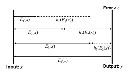
Figure 1: An illustration of the total work in a learning problem, visualized as the distance traveled from the input bar to the output bar. Different representations $E_{i}$ and different classifiers $h_{i}$ provide different effort.

Figure 1 illustrates the two sub-tasks and their roles in figuratively “transporting” an input $x$ towards a prediction with a probability of error below a small $\epsilon$. For the representation $E_{1}$, the best classifier $h_{1}$ falls short of this error requirement. The representation $E_{4}$ does not need an additional classifier because it is identical to the label. The representations $E_{2}$ and $E_{3}$ both admit classifiers $h_{2}$ and $h_{3}$ that meet the error threshold. Further, note, that $E_{3}$ leaves less work for the classifier than $E_{2}$, suggesting that it is a better representation as far as this task is concerned.

This illustration gives us the guiding principle for this work:

The quality of a representation $E$ for a task is a function of both the performance and the complexity of the best classifier $h$ over that representation.

Two observations follow from the above discussion. First, we cannot enumerate every possible classifier to find the best one. Other recent work, such as that of Xia et al. (2020) make a similar point. Instead, we need to resort to an approximation to evaluate representations. Second, trivially, the best representation for a task is identical to an accurate classifier; in the illustration in Figure 1, this is represented by $E_{4}$. However, such a representation is over-specialized to one task. In contrast, learned representations like BERT promise task-independent representations that support accurate classifiers.

2.2 $\epsilon$-Version Spaces

Given a classification task, we seek to disentangle the evaluation of a representation $E$ from the classifiers $h$ that are trained over it. To do so, the first step is to characterize all classifiers supported by a representation.

Classifiers are trained to find a hypothesis (i.e., a classifier) that is consistent with a training set. A representation $E$ admits a set of such hypotheses, and a learner chooses one of them. Consider the top-left example of Figure 2. There are many classifiers that separate the two classes; the figure shows two linear ($h_{1}$ and $h_{2}$) and one non-linear ($h_{3}$) example. Given a set $\mathcal{H}$ of classifiers of interest, the subset of classifiers that are consistent with a given dataset represents the version space with respect to $\mathcal{H}$ Mitchell (1982). To account for errors or noise in data, we define an $\epsilon$-version space: the set of hypothesis that can achieve less than $\epsilon$ error on a given dataset.

Let us formalize this definition. Suppose $\mathcal{H}$ represents the whole hypothesis space consisting of all possible classifiers $h$ of interest. The $\epsilon$-version space $V_{\epsilon}(\mathcal{H},E,D)$ expressed by a representation $E$ for a labeled dataset $D$ is defined as:

$${V_{\epsilon}\left(\mathcal{H},E,D\right)\triangleq\left\{h\in\mathcal{H}\mid err(h,E,D)\leq\epsilon\right\}}$$ (1)

where $err$ represents training error.

Note that the $\epsilon$-version space $V_{\epsilon}(\mathcal{H},E,D)$ is only a set of functions and does not involve any learning. However, understanding a representation requires examining its $\epsilon$-version space—a larger one would allow for easier learning.

In previous work, the quality of a representation $E$ for a task represented by a dataset $D$ is measured via properties of a specific $h\in V_{\epsilon}(\mathcal{H},E,D)$, typically a linear probe. Commonly measured properties include generalization error Kim et al. (2019), minimum description length of labels  Voita and Titov (2020) and complexity Whitney et al. (2020). Instead, we seek to directly evaluate the $\epsilon$-version space of a representation for a task, without committing to a restricted set of probe classifiers.

3 Approximating an $\epsilon$-Version Space

Although the notion of an $\epsilon$-version space is well defined, finding it for a given representation and task is impossible because it involves enumerating all possible classifiers. In this section, we will describe a heuristic to approximate the $\epsilon$-version space. We call this approach as DirectProbe.

3.1 Piecewise Linear Approximation

Each classifier in $V_{\epsilon}(\mathcal{H},E,D)$ is a decision boundary in the representation space that separates examples with different labels (see Figure 2, left). The decisions of a classifier can be mimicked by a set of piecewise linear functions. Figure 2 (middle) shows two examples. At the top is the simple case with linearly separable points. At the bottom is a more complicated case with a circular separator. The set of the piecewise linear function that matches its decisions needs at least three lines.

Figure 2: Using the piecewise linear functions to mimic decision boundaries on two different cases. The solid lines on the left are the real decision boundaries for a binary classification problem. The dashed lines in the middle are the piecewise linear functions used to mimic these decision boundaries. The gray area is the region that a separator must cross. The connected points in the right represent the convex regions that the piecewise linear separators lead to.

The ideal piecewise linear separator partitions training points into groups, each of which contains points with exactly one label. These groups can be seen as defining convex regions in the embedding space (see Figure 2, left). Any classifier in $V_{\epsilon}(\mathcal{H},E,D)$ must cross the regions between the groups with different labels; these are the regions that separate labels from each other, as shown in the gray areas in Figure 2 (middle). Inspired by this, we posit that these regions between groups with different labels, and indeed the partitions themselves, offer insight into $V_{\epsilon}(\mathcal{H},E,D)$.

3.2 Partitioning Training Data

Although finding the set of all decision boundaries remain hard, finding the regions between convex groups that these piecewise linear functions splits the data into is less so. Grouping data points in this fashion is related to a well-studied problem, namely clustering, and several recent works have looked at clustering of contextualized representations Reimers et al. (2019); Aharoni and Goldberg (2020); Gupta et al. (2020). In this work, we have a new clustering problem with the following criteria: (i) All points in a group have the same label.We need to ensure we are mimicking the decision boundaries. (ii) There are no overlaps between the convex hulls of each group.If convex hulls of two groups do not overlap, there must exist a line that can separates them, as guaranteed by the hyperplane separation theorem. (iii) Minimize the number of total groups.Otherwise, a simple solution is that each data point becomes a group by itself.

Note that the criteria do not require all points of one label to be grouped together. For example, in Figure 2 (bottom right), points of the circle (i.e., $\circ$) class are in three subgroups.

To summarize what we have so far: we transformed the problem of finding the $\epsilon$-version space into a clustering problem with specific criteria. Next, let us see a heuristic for partitioning the training set into clusters based on these criteria.

3.3 A Heuristic for Clustering

To find clusters as described in Section 3.2, we define a simple bottom-up heuristic clustering strategy that forms the basis of DirectProbe (Algorithm 1). In the beginning, each example $x_{i}$ with label $y_{i}$ in a training set $D$ is a cluster $C_{i}$ by itself. In each iteration, we select the closest pair of clusters with the same label and merge them (lines 4, 5). If the convex hull of the new cluster does not overlap with all other clusters, we keep this new cluster (line 9). Otherwise, we flag this pair (line 7) and choose the next closest pair of clusters. We repeat these steps till no more clusters can be merged.

Algorithm 1 DirectProbe: Bottom-up Clustering

1:A dataset $D$ with labeled examples $(x_{i},y_{i})$.

2:A set of clusters of points $\mathcal{C}$.

3:Initialize $C_{i}$ as the cluster for each $(x_{i},y_{i})\in D$

4:$\mathcal{C}=\{C_{0},C_{1},\cdots\},B=\emptyset$

5:repeat

6:     Select the closest pair $(C_{i},C_{j})\in\mathcal{C}$ which have the same label and is not flagged in $B$.

7:     $S\leftarrow C_{i}\cup C_{j}$

8:     if convex hull of $S$ overlaps with other elements of $\mathcal{C}$ then

9:         $B\leftarrow B\cup\{(C_{i},C_{j})\}$

10:     else

11:         Update $\mathcal{C}$ by removing $C_{i},C_{j}$ and adding $S$

12:     end if

13:until no more pairs can be merged

14:return $\mathcal{C}$

We define the distance between clusters $C_{i}$ and $C_{j}$ as the Euclidean distance between their centroids. Although Algorithm 1 does not guarantee the minimization criterion in Section 3.2 since it is greedy heuristic, we will see in our experiments that, in practice, it works well.

Overlaps Between Convex Hulls

A key point of Algorithm 1 is checking if the convex hulls of two sets of points overlap (line 6). Suppose we have two sets $C=\{x_{1}^{C},\ldots,x_{n}^{C}\}$ and $C^{\prime}=\{x_{1}^{C^{\prime}},\ldots,x_{m}^{C^{\prime}}\}$. We can restate this as the problem of checking if there is some vector $w\in\Re^{n}$ and a number $b\in\Re$ such that:

$$\forall x_{i}^{C}\in C, ~{}\quad w^{\top}E(x_{i}^{C})+b\geq 1,$$ (2)

$$\forall x_{j}^{C^{\prime}}\in{C^{\prime}}, ~{}\quad w^{\top}E(x_{j}^{C^{\prime}})+b\leq-1.$$

where $E$ is the representation under investigation.

We can state this problem as a linear program that checks for feasibility of the system of inequalities. If the LP problem is feasible, there must exist a separator between the two sets of points, and they do not overlap. In our implementation, we use the Gurobi optimizer Gurobi Optimization (2020) to solve the linear programs.

3.4 Noise: Controlling $\epsilon$

Clusters with only a small number of points could be treated as noise. Geometrically, a point in the neighborhood of other points with different labels could be thought of as noise. Other clusters can not merge with it because of the no-overlap constraint. As a result, such clusters will have only a few points (one or two in practice). If we want zero error rate on the training data, we can keep these noise points; if we allow a small error rate $\epsilon$, then we can remove these noise clusters. In our experiments, for simplicity, we keep all clusters.

4 Representations, Tasks and Classifiers

Before looking at the analysis offered by the partitions obtained via DirectProbe in Section 5, let us first enumerate the English NLP tasks and representations we will encounter.

4.1 Representations

Our main experiments focus on BERT${}_{\text{base,cased}}$, and we also show additional analysis on other contextual representations: ELMo Peters et al. (2018), BERT${}_{\text{large,cased}}$ Devlin et al. (2019), RoBERTa${}_{\text{base}}$ and RoBERTa${}_{\text{large}}$ Liu et al. (2019b). We refer the reader to the Appendix C for further details about these embeddings.

We use the average of subword embeddings as the token vector for the representations that use subwords. We use the original implementation of ELMo, and the HuggingFace library Wolf et al. (2020) for the others.

4.2 Tasks

We conduct our experiments on five NLP tasks that cover the varied usages of word representations (token-based, span-based, and token pairs) and include both syntactic and semantic prediction problems. The Appendix D has more details about the tasks to help with replication.

Preposition supersense disambiguation represents a pair of tasks, involving classifying a preposition’s semantic role (SS-role) and semantic function (SS-func). Following the previous work Liu et al. (2019a), we only use the single-token prepositions in the Streusle v4.2 corpus Schneider et al. (2018).

Part-of-speech tagging (POS) is a token level prediction task. We use the English portion of the parallel universal dependencies treebank (ud-pud Nivre et al., 2016).

Semantic relation (SR) is the task of predicting the semantic relation between pairs of nominals. We use the dataset of semeval2010 task 8 Hendrickx et al. (2010). To represent the pair of nominals, we concatenate their embeddings. Some nominals could be spans instead of individual tokens, and we represent them via the average embedding of the tokens in the span.

Dependency relation (DEP) is the task of predicting the syntactic dependency relation between a token $w_{head}$ and its modifier $w_{mod}$. We use the universal dependency annotation of the English web treebank Bies et al. (2012). As with semantic relations, to represent the pair of tokens, we concatenate their embeddings.

4.3 Classifier Accuracy

The key starting point of this work is that restricting ourselves to linear probes may be insufficient. To validate the results of our analysis, we evaluate a large collection of classifiers—from simple linear classifiers to two-layers neural networks—for each task. For each one, we choose the best hyper-parameters using cross-validation. From these classifiers, we find the best test accuracy of each task and representation. All classifiers are trained with the scikit-learn library Pedregosa et al. (2011). To reduce the impact of randomness, we trained each classifier $10$ times with different initializations, and report their average accuracy. The Appendix E summarizes the best classifiers we found and their performance.

5 Experiments and Analysis

DirectProbe helps partition an embedding space for a task, and thus characterize its $\epsilon$-version space. Here, we will see that these clusters do indeed characterize various linguistic properties of the representations we consider.

5.1 Number of Clusters

The number of clusters is an indicator of the linear separability of representations for a task.

The best scenario is when the number of clusters equals the number of labels. In this case, examples with the same label are placed close enough by the representation to form a cluster that is separable from other clusters. A simple linear multi-class classifier can fit well in this scenario. In contrast, if the number of clusters is more than the number of labels, then some labels are distributed across multiple clusters (as in Figure 2, bottom). There must be a non-linear decision boundary. Consequently, this scenario calls for a more complex classifier, e.g., a multi-layer neural network.

In other words, using the clusters, and without training a classifier, we can answer the question: can a linear classifier fit the training set for a task with a given representation?

To validate our predictions, we use the training accuracy of a linear SVM Chang and Lin (2011) classifier. If a linear SVM can perfectly fit ($100\%$ accuracy) a training set, then there exist linear decision boundaries that separate the labels. Table 1 shows the linearity experiments on the POS task, which has 17 labels in total. All representations except RoBERTa${}_{\text{large}}$ have $17$ clusters, suggesting a linearly separable space, which is confirmed by the SVM accuracy. We conjecture that this may be the reason why linear models usually work for BERT-family models. Of course, linear separability does not mean the task is easy or that the best classifier is a linear one. We found that, while most representations we considered are linearly separable for most of our tasks, the best classifier is not always linear. We refer the reader to Appendix E for the full results.

Embedding	Linear SVM	#Clusters
	Training Accuracy
BERT${}_{\text{base,cased}}$	100	17
BERT${}_{\text{large,cased}}$	100	17
RoBERTa${}_{\text{base}}$	100	17
RoBERTa${}_{\text{large}}$	99.97	1487
ELMo	100	17

Table 1: Linearity experiments on POS tagging task. Our POS tagging task has $17$ labels in total. Both linear SVM and the number of clusters suggest that RoBERTa${}_{\text{large}}$ is non-linear while others are all linear, which means the best classifier for RoBERTa${}_{\text{large}}$ is not a linear model. More details can be found in Appendix E.

5.2 Distances between Clusters

As we mentioned in Section 3.1, a learning process seeks to find a decision boundary that separates clusters with different labels. Intuitively, a larger gap between them would make it easier for a learner to find a suitable hypothesis $h$ that generalizes better.

We use the distance between convex hulls of clusters as an indicator of the size of these gaps. We note that the problem of computing the distance between convex hulls of clusters is equivalent to finding the maximum margin separator between them. To find the distance between two clusters, we train a linear SVM Chang and Lin (2011) that separates them and compute its margin. The distance we seek is twice the margin. For a given representation, we are interested in the minimum distance across all pairs of clusters with different labels.

5.2.1 Minimum Distance of Different Layers

Higher layers usually have larger $\epsilon$-version spaces.

Different layers of BERT play different roles when encoding liguistic information Tenney et al. (2019). To investigate the geometry of different layers of BERT, we apply DirectProbe to each layer of BERT${}_{\text{base,cased}}$ for all five tasks. Then, we computed the minimum distances among all pairs of clusters with different labels. By comparing the minimum distances of different layers, we answer the question: how do different layers of BERT differ in their representations for a task?

Figure 3 shows the results on all tasks. In each subplot, the horizontal axis is the layer index. For each layer, the blue circles (left vertical axis) is the best classifier accuracy, and the red triangles (right vertical axis) is the minimum distance described above. We observe that both best classifier accuracy and minimum distance show similar trends across different layers: first increasing, then decreasing. It shows that minimum distance correlates with the best performance for an embedding space, though it is not a simple linear relation. Another interesting observation is the decreasing performance and minimum distance of higher layers, which is also corroborated by Ethayarajh (2019) and Liu et al. (2019a).

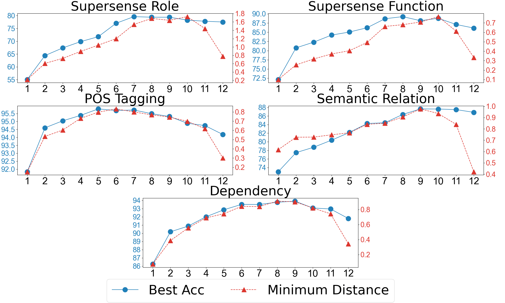
Figure 3: Here we juxtapose the minimum distances between clusters and the best classifier accuracy for all 12 layers. The horizontal axis is the layer index of BERT${}_{\text{base,cased}}$; the left vertical axis is the best classifier accuracy and the right vertical axis is the minimum distance between all pairs of clusters.

5.2.2 Impact of Fine-tuning

Fine-tuning expands the $\epsilon$-version space.

Past work Peters et al. (2019); Arase and Tsujii (2019); Merchant et al. (2020) has shown that fine-tuning pre-trained models on a specific task improves performance, and fine-tuning is now the de facto procedure for using contextualized embeddings. In this experiment, we try to understand why fine-tuning can improve performance. Without training classifiers, we answer the question: What changes in the embedding space after fine-tuning?

We conduct the experiments described in Section 5.2.1 on the last layer of BERT${}_{\text{base,cased}}$ before and after fine-tuning for all tasks. Table 2 shows the results. We see that after fine-tuning, both the best classifier accuracy and minimum distance show a big boost. It means that fine-tuning pushes the clusters away from each other in the representation space, which results in a larger $\epsilon$-version space. As we discussed in Section 5.2, a larger $\epsilon$-version space admits more good classifiers and allows for better generalization.

Task		Min Distance	Best Acc
SS-role	original	0.778	77.51
	fine-tuned	4.231	81.62
SS-func	original	0.333	86.13
	fine-tuned	2.686	88.4
POS	original	0.301	93.59
	fine-tuned	0.7696	95.95
SR	original	0.421	86.85
	fine-tuned	4.734	90.03
DEP	original	0.345	91.52
	fine-tuned	1.075	94.82

Table 2: The best performance and the minimum distances between all pairs of clusters of the last layer of BERT${}_{\text{base,cased}}$ before and after fine-tuning.

5.2.3 Label Confusion

Small distances between clusters can confuse a classifier.

By comparing the distances between clusters, we can answer the question: Which labels for a task are more confusable?

We compute the distances between all the pairs of labels based on the last layer of BERT${}_{\text{base,cased}}$. Based on an even split of the distances, we partition all label pairs into three bins: small, medium, and large. For each task, we use the predictions of the best classifier to compute the number of misclassified label pairs for each bin. For example, if the clusters associated with the part of speech tags ADV and ADJ are close to each other, and the best classifier misclassified ADV as ADJ, we put this error pair into the bin of small distance. The distribution of all errors is shown in Table 3. This table shows that a large majority of the misclassified labels are concentrated in the small distance bin. For example, in the supersense role task (SS-role), $97.17\%$ of the errors happened in small distance bin. The number of label pairs of each bin is shown in the parentheses. Table 3 shows that small distances between clusters indeed confuse a classifier and we can detect it without training classifiers.

Task	Small	Medium	Large
	Distance	Distance	Distance
SS-role	97.17% (555)	2.83% (392)	0% (88)
SS-func	96.88% (324)	3.12% (401)	0% (55)
POS	99.19% (102)	0.81% (18)	0% (16)
SR	93.20% (20)	6.80% (20)	0% (5)
DEP	99.97% (928)	0.03% (103)	0% (50)

Table 3: Error distribution based on different distance bins. The number of label pairs in each bin is shown in the parentheses.

5.3 By-product: A Parameter-free Classifier

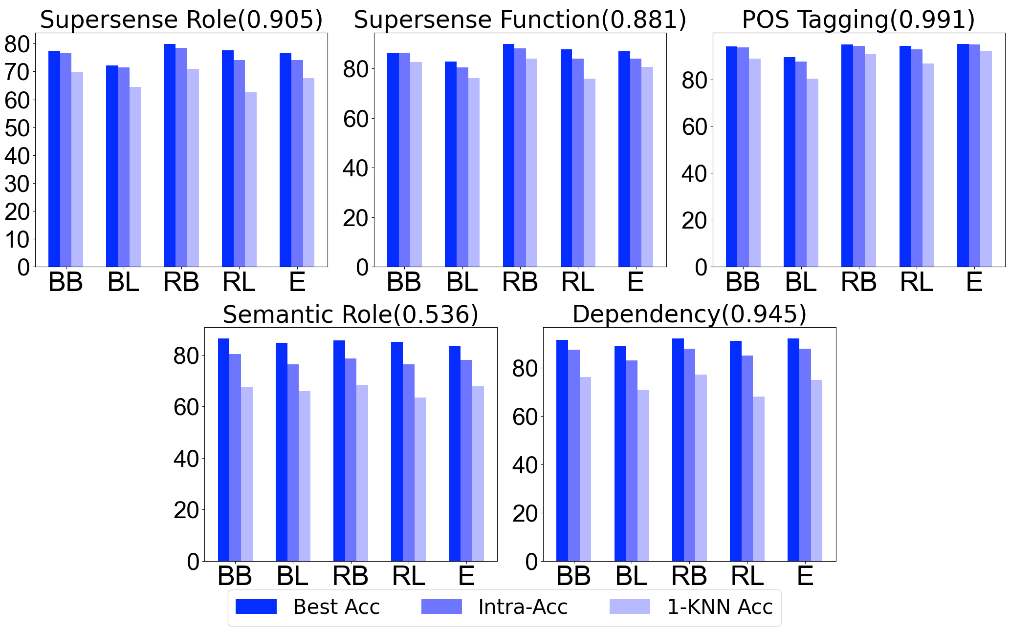
Figure 4: Comparison between the best classifier accuracy, intra-accuracy, and 1-kNN accuracy. The X-axis is different representation models. BB: BERT${}_{\text{base,cased}}$, BL: BERT${}_{\text{large,cased}}$, RB: RoBERTa${}_{\text{base}}$, RL: RoBERTa${}_{\text{large}}$, E: ELMo. The pearson correlation coefficient between best classifier accuracy and intra-accuracy is shown in the parentheses alongside each task title. This figure is best viewed in color.

We can predict the expected performance of the best classifier.

Any $h\in V_{\epsilon}(\mathcal{H},E,D)$ is a predictor for the task $D$ on the representation $E$. As a by-product of the clusters from DirectProbe, we can define a predictor. The prediction strategy is simple: for a test example, we assign it to its closest cluster. Indeed, if the label of the cluster is the true label of the test point, then we know that there exists some classifier that allows this example to be correctly labeled. We can verify the label every test point and compute the aggregate accuracy to serve as an indicator of the generalization ability of the representation at hand. We call this accuracy the intra-accuracy. In other words, without training classifiers, we can answer the question: given a representation, what is the expected performance of the best classifier for a task?

Figure 4 compares the best classifier accuracy, and the intra-accuracy of the last layer of different embeddings. Because our assignment strategy is similar to nearest neighbor classification (1-kNN), which assigns the unlabelled test point to its closest labeled point, the figure also compares to the 1-kNN accuracy.

First, we observe that intra-accuracy always outperforms the simple 1-kNN classifier, showing that DirectProbe can use more information from the representation space. Second, we see that the intra-accuracy is close to the best accuracy for some tasks (Supersense tasks and POS tagging). Moreover, all the pearson correlation coefficients between best accuracy and intra-accuracy (showed in the parentheses alongside each task title) suggest a high linear correlation between best classifier accuracy and intra-accuracy. That is, the intra-accuracy can be a good predictor of the best classifier accuracy for a representation. From this, we argue that intra-accuracy can be interpreted as a benchmark accuracy of a given representation without actually training classifiers.

5.4 Case Study: Identifying Difficult Examples

The distances between a test point and all the clusters from the training set can not only be used to predict the label but also can be used to identify difficult examples as per a given representation. Doing so could lead to re-annotation of the data, and perhaps lead to cleaner data, or to improved embeddings. Using the supersense role task, we show a randomly chosen example of a mismatch between the annotated label and the BERT${}_{\text{base,cased}}$ neighborhood:

…our new mobile number is …

The data labels the word our as Gestalt, while the embedding places it in the neighborhood of Possessor. The annotation guidelines for these labels Schneider et al. (2017) notes that Gestalt is a supercategory of Possessor. The latter is specifically used to identify cases where the possessed item is alienable and has monetary value. From this definition, we see that though the annotated label is Gestalt, it could arguably also be a Possessor if phone numbers are construed as alienable possessions that have monetary value. Importantly, it is unclear whether BERT${}_{\text{base,cased}}$ makes this distinction. Other examples we examined required similarly nuanced analysis. This example shows DirectProbe can be used to identify examples in datasets that are potentially mislabeled, or at least, require further discussion.

6 Related Work and Discussion

In addition to the classifier based probes described in the rest of the paper, a complementary line of work focuses on probing the representations using a behavior-based methodology. Controlled test sets Şenel et al. (2018); Jastrzebski et al. (2017) are designed and errors are analyzed to reverse-engineer what information can be encoded by the model (e.g., Marvin and Linzen, 2018; Ravichander et al., 2020; Wu et al., 2020). Another line of work probes the space by “opening up” the representation space or the model (e.g., Michel et al., 2019; Voita et al., 2019). There are some efforts to inspect the space from a geometric perspective (e.g., Ethayarajh, 2019; Mimno and Thompson, 2017). Our work extends this line of work to connect the geometric structure of embedding space with classifier performance without actually training a classifier.

Recent work Pimentel et al. (2020b); Voita and Titov (2020); Zhu and Rudzicz (2020) probe representations from an information theoretic perspective. These efforts still need a probability distribution $p(y|x)$ from a trained classifier. In Section 5.3, we use clusters to predict labels. In the same vein, the conditional probability $p(y|x)$ can be obtained by treating the negative distances between the test point $x$ and all clusters as predicted scores and normalizing via softmax. Our formalization can fit into the information theoretic analysis and yet avoid training a classifier.

Our analysis and experiments open new directions for further research:

Novel pre-training target: The analysis presented here informs us that larger distance between clusters can improve classifiers. This could guide loss function design when pre-training representations.

Quality of a representation: In this paper, we focus on the accuracy of a representation. We could seek to measure other properties (e.g., complexity) or proxies for them. These analytical approaches can be applied to the $\epsilon$-version space to further analyze the quality of the representation space.

Theory of representation: Learning theory, e.g. VC-theory Vapnik (2013), describes the learnability of classifiers; representation learning lacks of such theoretical analysis. The ideas explored in this work ($\epsilon$-version spaces, distances between clusters being critical) could serve as a foundation for an analogous theory of representations.

7 Conclusion

In this work, we ask the question: what makes a representation good for a task? We answer it by developing DirectProbe, a heuristic approach builds upon hierarchical clustering to approximate the $\epsilon$-version space. Via experiments with several contextualized embeddings and linguistic tasks, we showed that DirectProbe can help us understand the geometry of the embedding space and ascertain when a representation can successfully be employed for a task.

Acknowledgments

We thank the members of the Utah NLP group and Nathan Schneider for discussions and valuable insights, and reviewers for their helpful feedback. We also thank the support of NSF grants #1801446 (SATC) and #1822877 (Cyberlearning).

Appendix A DirectProbe in Practice

In practice, we apply several techniques to speed up the probing process. Firstly, we add two caching strategies:

Black List

Suppose we know two clusters $A$ and $B$ can not be merged, then $A^{\prime}$ and $B^{\prime}$ cannot be merged either if $A\subseteq A^{\prime}$ and $B\subseteq B^{\prime}$

White List

Suppose we know two clusters $A$ and $B$ can be merged, then $A^{\prime}$ and $B^{\prime}$ can be merged too if $A^{\prime}\subseteq A$ and $B^{\prime}\subseteq B$

These two observations allow us to cache previous decisions in checking whether two clusters overlap. Applying these caching strategies can help us avoid unnecessary checking for overlap, which is time-consuming.

Secondly, instead of merging from the start to the end and checking at every step, we directly keep merging to the end without any overlap checking. After we arrived at the end, we start checking backwards to see if there is an overlap. If final clusters have overlaps, we find the step of the first error, correct it and keep merging. Merging to the end can also help us avoid plenty of unnecessary checking because, in most representations, the first error usually happens only in the final few merges. Algorithm 2 shows the whole algorithm.

Algorithm 2 DirectProbe in Practice

1:A dataset $D$ with labeled examples $(x_{i},y_{i})$.

2:A set of clusters of points $\mathcal{C}$.

3:Initialize $C_{i}$ as the cluster for each $(x_{i},y_{i})\in D$

4:$\mathcal{C}=\{C_{0},C_{1},\cdots\}$

5:Keep merging the closest pairs who have the same label in $\mathcal{C}$ without overlapping checking.

6:if There are overlappings in $\mathcal{C}$ then

7:     Find the step $k$ that first overlap happens.

8:     Rebuild $\mathcal{C}$ from step $k-1$

9:     Keeping merging the closest pairs who have the same label in $\mathcal{C}$ with overlapping checking.

10:end if

11:return $\mathcal{C}$

Table 4 shows the runtime comparison between DirectProbe and training classifiers.

	DirectProbe		Classifier
	Clustering	Predict	CV	Train-Test
SS-role	1 min	7 min	1.5 hours	1 hour
SS-func	1.5 min	5.5 min	1 hour	1 hour
POS	14 min	43 min	3.5 hours	2 hours
SR	10 min	22 min	50 min	1 hour
DEP	3 hours	3 hours	20 hours	11 hours

Table 4: The comparison of running time between DirectProbe and training classifiers using the setting described in Appendix B. The time is computed on the BERT${}_{\text{base,cased}}$ space. DirectProbe and classifiers run on the same machine.

Appendix B Classifier Training Details

We train $3$ different kinds of classifiers in order to find the best one: Logistic Regression, a one-layer neural network with hidden layer size of $(32,64,128,256)$ and two-layers neural network with hidden layer sizes of $(32,64,128,256)\times(32,64,128,256)$. All neural networks use ReLU as the activation function and optimized by Adam Kingma and Ba (2015). The cross-validation process chooses the weight of each regularizer of each classifier. The weight range is from $10^{-7}$ to $10^{0}$. We set the maximum iterations to be $1000$. After choosing the best hyperparameters, each specific classifier is trained $10$ times with different initializations.

Appendix C Summary of Representations

Table 5 summarizes all the representations in our experiments.

Representations	#Parameters	Dimensions
BERT${}_{\text{base,cased}}$	110M	768
BERT${}_{\text{large,cased}}$	340M	1024
RoBERTa${}_{\text{base}}$	125M	768
RoBERTa${}_{\text{large}}$	355M	1024
ELMo	93.6M	1024

Table 5: Statistics of the five representations in our experiments.

Appendix D Summary of Tasks

In this work, we conduct experiments on $5$ tasks, which is designed to cover different usages of representations. Table 6 summarizes these tasks.

Task	#Training	#Test	Token-based	Span-based	Pair-wise	Semantic	Syntax
Supersense-role	4282	457	$\surd$			$\surd$
Supersense-function	4282	457	$\surd$			$\surd$
POS	16860	4323	$\surd$				$\surd$
Dependency Relation	42081	4846			$\surd$		$\surd$
Semantic Relation	8000	2717		$\surd$	$\surd$	$\surd$

Table 6: Statistics of the five tasks with their different characteristics.

Appendix E Classifier Results v.s. DirectProbe Results

Table 8 summarizes the results of the best classifier for each representation and task. The meanings of each column are as follows:

• Embedding: The name of representation.

• Best classification: The accuracy of the best classifier among $21$ different classifiers. Each classifier run $10$ times with different starting points. The final accuracy is the average accuracy of these $10$ runs.

• Intra-accuracy: The prediction accuracy by assigning test examples to their closest clusters.

• Type: The type of the best classifier. e.g. $(256,)$ means one-layer neural network with hidden size $256$ and $(256,128)$ means two-layer neural network with hidden sizes $256$ and $128$ respectively.

• Parameters: The number of parameters of the best classifier.

• Linear SVM: Training accuracy of a linear SVM classifier.

• #Clusters: The number of final clusters after probing.

Appendix F Detailed Classification Results

Table 7 shows the detailed classification results on Supersense-role task using the same settings described in Appendix B. In this table, we record the difference between the minimum and maximum test accuracy of the $10$ runs of each classifier. The maximum difference for each representation is highlighted by the underlines. The best performance of each representation is highlighted by the bold numbers. From this table, we observe: (i) the difference between different runs of the same classifier can be as large as 4-7%, which can not be ignored; (ii) different representation requires different model architecture to achieve its best performance.

Model	Specific	BERT${}_{\text{base,cased}}$			BERT${}_{\text{large,cased}}$			RoBERTa${}_{\text{base}}$			RoBERTa${}_{\text{large}}$			ELMo
Family	Model	Min	Max	Diff	Min	Max	Diff	Min	Max	Diff	Min	Max	Diff	Min	Max	Diff
Linear	LR	75.93	76.59	0.66	72.21	72.43	0.22	79.65	80.09	0.44	77.46	77.90	0.44	76.37	77.02	0.65
One-layer	(32,)	75.27	78.56	3.29	70.24	73.09	2.85	77.9	79.87	1.97	74.84	78.34	3.5	74.4	75.93	1.53
	(64,)	76.37	78.56	2.19	71.33	72.87	1.54	78.56	80.74	2.18	76.59	77.68	1.09	73.74	75.93	2.19
	(128,)	75.71	77.9	2.19	70.46	73.3	2.84	77.9	80.53	2.63	75.71	77.46	1.75	73.52	76.15	2.63
	(256,)	75.27	78.12	2.85	70.68	73.96	3.28	78.34	80.96	2.62	74.84	77.9	3.06	73.96	76.81	2.85
Two-layers	(32,32)	71.99	76.81	4.82	67.4	70.68	3.28	75.71	79.43	3.72	70.68	74.62	3.94	70.24	73.96	3.72
	(32,64)	73.3	75.49	2.19	68.49	73.3	4.81	76.15	78.99	2.84	72.21	76.37	4.16	71.33	76.81	5.48
	(32,128)	73.74	75.27	1.53	67.61	72.65	5.04	76.15	80.09	3.94	72.65	76.81	4.16	70.02	74.4	4.38
	(32,256)	73.52	76.15	2.63	67.18	70.68	3.5	74.18	77.46	3.28	71.77	74.84	3.07	72.43	74.62	2.19
	(64,32)	73.52	76.59	3.07	67.61	72.87	5.26	75.93	78.56	2.63	71.33	75.93	4.6	71.99	75.49	3.5
	(64,64)	72.87	76.59	3.72	68.05	71.77	3.72	76.81	79.21	2.4	73.74	75.49	1.75	73.52	75.49	1.97
	(64,128)	73.09	76.81	3.72	69.37	72.43	3.06	76.81	79.21	2.4	72.65	75.49	2.84	72.87	75.27	2.4
	(64,256)	73.96	76.59	2.63	68.49	71.55	3.06	76.59	78.77	2.18	73.52	76.37	2.85	73.3	76.59	3.29
	(128,32)	72.65	77.24	4.59	70.02	72.43	2.41	76.59	80.53	3.94	73.74	75.93	2.19	72.43	75.93	3.5
	(128,64)	73.74	77.02	3.28	68.93	73.3	4.37	76.59	79.87	3.28	72.65	75.93	3.28	72.21	76.37	4.16
	(128,128)	74.84	77.24	2.4	69.37	72.43	3.06	77.46	79.21	1.75	72.87	75.71	2.84	73.52	76.15	2.63
	(128,256)	73.74	77.24	3.5	64.33	72.21	7.88	77.02	80.74	3.72	72.87	76.15	3.28	73.09	76.59	3.5
	(256,32)	73.74	78.12	4.38	68.05	73.3	5.25	77.68	80.31	2.63	73.74	75.93	2.19	72.87	75.71	2.84
	(256,64)	75.49	78.77	3.28	68.93	72.43	3.5	77.68	80.09	2.41	73.74	75.71	1.97	72.87	76.15	3.28
	(256,128)	75.27	78.77	3.5	70.46	73.96	3.5	77.9	80.74	2.84	73.74	77.02	3.28	73.96	76.37	2.41
	(256,256)	75.71	78.34	2.63	66.74	73.52	6.78	78.12	81.18	3.06	74.84	76.37	1.53	73.3	75.71	2.41

Table 7: Classification results on Supersense role task. Each specific classifier is trained ten times with different initializations. We record the minimum and maximum performance of these ten runs. Diff is the difference between the minimum and maximum performance. Bold number highlights the best performance of each representation. Underlines highlights the maximum difference between ten runs. See Appendix F for a discussion.

Task	Embedding	Best classification	Intra-accuracy	Type	Parameters	Linear SVM	#cluster
SS-role	BERT${}_{\text{base,cased}}$	$77.48\pm 0.92$	76.58	(256,128)	235264	100	46
	BERT${}_{\text{large,cased}}$	$72.25\pm 0.09$	71.55	linear	47104	100	46
	RoBERTa${}_{\text{base}}$	$79.85\pm 0.15$	78.56	linear	35328	100	46
	RoBERTa${}_{\text{large}}$	$77.7\pm 0.18$	74.18	linear	47104	100	46
	ELMo	$76.7\pm 0.24$	74.18	linear	47104	100	46
SS-func	BERT${}_{\text{base,cased}}$	$86.3\pm 0.44$	86.21	(128,)	103424	100	40
	BERT${}_{\text{large,cased}}$	$82.84\pm 0.73$	80.53	(256,)	272384	100	40
	RoBERTa${}_{\text{base}}$	$89.87\pm 0.51$	88.18	(256,)	206848	100	40
	RoBERTa${}_{\text{large}}$	$87.72\pm 0.56$	84.03	(256,128)	300032	100	40
	ELMo	$86.87\pm 0.31$	84.03	linear	40960	100	40
POS	BERT${}_{\text{base,cased}}$	$94.11\pm 0.14$	93.59	(256,256)	266496	100	17
	BERT${}_{\text{large,cased}}$	$89.54\pm 0.34$	87.69	(128,256)	168192	100	17
	RoBERTa${}_{\text{base}}$	$95\pm 0.09$	94.26	(128,256)	135424	100	17
	RoBERTa${}_{\text{large}}$	$94.25\pm 0.19$	92.92	(128,)	133248	99.97	1487
	ELMo	$95.08\pm 0.1$	94.93	(256,)	266496	100	17
Semantic Relation	BERT${}_{\text{base,cased}}$	$86.43\pm 0.28$	80.27	(256,)	395776	100	10
	BERT${}_{\text{large,cased}}$	$84.71\pm 0.27$	76.41	(128,256)	297472	100	10
	RoBERTa${}_{\text{base}}$	$85.55\pm 0.28$	78.58	(256,32)	401728	100	10
	RoBERTa${}_{\text{large}}$	$85.04\pm 0.23$	76.26	(256,)	526848	100	10
	ELMo	$83.47\pm 0.28$	78.06	(128,128)	279808	100	10
Dependency	BERT${}_{\text{base,cased}}$	$91.52\pm 0.25$	87.49	(256,)	405248	100	47
	BERT${}_{\text{large,cased}}$	$88.9\pm 0.38$	83.06	(256,)	536320	100	47
	RoBERTa${}_{\text{base}}$	$92.24\pm 0.03$	87.99	linear	72192	100	47
	RoBERTa${}_{\text{large}}$	$91.18\pm 0.04$	85.06	linear	96256	100	47
	ELMo	$92.21\pm 0.25$	88.05	(256,)	536320	100	47

Table 8: Intra-accuracy results on $5$ tasks, compared against the best classifier results. See Appendix E for details about each column.

References

- Aharoni and Goldberg (2020) Roee Aharoni and Yoav Goldberg. 2020. Unsupervised domain clusters in pretrained language models. In Proceedings of the 58th Annual Meeting of the Association for Computational Linguistics, pages 7747–7763, Online. Association for Computational Linguistics.
- Alain and Bengio (2017) Guillaume Alain and Yoshua Bengio. 2017. Understanding intermediate layers using linear classifier probes. In International Conference on Learning Representations.
- Arase and Tsujii (2019) Yuki Arase and Jun’ichi Tsujii. 2019. Transfer fine-tuning: A BERT case study. In Proceedings of the 2019 Conference on Empirical Methods in Natural Language Processing and the 9th International Joint Conference on Natural Language Processing (EMNLP-IJCNLP), pages 5393–5404, Hong Kong, China. Association for Computational Linguistics.
- Bengio et al. (2013) Y Bengio, A Courville, and P Vincent. 2013. Representation learning: a review and new perspectives. IEEE transactions on pattern analysis and machine intelligence, 35(8):1798.
- Bies et al. (2012) Ann Bies, Justin Mott, Colin Warner, and Seth Kulick. 2012. English web treebank. Linguistic Data Consortium, Philadelphia, PA.
- Chang and Lin (2011) Chih-Chung Chang and Chih-Jen Lin. 2011. Libsvm: A library for support vector machines. ACM transactions on intelligent systems and technology (TIST), 2(3):1–27.
- Conneau et al. (2018) Alexis Conneau, German Kruszewski, Guillaume Lample, Loïc Barrault, and Marco Baroni. 2018. What you can cram into a single $&!#* vector: Probing sentence embeddings for linguistic properties. In Proceedings of the 56th Annual Meeting of the Association for Computational Linguistics (Volume 1: Long Papers), pages 2126–2136, Melbourne, Australia. Association for Computational Linguistics.
- Devlin et al. (2019) Jacob Devlin, Ming-Wei Chang, Kenton Lee, and Kristina Toutanova. 2019. BERT: Pre-training of deep bidirectional transformers for language understanding. In Proceedings of the 2019 Conference of the North American Chapter of the Association for Computational Linguistics: Human Language Technologies, Volume 1 (Long and Short Papers), pages 4171–4186, Minneapolis, Minnesota. Association for Computational Linguistics.
- Eger et al. (2019) Steffen Eger, Andreas Rücklé, and Iryna Gurevych. 2019. Pitfalls in the evaluation of sentence embeddings. In Proceedings of the 4th Workshop on Representation Learning for NLP (RepL4NLP-2019), pages 55–60, Florence, Italy. Association for Computational Linguistics.
- Ethayarajh (2019) Kawin Ethayarajh. 2019. How contextual are contextualized word representations? comparing the geometry of BERT, ELMo, and GPT-2 embeddings. In Proceedings of the 2019 Conference on Empirical Methods in Natural Language Processing and the 9th International Joint Conference on Natural Language Processing (EMNLP-IJCNLP), pages 55–65, Hong Kong, China. Association for Computational Linguistics.
- Goodwin et al. (2020) Emily Goodwin, Koustuv Sinha, and Timothy J. O’Donnell. 2020. Probing linguistic systematicity. In Proceedings of the 58th Annual Meeting of the Association for Computational Linguistics, pages 1958–1969, Online. Association for Computational Linguistics.
- Gupta et al. (2020) Vikram Gupta, Haoyue Shi, Kevin Gimpel, and Mrinmaya Sachan. 2020. Clustering contextualized representations of text for unsupervised syntax induction. arXiv preprint arXiv:2010.12784.
- Gurobi Optimization (2020) LLC Gurobi Optimization. 2020. Gurobi optimizer reference manual.
- Hendrickx et al. (2010) Iris Hendrickx, Su Nam Kim, Zornitsa Kozareva, Preslav Nakov, Diarmuid Ó Séaghdha, Sebastian Padó, Marco Pennacchiotti, Lorenza Romano, and Stan Szpakowicz. 2010. SemEval-2010 task 8: Multi-way classification of semantic relations between pairs of nominals. In Proceedings of the 5th International Workshop on Semantic Evaluation, pages 33–38, Uppsala, Sweden. Association for Computational Linguistics.
- Hewitt and Liang (2019) John Hewitt and Percy Liang. 2019. Designing and interpreting probes with control tasks. In Proceedings of the 2019 Conference on Empirical Methods in Natural Language Processing and the 9th International Joint Conference on Natural Language Processing (EMNLP-IJCNLP), pages 2733–2743, Hong Kong, China. Association for Computational Linguistics.
- Jastrzebski et al. (2017) Stanisław Jastrzebski, Damian Leśniak, and Wojciech Marian Czarnecki. 2017. How to evaluate word embeddings? on importance of data efficiency and simple supervised tasks. arXiv preprint arXiv:1702.02170.
- Jawahar et al. (2019) Ganesh Jawahar, Benoît Sagot, and Djamé Seddah. 2019. What does BERT learn about the structure of language? In Proceedings of the 57th Annual Meeting of the Association for Computational Linguistics, pages 3651–3657, Florence, Italy. Association for Computational Linguistics.
- Kassner and Schütze (2020) Nora Kassner and Hinrich Schütze. 2020. Negated and misprimed probes for pretrained language models: Birds can talk, but cannot fly. In Proceedings of the 58th Annual Meeting of the Association for Computational Linguistics, pages 7811–7818, Online. Association for Computational Linguistics.
- Kim et al. (2019) Najoung Kim, Roma Patel, Adam Poliak, Patrick Xia, Alex Wang, Tom McCoy, Ian Tenney, Alexis Ross, Tal Linzen, Benjamin Van Durme, Samuel R. Bowman, and Ellie Pavlick. 2019. Probing what different NLP tasks teach machines about function word comprehension. In Proceedings of the Eighth Joint Conference on Lexical and Computational Semantics (*SEM 2019), pages 235–249, Minneapolis, Minnesota. Association for Computational Linguistics.
- Kingma and Ba (2015) Diederik P. Kingma and Jimmy Ba. 2015. Adam: A Method for Stochastic Optimization. In 3rd International Conference on Learning Representations, ICLR 2015, San Diego, CA, USA, May 7-9, 2015, Conference Track Proceedings.
- Kovaleva et al. (2019) Olga Kovaleva, Alexey Romanov, Anna Rogers, and Anna Rumshisky. 2019. Revealing the dark secrets of BERT. In Proceedings of the 2019 Conference on Empirical Methods in Natural Language Processing and the 9th International Joint Conference on Natural Language Processing (EMNLP-IJCNLP), pages 4365–4374, Hong Kong, China. Association for Computational Linguistics.
- Krasnowska-Kieraś and Wróblewska (2019) Katarzyna Krasnowska-Kieraś and Alina Wróblewska. 2019. Empirical linguistic study of sentence embeddings. In Proceedings of the 57th Annual Meeting of the Association for Computational Linguistics, pages 5729–5739, Florence, Italy. Association for Computational Linguistics.
- Kulmizev et al. (2020) Artur Kulmizev, Vinit Ravishankar, Mostafa Abdou, and Joakim Nivre. 2020. Do neural language models show preferences for syntactic formalisms? In Proceedings of the 58th Annual Meeting of the Association for Computational Linguistics, pages 4077–4091, Online. Association for Computational Linguistics.
- Liu et al. (2019a) Nelson F. Liu, Matt Gardner, Yonatan Belinkov, Matthew E. Peters, and Noah A. Smith. 2019a. Linguistic knowledge and transferability of contextual representations. In Proceedings of the 2019 Conference of the North American Chapter of the Association for Computational Linguistics: Human Language Technologies, Volume 1 (Long and Short Papers), pages 1073–1094, Minneapolis, Minnesota. Association for Computational Linguistics.
- Liu et al. (2019b) Yinhan Liu, Myle Ott, Naman Goyal, Jingfei Du, Mandar Joshi, Danqi Chen, Omer Levy, Mike Lewis, Luke Zettlemoyer, and Veselin Stoyanov. 2019b. Roberta: A robustly optimized bert pretraining approach. arXiv preprint arXiv:1907.11692.
- Marvin and Linzen (2018) Rebecca Marvin and Tal Linzen. 2018. Targeted syntactic evaluation of language models. In Proceedings of the 2018 Conference on Empirical Methods in Natural Language Processing, pages 1192–1202, Brussels, Belgium. Association for Computational Linguistics.
- Merchant et al. (2020) Amil Merchant, Elahe Rahimtoroghi, Ellie Pavlick, and Ian Tenney. 2020. What happens to BERT embeddings during fine-tuning? In Proceedings of the Third BlackboxNLP Workshop on Analyzing and Interpreting Neural Networks for NLP, pages 33–44, Online. Association for Computational Linguistics.
- Michael et al. (2020) Julian Michael, Jan A Botha, and Ian Tenney. 2020. Asking without telling: Exploring latent ontologies in contextual representations. In Proceedings of the 2020 Conference on Empirical Methods in Natural Language Processing (EMNLP), pages 6792–6812.
- Michel et al. (2019) Paul Michel, Omer Levy, and Graham Neubig. 2019. Are sixteen heads really better than one? In Advances in Neural Information Processing Systems 32: Annual Conference on Neural Information Processing Systems 2019, NeurIPS 2019, December 8-14, 2019, Vancouver, BC, Canada, pages 14014–14024.
- Mimno and Thompson (2017) David Mimno and Laure Thompson. 2017. The strange geometry of skip-gram with negative sampling. In Proceedings of the 2017 Conference on Empirical Methods in Natural Language Processing, pages 2873–2878, Copenhagen, Denmark. Association for Computational Linguistics.
- Mitchell (1982) Tom M Mitchell. 1982. Generalization as search. Artificial intelligence, 18(2):203–226.
- Nivre et al. (2016) Joakim Nivre, Marie-Catherine De Marneffe, Filip Ginter, Yoav Goldberg, Jan Hajic, Christopher D Manning, Ryan McDonald, Slav Petrov, Sampo Pyysalo, Natalia Silveira, et al. 2016. Universal dependencies v1: A multilingual treebank collection. In Proceedings of the Tenth International Conference on Language Resources and Evaluation (LREC’16), pages 1659–1666.
- Pedregosa et al. (2011) F. Pedregosa, G. Varoquaux, A. Gramfort, V. Michel, B. Thirion, O. Grisel, M. Blondel, P. Prettenhofer, R. Weiss, V. Dubourg, J. Vanderplas, A. Passos, D. Cournapeau, M. Brucher, M. Perrot, and E. Duchesnay. 2011. Scikit-learn: Machine learning in Python. Journal of Machine Learning Research, 12:2825–2830.
- Perone et al. (2018) Christian S Perone, Roberto Silveira, and Thomas S Paula. 2018. Evaluation of sentence embeddings in downstream and linguistic probing tasks. arXiv preprint arXiv:1806.06259.
- Peters et al. (2018) Matthew Peters, Mark Neumann, Mohit Iyyer, Matt Gardner, Christopher Clark, Kenton Lee, and Luke Zettlemoyer. 2018. Deep contextualized word representations. In Proceedings of the 2018 Conference of the North American Chapter of the Association for Computational Linguistics: Human Language Technologies, Volume 1 (Long Papers), pages 2227–2237, New Orleans, Louisiana. Association for Computational Linguistics.
- Peters et al. (2019) Matthew E. Peters, Sebastian Ruder, and Noah A. Smith. 2019. To tune or not to tune? adapting pretrained representations to diverse tasks. In Proceedings of the 4th Workshop on Representation Learning for NLP (RepL4NLP-2019), pages 7–14, Florence, Italy. Association for Computational Linguistics.
- Pimentel et al. (2020a) Tiago Pimentel, Naomi Saphra, Adina Williams, and Ryan Cotterell. 2020a. Pareto probing: Trading off accuracy for complexity. In Proceedings of the 2020 Conference on Empirical Methods in Natural Language Processing (EMNLP), pages 3138–3153, Online. Association for Computational Linguistics.
- Pimentel et al. (2020b) Tiago Pimentel, Josef Valvoda, Rowan Hall Maudslay, Ran Zmigrod, Adina Williams, and Ryan Cotterell. 2020b. Information-theoretic probing for linguistic structure. In Proceedings of the 58th Annual Meeting of the Association for Computational Linguistics, pages 4609–4622, Online. Association for Computational Linguistics.
- Pruksachatkun et al. (2020) Yada Pruksachatkun, Jason Phang, Haokun Liu, Phu Mon Htut, Xiaoyi Zhang, Richard Yuanzhe Pang, Clara Vania, Katharina Kann, and Samuel R. Bowman. 2020. Intermediate-task transfer learning with pretrained language models: When and why does it work? In Proceedings of the 58th Annual Meeting of the Association for Computational Linguistics, pages 5231–5247, Online. Association for Computational Linguistics.
- Ravichander et al. (2020) Abhilasha Ravichander, Yonatan Belinkov, and Eduard H. Hovy. 2020. Probing the probing paradigm: Does probing accuracy entail task relevance? CoRR, abs/2005.00719.
- Reimers et al. (2019) Nils Reimers, Benjamin Schiller, Tilman Beck, Johannes Daxenberger, Christian Stab, and Iryna Gurevych. 2019. Classification and clustering of arguments with contextualized word embeddings. In Proceedings of the 57th Annual Meeting of the Association for Computational Linguistics, pages 567–578, Florence, Italy. Association for Computational Linguistics.
- Schneider et al. (2017) Nathan Schneider, Jena D Hwang, Archna Bhatia, Vivek Srikumar, Na-Rae Han, Tim O’Gorman, Sarah R Moeller, Omri Abend, Adi Shalev, Austin Blodgett, et al. 2017. Adposition and case supersenses v2. 5: Guidelines for english. arXiv preprint arXiv:1704.02134.
- Schneider et al. (2018) Nathan Schneider, Jena D. Hwang, Vivek Srikumar, Jakob Prange, Austin Blodgett, Sarah R. Moeller, Aviram Stern, Adi Bitan, and Omri Abend. 2018. Comprehensive supersense disambiguation of English prepositions and possessives. In Proceedings of the 56th Annual Meeting of the Association for Computational Linguistics (Volume 1: Long Papers), pages 185–196, Melbourne, Australia. Association for Computational Linguistics.
- Şenel et al. (2018) Lütfi Kerem Şenel, Ihsan Utlu, Veysel Yücesoy, Aykut Koc, and Tolga Cukur. 2018. Semantic structure and interpretability of word embeddings. IEEE/ACM Transactions on Audio, Speech, and Language Processing, 26(10):1769–1779.
- Talmor et al. (2020) Alon Talmor, Yanai Elazar, Yoav Goldberg, and Jonathan Berant. 2020. oLMpics-on what language model pre-training captures. Transactions of the Association for Computational Linguistics, 8:743–758.
- Tenney et al. (2019) Ian Tenney, Dipanjan Das, and Ellie Pavlick. 2019. BERT rediscovers the classical NLP pipeline. In Proceedings of the 57th Annual Meeting of the Association for Computational Linguistics, pages 4593–4601, Florence, Italy. Association for Computational Linguistics.
- Vapnik (2013) Vladimir Vapnik. 2013. The nature of statistical learning theory. Springer science & business media.
- Voita et al. (2019) Elena Voita, David Talbot, Fedor Moiseev, Rico Sennrich, and Ivan Titov. 2019. Analyzing multi-head self-attention: Specialized heads do the heavy lifting, the rest can be pruned. In Proceedings of the 57th Annual Meeting of the Association for Computational Linguistics, pages 5797–5808, Florence, Italy. Association for Computational Linguistics.
- Voita and Titov (2020) Elena Voita and Ivan Titov. 2020. Information-theoretic probing with minimum description length. In Proceedings of the 2020 Conference on Empirical Methods in Natural Language Processing (EMNLP), pages 183–196, Online. Association for Computational Linguistics.
- Wallace et al. (2019) Eric Wallace, Yizhong Wang, Sujian Li, Sameer Singh, and Matt Gardner. 2019. Do NLP models know numbers? probing numeracy in embeddings. In Proceedings of the 2019 Conference on Empirical Methods in Natural Language Processing and the 9th International Joint Conference on Natural Language Processing (EMNLP-IJCNLP), pages 5307–5315, Hong Kong, China. Association for Computational Linguistics.
- Whitney et al. (2020) William F Whitney, Min Jae Song, David Brandfonbrener, Jaan Altosaar, and Kyunghyun Cho. 2020. Evaluating representations by the complexity of learning low-loss predictors. arXiv preprint arXiv:2009.07368.
- Wolf et al. (2020) Thomas Wolf, Lysandre Debut, Victor Sanh, Julien Chaumond, Clement Delangue, Anthony Moi, Pierric Cistac, Tim Rault, Rémi Louf, Morgan Funtowicz, Joe Davison, Sam Shleifer, Patrick von Platen, Clara Ma, Yacine Jernite, Julien Plu, Canwen Xu, Teven Le Scao, Sylvain Gugger, Mariama Drame, Quentin Lhoest, and Alexander M. Rush. 2020. Transformers: State-of-the-art natural language processing. In Proceedings of the 2020 Conference on Empirical Methods in Natural Language Processing: System Demonstrations, pages 38–45, Online. Association for Computational Linguistics.
- Wu et al. (2020) Zhiyong Wu, Yun Chen, Ben Kao, and Qun Liu. 2020. Perturbed masking: Parameter-free probing for analyzing and interpreting BERT. In Proceedings of the 58th Annual Meeting of the Association for Computational Linguistics, pages 4166–4176, Online. Association for Computational Linguistics.
- Xia et al. (2020) Mengzhou Xia, Antonios Anastasopoulos, Ruochen Xu, Yiming Yang, and Graham Neubig. 2020. Predicting performance for natural language processing tasks. In Proceedings of the 58th Annual Meeting of the Association for Computational Linguistics, pages 8625–8646, Online. Association for Computational Linguistics.
- Yaghoobzadeh et al. (2019) Yadollah Yaghoobzadeh, Katharina Kann, T. J. Hazen, Eneko Agirre, and Hinrich Schütze. 2019. Probing for semantic classes: Diagnosing the meaning content of word embeddings. In Proceedings of the 57th Annual Meeting of the Association for Computational Linguistics, pages 5740–5753, Florence, Italy. Association for Computational Linguistics.
- Zhu and Rudzicz (2020) Zining Zhu and Frank Rudzicz. 2020. An information theoretic view on selecting linguistic probes. In Proceedings of the 2020 Conference on Empirical Methods in Natural Language Processing (EMNLP), pages 9251–9262, Online. Association for Computational Linguistics.