Simpler Certified Radius Maximization by Propagating Covariances

Abstract

One strategy for adversarially training a robust model is to maximize its certified radius – the neighborhood around a given training sample for which the model’s prediction remains unchanged. The scheme typically involves analyzing a “smoothed” classifier where one estimates the prediction corresponding to Gaussian samples in the neighborhood of each sample in the mini-batch, accomplished in practice by Monte Carlo sampling. In this paper, we investigate the hypothesis that this sampling bottleneck can potentially be mitigated by identifying ways to directly propagate the covariance matrix of the smoothed distribution through the network. To this end, we find that other than certain adjustments to the network, propagating the covariances must also be accompanied by additional accounting that keeps track of how the distributional moments transform and interact at each stage in the network. We show how satisfying these criteria yields an algorithm for maximizing the certified radius on datasets including Cifar-10, ImageNet, and Places365 while offering runtime savings on networks with moderate depth, with a small compromise in overall accuracy. We describe the details of the key modifications that enable practical use. Via various experiments, we evaluate when our simplifications are sensible, and what the key benefits and limitations are.

1 Introduction

The prevailing approach for evaluating the performance of a deep learning model involved assessing its overall accuracy profile on one or more benchmarks of interest. But the realization that many models were not robust to even negligible adversarially-chosen perturbations of the input data [48, 9, 24, 12], and may exhibit highly unstable behavior [10, 30, 36] has led to the emergence of robust training methods (or robust models) that offer, to varying degrees, immunity to such adversarial perturbations. Adversarial training has emerged as a popular mechanism to train a given deep model robustly [40, 49]. Each mini-batch of training examples shown to the model is supplemented with adversarial samples. It makes sense that if the model parameter updates are based on seeing enough adversarial samples which cover the perturbation space well, the model is more robust to such adversarial examples at test time [17, 23, 34]. The approach is effective although it often involves paying a premium in terms of training time due to multiple gradient calculations [46]. However, many empirical defenses can fail when the attack is stronger [11, 50, 2].

While ideas to improve the efficiency of adversarial training continue to evolve in the literature, a complementary line of work seeks to avoid adversarial sample generation entirely. One instead derives a certifiable robustness guarantee for a given model [52, 54, 59, 37, 58, 47, 6]. The overall goal is to provide guarantees that no perturbation within a certain range will change the prediction of the network. An earlier proposal, interval bound propagation (IBP) [18], used convex relaxations at different layers of the network to derive the guarantees. Unfortunately, the bounds tend to get very loose as the network depth increases, see Fig. 1 (a). Thus, the applicability to large high resolution datasets remains under-explored at this time.

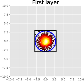
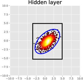
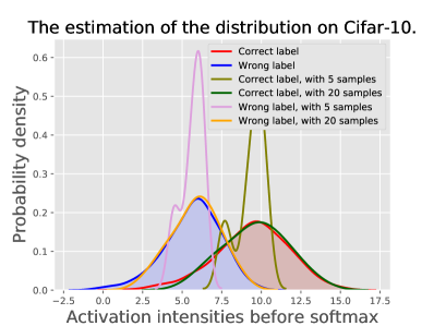
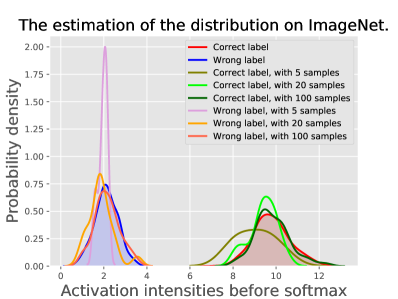
Figure 1: (a) Columns 1-3: Example of three methods for certifiable robustness on a two layers MLP. We show results of the input layer, hidden layer, and the output layer here. Black boxes based on using IBP [18]. Red dots come from the sampling idea from [56]. Ovals are covariance matrices if they are tracked exactly while considering interactions. (b) Columns 4-5: Example of Monte Carlo estimation on a different dataset. If the distributions of the correct and wrong labels are farther, the network is more robust. As the size of images grows, the number of samples for a good estimate also increases.

Recently, following the idea in [32, 30] at a high level, Cohen et al. [13] introduced an interesting randomized smoothing technique, which can be used to certify the robust radius $C_{R}$. Assume that we have a base network $f_{\theta}(\cdot)$ for classification. On a training image $\mathbf{x}\in\mathbb{R}^{d}$, the output $f_{\theta}(\mathbf{x})\in\mathcal{Y}$ is the predicted label of the image $\mathbf{x}$. Using $f_{\theta}(\cdot)$, we can build a “smoothed” neural network $g_{\theta}(\cdot)$.

$$g_{\theta}(\mathbf{x})=\operatorname*{arg\,max}_{c\in\mathcal{Y}}\mathbb{P}(f_{\theta}(\mathbf{x}+\boldsymbol{\varepsilon})=c),\text{where }\boldsymbol{\varepsilon}\sim\mathcal{N}(0,\sigma^{2}I)$$

Here, $\sigma$ can be thought of as a trade-off between the robustness and the accuracy of the smoothed classifier $g_{\theta}(\cdot)$. One can obtain a theoretical certified radius $C_{R}$ which states that when $||\boldsymbol{\delta}||_{2}\leq C_{R}$, the classifier $g_{\theta}(\mathbf{x}+\boldsymbol{\delta})$ will have same label $y$ as $g_{\theta}(\mathbf{x})$. MACER [56] nicely extended these ideas and also presented a differentiable form of randomized smoothing showing how it enables maximizing the radius. Internally, a sampling scheme is used, where empirically, the number of samples to get an accurate estimation could be large. As Fig. 1 (b) shows, one needs $100$ samples for a good estimation of the distribution of ImageNet.

Main intuition: MACER [56] showed that by sampling from a Gaussian distribution and softening the estimation of the distribution in the last layer, maximizing the certified radius is feasible. It is interesting to ask if tracking the “maximally perturbed” distribution directly – in the style of IBP – is possible without sampling. Results in [55] showed that the pre-activation vectors are i.i.d. Gaussian when the channel size goes to infinity. While unrealistic, it provides us a starting point. Since the Gaussian distribution can be fully characterized by the mean and the covariance matrix, we can track these two quantities as it passes through the network until the final layer, where the radius is calculated. If implemented directly, this scheme must involve keeping track of how pixel correlations influence the entries of the covariances from one layer to the next, and the bookkeeping needs grow rapidly. Alternatively, [55] uses the fixed point of the covariance matrix to characterize it while it passes through the network, but this idea is not adaptable for maximizing the radius task in [56]. We will use other convenient approximations of the covariance to make directly tracking of the distribution of the perturbation feasible.

Other applications of certified radius maximization: Training a robust network is also useful when training in the presence of noisy labels [1, 16, 41]. Normally, both crowd-sourcing from non-experts and web annotations, common strategies for curating large datasets introduce noisy labels. It can be difficult to train the model directly with the noisy labels without additional care [57]. Current methods either try to model the noise transition matrix [16, 41], or filter “correct” labels from the noisy dataset by collecting a consensus over different neural networks [19, 26, 35, 43]. This leads us to consider whether we can train the network from noisy labels without training any auxiliary network? A key observation here is that the margin of clean labels should be smoother than the noisy labels (as shown in Fig. 2).

Contributions: This paper shows how several known results characterizing the behavior of (and upper bounds on) covariance matrices that arise from interactions between random variables with known covariance structure can be leveraged to obtain a simple scheme that can propagate the distribution (perturbation applied to the training samples) through the network.

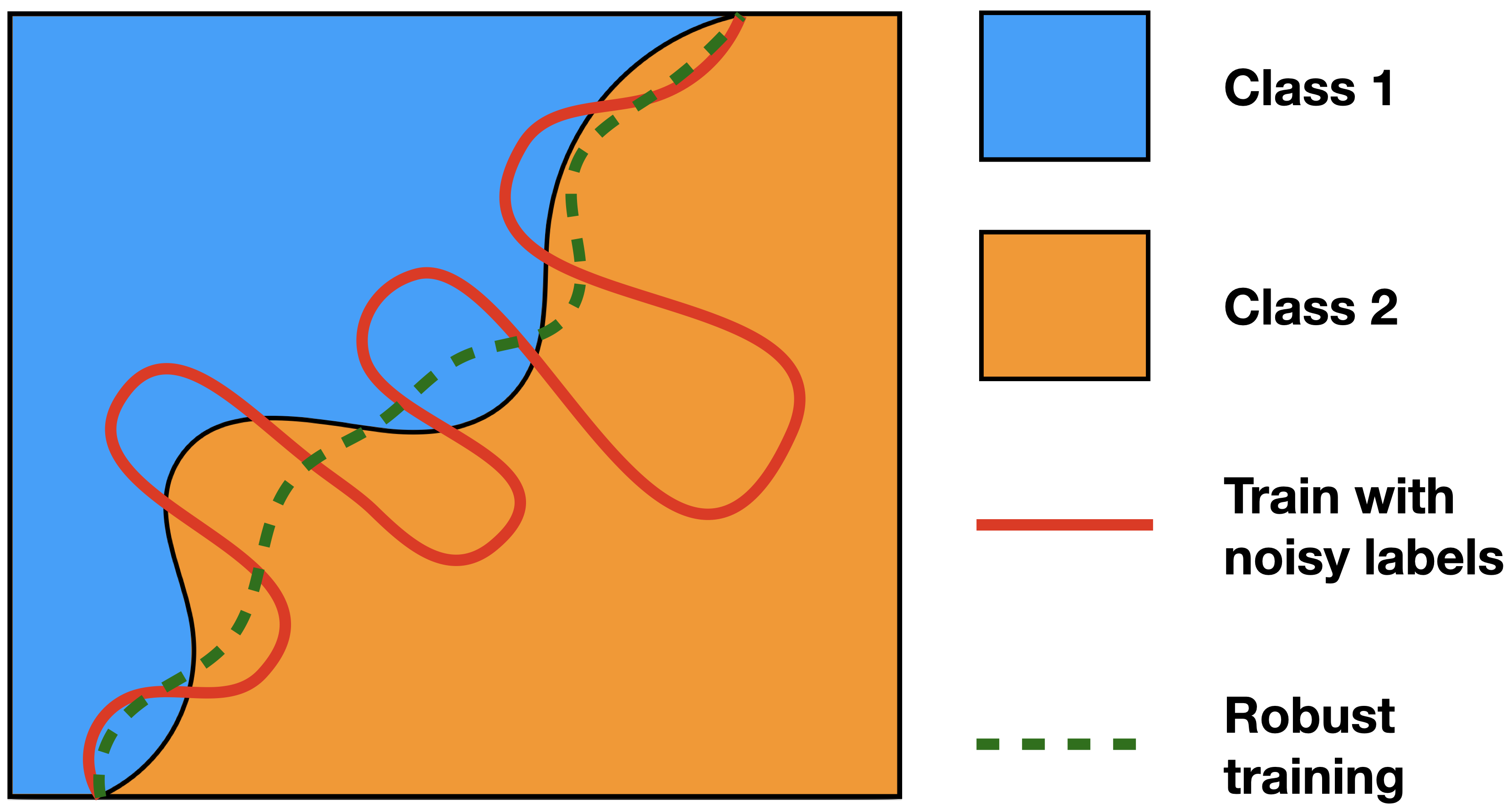
Figure 2: When directly training with noisy labels, the margin will resemble the red line. Using a robust network, the margin will resemble the green line.

This leads to a sampling-free method that performs favorably when compared to [56] and other similar approaches when the network depth is moderate. We show that our method is $5\times$ faster on Cifar-10 dataset and $1.5\times$ faster on larger datasets including ImageNet and Places365 relative to the current state-of-the-art without sacrificing much of the performance. Also, we show that the idea is applicable to or training with noisy labels.

2 Robust Radius Via Randomized Smoothing

We will briefly review the relevant background on robust radius calculation using Monte-Carlo (MC) sampling.
What is the robust radius? In order to measure the robustness of a neural network, the robust radius has been shown to be a sensible measure [52, 13]. Given a trained neural network $f_{\theta}$, the $\ell_{2}$-robustness at data point $(\mathbf{x},y)$ is defined as the largest radius $R$ of the ball centered at $\mathbf{x}$ such that all samples within the ball will be classified as $y$ by the neural network $f_{\theta}$. Analogously, the $\ell_{2}$-robustness of $f_{\theta}$ is defined as the minimum $\ell_{2}$-robustness at data point $(\mathbf{x},y)$ over the dataset. But calculating the robust radius for the neural network can be hard; [52] provides a hardness result for the $\ell_{1}$-robust radius. In order to make computing $\ell_{2}$-robustness tractable, the idea in [13] suggests working with a tight lower bound, called the “Certified Radius”, denoted by $0\leq C_{R}\leq R$. Let us now briefly review [13] its functions and features for a given base classifier $f_{\theta}(\cdot)$.

Note that we want to certify that there will be no adversarial samples within a radius of $C_{R}$. By smoothing out the perturbations $\boldsymbol{\varepsilon}$ around the input image/data $\mathbf{x}$ for the base classifier $f_{\theta}(\cdot)$, intuitively it will be harder to find an adversarial sample, since it will actually require finding a “region” of adversarial samples. If we can estimate a lower bound on the probability of the base classifier to correctly classify the perturbed data $\mathbf{x}+\boldsymbol{\varepsilon}$, denoted as $\underline{p_{c_{\mathbf{x}}}}$, as well as an upper bound of the probability of an incorrect classification $\overline{p_{\widetilde{c}}}\leq 1-\underline{p_{c_{\mathbf{x}}}}$, where $c_{\mathbf{x}}$ is the true label of $\mathbf{x}$ and $\widetilde{c}$ is the “most likely to be confused” incorrect label, a nice result for the smoothed classifier $g_{\theta}(\cdot)$ is available,

Theorem 1.

[13] Let $f_{\theta}:\mathbf{R}^{d}\rightarrow\mathcal{Y}$ be any deterministic or random function, and let $\boldsymbol{\varepsilon}\sim\mathcal{N}(\mathbf{0},\sigma^{2}I)$. Let $g_{\theta}$ be the randomized smoothing classifier defined as $g_{\theta}(\mathbf{x})=\operatorname*{arg\,max}_{c\in\mathcal{Y}}\mathbb{P}(f_{\theta}(\mathbf{x}+\boldsymbol{\varepsilon})=c_{\mathbf{x}})$. Suppose $c_{\mathbf{x}},\widetilde{c}\in\mathcal{Y}$ and $\underline{p_{c_{\mathbf{x}}}},\overline{p_{\widetilde{c}}}\in[0,1]$ satisfy $\mathbb{P}(f_{\theta}(\mathbf{x}+\boldsymbol{\varepsilon})=c_{\mathbf{x}})\geq\underline{p_{c_{\mathbf{x}}}}\geq\overline{p_{\widetilde{c}}}\geq\max_{\widetilde{c}\neq c_{\mathbf{x}}}\mathbb{P}(f_{\theta}(\mathbf{x}+\boldsymbol{\varepsilon})=\widetilde{c})$. Then $g_{\theta}(\mathbf{x}+\boldsymbol{\delta})=c_{\mathbf{x}}$ for all $\|\boldsymbol{\delta}\|_{2}<C_{R}$, where $C_{R}=\frac{\sigma}{2}(\Phi^{-1}(\underline{p_{c_{\mathbf{x}}}})-\Phi^{-1}(\overline{p_{\widetilde{c}}}))$.

The symbol $\Phi$ denotes the CDF of the standard Normal distribution. $\Phi$ and $\Phi^{-1}$ are involved because of smoothing the Gaussian perturbation $\boldsymbol{{\varepsilon}}$. The proof of this theorem can be found in [13]. We also include it in the appendix.

How to compute the robust radius? Using Theorem 3, we will need to compute the lower bound $\underline{p_{c_{\mathbf{x}}}}$, the main ingredient to compute $C_{R}$. In [13], the authors introduced a sampling-based method to compute the lower bound of $\underline{p_{c_{\mathbf{x}}}}$ in the test phase. The procedure first samples $n_{0}$ noisy samples around $\mathbf{x}$ and passes it through the base classifier $f_{\theta}$ to estimate the classified label after smoothing. Then, we sample $n$ noisy samples, where $n\gg n_{0}$, to estimate the lower bound of $\underline{p_{c_{\mathbf{x}}}}$ for a certain confidence level $\alpha$.

3 Track Distribution Approximately

In the last section, we discussed how to calculate $\underline{p_{c_{\mathbf{x}}}}$ in a sampling (Monte Carlo) based setting. However, this method is based on counting the number of correctly classified samples, which is not differentiable during training. In order to tackle this problem, [56] introduced an alternative – soft randomized smoothing – to calculate the lower bound

$$\underline{p_{c_{\mathbf{x}}}} =\mathbb{E}_{\boldsymbol{\varepsilon}\sim\mathcal{N}(\mathbf{0},\sigma^{2}I)}\left[\frac{e^{\beta u_{\theta}^{c_{\mathbf{x}}}(\mathbf{x}+\boldsymbol{\varepsilon})}}{\sum_{c^{\prime}\in\mathcal{Y}}e^{\beta u_{\theta}^{c^{\prime}}(\mathbf{x}+\boldsymbol{\varepsilon})}}\right]$$ (1)

where $u_{\theta}$ is the network $f_{\theta}$ without the last softmax layer, i.e., $f_{\theta}=\operatorname*{arg\,max}\text{softmax}(u_{\theta})$, and $\beta$ is a hyperparameter.

From Fig. 1 (b), observe that if we have enough MC samples, we can reliably estimate $\underline{p_{c_{\mathbf{x}}}}$ effectively by counting the number of correctly classified samples. If we can bypass MC sampling to estimate the final distribution, the gains in runtime can be significant. However, directly computing the joint distribution of the perturbations of all the pixels is infeasible: we need simplifying assumptions.

Gaussian pre-activation vectors: The first assumption is to use a Gaussian distribution to fit the pre-activation vectors. As briefly mentioned before, this is true when the channel size goes to infinity by the central limit theorem. In practice, when the channel size is large enough, e.g., a ResNet-based architecture [21], this assumption may be acceptable with a small error (evaluated later in experiments). Therefore, we will only consider the first two moments, which is reasonable for Gaussian perturbation [53].

Second moments: Our second assumption is that in each layer of a convolution network, the second moments are identical for the perturbation of all pixels. The input pixels share identical second moments from a fixed Gaussian perturbation $\varepsilon$. Due to weight sharing and the linearity of the convolution operators, the second moments will only depend on the kernel matrix without the position information. A more detailed discussion is in Obs. 4 and the appendix.

Notations and setup: Let $N$ be the number of channels. We use $\Sigma$ as the covariance matrices of the perturbation across the channels unless otherwise noted. The input perturbation comes from Gaussian perturbation $\varepsilon$ where $\Sigma=\sigma^{2}I$. As the image passes through the network, the input perturbation directly influences the output at each pixel as a function of the network parameters. We use $\Sigma_{i}\in\mathbf{R}^{N\times N}$, shorthand for $\Sigma_{\mathbf{x}_{i}}$, to denote the covariance of the perturbation distribution associated with pixel $i$ of image $\mathbf{x}$ denoted as $\mathbf{x}_{i}$. We call $\Sigma[i,j]$ as the $(i,j)$-entry of $\Sigma$. Notice that the $N$ changes from one layer to the other as the number of channels are different. So, the size of $\Sigma$ will change. Let $M_{q}$ be the number of pixels in the $q^{th}$ layer input, i.e., for $q=1$, $M_{1}$ is the number of pixels in the $1^{\text{st}}$ hidden layer of the network.

Similarly, $\boldsymbol{\mu}_{\mathbf{x}_{i}}$ or $\boldsymbol{\mu}_{i}\in\mathbf{R}^{N}$ is the mean of the distribution of the pixel $\mathbf{x}_{i}$ intensity after the perturbation. In the input layer, since the perturbation $\varepsilon\sim\mathcal{N}(0,\sigma^{2}I)$, $\boldsymbol{\mu}_{i}=\mathbf{x}_{i}$. At the $u_{\theta}$ layer, the number of channels is the number of classes, with the number of pixels being $1$. We use $\boldsymbol{\mu}[c_{\mathbf{x}}]$ and $\Sigma[c_{\mathbf{x}},c_{\mathbf{x}}]$ to denote the $c_{\mathbf{x}}$ component of $\boldsymbol{\mu}$ and $(c_{\mathbf{x}},c_{\mathbf{x}})$-entry of $\Sigma$ respectively. To denote the cross-correlation between two pixels $\mathbf{x}_{i},\mathbf{x}_{j}$, we use $E_{\mathbf{x}_{i}\mathbf{x}_{j}}$ or $E_{ij}\in\mathbf{R}^{N\times N}$. Note that this cross-correlation is across channels. For the special case with channel size $N=1$, we will use $\sigma^{(i)}\in\mathbf{R}$ to represent the variance in the $i^{\text{th}}$ layer. Let us define,

$$c_{\mathbf{x}}=\displaystyle\operatorname*{arg\,max}_{c\in\mathcal{Y}}\boldsymbol{\mu}[c],\quad\widetilde{c}=\displaystyle\operatorname*{arg\,max}_{{c}\in\mathcal{Y},{c}\neq c_{\mathbf{x}}}\boldsymbol{\mu}[c]$$ (2)

Let the number of classes $C=|\mathcal{Y}|$. Then, we can state the following.

Observation 1.

Using $u_{\theta}$, the prediction of the model can be written as $f_{\theta}(\mathbf{x})=\operatorname*{arg\,max}_{c\in\mathcal{Y}}\text{ softmax}(u_{\theta}(\mathbf{x}))$. Assume $u_{\theta}(\mathbf{x})\sim\mathcal{N}(\boldsymbol{\mu},\Sigma)$, where $\mathbf{x}\sim\mathcal{N}(\boldsymbol{\mu}_{\mathbf{x}},\Sigma_{\mathbf{x}})$, $\boldsymbol{\mu}\in\mathbf{R}^{C}$ and $\Sigma\in\mathbf{R}^{C\times C}$. Then the estimation of $\underline{p_{c_{\mathbf{x}}}}$ is

$$\underline{p_{c_{\mathbf{x}}}} =\Phi(\frac{\boldsymbol{\mu}[{c_{\mathbf{x}}}]-\boldsymbol{\mu}[{\widetilde{c}}]}{\sqrt{\Sigma[{c_{\mathbf{x}},c_{\mathbf{x}}}]+\Sigma[{\widetilde{c},\widetilde{c}}]-2\Sigma[{c_{\mathbf{x}},\widetilde{c}}]}})$$ (3)

Notice that propagating $\boldsymbol{\mu}$ through the network is simple, since tracking the mean is the same as directly passing it through the network when there is no nonlinear activation, and requires no cross-correlation between pixels. But tracking $\Sigma$ at each step of the network can be challenging and some approximating techniques have been used in literature for simple networks [45]. To see this, let us consider a simple 1-D example.

Bookkeeping problem: Consider a simple 1-D convolution with a kernel size $k$. By Obs. 3, we will need the distribution of $u_{\theta}(\mathbf{x})$ of the $i^{th}$ layer (i.e., the network without the softmax layer). Directly, this will involve taking into account $k^{1}$ pixels in the $(i-1)^{th}$ layer, and $k^{2}$ pixels in the $(i-2)^{th}$ layer. We must calculate the covariance $\Sigma$ and also calculate the cross-correlation $E$ between all $k^{q}$ pixels in $(i-q)^{th}$ layer. This trend stops when we hit $k^{q}>M_{i-q}$, where $M_{i-q}$ is the number of pixels at $(i-q)$ layer, but it is impractical anyway.

If we temporarily assume that the network involves no activation functions, and if the input perturbation is identical for all pixels, then the variance of all pixels after perturbation is also identical. Thus, the variance of each pixel only relies on the variance of the perturbation and not on the pixel intensity. This may allow us to track one covariance matrix instead of $M$ for all $M$ pixels.

Observation 2.

With the input perturbation $\boldsymbol{\varepsilon}$ set to be identical along the spatial dimension and without nonlinear activation function, for $q^{th}$ hidden convolution layer with $\{\mathbf{h}_{i}\}_{i=1}^{M_{q}}$ output pixels, we have $\Sigma_{\mathbf{h}_{i}}^{(q)}=\Sigma_{\mathbf{h}_{j}}^{(q)},\forall i,j\in\{1,\cdots,M_{q}\}$.

The Obs. 4 only reduces the cost marginally: instead of computing all the covariances of the perturbation for all pixels, $\Sigma_{1}^{(i-q)},\Sigma_{2}^{(i-q)},\cdots,\Sigma_{k}^{(i-q)}$, we only need to compute a single $\Sigma^{(i-q)}$. Unfortunately, we still need to compute all different $E_{ij}^{(i-2)}$ that will contribute to $u_{\theta}(\mathbf{x})$ (also see worked out example in the appendix). Thus, due to these cross-correlation terms $E_{ij}$, the overall computation is still not feasible. In any case, the assumption itself is unrealistic: we do need to take nonlinear activations into account which will break the identity assumption of the second moments. For this reason, we explore a useful approximation which we discuss next.

3.1 How To Make Distribution Tracking Feasible

From the previous discussion, we observe that a key bottleneck of tracking distribution across layers is to track the interaction between pairs of pixels, i.e., cross-correlations. Thus, we need an estimate of the cross-correlations between pixels. In [20], the authors provide an upper-bound on the joint distribution of two multivariate Gaussian random variables such that the upper bounding distribution contains no cross-correlations. This result will be crucial for us.

Formally, let $\mathbf{x}_{1},\mathbf{x}_{2}\in\mathbf{R}^{N}$ be two random vectors representing two pixels with $N$ channels. Without any loss of generalization, assume that $\mathbf{x}_{1}\sim\mathcal{N}(\mathbf{0},\Sigma_{1})$, and $\mathbf{x}_{2}\sim\mathcal{N}(\mathbf{0},\Sigma_{2})$ (if the mean is not $\mathbf{0}$, we can subtract the mean without affecting the covariance matrix). Also, assume that we do not know the cross-correlation between $\mathbf{x}_{1}$ and $\mathbf{x}_{2}$, i.e., ${E}_{12}$. Instead, the correlation coefficient $r$ is bounded by $r_{max}$, i.e., $|r|\leq r_{max}$.

With the above assumptions, we can bound the covariance matrix of the joint distribution of two $N$-dimensional random vectors ${\mathbf{x}_{1}},{\mathbf{x}_{2}}$ by two independent random vectors $\widehat{\mathbf{x}_{1}},\widehat{\mathbf{x}_{2}}$. We will use the notation “ $\widehat{\cdot}$ ” to denote the upper bound estimation of “$\cdot$”. The upper bound here means that $[\widehat{\Sigma}-\Sigma]$ is a positive semi-definite matrix, where $\widehat{\Sigma}$ is the joint distribution of the two independent random vectors $\widehat{\mathbf{x}_{1}}$ and $\widehat{\mathbf{x}_{2}}$. Here, $\Sigma$ is the joint distribution of ${\mathbf{x}_{1}},{\mathbf{x}_{2}}$ with correlation. Formally,

Theorem 2.

[20] When $\widehat{\mathbf{x}_{1}}\sim\mathcal{N}(\mathbf{0},\widehat{\Sigma_{1}}=\tau_{1}\Sigma_{1})$, and $\widehat{\mathbf{x}_{2}}\sim\mathcal{N}(\mathbf{0},\widehat{\Sigma_{2}}=\tau_{2}\Sigma_{2})$, the covariance matrix $\mathbf{B}=\widehat{\Sigma}=\begin{bmatrix}\tau_{1}\Sigma_{1}&0\\ 0&\tau_{2}\Sigma_{2}\end{bmatrix}$ bounds the joint distribution of $\mathbf{x}_{1}$ and $\mathbf{x}_{2}$, i.e., $\mathbf{B}\succeq\Sigma=\begin{bmatrix}\Sigma_{1}&E_{12}\\ E_{21}&\Sigma_{2}\end{bmatrix}$, where $\tau_{1}=\frac{1}{\eta-\kappa}$, $\tau_{2}=\frac{1}{\eta+\kappa}$, $\kappa^{2}\leq\frac{1-2\eta}{1-r_{max}^{2}}+\eta^{2}$, and $0.5\leq\eta\leq\frac{1}{1+r_{max}}$.

With this result in hand, we now discuss how to use it to makes the tracking of moments across layers feasible.
How to use Theorem 2? By Obs. 4, we can store one covariance matrix over the convolved output pixels at each layer. Notice that due to the presence of the cross-correlation between output pixels, we also need to store cross-correlation matrices, which was our bottleneck! But with the help of Theorem 2, we can essentially construct independent convolved outputs, called $\left\{\widehat{\mathbf{h}_{i}}\right\}$, that bound the covariance of the original convolved outputs, $\left\{\mathbf{h}_{i}\right\}$. To apply this theorem, we need to estimate the bounding covariance matrix $\mathbf{B}$, which can be achieved with the following simple steps (the notations are consistent with Theorem 2)

1. We estimate the bound on correlation coefficient $r_{max}$

2. Assign $\eta=\frac{1}{1+r_{max}}$

3. Assign $\kappa=0$ which essentially implies $\tau_{1}=\tau_{2}$

Remark: When computing the variance $\Sigma[{c_{\textbf{x}},c_{\textbf{x}}}]$ in the $i^{th}$ layer, we need only $k$ upper bound of covariances $\widehat{\Sigma_{1}}^{(i-1)},\widehat{\Sigma_{2}}^{(i-1)},\cdots,\widehat{\Sigma_{k}}^{(i-1)}$ from the $(i-1)^{th}$ layer. Moreover, using the assumption that the covariance matrices of the $(i-1)^{\text{th}}$ layers to be identical across pixels when the input perturbation is identical, we only compute $\widehat{\Sigma}^{(i-1)}$, which in turn requires computing only one upper bound of covariance. Hence, the computational cost reduces to linear in terms of the depth of the network.

Ansatz: The assumption of identical pixels (when removing the mean) is sensible when the network is linear. But the assumption is undesirable. So, we will need a mechanism to deal with the nonlinear activation function setting. Further, we will need to design the mechanics of how to track the mean and covariance for different type of layers. We will describe the details next.

3.2 Robust Training By Propagating Covariances

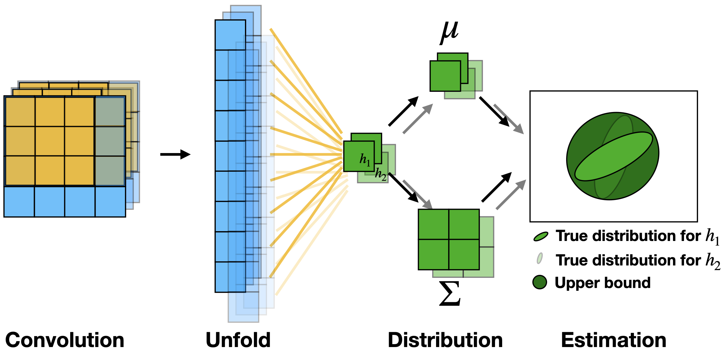
Figure 3: (a) Left: The LeNet with tracking the bounding box or the covariance matrices over each layer. The covariance matrices are denoted as the ovals. Since bounding boxes are proportional to $||W||_{1}$, while covariance matrices are proportional to $||W||_{2}$, the covariance-based upper bound will be tighter than the box-base one. (b) Right: The yellow blocks are the kernel of convolution, while the blue blocks are the data. After computing the distribution, we use an upper bound to remove the dependency of two pixels $h_{1},h_{2}$.

Overview: We described simplifying the computation cost by tracking the upper bounds on the perturbation of the independent pixels. We introduce details of an efficient technique to track the covariance of the distribution across different types of layers in a CNN. We will also describe how to deal with nonlinear activation functions.

We treat the $i^{th}$ pixel, after perturbation, as drawn from a Gaussian distribution $\mathbf{x}_{i}\sim\mathcal{N}(\boldsymbol{\mu}_{i},\Sigma)$, where $\boldsymbol{\mu}_{i}\in\mathbf{R}^{N}$ and $\Sigma$ is the covariance matrix across the channels (note that $\Sigma$ is the same across pixels for the same layer). We may remove the indices to simplify the formulation and avoid clutter. A schematic showing propagating the distribution across LeNet [7] model, for simplicity, is shown in Fig. 3(a) denoted by the colored ovals.

To propagate the distribution through the whole network, we need a way to propagate the moments through the layers, including commonly used network modules, such as convolution and fully connected layers. Since the batch normalization layer normally has a large Lipschitz constant, we do not include the batch normalization layer in the network. We will introduce the high-level idea, while the low-level details are in the appendix.

Convolution layer: Since the convolution layer is a linear operator, the covariance of an output pixel $\Sigma_{\mathbf{h}}\in\mathbf{R}^{N_{out}\times N_{out}}$ is defined as $\Sigma_{\mathbf{h}}=W^{T}\widetilde{\Sigma}W$. Here, let $\widetilde{\mathbf{x}}\in\mathbf{R}^{N_{in}k^{2}}$ be the vector consisting of all the independent variables inside a $k\times k$ kernel $\{\mathbf{x}_{i}\}$, $\widetilde{\Sigma}\in\mathbf{R}^{N_{in}k^{2}\times N_{in}k^{2}}$ is the covariance of the concatenated $\widetilde{\mathbf{x}}$. $W$ is the reshaped weight matrix of the shape $N_{in}k^{2}\times N_{out}$.

We need to apply Theorem 2 to compute the upper bound of $\Sigma_{\mathbf{h}}$ as $\widehat{\Sigma_{\mathbf{h}}}=(1+r_{max})W^{T}\widetilde{\Sigma}W$ to avoid the computational costs of the dependency from cross-correlations. A pictorial description of propagating moments through the convolution layer is shown in Fig. 3(b).

First (and other) linear layers: The first linear layer can be viewed as a special case of convolution with kernel size equal to the input spatial dimension. Since there will only be one output neuron $\mathbf{h}$ (with channels), there is no need to break the cross-correlation between neurons. Thus, $\Sigma_{\mathbf{h}}=W^{T}\Sigma_{\mathbf{\widetilde{x}}}W$ and takes a form similar to the convolution layer.

Special case: From Obs. 3, we only need the largest two intensities to estimate the $\underline{p_{c_{\mathbf{x}}}}$ in the $u_{\theta}(\mathbf{x})$ layer. Thus, if there is only one linear layer as the last layer in the $u_{\theta}(\mathbf{x})$, as in most of ResNet like models, this can be further simplified. We only need to consider the covariance matrix between $c_{\mathbf{x}}$ and $\widetilde{c}$ index of $u_{\theta}(\mathbf{x})$. Thus, this will need calculating a $2\times 2$ covariance matrix instead of a $C\times C$ matrix.

On the other hand, if the network consists of multiple linear layers, calculating the moments of the subsequent linear layers must be handled differently. Let $\mathbf{x}\sim\mathcal{N}\left(\boldsymbol{\mu}^{(i)}_{\mathbf{x}},\Sigma^{(i)}_{\mathbf{x}}\right)\in\mathbf{R}^{N_{i}}$ be the input of the $i^{th}$ linear layer given by $\mathbf{h}=W_{i}^{T}\mathbf{x}+\mathbf{b}_{i}$, then

$$\mathbf{h}\sim\mathcal{N}\left(W_{i}^{T}\boldsymbol{\mu}^{(i)}_{\mathbf{x}}+\mathbf{b}_{i},W_{i}^{T}\Sigma^{(i)}_{\mathbf{x}}W_{i}\right).$$

Here, $W_{i}\in\mathbf{R}^{N_{i}\times N_{i+1}}$, $\mathbf{b}_{i}\in\mathbf{R}^{N_{i+1}}$, and $\mathbf{h}\in\mathbf{R}^{N_{i+1}}$.

Pooling layer: Recall that the input of a max pooling layer is $\{\mathbf{x}_{i}\}$ where each $\mathbf{x}_{i}\in\mathbf{R}^{N_{in}}$ and the index $i$ varies over the spatial dimension. Observe that as we identify each $\mathbf{x}_{i}$ by the respective distribution $\mathcal{N}\left(\boldsymbol{\mu}_{i},\Sigma\right)$, applying max pooling over $\mathbf{x}_{i}$ essentially requires computing the maximum over $\left\{\mathcal{N}\left(\boldsymbol{\mu}_{i},\Sigma\right)\right\}$, which is not a well-defined operation. Thus, we restrict ourselves to average pooling. This can be viewed as a special case of the convolution layer with no overlapping and the fixed kernel: $\mathbf{h}\sim\mathcal{N}\left(\frac{1}{k^{2}}\sum_{\mathbf{x}_{i}\in\mathbb{W}}\boldsymbol{\mu}_{i},\frac{\Sigma}{k^{2}}\right)$, $\mathbb{W}$ is the kernel window.

Normalization layer: For the normalization layer, given by $\mathbf{h}=(\mathbf{x}-\mu^{\prime})/\sigma^{\prime}$, where $\mu^{\prime},\sigma^{\prime}$ can be computed in different ways [25, 4, 51], we have $\mathbf{h}\sim\mathcal{N}\left((\boldsymbol{\mu}^{(i)}_{\mathbf{x}}-\mu^{\prime})/\sigma^{\prime},\Sigma^{(i)}_{\mathbf{x}}/\sigma^{\prime 2}\right)$. However, as the normalization layers often have large Lipschitz constant [3], we omit these layers in this work.

Activation layer: This is the final missing piece in efficiently tracking the moments. The overall goal is to find an identical upper bound of the second moments after the activation layer when the input vectors share identical second moments. Also, the first moments should be easier to compute, and ideally, will have a closed form. In [8, 31], the authors introduced a scheme to compute the mean and variance after a ReLU operation. Since ReLU is an element-wise operation, for each element (a scalar), assume $x\sim\mathcal{N}(\mu,\sigma^{2})$. After ReLU activation, the first and second moments of the output are given by:

$$\mathbb{E}(\text{ReLU}(x)) =\frac{1}{2}\mu-\frac{1}{2}\mu\ \textsf{erf}(\frac{-\mu}{\sqrt{2}\sigma})+\frac{1}{\sqrt{2\pi}}\sigma\exp(-\frac{\mu^{2}}{2\sigma^{2}}),$$

$$\text{var}(\text{ReLU}(x)) <\text{var}(x)$$

Here, erf is the Error function. Since we want an identical upper bound of the covariance matrix after ReLU, as well as the closed form of the mean, we use $\text{ReLU}(\mathbf{x})\sim\mathcal{N}\left(\boldsymbol{\mu}_{a},\Sigma_{a}\right)$ where,

$$\boldsymbol{\mu}_{a} =\frac{1}{2}\boldsymbol{\mu}-\frac{1}{2}\boldsymbol{\mu}\ \textsf{erf}(\frac{-\boldsymbol{\mu}}{\sqrt{2}\boldsymbol{\sigma}})+\frac{1}{\sqrt{2\pi}}\boldsymbol{\sigma}\exp(-\frac{\boldsymbol{\mu}^{2}}{2\boldsymbol{\sigma}^{2}}),$$

$$\Sigma_{a} \preceq\Sigma$$

$\boldsymbol{\sigma}$ is the square root of the diagram of $\Sigma$, $\boldsymbol{\mu}$ is the mean of the input vector. All the operators in the first equation are element-wise operators.

Last layer/prediction: The last layer is the layer before softmax layer, which represents the “strength” of the model for a specific class. By Obs. 3, we have the estimate

$$p_{c_{\mathbf{x}}}=\underline{p_{c_{\mathbf{x}}}}=\Phi\left(\frac{\boldsymbol{\mu}[{c_{\mathbf{x}}}]-\boldsymbol{\mu}[{\widetilde{c}}]}{\sqrt{\Sigma[{{c_{\mathbf{x}}},{c_{\mathbf{x}}}}]+\Sigma[{\widetilde{c},\widetilde{c}}]-2\Sigma[{{c_{\mathbf{x}}},\widetilde{c}}]}}\right)$$

and $p_{\widetilde{c}}=\overline{p_{\widetilde{c}}}=1-p_{c_{\mathbf{x}}}$ as an upper bound estimation. By Theorem 3, the certified radius is

$$C_{R}= \frac{\sigma}{2}(\Phi^{-1}(\underline{p_{c_{\mathbf{x}}}})-\Phi^{-1}(\overline{p_{\widetilde{c}}}))$$ (4)

$$= \sigma\frac{\boldsymbol{\mu}[c]-\boldsymbol{\mu}[{\widetilde{c}}]}{\sqrt{\Sigma[{{c_{\mathbf{x}}},{c_{\mathbf{x}}}}]+\Sigma[{\widetilde{c},\widetilde{c}}]-2\Sigma[{{c_{\mathbf{x}}},\widetilde{c}}]}}.$$ (5)

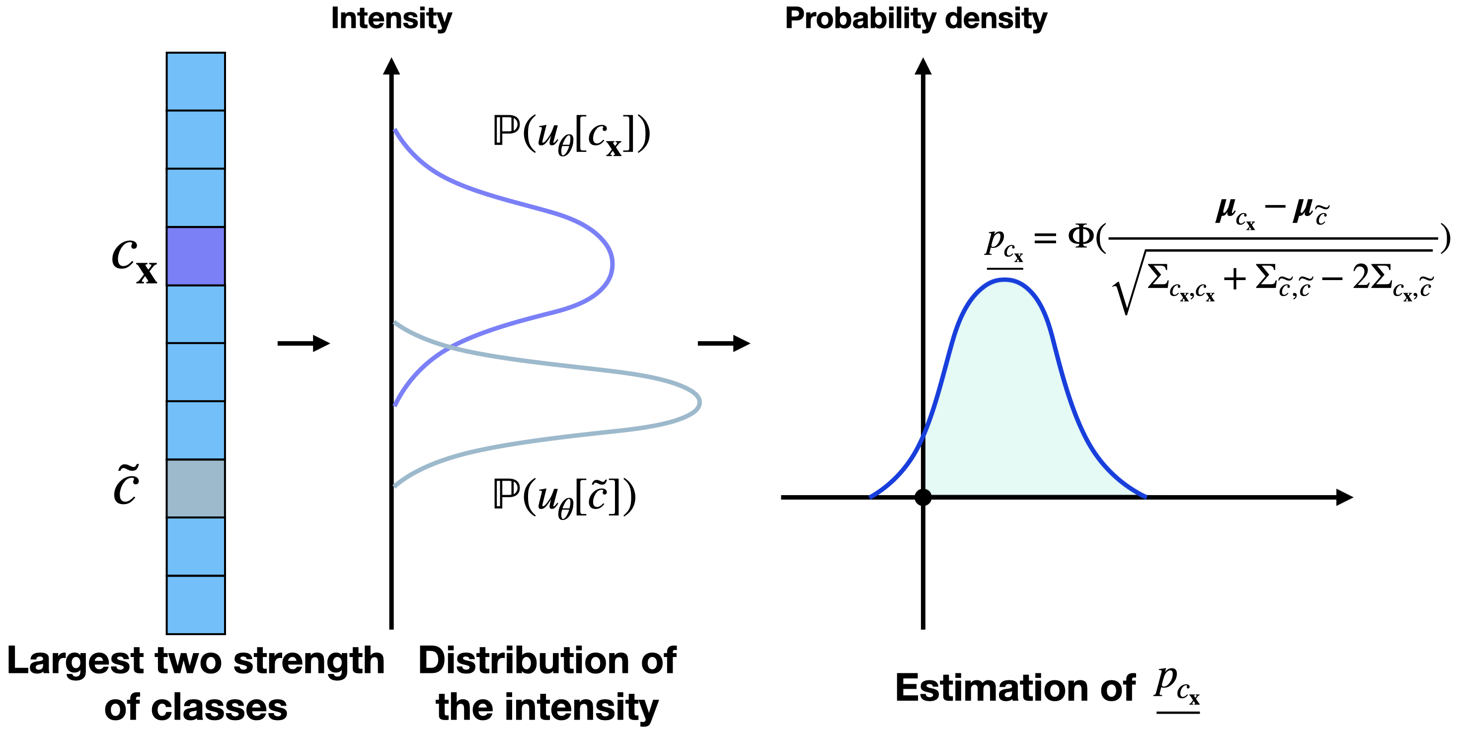
Figure 4: In the last layer, we first find the indexes of the largest two intensity ${c_{\mathbf{x}}},\widetilde{c}$. Then compute the $\underline{p_{c_{\mathbf{x}}}}$.

Network structures used: In the experiment, we applied two types of network on different dataset, LeNet [7] and PreActResnet-18 [22].

LeNet requires convolution layer, average pooling layer, activation layer, and linear layer. We build the network with three convolution layers with activation and pooling after each layer, and two linear layers.

The structure of PreActResnet-18 is similar with two major differences – the residual connection and it involves only one linear layer. For the residual connection, it can be viewed as a special type of linear layer. Due to the assumption of independence, the final covariance is the addition of two inputs. Also, there is only one linear layer as the final layer. Thus, we can reduce the cost of computing the whole covariance matrix to only computing the covariance matrix of the largest two intensities.

As discussed above, we removed all batch normalization layers within the network as well as replaced all max pooling operations to the average pooling layer in the network structure. Our experiments suggest that there is minimal impact on performance.

Table 1: A review of different layers. Here, $\boldsymbol{\mu}_{i},\Sigma_{i}$ is the mean and covariance matrix of the input channels, while $\boldsymbol{\mu}_{o},\Sigma_{o}$ is the mean and covariance after that layer.

	Convolution	Linear	Pooling	Activation
$\boldsymbol{\mu}_{o}$	$conv(\boldsymbol{\mu}_{i},W)+b$	$W^{T}\boldsymbol{\mu}_{i}+b$	$\frac{1}{k^{2}}\sum\boldsymbol{\mu}_{i}$	$\frac{1}{2}\boldsymbol{\mu}_{i}-\frac{1}{2}\boldsymbol{\mu}_{i}\ \textsf{erf}(\frac{-\boldsymbol{\mu}_{i}}{\sqrt{2}\boldsymbol{\sigma}})$
				$+\frac{1}{\sqrt{2\pi}\boldsymbol{\sigma}}\exp(-\frac{\boldsymbol{\mu}_{i}^{2}}{2\boldsymbol{\sigma}^{2}})$
$\Sigma_{o}$	$(1+r_{max})W^{T}\widetilde{\Sigma_{i}}W$	$W^{T}{\Sigma_{i}}W$	$\frac{1}{k^{2}}\Sigma_{i}$	$\Sigma_{i}$

3.3 Training Loss

In the spirit of [56], the training loss consists of two parts: the classification loss and the robustness loss, i.e., the total loss $l(g_{\theta};\mathbf{x},y)=l_{C}(g_{\theta};\mathbf{x},y)+\lambda l_{C_{R}}(g_{\theta};\mathbf{x},y)$. Similar to the literature, we use the softmax layer on the expectation to compute the cross-entropy of the prediction and the true label, given by

$$l_{C}(g_{\theta};\mathbf{x},y)=y\log(\text{softmax}(\mathbb{E}[u_{\theta}(\mathbf{x})]))$$

Here, $l_{C_{R}}(g_{\theta};\mathbf{x},y=c_{\mathbf{x}})$ is

$$\max(0,\Gamma-\sigma\frac{\boldsymbol{\mu}[c_{\mathbf{x}}]-\boldsymbol{\mu}[{\widetilde{c}}]}{\sqrt{\Sigma[{c_{\mathbf{x}},c_{\mathbf{x}}}]+\Sigma[{\widetilde{c},\widetilde{c}}]-2\Sigma[{c_{\mathbf{x}},\widetilde{c}}]}})$$

Thus, minimizing the loss of $l_{C_{R}}$ is equivalent to maximizing $C_{R}$. $\Gamma$ is the offset to control the certified radius.

4 Experiments

In this section, we discuss the applicability and usefulness of our proposed model in two applications namely (a) image classification tasks to show the performance of our proposed model both in terms of performance and speed (b) trainability of our model on data with noisy labels.

4.1 Robust Training

Similar to [13], we use the approximate certified test set accuracy as our metric, which is defined as the percentage of test set whose $C_{R}\leq r$. For a fair comparison, we use the Monte Carlo method introduced in [13] Section 3.2 to compute $C_{R}$ here just as our baseline model does. Recall that $C_{R}=0$ if the classification is wrong. Otherwise, $C_{R}=\sigma\Phi^{-1}(\underline{p_{A}})$ (please refer to the pseudocode in [13]). In order to run certification, we used the code provided by [13]. We also report the average certified radius (ACR), which is defined as $\frac{1}{m}\sum_{i=1}^{m}C_{R}(\mathbf{x}^{i})$ over the test set.

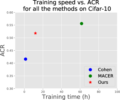
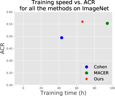
Figure 5: The training speed for three models on Cifar-10 and ImageNet dataset, including [13], MACER [56], and ours.

Datasets and baselines: We evaluate our proposed model on five vision datasets: MNIST [29], SVHN [38], Cifar-10 [28], ImageNet [14], and Places365 [61]. We modify LeNet for MNIST dataset and PreActResnet-18 [22] for SVHN, Cifar-10, ImageNet, and Places365 datasets similarly as in [13]. Our baseline model is based on Monte Carlo samples, which requires a large number of samples to make an accurate estimation. In the rest of the section, we will observe that our model can be at best $5\times$ faster than the baseline model. For the larger dataset, since MACER [56] uses a reduced number of MC samples, our model is $1.5\times$ faster.
Model hyperparameters: During training, we use a similar strategy as our baseline model. We train the base classifier first and then fine-tune our model considering the aforementioned robust error. We train a total of $200$ epochs with the initial learning rate to be $0.01$ for MNIST, SVHN, and Cifar-10. The learning rate decays at $100,150$ epochs respectively. The $\lambda$ is set to be $0$ in the initial training step, and changes to $4.0$ at epoch $100$ for MNIST, SVHN, and Cifar-10. For ImageNet and Places365 dataset, we train 120 epochs with $\lambda$ being 0.5 after 30 epochs. The initial learning rate is $0.01$ and decays linearly at $30,60,90$ epochs.
Results: We report the numerical results in Table. 3, where, the number reported in each column represents the ratio of the test set with the certified radius larger than the header of that column. Thus, the larger the number is, the better the performance of different models. The ACR is the average of all the certified radius on the test set. Note that the certified radius is $0$ when the classification result is wrong. It is noticeable that our model strikes a balance of robustness and the training speed. We achieve $5\times$ speed-up over [56], which uses the Monte Carlo method during the training phase, as shown in Fig. 5. On the other hand, compared with [13], our model achieves competitive accuracy and certified radius. We like to point out that although SmoothAdv [44] is a powerful model, we did not compare with SmoothAdv because MACER [56] performs better than SmoothAdv [44] in terms of ACR and training speed.

Table 2: Statistics for different layers of MC sampling and our upper bound tracking method.

Layer number	1	5	9	13	17
MC (1000 samples)	0.243	0.913	2.740	2.999	0.712
Upper bound	0.256	1.126	4.069	5.367	1.208

Separate from the quantitative performance measures, we also evaluate the validity of Gaussian assumption on the pre-activation vectors within the network. Here, we choose PreActResNet-18 on ImageNet to visualize the first two channels across different layers. The detailed results are shown in Fig. 6 and Table. 2. These results not only show that the assumption is reasonable along the neural network, but also demonstrates that our method can estimate the covariance matrix well when the depth of network is moderate. Deeper networks, where the bounds get looser, are described in the appendix.

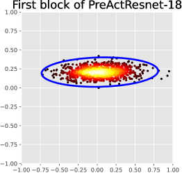
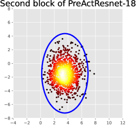
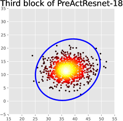
Figure 6: A visualization of the first two channels within the neural network across different layers. The dots are the actual MC samples and the color represents the density at that point. The blue oval is generated from the covariance matrices we are tracking.

Ablation study: We perform an ablation study on the choice of the hyperparameters for Places365 dataset. We fix $\sigma$ of the perturbation to be $0.5$. We first test the influence of $\lambda$ which is the balance between the accuracy (first moments) and the robustness (second moments). Also, to verify the estimation of $r_{max}$, we tried different $r_{max}$ estimates while fixing $\lambda=0.5$. The detailed results are shown in Table. 4.

Discussion: A key benefit of our method is the training time. As shown in Fig. 5, our method can be $5\times$ faster on Cifar-10, dataset, with a comparable ACR as MACER. For larger datasets, since MACER reduces the number of MC samples in their algorithm, our method is only $1.5\times$ faster with a slightly better ACR than MACER. Hence, our method is a cheaper substitute of the SOTA with a marginal performance compromise.

Table 3: The results on MNIST, SVHN, Cifar-10, ImageNet, and Places365 with the certified robustness. The number reported in each column represents the ratio of the test set with the certified radius larger than the header of that column under the perturbation $\sigma$. ACR is the average certified radius of all the test samples. A larger value is better for all the numbers reported.

Dataset	$\sigma$	Method	0.00	0.25	0.50	0.75	1.00	1.25	1.50	1.75	ACR
MNIST	0.25	Cohen [13]	0.99	0.97	0.94	0.89	0	0	0	0	0.887
		MACER [56]	0.99	0.99	0.97	0.95	0	0	0	0	0.918
		Ours	0.99	0.98	0.96	0.92	0	0	0	0	0.904
	0.50	Cohen [13]	0.99	0.97	0.94	0.91	0.84	0.75	0.57	0.33	1.453
		MACER [56]	0.99	0.98	0.96	0.94	0.90	0.83	0.73	0.50	1.583
		Ours	0.98	0.98	0.95	0.91	0.87	0.77	0.62	0.37	1.485
SVHN	0.25	Cohen [13]	0.90	0.70	0.44	0.26	0	0	0	0	0.469
		MACER [56]	0.86	0.72	0.56	0.39	0	0	0	0	0.540
		Ours	0.89	0.68	0.48	0.36	0	0	0	0	0.509
	0.50	Cohen [13]	0.67	0.48	0.37	0.24	0.14	0.08	0.06	0.03	0.434
		MACER [56]	0.61	0.53	0.44	0.35	0.24	0.15	0.09	0.04	0.538
		Ours	0.67	0.53	0.36	0.29	0.19	0.12	0.07	0.03	0.475
Cifar-10	0.25	Cohen [13]	0.75	0.60	0.43	0.26	0	0	0	0	0.416
		MACER [56]	0.81	0.71	0.59	0.43	0	0	0	0	0.556
		Ours	0.80	0.72	0.55	0.37	0	0	0	0	0.518
	0.50	Cohen [13]	0.65	0.54	0.41	0.32	0.23	0.15	0.09	0.04	0.491
		MACER [56]	0.66	0.60	0.53	0.46	0.38	0.29	0.19	0.12	0.726
		Ours	0.58	0.56	0.43	0.36	0.27	0.15	0.08	0.01	0.543

Dataset	$\sigma$	Method	0.00	0.25	0.50	0.75	1.00	1.25	1.50	1.75	ACR
ImageNet	0.25	Cohen [13]	0.58	0.49	0.40	0.29	0	0	0	0	0.379
		MACER[56]	0.59	0.52	0.43	0.34	0	0	0	0	0.418
		Ours	0.64	0.55	0.44	0.33	0	0	0	0	0.425
	0.50	Cohen [13]	0.43	0.38	0.34	0.29	0.26	0.22	0.17	0.12	0.494
		MACER [56]	0.54	0.47	0.39	0.32	0.29	0.21	0.17	0.11	0.553
		Ours	0.52	0.47	0.39	0.32	0.28	0.23	0.18	0.13	0.560
	1.00	Cohen [13]	0.21	0.19	0.18	0.16	0.15	0.13	0.11	0.09	0.345
		MACER [56]	0.37	0.33	0.30	0.26	0.22	0.19	0.15	0.12	0.517
		Ours	0.38	0.33	0.29	0.26	0.22	0.19	0.15	0.11	0.519
Places365	0.25	Cohen [13]	0.45	0.42	0.36	0.29	0	0	0	0	0.340
		MACER[56]	0.46	0.44	0.39	0.30	0	0	0	0	0.359
		Ours	0.50	0.46	0.40	0.33	0	0	0	0	0.380
	0.50	Cohen [13]	0.43	0.38	0.35	0.28	0.23	0.19	0.17	0.12	0.484
		MACER [56]	0.45	0.42	0.37	0.31	0.26	0.22	0.18	0.13	0.533
		Ours	0.46	0.43	0.39	0.35	0.31	0.28	0.23	0.16	0.597
	1.00	Cohen [13]	0.20	0.18	0.16	0.15	0.13	0.12	0.11	0.10	0.357
		MACER [56]	0.31	0.29	0.28	0.25	0.22	0.21	0.19	0.17	0.615
		Ours	0.32	0.30	0.29	0.26	0.24	0.21	0.19	0.16	0.622

Table 4: Ablation experiment on Places365 with $\sigma=0.5$. We perform the choice of $\lambda$ and $r_{max}$ as the hyper-parameters.

Parameters	Value	0.00	0.25	0.50	0.75	1.00	1.25	1.50	1.75	ACR
$\lambda$	0.0	0.43	0.38	0.35	0.28	0.23	0.19	0.17	0.12	0.484
	0.5	0.47	0.44	0.39	0.34	0.29	0.23	0.19	0.14	0.565
	1.0	0.44	0.41	0.34	0.30	0.28	0.23	0.20	0.14	0.530
$r_{max}$	0.0	0.43	0.38	0.36	0.31	0.27	0.21	0.16	0.13	0.509
	0.1	0.47	0.44	0.39	0.34	0.29	0.23	0.19	0.14	0.565
	0.2	0.46	0.43	0.39	0.35	0.31	0.28	0.23	0.16	0.597
	0.3	0.46	0.44	0.41	0.35	0.29	0.23	0.19	0.15	0.573
	0.4	0.44	0.40	0.36	0.31	0.27	0.23	0.17	0.12	0.520

Table 5: Average test accuracy on pair-flipping with noise rate $45\%$ for last $10$ epochs. Results of Bootstrap[42], S-model[16], Decoupling[35], MentorNet[26], Co-teaching[19], Trunc $\mathcal{L}_{q}$[60], and Ours.

Method	Bootstrap	S-model	Decoupling	MentorNet	Co-teaching	Trunc $\mathcal{L}_{q}$	Ours
mean	0.501	0.482	0.488	0.581	0.726	0.828	0.808
std	3.0$e-3$	5.5$e-3$	0.4$e-3$	3.8$e-3$	1.5$e-3$	6.7$e-3$	0.2$e-3$

Limitations: There are some limitations due to the simplifications incorporated in our model. When the network is extremely deep, e.g., Resnet-101, the estimation of the second moments tends to be looser as the network grows deeper. Another minor issue is when the input perturbation is large. As observed from Table. 3, the ACR drops for $\sigma=1.0$ from $\sigma=0.5$. The main reason is the assumption that samples are Gaussian distributed. Hence, as the perturbation grows larger, the number of channels, by the central limit theorem, should be much larger to satisfy the Gaussian distribution. Thus, given a network, there is an inherent limitation imposed on the input perturbation. We provide a more detailed discussion in the appendix.

4.2 Training With Noisy Labels

As we discussed in Section. 1, training a robust network has a side effect on smoothing the margin of the decision boundary, which enables training with noisy labels.
Problem statement: Here, we consider a challenging noise setup called “pair flipping”, which can be described as follows. When noise rate is $p$ fraction, it means $p$ fraction of the $i_{th}$ labels are flipped to the $(i+1)_{th}$. In this work, we test our method on the high noise rate $0.45$.
Dataset: The dataset we considered for this analysis is Cifar-10. To generate noisy labels from the clean labels of the dataset, we stochastically changed $p$ fraction of the labels using the source code provided by [19]. We perform a comparative analysis of our method with Bootstrap [42], S-model [16], Decoupling [35], MentorNet [26], Co-teaching [19], and Trunc $\mathcal{L}_{q}$[60].
Model hyperparameters: Similar to training robust network with the clean labels, we first treat the noisy labels as “clean” to train our model. After $60$ epochs, we remove the classification loss for the data with top $10\%$ $C_{R}$ to fine-tune the network. The initial learning rate is set to $0.01$ and decays at $30,60,90$ epochs, respectively.
Results: The results are shown in Table. 5, where, it is noticeable that even under this strong label corruption, our model outperforms most baseline results as well as stays stable over different epochs.

5 Conclusions

Developing mechanisms that enable training certifiably robust neural networks nicely complements the rapidly evolving body of literature on adversarial training. While certification schemes, in general, have typically been limited to small sized networks, recent proposals related to randomized smoothing have led to a significant expansion of the type of models where these ideas can be used. Our proposal here takes this line of work forward and shows that bound propagation ideas together with some meaningful approximations can provide an efficient method to maximize the certified radius – a measure of robustness of the model. We show that the strategy achieves competitive results to other baselines with faster training speed. We also investigate a potential use case for training with noisy labels where the behavior of such ideas has not been investigated, but appears to be promising.

A Difficulties Of Accounting For All Terms

In the main paper, we described at a high level, the problem of bookkeeping all covariances $\Sigma$ and cross-correlations $E$ because the number of terms grow very rapidly. Here, we provide the low-level details of where/why this problem arises and strategies to address it.

A.1 A 1-D Convolution Without Overlap: Exponential Explosion

As shown in Table. d, even if we only consider a simple case – a 1-D convolution network with a kernel size $k=3$, we run into problems with a naive bookkeeping approach. Let us analyze this at the last layer and trace back the number of terms that will contribute to it.

In the last layer, we will need to calculate a single covariance matrix. Tracing back, in the second last layer, we will need to compute $3$ covariance matrices $\Sigma$ and $3$ cross-correlation matrices $E$. In the third last layer, we will need to compute $3^{2}$ covariance matrices $\Sigma$ and $\frac{1}{2}(3^{2}+1)3^{2}$ cross-correlation matrices $E$. Then, in the $(q+1)^{th}$ last layer, we will require $k^{q}$ covariance matrices $\Sigma$ and $\frac{1}{2}(1+k^{q})k^{q}=\Theta(k^{q})$ cross-correlation matrices $E$. In this case, the computational cost increase exponentially, which is infeasible. in case of a deep neural network. This setup will rapidly increase the field of view of the network, and one would need special types of convolution, e.g., dilated convolutions, to address the problem [5].

A.2 A 1-D Convolution With Overlap: Polynomial But Higher Than Standard 2-D Convolution

The setup above did not consider the overlap between pixels as the shared kernel moves within the same layer. If we consider a setting with overlap as in a standard CNN, as shown in Table. e, similarly, in the last layer, we will need to compute a single covariance matrix. In the second last layer, we will need to compute $3$ covariance matrices $\Sigma$ and $3$ cross-correlation matrices $E$. In the third last layer, we will need to compute $(3-1)\times 2+1$ covariance matrices $\Sigma$ and $\frac{1}{2}((3-1)\times 2+1+1)((3-1)\times 2+1)$ cross-correlation matrices $E$. Then, in the $(q+1)^{th}$ last layer, it will require $(k-1)q+1$ covariance matrices $\Sigma$ and $\frac{1}{2}((k-1)q+1+1)((k-1)q+1)=\Theta(k^{2}q^{2})$ cross-correlation matrices $E$.

This may appear feasible since the computational cost is polynomial. But this setup indeed increases the computational cost of a 1-D convolution network $\Theta(k^{2}q^{2})$ to be higher than a 2-D convolution network, $\Theta(k^{2}q)$ since $q<q^{2}$. When this strategy is applied to the 2-D image case, the computational cost ($\Theta(k^{4}q^{2})$) will be more than the 4-D tensor convolution network ($\Theta(k^{4}q)$), which is not feasible. As shown in the literature, training CNNs efficiently on very high resolution 3-D images (or videos) is still an active topic of ongoing research.

A.3 Memory Cost

The GPU memory footprint also turns out to be high. For a direct impression of the numbers, we take the ImageNet with PreActResnet-18 as an example, shown in Table. a. The memory cost for a naive method is too high, even for large clusters, if we want to track all cross-correlation terms between any two pixels and the channels.

Table a: The memory cost of ImageNet with PreActResnet-18 for different layers. The brute force method would require to compute all the cross-correlation between different pixels and channels. The memory cost for the brute force method is too high to afford. Our method, in comparison, only increase a little from the tradition (non-robust) network.

Layer	Traditional network	Brute force method	Our method
Input ($224\times 224\times 3$)	$224\times 224\times 3=150528$	$\frac{1}{2}(224\times 224\times 3)^{2}=11329339392$	$(224\times 224\times 3)+(3\times 3)=150537$
$1^{st}$ convolution ($112\times 112\times 64$)	$112\times 112\times 64=802816$	$\frac{1}{2}(112\times 112\times 64)^{2}=644513529856$	$(112\times 112\times 64)+(64\times 64)=806912$
$1^{st}$ res-block ($56\times 56\times 64$)	$56\times 56\times 64=200704$	$\frac{1}{2}(56\times 56\times 64)^{2}=322256764928$	$(56\times 56\times 64)+(64\times 64)=204800$
$2^{nd}$ res-block ($28\times 28\times 128$)	$28\times 28\times 128=100352$	$\frac{1}{2}(28\times 28\times 128)^{2}=5035261952$	$(28\times 28\times 128)+(128\times 128)=116736$
$3^{rd}$ res-block ($14\times 14\times 256$)	$14\times 14\times 256=50176$	$\frac{1}{2}(14\times 14\times 256)^{2}=1258815488$	$(14\times 14\times 256)+(256\times 256)=115712$
$4^{th}$ res-block ($7\times 7\times 512$)	$7\times 7\times 512=25088$	$\frac{1}{2}(7\times 7\times 512)^{2}=314703872$	$(7\times 7\times 512)+(512\times 512)=287232$

B Tracking Distributions Through Layers

In the main paper, we briefly described the different layers used in our model. Here, we will provide more details about the layers.

We consider the $i^{th}$ pixel, after perturbation, to be drawn from a Gaussian distribution $\mathbf{x}_{i}\sim\mathcal{N}(\boldsymbol{\mu}_{i},\Sigma)$, where $\boldsymbol{\mu}_{i}\in\mathbf{R}^{N}$ and $\Sigma$ is the covariance matrix across the $N$ channels (note that $\Sigma$ is same for a layer across all pixels). In the following sections, we will remove the indices to simplify the formulation.

Several commonly-used basic blocks such as convolution and fully connected layers are used to setup our network architecture. In order to propagate the distribution through the entire network, we need a way to propagate the moments through these layers.

B.1 Convolution Layer:

Let the pixels $\{\mathbf{x}_{i}\}$ inside a $k\times k$ convolution kernel window be independent. Let $\widetilde{\mathbf{x}}\in\mathbf{R}^{N_{in}k^{2}}$ be the vector which consists of $\{\mathbf{x}_{i}\}$, where $N_{in}$ is the number of input channels. Let $\Sigma\in\mathbf{R}^{N_{in}\times N_{in}}$ be the covariance matrix of each pixel within the $k\times k$ window. Let $W$ be the weight matrix of the convolution layer, which is of the shape $N_{in}\times k\times k\times N_{out}$. With a slight abuse of notation, let $W$ be the reshaped weight matrix of the shape $N_{in}k^{2}\times N_{out}$. Further, concatenate $\Sigma$ from each $\{\mathbf{x}_{i}\}$ inside the $k\times k$ window to get a block diagonal $\widetilde{\Sigma}\in\mathbf{R}^{N_{in}k^{2}\times N_{in}k^{2}}$. Then, we get the covariance of an output pixel to be $\Sigma_{\mathbf{h}}\in\mathbf{R}^{N_{out}\times N_{out}}$ defined as

$$\Sigma_{\mathbf{h}}=W^{T}\widetilde{\Sigma}W$$

We need to apply Theorem 2 (from the main paper) to compute the upper bound of $\Sigma_{\mathbf{h}}$. We get the upper bound covariance matrix (covariance matrix of independent random variable $\widehat{\mathbf{x}}$ used in Theorem 2) as

$$\widehat{\Sigma_{\mathbf{h}}}=(1+r_{\max})W^{T}\widetilde{\Sigma}W$$

Summary: Given each input pixel, $\mathbf{x}_{i}\in\mathbf{R}^{N_{in}}$ following $\mathcal{N}(\boldsymbol{\mu}_{i},\Sigma)$ and convolution kernel matrix $W$, the output distribution of each pixel is $\mathcal{N}(\boldsymbol{\mu}_{h_{i}},(1+r_{max})W^{T}\widetilde{\Sigma}W)$, where, $\widetilde{\Sigma}$ is the block diagonal covariance matrix as mentioned before.

B.2 First Linear Layer:

For the first linear layer, we reshape the input in a vector by flattening both the channel and spatial dimensions. Similar to the convolution layer, we concatenate $\{\mathbf{x}_{i}\}$ to be $\widetilde{\mathbf{x}}$, whose covariance matrix has a block-diagonal structure. Thus, the covariance matrix of the output pixel is

$$\Sigma_{\mathbf{h}}=W^{T}\Sigma_{\mathbf{\widetilde{x}}}W$$

where $W$ is the learnable parameter and $\Sigma_{\mathbf{\widetilde{x}}}$ is the block-diagonal covariance matrix of $\widetilde{\mathbf{x}}$ similar to the convolution layer.

Special case: From Obs. 1, we only need the largest two intensities to estimate the $\underline{p_{c_{\mathbf{x}}}}$. Thus if there is only one linear layer as the last layer in the entire network (as in most ResNet like models), this can be further simplified: it needs computing a $2\times 2$ covariance matrix instead of the $C\times C$ covariance matrix.

B.3 Linear Layer:

If the network consists of multiple linear layers, calculating the moments of the subsequent linear layers is performed differently. Since it contains only 1-D inputs, we can either treat it spatially or channel-wise. In our setup, we consider it as along the channels.

Let $\mathbf{x}\in\mathbf{R}^{N_{i}}$ be the input of the $i^{th}$ linear layer, where $i>1$. Assume, $\mathbf{x}\sim\mathcal{N}\left(\boldsymbol{\mu}^{(i)}_{\mathbf{x}},\Sigma^{(i)}_{\mathbf{x}}\right)$. Given the $i^{th}$ linear layer with parameter $(W_{i},\mathbf{b}_{i})$, with the output given by

$$\mathbf{h}=W_{i}^{T}\mathbf{x}+\mathbf{b}_{i}$$

$$\mathbf{h}\sim\mathcal{N}\left(W_{i}^{T}\boldsymbol{\mu}^{(i)}_{\mathbf{x}}+\mathbf{b}_{i},W_{i}^{T}\Sigma^{(i)}_{\mathbf{x}}W_{i}\right)$$

Here, $W_{i}\in\mathbf{R}^{N_{i}\times N_{i+1}}$ and $\mathbf{b}_{i}\in\mathbf{R}^{N_{i+1}}$ and $\mathbf{h}\in\mathbf{R}^{N_{i+1}}$.

B.4 Pooling Layer:

Recall that the input of a max pooling layer is $\{\mathbf{x}_{i}\}$ where each $\mathbf{x}_{i}\in\mathbf{R}^{N_{in}}$ and the index $i$ varies over the spatial dimension. Observe that as we identify each $\mathbf{x}_{i}$ by the respective distribution $\mathcal{N}\left(\boldsymbol{\mu}_{i},\Sigma\right)$, applying max pooling over $\mathbf{x}_{i}$ essentially requires computing the maximum over $\left\{\mathcal{N}\left(\boldsymbol{\mu}_{i},\Sigma\right)\right\}$. Thus, we restrict ourselves to average pooling. To be precise, with a kernel window $\mathbb{W}$ of size $k\times k$ with stride $k$ used for average pooling, the output of average pooling, denoted by

$$\mathbf{h}\sim\mathcal{N}\left(\frac{1}{k^{2}}\sum_{\mathbf{x}_{i}\in\mathbb{W}}\boldsymbol{\mu}_{i},\frac{\Sigma}{k^{2}}\right)$$

B.5 Normalization Layer:

For the normalization layer, given by $\mathbf{h}=(\mathbf{x}-\mu)/\sigma$, where $\mu,\sigma$ can be computed in different ways [25, 4, 51], we have

$$\mathbf{h}\sim\mathcal{N}\left(\frac{\boldsymbol{\mu}^{(i)}_{\mathbf{x}}-\mu}{\sigma},\frac{\Sigma^{(i)}_{\mathbf{x}}}{\sigma^{2}}\right)$$

However, as the normalization layers often have large Lipschitz constant [3], we remove those layers in this work.

Batch normalization: For the batch normalization, the mean and variance are computed within each mini-batch [25].

$$\mu=\frac{1}{m}\sum_{i=1}^{m}x_{i},\sigma^{2}=\frac{1}{m}\sum_{i=1}^{m}(x_{i}-\mu)^{2}$$

where $m$ is the size of the mini-batch. One thing to notice that $\mu,\sigma\in\mathbf{R}^{N}$ when $x_{i}\in\mathbf{R}^{N}$, $N$ is the channel size. In this setting, the way to compute the bounded distribution of output will need to be modified as following:

$$\mathbf{h}\sim\mathcal{N}\left(\frac{\boldsymbol{\mu}^{(i)}_{\mathbf{x}}-\mu}{\sigma},\frac{\Sigma^{(i)}_{\mathbf{x}}}{\sigma\sigma^{T}}\right)$$

where “$/$” is the element-wise divide. $\sigma\sigma^{T}\in\mathbf{R}^{N\times N}$. And $\mu,\sigma$ will be computed dynamically as the new data being fed into the network.

Act normalization: As the performance for batch normalization being different between training and testing period, there are several other types of normalization layers. One of the recent one [27] proposed an act normalization layer where $\mu,\sigma$ are trainable parameters. These two parameters are initialed during warm-up period to compute the mean and variance of the training dataset. After initialization, these parameters are trained freely.

In this case, the update rule is the same as above. The only difference is that $\mu,\sigma$ do not depended on the data being fed into the network.

B.6 Activation Layer:

ReLU: In [8, 31], the authors introduced a way to compute the mean and variance after ReLU. Since ReLU is an element-wise operation, assume $x\sim\mathcal{N}(\mu,\sigma^{2})$. After ReLU activation, the first and second moments of the output are given by:

$$\mathbb{E}(\text{ReLU}(x)) =\frac{1}{2}\mu-\frac{1}{2}\mu\ \textsf{erf}(\frac{-\mu}{\sqrt{2}\sigma})+\frac{1}{\sqrt{2\pi}}\sigma\exp(-\frac{\mu^{2}}{2\sigma^{2}})$$

$$\text{var}(\text{ReLU}(x)) <\text{var}(x)$$

Here, erf is the Error function. We need to track an upper bound of the covariance matrix, so we use $\text{ReLU}(x)\sim\mathcal{N}\left(\mu_{a},\Sigma_{a}\right)$, where,

$$\mu_{a} =\frac{1}{2}\mu-\frac{1}{2}\mu\ \textsf{erf}(\frac{-\mu}{\sqrt{2}\sigma})+\frac{1}{\sqrt{2\pi}}\sigma\exp(-\frac{\mu^{2}}{2\sigma^{2}}),$$

$$\Sigma_{a} \preceq\Sigma$$

Last layer/prediction:

Here, the last layer is the layer before softmax layer, which represents the “strength” of the model for the label $l$. By Obs. 1, we have the estimation of

$$p_{c_{\mathbf{x}}}=\underline{p_{c_{\mathbf{x}}}}=\Phi(\frac{\boldsymbol{\mu}[{c_{\mathbf{x}}}]-\boldsymbol{\mu}[{\widetilde{c}}]}{\sqrt{\Sigma[{{c_{\mathbf{x}}},{c_{\mathbf{x}}}}]+\Sigma[{\widetilde{c},\widetilde{c}}]-2\Sigma[{{c_{\mathbf{x}}},\widetilde{c}}]}})$$

and

$$p_{\widetilde{c}}=\overline{p_{\widetilde{c}}}=1-p_{c_{\mathbf{x}}}$$

By Theorem 1, the certified radius is

$$C_{R} =\frac{\sigma}{2}(\Phi^{-1}(\underline{p_{c_{\mathbf{x}}}})-\Phi^{-1}(\overline{p_{\widetilde{c}}}))$$

$$=\sigma\frac{\boldsymbol{\mu}[c]-\boldsymbol{\mu}[{\widetilde{c}}]}{\sqrt{\Sigma[{{c_{\mathbf{x}}},{c_{\mathbf{x}}}}]+\Sigma[{\widetilde{c},\widetilde{c}}]-2\Sigma[{{c_{\mathbf{x}}},\widetilde{c}}]}}$$

Other activation functions: Other than ReLU, there is no closed form to compute the mean after the activation function. One simplification can be: use the local linear function to approximate the activation function, as Gowal, et al. did [18]. The good piece of this approximation is that the output covariance matrix $\Sigma_{a}$ can be bounded by $\alpha^{2}\Sigma$, where $\alpha$ is the largest slope of the linear function.

Another direction is to apply the Hermite expansion [33] which will add more parameters but is theoretically sound.

As ReLU is the most well-used activation function as well as the elegant closed form mean after the activation function, in this paper, we only focus on the ReLU layer and hold other activation functions into future work.

C Training Loss

Now that we have defined the basic modules and the ways to propagate the distribution through these modules, we now need to make the entire model trainable. In order to do that, we need to define an appropriate training loss which is the purpose of this section. In the spirit of [56], the training loss contains two parts: the classification loss and the robustness loss, i.e.,

$$l(g_{\theta};\mathbf{x},y) =l_{C}(g_{\theta};\mathbf{x},y)+\lambda l_{C_{R}}(g_{\theta};\mathbf{x},y)$$

Let the distribution of the output of the last layer be $u_{\theta}(\mathbf{x})\sim\mathcal{N}(\boldsymbol{\mu},\Sigma)$. We need to output the expectation as the prediction, i.e., $\boldsymbol{\mu}=\mathbb{E}[u_{\theta}(\mathbf{x})]$. Similar to the literature, we use the softmax layer on the expectation to compute the cross-entropy of the prediction and the true label.

$$l_{C}(g_{\theta};\mathbf{x},y)=y\log(\text{softmax}(\mathbb{E}[u_{\theta}(\mathbf{x})]))$$

The robustness loss measures the certified radius of each sample. In our case, we have the radius

$$C_{R}=\sigma\frac{\boldsymbol{\mu}[c]-\boldsymbol{\mu}[{\widetilde{c}}]}{\sqrt{\Sigma[{c,c}]+\Sigma[{\widetilde{c},\widetilde{c}}]-2\Sigma[{c,\widetilde{c}}]}}$$

Thus, we want to maximize the certified radius which is equivalent to minimize the robustness loss.

$$l_{C_{R}}(g_{\theta};\mathbf{x},y=c_{\mathbf{x}})$$

$$=\max(0,\Gamma-\sigma\frac{\boldsymbol{\mu}[c_{\mathbf{x}}]-\boldsymbol{\mu}[{\widetilde{c}}]}{\sqrt{\Sigma[{c_{\mathbf{x}},c_{\mathbf{x}}}]+\Sigma[{\widetilde{c},\widetilde{c}}]-2\Sigma[{c_{\mathbf{x}},\widetilde{c}}]}})$$

where $c_{\mathbf{x}}$ is the true label, $\widetilde{c}$ is the second highest possible label. $\Gamma$ is the offset to control the certified radius to consider.

D Proof Of The Theorem

Theorem 3.

[13] Let $f_{\theta}:\mathbf{R}^{d}\rightarrow\mathcal{Y}$ be any deterministic or random function, and let $\boldsymbol{\varepsilon}\sim\mathcal{N}(\mathbf{0},\sigma^{2}I)$. Let $g_{\theta}$ be the random smooth classifier defined as $g_{\theta}(\mathbf{x})=\operatorname*{arg\,max}_{c\in\mathcal{Y}}\mathbb{P}(f_{\theta}(\mathbf{x}+\boldsymbol{\varepsilon})=c_{\mathbf{x}})$. Suppose $c_{\mathbf{x}},\widetilde{c}\in\mathcal{Y}$ and $\underline{p_{c_{\mathbf{x}}}},\overline{p_{\widetilde{c}}}\in[0,1]$ satisfy $\mathbb{P}(f_{\theta}(\mathbf{x}+\boldsymbol{\varepsilon})=c_{\mathbf{x}})\geq\underline{p_{c_{\mathbf{x}}}}\geq\overline{p_{\widetilde{c}}}\geq\max_{\widetilde{c}\neq c_{\mathbf{x}}}\mathbb{P}(f_{\theta}(\mathbf{x}+\boldsymbol{\varepsilon})=\widetilde{c})$. Then $g_{\theta}(\mathbf{x}+\boldsymbol{\delta})=c_{\mathbf{x}}$ for all $\|\boldsymbol{\delta}\|_{2}<C_{R}$, where $C_{R}=\frac{\sigma}{2}(\Phi^{-1}(\underline{p_{c_{\mathbf{x}}}})-\Phi^{-1}(\overline{p_{\widetilde{c}}}))$.

The symbol $\Phi$ denotes the CDF of the standard Normal distribution, and $\Phi$ and $\Phi^{-1}$ are involved because of smoothing the Gaussian perturbation $\boldsymbol{{\varepsilon}}$.

Proof.

To show that $g_{\theta}(\mathbf{x}+\boldsymbol{\delta})=c_{\mathbf{x}}$, it follows from the definition of $g_{\theta}$ that we need to show that

$$\mathbb{P}(f(\mathbf{x}+\boldsymbol{\delta}+\boldsymbol{\varepsilon})=c_{\mathbf{x}})>\max_{c^{\prime}\neq c_{\mathbf{x}}}\mathbb{P}(f(\mathbf{x}+\boldsymbol{\delta}+\boldsymbol{\varepsilon})=c^{\prime})$$

We will show $\mathbb{P}(f(\mathbf{x}+\boldsymbol{\delta}+\boldsymbol{\varepsilon})=c_{\mathbf{x}})>\max_{c^{\prime}\neq c_{\mathbf{x}}}\mathbb{P}(f(\mathbf{x}+\boldsymbol{\delta}+\boldsymbol{\varepsilon})=c^{\prime})$ for every class $c^{\prime}\neq c_{\mathbf{x}}$. Fix one $c^{\prime}$ without loss of generality.

Define the random variables

$$X :=\mathbf{x}+\boldsymbol{\varepsilon}=\mathcal{N}(\mathbf{x},\sigma^{2}I)$$

$$Y :=\mathbf{x}+\boldsymbol{\boldsymbol{\delta}}+\boldsymbol{\varepsilon}=\mathcal{N}(\mathbf{x}+\boldsymbol{\delta},\sigma^{2}I)$$

We know that

$$\mathbb{P}(f_{\theta}(X)=c_{\mathbf{x}})\geq\underline{p_{c_{\mathbf{x}}}},\ and\ \overline{p_{\widetilde{c}}}\geq\mathbb{P}(f_{\theta}(X)=c^{\prime})$$

We need to show

$$\mathbb{P}(f(Y)=c_{\mathbf{x}})>\mathbb{P}(f(Y)=c^{\prime})$$

Define the half-spaces:

$$A :=\{z:\delta^{T}(z-x)\leq\sigma||\delta||\Phi^{-1}(\underline{p_{c_{\mathbf{x}}}})\}$$

$$B :=\{z:\delta^{T}(z-x)\geq\sigma||\delta||\Phi^{-1}(1-\overline{p_{\widetilde{c}}})\}$$

We have $\mathbb{P}(X\in A)=\underline{p_{c_{\mathbf{x}}}}$. Therefore, we know $\mathbb{P}(f(X)=c_{\mathbf{x}})\leq\mathbb{P}(X\in A)$. Apply the Neyman-Pearson for Gaussians with different means Lemma [39] with $h(z):=\mathbf{1}[f(z)=c_{\mathbf{x}}]$ to conclude:

$$\mathbb{P}(f(Y)=c_{\mathbf{x}}\geq\mathbb{P}(Y\in A)$$

Similarly, we have $\mathbb{P}(X\in B)=\overline{p_{\widetilde{c}}}$, then we know $\mathbb{P}(f(X)=c^{\prime})\leq\mathbb{P}(X\in B)$. Use the Lemma [39] again with $h(z):=\mathbf{1}[f(z)=c^{\prime}]$:

$$\mathbb{P}(f(Y)=c^{\prime})\leq\mathbb{P}(Y\in B)$$

Then to guarantee $\mathbb{P}(f(Y)=c_{\mathbf{x}})>\mathbb{P}(f(Y)=c^{\prime})$, it suffices to show that $\mathbb{P}(Y\in A)>\mathbb{P}(Y\in B)$. Thus, if and only if

$$||\boldsymbol{\delta}||<\frac{\sigma}{2}(\Phi^{-1}(\underline{p_{c_{\mathbf{x}}}})-\Phi^{-1}(\overline{p_{\widetilde{c}}}))$$

∎

E Proof Of The Observations

Observation 3.

Let $u_{\theta}$ denote the network without the last softmax layer, i.e., the full neural network can be written as

$$f_{\theta}(\mathbf{x})=\operatorname*{arg\,max}_{c\in\mathcal{Y}}\text{ softmax}(u_{\theta}(\mathbf{x}))$$

Let $C=|\mathcal{Y}|$ and assume

$$u_{\theta}(\mathbf{x})\sim\mathcal{N}(\boldsymbol{\mu},\Sigma)$$

where $\boldsymbol{\mu}\in\mathbf{R}^{C}$ and $\Sigma\in\mathbf{R}^{C\times C}$. Then the estimation of $\underline{p_{c_{\mathbf{x}}}}$ is

$$\underline{p_{c_{\mathbf{x}}}}=\Phi(\frac{\boldsymbol{\mu}[{c_{\mathbf{x}}}]-\boldsymbol{\mu}[{\widetilde{c}}]}{\sqrt{\Sigma[{c_{\mathbf{x}},c_{\mathbf{x}}}]+\Sigma[{\widetilde{c},\widetilde{c}}]-2\Sigma[{c_{\mathbf{x}},\widetilde{c}}]}}),$$

where

$$c_{\mathbf{x}}=\displaystyle\operatorname*{arg\,max}_{c\in\mathcal{Y}}\mathbb{P}\left(u_{\theta}(\mathbf{x})=c\right)$$

$$\widetilde{c}=\displaystyle\operatorname*{arg\,max}_{{c}\in\mathcal{Y},{c}\neq c_{\mathbf{x}}}\mathbb{P}\left(u_{\theta}(\mathbf{x})={c}\right)$$

Proof.

Let us call the strength of two labels to be $u^{c_{\mathbf{x}}},u^{\widetilde{c}}$. We have

$$u^{c_{\mathbf{x}}}\sim\mathcal{N}(\boldsymbol{\mu}[{c_{\mathbf{x}}}],\Sigma[{c_{\mathbf{x}},c_{\mathbf{x}}}]),u^{\widetilde{c}}\sim\mathcal{N}(\boldsymbol{\mu}[{\widetilde{c}}],\Sigma[{\widetilde{c},\widetilde{c}}]).$$

The cross-correlations $E_{c_{\mathbf{x}},\widetilde{c}}=\Sigma[{c_{\mathbf{x}},\widetilde{c}}]$. Thus,

$$\underline{p_{c_{\mathbf{x}}}}=\mathbb{P}(u^{c_{\mathbf{x}}}>u^{\widetilde{c}})=\mathbb{P}(u^{c_{\mathbf{x}}}-u^{\widetilde{c}}>0).$$

Let $\eta=u^{c_{\mathbf{x}}}-u^{\widetilde{c}}\in\mathbf{R}$, then

$$\eta\sim\mathcal{N}(\boldsymbol{\mu}[{c_{\mathbf{x}}}]-\boldsymbol{\mu}[{\widetilde{c}}],\Sigma[{c_{\mathbf{x}},c_{\mathbf{x}}}]+\Sigma[{\widetilde{c},\widetilde{c}}]-2E_{c_{\mathbf{x}},\widetilde{c}})$$

Then, to compute $\underline{p_{c_{\mathbf{x}}}}$,

$$\underline{p_{c_{\mathbf{x}}}} =\mathbb{P}(u^{c_{\mathbf{x}}}>u^{\widetilde{c}})$$

$$=\mathbb{P}(\eta>0)$$

$$=\mathbb{P}\bigl{(}\frac{\eta-\boldsymbol{\mu}[{c_{\mathbf{x}}}]+\boldsymbol{\mu}[{\widetilde{c}}]}{\sqrt{\Sigma[{c_{\mathbf{x}},c_{\mathbf{x}}}]+\Sigma[{\widetilde{c},\widetilde{c}}]-2E_{c_{\mathbf{x}},\widetilde{c}}}}>$$

$$\frac{-\boldsymbol{\mu}[{c_{\mathbf{x}}}]+\boldsymbol{\mu}[{\widetilde{c}}]}{\sqrt{\Sigma[{c_{\mathbf{x}},c_{\mathbf{x}}}]+\Sigma[{\widetilde{c},\widetilde{c}}]-2E_{c_{\mathbf{x}},\widetilde{c}}}}\bigr{)}$$

$$=\mathbb{P}(\eta^{\prime}>\frac{-\boldsymbol{\mu}[{c_{\mathbf{x}}}]+\boldsymbol{\mu}[{\widetilde{c}}]}{\sqrt{\Sigma[{c_{\mathbf{x}},c_{\mathbf{x}}}]+\Sigma[{\widetilde{c},\widetilde{c}}]-2E_{c_{\mathbf{x}},\widetilde{c}}}})$$

$$\ \ \text{where}\ \eta^{\prime}=\frac{\eta-\boldsymbol{\mu}[{c_{\mathbf{x}}}]+\boldsymbol{\mu}[{\widetilde{c}}]}{\sqrt{\Sigma[{c_{\mathbf{x}},c_{\mathbf{x}}}]+\Sigma[{\widetilde{c},\widetilde{c}}]-2E_{c_{\mathbf{x}},\widetilde{c}}}}\sim\mathcal{N}(0,1)$$

$$=1-\Phi(\frac{-\boldsymbol{\mu}[{c_{\mathbf{x}}}]+\boldsymbol{\mu}[{\widetilde{c}}]}{\sqrt{\Sigma[{c_{\mathbf{x}},c_{\mathbf{x}}}]+\Sigma[{\widetilde{c},\widetilde{c}}]-2E_{c_{\mathbf{x}},\widetilde{c}}}})$$

$$=\Phi(\frac{\boldsymbol{\mu}[{c_{\mathbf{x}}}]-\boldsymbol{\mu}[{\widetilde{c}}]}{\sqrt{\Sigma[{c_{\mathbf{x}},c_{\mathbf{x}}}]+\Sigma[{\widetilde{c},\widetilde{c}}]-2E_{c_{\mathbf{x}},\widetilde{c}}}}),\Phi:c.d.f.\ of\ \mathcal{N}(0,1)$$

∎

Observation 4.

With the input perturbation $\boldsymbol{\varepsilon}$ to be identical along the spatial dimension and without nonlinear activation function, for $q^{th}$ hidden convolution layer with $\{\mathbf{h}_{i}\}_{i=1}^{M_{q}}$ output pixels, we have $\Sigma_{\mathbf{h}_{i}}^{(q)}=\Sigma_{\mathbf{h}_{j}}^{(q)},\forall i,j\in\{1,\cdots,M_{q}\}$.

Proof.

Let us prove by induction. In the first layer, there is no cross-correlation between pixels, while the input perturbation is given to be identical. Thus, identical assumption is true for the first layer.
Assume in the layer $1$ to $q$, the second moments are all identical within the layer. We need to prove that for layer $q+1$, this property also holds. Consider two pixels in layer $q+1$, $\mathbf{h}_{i}^{(q+1)}$ and $\mathbf{h}_{j}^{(q+1)}$. By definition of convolution, we know $\mathbf{h}_{i}^{(q+1)}=\sum W_{k}\mathbf{h}_{k}^{(q)}$ where $\mathbf{h}_{k}^{(q)}$ is the view field of $\mathbf{h}_{i}^{(q+1)}$ and $W$ is the shared kernel. So the covariance matrix of $\mathbf{h}_{i}^{(q+1)}$ is

$$\Sigma_{\mathbf{h}_{i}}^{(q+1)}=\sum_{k}W_{k}^{T}\Sigma_{\mathbf{h}_{k}}^{(q)}W_{k}+\sum_{m,n}W_{m}^{T}E_{m,n}^{(q)}W_{n}$$

By the identical assumption, the first components are the same for $\mathbf{h}_{i}^{(q+1)}$ and $\mathbf{h}_{j}^{(q+1)}$. The only problematic component is the second piece which requires computing $E_{m,n}^{(q)}$. For $E_{m,n}^{(q)}$, we can compute recursively that

$$E_{m,n}^{(q)} =\mathbb{E}[(\mathbf{h}_{m}^{(q)}-\mathbb{E}[\mathbf{h}_{m}^{(q)}])^{T}(\mathbf{h}_{n}^{(q)}-\mathbb{E}[\mathbf{h}_{n}^{(q)}])]$$

$$=g^{(q)}(\Sigma^{(q-1)},E_{m^{\prime},n^{\prime}}^{(q-1)},W^{(q-1)})$$

where $g^{(q)}(\cdot)$ is a determined function. Thus, the only problematic piece is also $E_{m^{\prime},n^{\prime}}^{(q-1)}$. If we keep doing until we reach the first layer, we will have

$$\Sigma^{(q)}=f^{(q)}\circ f^{(q-1)}\circ...f^{(1)}(\Sigma^{(1)})$$

with $f(\cdot)$ is the function depending on $g(\cdot)$, which is a determined value across all the pixels. This assumption depends on the linearity of the network, which will in turn separate the first and second order moments when passing through the network.
As a simplification case, we can assume that the pixels in the same layer are independent, which implies $E_{m,n}^{(q)}$ to be $0$ everywhere. This case is suitable when we apply Theorem 2 in the main paper to each convolution layer. ∎

One thing to notice is the activation function. In our method, in order to keep the identical assumption, we need to make the second moments after activation function to be identical when given the identical input. Also, we will need to keep an upper bound so that the whole method is theoretically sound. Due to the fact that the ReLU will reduce the variance of the variable, we assign the output covariance to be the same as the input covariance. Thus, the identical assumption is kept through all the layers.

F Other Results Of Our Method

We also performed the proposed method on Cifar-100 [28]. This dataset is more challenging than Cifar-10 as the number of classes increases from 10 to 100. The results are shown in Table. b.

Table b: Average test accuracy on pair-flipping with noisy rate $45\%$ over the last ten epochs of Cifar-100. We show the results of Bootstrap[42], S-model[16], Decoupling[35], MentorNet[26], Co-teaching[19], Trunc $\mathcal{L}_{q}$[60], and Ours.

Method	Bootstrap	S-model	Decoupling	MentorNet	Co-teaching	Trunc $\mathcal{L}_{q}$	Ours
mean	0.321	0.218	0.261	0.316	0.348	0.477	0.346
std	3.0$e-3$	8.6$e-3$	0.3$e-3$	5.1$e-3$	0.7$e-3$	6.9$e-3$	0.6$e-3$

G Strengths And Limitations Of Our Method

The biggest benefit of our method is the training time, which is also the main focus of the paper. As in the main paper, we have shown that our methods can be $5\times$ faster on Cifar-10, etc. dataset, with a comparable ACR as MACER. In real-world applications, training speed is an important consideration. Thus, our method is a cheaper substitute of MACER with a marginal performance compromise.

On the other hand, we also need to discuss that under which circumstances our method does not perform well. The first case is when the network is extremely deep, e.g., Resnet-101. Due to the nature of upper bound, the estimation of the second moments tends to become looser as the network grows deeper. Thus, this will lead to a looser estimation of the distribution of the last layer and the robustness estimation would be less meaningful. Another minor weakness is when the input perturbation is large, for example $\sigma=1.0$. As shown in the main paper, the ACR drops from 0.56 to 0.52 on ImageNet when the noise perturbation increases from $\sigma=0.5$ to $\sigma=1.0$. The main reason relates to the assumption of a Gaussian distribution. As the perturbation grows larger, the number of channels, by the central limit theorem, should also be larger to satisfy the Gaussian distribution. Thus, when the network structure is fixed, there is an inherent limit on the input perturbation.

We note that to perform a fair comparison, we run Cohen’s [13], MACER [56], and our method based on the PreActResnet-18 for the Table. 3 in the main paper. Since the network is shallower than the original MACER paper, the performance numbers reported here are lower. As described above, a large perturbation $\sigma=1.0$ leads to small drop in performance. Thus, almost for all three methods, the ACR for $\sigma=1.0$ is worse than the one for $\sigma=0.5$ on ImageNet. For Places365 dataset, the results are slightly better on $\sigma=1.0$ than $\sigma=0.5$.

Also, similar as the main paper, we statistically test the variance based on MC sampling and our upper bound tracking method. The results are shown in Table. c. As one can see that when the network gets deeper, the upper bound tends to be looser. But in most case, the upper bound is around 3 times higher than the sample-based variance, which is affordable in the real-world application.

Table c: Statistics for different layers of MC sampling and our upper bound tracking method for deeper network.

Layer number	1	9	17	25	33
MC (1000 samples)	0.595	0.782	2.751	7.692	0.712
Upper bound	0.685	3.231	5.583	22.546	3.960

Table d: Consider a 1-D convolution network with kernel size $k=3$. The blue dots are the nodes as well as the covariance matrices $\Sigma$ to be computed. The red arrows are the cross-correlation $E$ between two nodes.

	In the last layer, $\begin{aligned} p_{c_{\mathbf{x}}}=\underline{p_{c_{\mathbf{x}}}}=\Phi\left(\frac{\boldsymbol{\mu}[{c_{\mathbf{x}}}]-\boldsymbol{\mu}[{\widetilde{c}}]}{\sqrt{\Sigma[{{c_{\mathbf{x}}},{c_{\mathbf{x}}}}]+\Sigma[{\widetilde{c},\widetilde{c}}]-2\Sigma[{{c_{\mathbf{x}}},\widetilde{c}}]}}\right)\end{aligned}$, We need to compute 1 $\Sigma^{(i)}$
	To compute the $\Sigma^{(i)}$ above (highlighted in orange box), in the second last layer $\begin{aligned} \Sigma^{(i)}&=\mathbb{E}(W^{T}{X^{(i-1)}}^{T}{X^{(i-1)}}W)\\ &=\sum_{m=1}^{3}W_{m}^{T}\Sigma_{m}^{(i-1)}W_{m}+\sum_{m,n=1,m\neq n}^{3}W_{m}^{T}E_{mn}^{(i-1)}W_{n}\end{aligned}$ We need to compute 3 $\Sigma^{(i-1)}$ and 3 $E^{(i-1)}$.
	To compute the $\Sigma^{(i-1)}$ above (highlighted in orange box), in the third last layer, $\begin{aligned} \Sigma^{(i-1)}&=\sum_{m=1}^{3}W_{m}^{T}\Sigma_{m}^{(i-2)}W_{m}+\sum_{m,n=1,m\neq n}^{3}W_{m}^{T}E_{mn}^{(i-2)}W_{n}\end{aligned}$ To compute the $E_{12}^{(i-1)}$ above (highlighted in green box) $\begin{aligned} E_{12}^{(i-1)}&=\mathbb{E}({x_{1}^{(i-1)}}^{T}x_{2}^{(i-1)})=\mathbb{E}({W^{T}{X_{1}^{(i-2)}}^{T}X_{2}^{(i-2)}W})\\ &=\sum_{m,n=3}^{8}\tilde{W}^{T}E_{mn}^{(i-2)}\tilde{W^{\prime}}\end{aligned}$, where $\tilde{W},\tilde{W^{\prime}}$ are the weights depending on the position of $m,n$. We need to compute $3^{2}$ $\Sigma^{(i-2)}$ and $\frac{1}{2}(3^{2}+1)3^{2}$ $E^{(i-2)}$.
	In the $(q+1)^{th}$ last layer, We need to compute $k^{q}$ $\Sigma^{(i-q)}$ and $\frac{1}{2}(1+k^{q})k^{q}$ $E^{(i-q)}$.

Table e: Consider a 1-D convolution network with kernel size $k=3$ with overlapping. The blue dots are the nodes as well as the covariance matrices $\Sigma$ to be computed. The red arrows are the cross-correlation $E$ between two nodes.

	In the last layer, $\begin{aligned} p_{c_{\mathbf{x}}}=\underline{p_{c_{\mathbf{x}}}}=\Phi\left(\frac{\boldsymbol{\mu}[{c_{\mathbf{x}}}]-\boldsymbol{\mu}[{\widetilde{c}}]}{\sqrt{\Sigma[{{c_{\mathbf{x}}},{c_{\mathbf{x}}}}]+\Sigma[{\widetilde{c},\widetilde{c}}]-2\Sigma[{{c_{\mathbf{x}}},\widetilde{c}}]}}\right)\end{aligned}$, We need to compute 1 $\Sigma^{(i)}$
	To compute the $\Sigma^{(i)}$ above (highlighted in orange box), in the second last layer $\begin{aligned} \Sigma^{(i)}&=\mathbb{E}(W^{T}{X^{(i-1)}}^{T}{X^{(i-1)}}W)\\ &=\sum_{m=1}^{3}W_{m}^{T}\Sigma_{m}^{(i-1)}W_{m}+\sum_{m,n=1,m\neq n}^{3}W_{m}^{T}E_{mn}^{(i-1)}W_{n}\end{aligned}$ We need to compute 3 $\Sigma^{(i-1)}$ and 3 $E^{(i-1)}$.
	To compute the $\Sigma^{(i-1)}$ above (highlighted in orange box), in the third last layer, $\begin{aligned} \Sigma^{(i-1)}&=\sum_{m=1}^{3}W_{m}^{T}\Sigma_{m}^{(i-2)}W_{m}+\sum_{m,n=1,m\neq n}^{3}W_{m}^{T}E_{mn}^{(i-2)}W_{n}\end{aligned}$ To compute the $E_{12}^{(i-1)}$ above (highlighted in green box) $\begin{aligned} E_{12}^{(i-1)}&=\mathbb{E}({x_{1}^{(i-1)}}^{T}x_{2}^{(i-1)})=\mathbb{E}({W^{T}{X_{1}^{(i-2)}}^{T}X_{2}^{(i-2)}W})\\ &=\sum_{m,n=1}^{4}\tilde{W}^{T}E_{mn}^{(i-2)}\tilde{W^{\prime}}\end{aligned}$, where $\tilde{W},\tilde{W^{\prime}}$ are the weights depending on the position of $m,n$. We need to compute $(3-1)\times 2+1$ $\Sigma^{(i-2)}$ and $\frac{1}{2}((3-1)\times 2+1+1)((3-1)\times 2+1)$ $E^{(i-2)}$.
	In the $(q+1)^{th}$ last layer, We need to compute $(k-1)q+1$ $\Sigma^{(i-q)}$ and $\frac{1}{2}((k-1)q+1+1)((k-1)q+1)$ $E^{(i-q)}$.

References

- [1] Dana Angluin and Philip Laird. Learning from noisy examples. Machine Learning, 2(4):343–370, 1988.
- [2] Anish Athalye and Nicholas Carlini. On the robustness of the cvpr 2018 white-box adversarial example defenses. arXiv preprint arXiv:1804.03286, 2018.
- [3] Muhammad Awais, Fahad Shamshad, and Sung-Ho Bae. Towards an adversarially robust normalization approach. arXiv preprint arXiv:2006.11007, 2020.
- [4] Jimmy Lei Ba, Jamie Ryan Kiros, and Geoffrey E Hinton. Layer normalization. arXiv preprint arXiv:1607.06450, 2016.
- [5] Shaojie Bai, J Zico Kolter, and Vladlen Koltun. Convolutional sequence modeling revisited. 2018.
- [6] Mislav Balunovic, Maximilian Baader, Gagandeep Singh, Timon Gehr, and Martin Vechev. Certifying geometric robustness of neural networks. In Advances in Neural Information Processing Systems, pages 15287–15297, 2019.
- [7] Yoshua Bengio, Yann LeCun, et al. Scaling learning algorithms towards ai. Large-scale kernel machines, 34(5):1–41, 2007.
- [8] Adel Bibi, Modar Alfadly, and Bernard Ghanem. Analytic expressions for probabilistic moments of pl-dnn with gaussian input. In Proceedings of the IEEE Conference on Computer Vision and Pattern Recognition, pages 9099–9107, 2018.
- [9] Battista Biggio, Igino Corona, Davide Maiorca, Blaine Nelson, Nedim Šrndić, Pavel Laskov, Giorgio Giacinto, and Fabio Roli. Evasion attacks against machine learning at test time. In Joint European conference on machine learning and knowledge discovery in databases, pages 387–402. Springer, 2013.
- [10] Mariusz Bojarski, Davide Del Testa, Daniel Dworakowski, Bernhard Firner, Beat Flepp, Prasoon Goyal, Lawrence D Jackel, Mathew Monfort, Urs Muller, Jiakai Zhang, et al. End to end learning for self-driving cars. arXiv preprint arXiv:1604.07316, 2016.
- [11] Nicholas Carlini and David Wagner. Adversarial examples are not easily detected: Bypassing ten detection methods. In Proceedings of the 10th ACM Workshop on Artificial Intelligence and Security, pages 3–14, 2017.
- [12] Nicholas Carlini and David Wagner. Towards evaluating the robustness of neural networks. In 2017 ieee symposium on security and privacy (sp), pages 39–57. IEEE, 2017.
- [13] Jeremy Cohen, Elan Rosenfeld, and Zico Kolter. Certified adversarial robustness via randomized smoothing. In International Conference on Machine Learning, pages 1310–1320. PMLR, 2019.
- [14] Jia Deng, Wei Dong, Richard Socher, Li-Jia Li, Kai Li, and Li Fei-Fei. Imagenet: A large-scale hierarchical image database. In 2009 IEEE conference on computer vision and pattern recognition, pages 248–255. Ieee, 2009.
- [15] Samuel EP Drews. Fairness, Correctness, and Automation. PhD thesis, The University of Wisconsin-Madison, 2020.
- [16] Jacob Goldberger and Ehud Ben-Reuven. Training deep neural-networks using a noise adaptation layer. 2016.
- [17] Ian J Goodfellow, Jonathon Shlens, and Christian Szegedy. Explaining and harnessing adversarial examples. arXiv preprint arXiv:1412.6572, 2014.
- [18] Sven Gowal, Krishnamurthy Dvijotham, Robert Stanforth, Rudy Bunel, Chongli Qin, Jonathan Uesato, Relja Arandjelovic, Timothy Mann, and Pushmeet Kohli. On the effectiveness of interval bound propagation for training verifiably robust models. arXiv preprint arXiv:1810.12715, 2018.
- [19] Bo Han, Quanming Yao, Xingrui Yu, Gang Niu, Miao Xu, Weihua Hu, Ivor Tsang, and Masashi Sugiyama. Co-teaching: Robust training of deep neural networks with extremely noisy labels. In Advances in neural information processing systems, pages 8527–8537, 2018.
- [20] Uwe D Hanebeck, Kai Briechle, and Joachim Horn. A tight bound for the joint covariance of two random vectors with unknown but constrained cross-correlation. In Conference Documentation International Conference on Multisensor Fusion and Integration for Intelligent Systems. MFI 2001 (Cat. No. 01TH8590), pages 85–90. IEEE, 2001.
- [21] Kaiming He, Xiangyu Zhang, Shaoqing Ren, and Jian Sun. Deep residual learning for image recognition. In Proceedings of the IEEE conference on computer vision and pattern recognition, pages 770–778, 2016.
- [22] Kaiming He, Xiangyu Zhang, Shaoqing Ren, and Jian Sun. Identity mappings in deep residual networks. In European conference on computer vision, pages 630–645. Springer, 2016.
- [23] Ruitong Huang, Bing Xu, Dale Schuurmans, and Csaba Szepesvári. Learning with a strong adversary. arXiv preprint arXiv:1511.03034, 2015.
- [24] Andrew Ilyas, Logan Engstrom, Anish Athalye, and Jessy Lin. Black-box adversarial attacks with limited queries and information. In International Conference on Machine Learning, pages 2137–2146. PMLR, 2018.
- [25] Sergey Ioffe and Christian Szegedy. Batch normalization: Accelerating deep network training by reducing internal covariate shift. In International conference on machine learning, pages 448–456. PMLR, 2015.
- [26] Lu Jiang, Zhengyuan Zhou, Thomas Leung, Li-Jia Li, and Li Fei-Fei. Mentornet: Learning data-driven curriculum for very deep neural networks on corrupted labels. In International Conference on Machine Learning, pages 2304–2313. PMLR, 2018.
- [27] Durk P Kingma and Prafulla Dhariwal. Glow: Generative flow with invertible 1x1 convolutions. In S. Bengio, H. Wallach, H. Larochelle, K. Grauman, N. Cesa-Bianchi, and R. Garnett, editors, Advances in Neural Information Processing Systems, volume 31. Curran Associates, Inc., 2018.
- [28] Alex Krizhevsky, Geoffrey Hinton, et al. Learning multiple layers of features from tiny images. 2009.
- [29] Yann LeCun. The mnist database of handwritten digits. http://yann. lecun. com/exdb/mnist/, 1998.
- [30] Mathias Lecuyer, Vaggelis Atlidakis, Roxana Geambasu, Daniel Hsu, and Suman Jana. Certified robustness to adversarial examples with differential privacy. In 2019 IEEE Symposium on Security and Privacy (SP), pages 656–672. IEEE, 2019.
- [31] Joonho Lee, Kumar Shridhar, Hideaki Hayashi, Brian Kenji Iwana, Seokjun Kang, and Seiichi Uchida. Probact: A probabilistic activation function for deep neural networks. arXiv preprint arXiv:1905.10761, 2019.
- [32] Bai Li, Changyou Chen, Wenlin Wang, and Lawrence Carin. Certified adversarial robustness with additive noise. In H. Wallach, H. Larochelle, A. Beygelzimer, F. d'Alché-Buc, E. Fox, and R. Garnett, editors, Advances in Neural Information Processing Systems, volume 32. Curran Associates, Inc., 2019.
- [33] Vishnu Suresh Lokhande, Songwong Tasneeyapant, Abhay Venkatesh, Sathya N Ravi, and Vikas Singh. Generating accurate pseudo-labels in semi-supervised learning and avoiding overconfident predictions via hermite polynomial activations. In Proceedings of the IEEE/CVF Conference on Computer Vision and Pattern Recognition, pages 11435–11443, 2020.
- [34] Aleksander Madry, Aleksandar Makelov, Ludwig Schmidt, Dimitris Tsipras, and Adrian Vladu. Towards deep learning models resistant to adversarial attacks. In International Conference on Learning Representations, 2018.
- [35] Eran Malach and Shai Shalev-Shwartz. Decoupling” when to update” from” how to update”. In Advances in Neural Information Processing Systems, pages 960–970, 2017.
- [36] Romany F Mansour. Deep-learning-based automatic computer-aided diagnosis system for diabetic retinopathy. Biomedical engineering letters, 8(1):41–57, 2018.
- [37] Matthew Mirman, Timon Gehr, and Martin Vechev. Differentiable abstract interpretation for provably robust neural networks. In International Conference on Machine Learning, pages 3578–3586, 2018.
- [38] Yuval Netzer, Tao Wang, Adam Coates, Alessandro Bissacco, Bo Wu, and Andrew Y Ng. Reading digits in natural images with unsupervised feature learning. 2011.
- [39] Jerzy Neyman and Egon Sharpe Pearson. Ix. on the problem of the most efficient tests of statistical hypotheses. Philosophical Transactions of the Royal Society of London. Series A, Containing Papers of a Mathematical or Physical Character, 231(694-706):289–337, 1933.
- [40] Nicolas Papernot, Patrick McDaniel, Somesh Jha, Matt Fredrikson, Z Berkay Celik, and Ananthram Swami. The limitations of deep learning in adversarial settings. In 2016 IEEE European symposium on security and privacy (EuroS&P), pages 372–387. IEEE, 2016.
- [41] Giorgio Patrini, Alessandro Rozza, Aditya Krishna Menon, Richard Nock, and Lizhen Qu. Making deep neural networks robust to label noise: A loss correction approach. In Proceedings of the IEEE Conference on Computer Vision and Pattern Recognition, pages 1944–1952, 2017.
- [42] Scott Reed, Honglak Lee, Dragomir Anguelov, Christian Szegedy, Dumitru Erhan, and Andrew Rabinovich. Training deep neural networks on noisy labels with bootstrapping. arXiv preprint arXiv:1412.6596, 2014.
- [43] Mengye Ren, Wenyuan Zeng, Bin Yang, and Raquel Urtasun. Learning to reweight examples for robust deep learning. In ICML, pages 4331–4340, 2018.
- [44] Hadi Salman, Jerry Li, Ilya Razenshteyn, Pengchuan Zhang, Huan Zhang, Sebastien Bubeck, and Greg Yang. Provably robust deep learning via adversarially trained smoothed classifiers. In Advances in Neural Information Processing Systems, pages 11289–11300, 2019.
- [45] Anna Scaglione, Roberto Pagliari, and Hamid Krim. The decentralized estimation of the sample covariance. In 2008 42nd Asilomar Conference on Signals, Systems and Computers, pages 1722–1726. IEEE, 2008.
- [46] Ali Shafahi, Mahyar Najibi, Mohammad Amin Ghiasi, Zheng Xu, John Dickerson, Christoph Studer, Larry S Davis, Gavin Taylor, and Tom Goldstein. Adversarial training for free! In Advances in Neural Information Processing Systems, pages 3353–3364, 2019.
- [47] Gagandeep Singh, Timon Gehr, Matthew Mirman, Markus Püschel, and Martin Vechev. Fast and effective robustness certification. In Advances in Neural Information Processing Systems, pages 10802–10813, 2018.
- [48] Christian Szegedy, Wojciech Zaremba, Ilya Sutskever, Joan Bruna, Dumitru Erhan, Ian Goodfellow, and Rob Fergus. Intriguing properties of neural networks. arXiv preprint arXiv:1312.6199, 2013.
- [49] Florian Tramèr, Alexey Kurakin, Nicolas Papernot, Ian Goodfellow, Dan Boneh, and Patrick McDaniel. Ensemble adversarial training: Attacks and defenses. In International Conference on Learning Representations, 2018.
- [50] Jonathan Uesato, Brendan O’Donoghue, Pushmeet Kohli, and Aäron van den Oord. Adversarial risk and the dangers of evaluating against weak attacks. In ICML, pages 5032–5041, 2018.
- [51] Dmitry Ulyanov, Andrea Vedaldi, and Victor Lempitsky. Instance normalization: The missing ingredient for fast stylization. arXiv preprint arXiv:1607.08022, 2016.
- [52] Lily Weng, Huan Zhang, Hongge Chen, Zhao Song, Cho-Jui Hsieh, Luca Daniel, Duane Boning, and Inderjit Dhillon. Towards fast computation of certified robustness for relu networks. In International Conference on Machine Learning, pages 5276–5285. PMLR, 2018.
- [53] John Wishart. The generalised product moment distribution in samples from a normal multivariate population. Biometrika, pages 32–52, 1928.
- [54] Eric Wong and Zico Kolter. Provable defenses against adversarial examples via the convex outer adversarial polytope. In International Conference on Machine Learning, pages 5286–5295. PMLR, 2018.
- [55] Lechao Xiao, Yasaman Bahri, Jascha Sohl-Dickstein, Samuel Schoenholz, and Jeffrey Pennington. Dynamical isometry and a mean field theory of cnns: How to train 10,000-layer vanilla convolutional neural networks. In International Conference on Machine Learning, pages 5393–5402. PMLR, 2018.
- [56] Runtian Zhai, Chen Dan, Di He, Huan Zhang, Boqing Gong, Pradeep Ravikumar, Cho-Jui Hsieh, and Liwei Wang. Macer: Attack-free and scalable robust training via maximizing certified radius. In International Conference on Learning Representations, 2019.
- [57] Chiyuan Zhang, Samy Bengio, Moritz Hardt, Benjamin Recht, and Oriol Vinyals. Understanding deep learning requires rethinking generalization. In International Conference on Learning Representations, 2017.
- [58] Dinghuai Zhang, Tianyuan Zhang, Yiping Lu, Zhanxing Zhu, and Bin Dong. You only propagate once: Accelerating adversarial training via maximal principle. In Advances in Neural Information Processing Systems, pages 227–238, 2019.
- [59] Huan Zhang, Tsui-Wei Weng, Pin-Yu Chen, Cho-Jui Hsieh, and Luca Daniel. Efficient neural network robustness certification with general activation functions. In Advances in neural information processing systems, pages 4939–4948, 2018.
- [60] Zhilu Zhang and Mert Sabuncu. Generalized cross entropy loss for training deep neural networks with noisy labels. In Advances in neural information processing systems, pages 8778–8788, 2018.
- [61] Bolei Zhou, Agata Lapedriza, Aditya Khosla, Aude Oliva, and Antonio Torralba. Places: A 10 million image database for scene recognition. IEEE transactions on pattern analysis and machine intelligence, 40(6):1452–1464, 2017.