T
Simpler is better: a comparative study of randomized pivoting algorithms for CUR and interpolative decompositions
Abstract: Matrix skeletonizations like the interpolative and CUR decompositions provide a framework for low-rank approximation in which subsets of a given matrix’s columns and/or rows are selected to form approximate spanning sets for its column and/or row space. Such decompositions that rely on “natural” bases have several advantages over traditional low-rank decompositions with orthonormal bases, including preserving properties like sparsity or non-negativity, maintaining semantic information in data, and reducing storage requirements. Matrix skeletonizations can be computed using classical deterministic algorithms such as column pivoted QR, which work well for small-scale problems in practice, but suffer from slow execution as the dimension increases and can be vulnerable to adversarial inputs. More recently, randomized pivoting schemes have attracted much attention, as they have proven capable of accelerating practical speed, scale well with dimensionality, and sometimes also lead to better theoretical guarantees. This manuscript provides a comparative study of various randomized pivoting based matrix skeletonization algorithms that leverage classical pivoting schemes as building blocks. We propose a general framework that encapsulates the common structure of these randomized pivoting based algorithms, and provide an a-posteriori-estimable error bound for the framework. Additionally, we propose a novel concretization of the general framework, and numerically demonstrate its superior empirical efficiency.
Keywords: Low rank approximation, interpolative decomposition, CUR decomposition, randomized numerical linear algebra, column pivoted QR factorization, rank revealing factorization.
1. Introduction
The problem of computing a low-rank approximation to a matrix is a classical one that has drawn increasing attention due to its importance in the analysis of large data sets. At the core of low-rank matrix approximation is the task of constructing bases that approximately span the column and/or row spaces of a given matrix. This manuscript investigates algorithms for low-rank matrix approximations with “natural bases” of the column and row spaces – bases formed by selecting subsets of the actual columns and rows of the matrix. To be precise, given an matrix and a target rank , we seek to determine an matrix holding of the columns of , and a matrix such that
| (1) |
We let denote the index vector of length that identifies the chosen columns, so that, in MATLAB notation,
| (2) |
If we additionally identify an index vector that marks a subset of the rows that forms an approximate basis for the row space of , we can then form the “CUR” decomposition
| (3) |
where is a matrix, and
| (4) |
The decomposition (3) is also known as a “matrix skeleton” [25] approximation (hence the subscript “s” for “skeleton” in and ). Matrix decompositions of the form (1) or (3) possess several compelling properties: (i) Identifying and/or is often helpful in data interpretation. (ii) The decompositions (1) and (3) preserve important properties of the matrix . For instance, if is sparse/non-negative, then and are also sparse/non-negative. (iii) The decompositions (1) and (3) are often memory efficient. In particular, when the entries of itself are available, or can inexpensively be computed or retrieved, then once and have been determined, there is no need to store and explicitly.
Deterministic techniques for identifying close-to-optimal index vectors and are well established. Greedy algorithms such as the classical column pivoted QR (CPQR) [24, Sec. 5.4.1], and variations of LU with complete pivoting [52, 34] often work well in practice. There also exist specialized pivoting schemes that come with strong theoretical performance guarantees [27].
While effective for smaller dense matrices, classical techniques based on pivoting become computationally inefficient as the matrix sizes grow. The difficulty is that a global update to the matrix is in general required before the next pivot element can be selected. The situation becomes particularly dire for sparse matrices, as each update tends to create substantial fill-in of zero entries.
To better handle large matrices, and huge sparse matrices in particular, a number of algorithms based on randomized sketching have been proposed in recent years. The idea is to extract a “sketch” of the matrix that is far smaller than the original matrix, yet contains enough information that the index vectors and/or can be determined by using the information in alone. Examples include:
- (1)
-
(2)
Leverage score sampling: Again, the procedures start by computing approximations to the dominant left and right singular vectors of through a randomized scheme. Then these approximations are used to compute probability distributions on the row and/or column indices, from which a random subset of columns and/or rows is sampled.
-
(3)
Pivoting on a random sketch: With a random matrix drawn from some appropriate distribution, a sketch of is formed via . Then, a classical pivoting strategy such as the CPQR is applied on to identify a spanning set of columns.
The existing literature [3, 11, 13, 15, 16, 19, 21, 27, 37, 51, 58] presents compelling evidence in support of each of these frameworks, in the form of mathematical theory and/or empirical numerical experiments.
The objective of the present manuscript is to organize different strategies, and to conduct a systematic comparison, with the focus on their empirical accuracy and efficiency. In particular, we compare different strategies for extracting a random sketch, such as techniques based on Gaussian random matrices [28, 32, 38, 60], random fast transforms [8, 28, 38, 48, 54, 61], and random sparse embeddings [12, 38, 39, 43, 55, 60]. We also compare different pivoting strategies such as pivoted QR [24, 58] versus pivoted LU [11, 51]. Finally, we compare how well sampling based schemes perform in relation to pivoting based schemes.
In addition to providing a comparison of existing methods, the manuscript proposes a general framework that encapsulates the common structure shared by some popular randomized pivoting based algorithms, and presents an a-posteriori-estimable error bound for the framework. Moreover, the manuscript introduces a novel concretization of the general framework that is faster in execution than the schemes of [51, 58], while picking equally close-to-optimal skeletons in practice. In its most basic version, our simplified method for finding a subset of columns of works as follows:
Sketching step: Draw from a Gaussian distribution and form .
Pivoting step: Perform a partially pivoted LU decomposition of . Collect the chosen pivot indices in the index vector .
What is particularly interesting about this process is that while the LU factorization with partial pivoting (LUPP) is not rank revealing for a general matrix , the randomized mixing done in the sketching step makes LUPP excel at picking spanning columns. Furthermore, the randomness introduced by sketching empirically serves as a remedy for the vulnerability of classical pivoting schemes like LUPP to adversarial inputs (e.g., the Kahan matrix [33]). The scheme can be accelerated further by incorporating a structured random embedding . Alternatively, its accuracy can be enhanced by incorporating one of two steps of power iteration when building the sample matrix .
The manuscript is organized as following: Section 2 provides a brief overview for the interpolative and CUR decompositions (Section 2.2), along with some essential building blocks of the randomized pivoting algorithms, including randomized linear embeddings (Section 2.3), randomized low-rank SVD (Section 2.4), and matrix decompositions with pivoting (Section 2.5). Section 3 reviews existing algorithms for matrix skeletonizations (Section 3.1, Section 3.2), and introduces a general framework that encapsulates the structures of some randomized pivoting based algorithms. In Section 4, we propose a novel concretization of the general framework, and provide an a-posteriori-estimable bound for the associated low-rank approximation error. With the numerical results in Section 5, we first compare the efficiency of various choices for the two building blocks in the general framework: randomized linear embeddings (Section 5.1) and matrix decompositions with pivoting (Section 5.2). Then, we demonstrate empirical advantages of the proposed algorithm by investigating the accuracy and efficiency of assorted randomized skeleton selection algorithms for the CUR decomposition (Section 5.3).
2. Background
We first introduce some closely related low-rank matrix decompositions that rely on “natural” bases, including the CUR decomposition, and the column, row, and two-sided interpolative decompositions (ID) in Section 2.2. Section 2.3 describes techniques for computing randomized sketches of matrices, based on which Section 2.4 discusses the randomized construction of low-rank SVD. Section 2.5 describes how these can be used to construct matrix decompositions. While introducing the background, we include proofs of some well-established facts that provide key ideas, but are hard to extract from the context of relevant references.
2.1. Notation
Let be an arbitrary given matrix of rank , whose SVD is given by
such that for any rank parameter , we denote and as the orthonormal bases of the dimension- leading left and right singular subspaces of , while and as the orthonormal bases of the respective orthogonal complements. The diagonal submatrices consisting of the spectrum, and , follow analogously. We denote as the rank- truncated SVD that minimizes rank- approximation error of ([22]). Furthermore, we denote the spectrum of , , as a diagonal matrix, while for each , let be the -th singular value of .
For the QR factorization, given an arbitrary rectangular matrices with full column rank (), let be a full QR factorization of such that and consist of orthonormal bases of the subspace spanned by the columns of and its orthogonal complement. We denote () as a map that identifies an orthonormal basis (not necessary unique) for , .
We adapt the MATLAB notation for matrices throughout this work. Unless specified otherwise (e.g., with subscripts), we use to represent either the spectral norm or the Frobenius norm (i.e., holding simultaneously for both norms).
2.2. Interpolative and CUR decompositions
We first recall the definitions of the interpolative and CUR decompositions of a given real matrix . After providing the basic definitions, we discuss first how well it is theoretically possible to do low-rank approximation under the constraint that natural bases must be used. We then briefly describe the further suboptimality incurred by standard algorithms.
2.2.1. Basic definitions
We consider low-rank approximations for with column and/or row subsets as bases. Given an arbitrary linearly independent column subset (), the rank- column ID of with respect to column skeletons can be formulated as,
| (5) |
where is the orthogonal projector onto the spanning subspace of column skeletons. Analogously, given any linearly independent row subset (), the rank- column ID of with respect to row skeletons takes the form
| (6) |
where is the orthogonal projector onto the span of row skeletons. While with both column and row skeletons, we can construct low-rank approximations for in two forms – the two-sided ID and CUR decomposition: with , let be an invertible two-sided skeleton of such that
| (7) | Two-sided ID: | ||||
| (8) | CUR decomposition: |
where in the exact arithmetic, since , the two sided ID is equivalent to the column ID characterized by , i.e., . Nevertheless, the two-sided ID and CUR decomposition differ in both suboptimality and conditioning.
Remark 1 (Suboptimality of ID versus CUR).
For any given column and row skeletons and ,
| (9) |
This comes from a simple orthogonal decomposition
where and are orthogonal projectors. Therefore with the Frobenius norm,
while with the spectral norm
Remark 2 (Conditioning of ID versus CUR).
The construction of CUR decomposition tends to be more ill-conditioned than that of two-sided ID. Precisely, for properly selected column and row skeletons and , the corresponding skeletons , , and shares similar spectrum decay as , which is usually ill-conditioned in the context. In the CUR decomposition, both the bases , and the small matrix in the middle tend to suffer from large condition numbers as that of . In contrast, the only potentially ill-conditioned component in the two-sided ID is (i.e., despite being expressed in and , and in Equation 7 are actually well-conditioned, and can be evaluated without direct inversions).
Remark 3 (Stable CUR).
Numerically, the stable construction of a CUR decomposition can be conducted via (unpivoted) QR factorization of and ([2], Algorithm 2): let and be matrices from the QR whose columns form orthonormal bases for and , respectively, then
| (10) |
2.2.2. Notion of suboptimality
Both interpolative and CUR decompositions share the common goal of identifying proper column and/or row skeletons for whose column and/or row spaces are well covered by the respective spans of these skeletons. Without loss of generality, we consider the column skeleton selection problem: for a given rank , we aims to find a proper column subset, (, ), such that
| (11) |
where common choices of the norm include the spectral norm and Frobenius norm ; is a function with for all , and depends on the choice of ; and we recall that yields the optimal rank- approximation error. Meanwhile, similar low-rank approximation error bounds are desired for the row ID , two-sided ID , and CUR decomposition .
2.2.3. Suboptimality of matrix skeletonization algorithms
The suboptimality of column subset selection, as well as the corresponding ID and CUR decomposition, has been widely studied in a variety of literature. Specifically, [25] proved that with () being the the maximal-volume submatrix in , the corresponding CUR decomposition (called pseudoskeleton component in the original paper) satisfies Equation 11 in with . However, [25] pointed out that skeletons associated with the maximal-volume submatrix are not guaranteed to minimize the low-rank approximation error in Equation 11. Moreover, from the algorithmic perspective, identification of the maximal-volume submatrix is known to be NP-hard ([62]). As the derivation of analysis for the strong rank-revealing QR factorization, [27] demonstrated the existence of a rank- column ID with , and proposed a polynomial algorithm for constructing a relaxation with . Leveraging sampling based strategies, [18] showed the existence of a rank- column ID with for and for by upper bounding the expectation of for volume sampling. Later on, [17, 14] proposed polynomial-time algorithms for selecting such column skeletons. The recent work [15] unveiled the multiple-descent trend of the suboptimality factor with respect to the approximation rank , and illustrated that, depending on the spectrum decay, the suboptimality factor can be as tight as for small s, while for larger s that fall in certain intervals, .
2.3. Randomized linear embeddings
For a given matrix of rank (typically we consider ), and a distortion parameter , a linear map (i.e., , typically we consider for embeddings) is called an linear embedding of with distortion if
| (12) |
A distribution over linear maps (or equivalently, over ) generates randomized oblivious linear embeddings (abbreviated as randomized linear embeddings) if over , Equation 12 holds for all with at least constant probability. Given and a randomized linear embedding , provides a (row) sketch of , and the process of forming is known as sketching ([60, 38]).
Randomized linear embeddings are closely related to various concepts like the Johnson-Lindenstrauss lemma and the restricted isometry property, and are studied in a broad scope of literature. [38] (Section 8, 9) provided an overview for and instantiated some popular choices of randomized linear embeddings, including
- (1)
-
(2)
subsampled randomized trigonometric transforms (SRTT): where is a uniformly random selection of out of rows; is an unitary trigonometric transform (e.g., discrete Hartley transform for , and discrete Fourier transform for ); with i.i.d. Rademacher random variables flips signs randomly; and is a random permutation ([61, 28, 48, 54, 8, 38]); and
- (3)
Table 1 summarizes lower bounds on s that provide theoretical guarantee for Equation 12, along with asymptotic complexities of sketching, denoted as , for these randomized linear embeddings. In spite of the weaker guarantees for structured randomized embeddings (i.e., SRTTs and sparse sign matrices) in the theory by a logarithmic factor, from the empirical perpective, is usually sufficient for all the embeddings in Table 1 when considering tasks such as constructing randomized rangefinders (which we subsequently leverage for fast skeleton selection). For instance, [28, 38] suggested taking (e.g., ) for Gaussian embeddings, for SRTTs, and , ([56]) for sparse sign matrices in practice.
| Randomized linear embedding | Theoretical best dimension reduction | |
|---|---|---|
| Gaussian embedding | ||
| SRTT | ||
| Sparse sign matrix | , |
2.4. Randomized rangefinder and low-rank SVD
Given , the randomized rangefinder problem aims to construct a matrix such that the row space of aligns well with the leading right singular subspace of ([38]): is sufficiently small for some unitary invariant norm (e.g., or ). When admits full row rank, we call a rank- row space approximator of . The well-known optimality result from [22] demonstrated that, for a fixed rank , the optimal rank- row space approximator of is given by its leading right singular vectors: .
A row sketch generated by some proper randomized linear embedding is known to serve as a good solution for the randomized rangefinder problem with high probability. For instance, [28] demonstrated that, with the Gaussian embedding, a small constant oversampling is sufficient for a good approximation:
| (13) |
and moreover, with high probability. Similar guarantees hold for spectral norm ([28], Section 10). The randomized rangefinder error depends on the spectral decay of , and can be aggravated by a flat spectrum. In this scenario, power iterations (with proper orthogonalization, [28]), as well as Krylov and block Krylov subspace iterations ([42]), may be incorporated after the initial sketching as a remedy. For example, with a randomized linear embedding of size , a row space approximator with power iterations () is given by
| (14) |
and takes takes operations to construct. However, such plain power iteration in Equation 14 is numerically unstable, and can lead to large errors when is ill-conditioned and . For a stable construction, orthogonalization can be applied at each iteration:
| (15) |
with an additional cost of overall.
In addition, with a proper that does not exceed the exact rank of , the row sketch has full row rank almost surely. Precisely, recall from Section 2.1:
Lemma 1.
Let be a randomized linear embedding with i.i.d. entries drawn from some absolutely continuous distribution (with respect to the Lebesgue measure). Then with , the row sketch has full row rank with probability .
Proof of Lemma 1.
We first claim that all submatrices in are invertible with probability . It is sufficient to show that all submatrices have nonzero determinants almost surely. The determinant of an matrix can be expressed as a polynomial in entries of , where zero set of the polynomial has Lebesgue measure in . Then since the distribution of entries in is absolutely continuous, the determinant is nonzero with probability . Second, for admitting full row rank, we observe that rows in can be interpreted as independent random vectors in with i.i.d. entries from some absolutely continuous distribution. We aim to show that projection of the dimension- row space of onto the range of remains dimension almost surely. But since any proper subspaces of have Lebesgue measure in , projection of the row space of onto the range of is dimension , and therefore admits full row rank, almost surely. ∎
A low-rank row space approximator can be subsequently leveraged to construct a randomized rank- SVD. Assuming is properly chosen such that has full row rank, let be an orthonormal basis for the row space of . [28] pointed out that the exact SVD of the smaller matrix :
| (16) |
can be evaluated efficiently in operations (and additional operations for constructing ) such that .
2.5. Matrix decompositions with pivoting
We next briefly survey how pivoted QR and LU decompositions can be leveraged to resolve the matrix skeleton selection problem. In this section, denotes a matrix of full row rank (that will typically arise as a “row space approximator”). Let be the resulted matrix after the -th step of pivoting and matrix updating, so that .
2.5.1. Column pivoted QR (CPQR)
Applying the CPQR to gives:
| (17) |
where is an orthogonal matrix; is upper triangular; and is a column permutation. QR decompositions rank- update the active submatrix at each step for orthogonalization (e.g., [31], [52], Algorithm 10.1). For each , at the -th step, the CPQR searches the entire active submatrix for the -th column pivot with the maximal -norm:
[27] illustrated that CPQR satisfies , and instantiated the classical Kahan matrix ([33]) as a pathological case that admits exponential growth. Nevertheless, these adversarial inputs are scarce and sensitive to perturbations. The empirical success of CPQR also suggests that exponential growth with respect to almost never occurs in practice ([53]). Meanwhile, there exist more sophisticated variations of CPQR, like the rank-revealing ([10, 30]) and strong rank-revealing QR ([27]), guaranteeing that is upper bounded by some low-degree polynomial in , but coming with higher complexities as trade-off.
2.5.2. LU with partial pivoting (LUPP)
Applying the LUPP columnwise to yields:
| (18) |
where is lower triangular; is upper triangular; and for all , ; and is a column permutation. LU decompositions update active submatrices via Shur complements (e.g., [52], Algorithm 21.1): for ,
At the -th step, the (column-wise) LUPP searches only the -th row in the active submatrix, , and pivots
such that for all , (except for ), and therefore .
Analogous to CPQR, the pivoting strategy of LUPP leads to a loose, exponential upper bound:
Lemma 2.
The column-wise LUPP in Equation 18 satisfies that
where the upper bound is tight, for instance, when for all , and for all , (i.e., a Kahan-type matrix ([33, 47])).
Proof of Lemma 2.
We start by observing the following recursive relations: for all ,
given . Then both the upper bound and the Kahan example in Lemma 2 follow from the fact that for all , . ∎
In addition to the exponential worse-case scenario in Lemma 2, LUPP is also vulnerable to rank deficiency since it only views one row for each pivoting step (in contrast to CPQR which searches the entire active submatrix). The advantage of the LUPP type pivoting scheme is its superior empirical efficiency and parallelizability ([23, 35, 26, 50]). Fortunately, as with CPQR, adversarial inputs for LUPP are sensitive to perturbations (e.g., flip the signs of random off-diagonal entries in ), and rarely encounted in practice.
LUPP can be further stabilized with randomization ([45, 46, 53]). In terms of the worse-case exponential entry-wise bound in Lemma 2, [53] investigated average-case growth factors of LUPP on random matrices drawn from a variety of distributions (e.g., the Gaussian distribution, uniform distributions, Rademacher distribution, symmetry / Toeplitz matrices with Gaussian entries, and orthogonal matrices following Haar measure), and conjectured that the growth factor increases sublinearly with respect to the problem size in average cases.
Remark 4 (Conjectured in [53]).
With randomized preprocessing like sketching, LUPP is robust to adversarial inputs in practice, with in average cases.
Some common alternatives to the partial pivoting for LU decompositions include (adaptive) cross approximations ([5, 57, 34]), and complete pivoting. Specifically, the complete pivoting is a more robust (e.g., to rank deficiency) alternative to partial pivoting that searches the entire active submatrix, and permutes rows and column simultaneously. In spite of lacking theoretical guarantees for the plain complete pivoting, like for QR decompositions, there exists modified complete pivoting strategies for LU that come with better rank-revealing guarantees ([44, 41, 3, 11]), but higher computational cost as trade-off.
3. Summary of existing algorithms
A vast assortment of algorithms for interpolative and CUR decompositions have been proposed and analyzed (e.g., [18, 17, 20, 37, 6, 59, 13, 9, 7, 51, 2, 1, 58, 3, 49, 14, 11, 15]) in the past decades. From the skeleton selection perspection, these algorithms broadly fall in two categories:
-
(1)
sampling based methods that draw matrix skeletons (directly, adaptively, or iteratively) from some proper distributions, and
-
(2)
pivoting based methods that pick matrix skeletons greedily by constructing low-rank matrix decompositions with pivoting.
In this section, we discuss existing algorithms for matrix skeletonizations, with a focus on algorithms based on randomized linear embeddings and matrix decompositions with pivoting.
3.1. Sampling based skeleton selection
The idea of skeleton selection via sampling is closely related to various topics including graph sparsification ([4]) and volume sampling ([18]). Concerning volume sampling, [17, 2, 14, 15] discussed adaptive sampling strategies that lead to matrix skeletons with close-to-optimal error guarantees, as discussed in Section 2.2.2. [20, 37, 6, 19] pointed out the effect of matrix coherence, an inherited property of the matrix, on skeleton sampling, and proposed the idea of leverage score sampling for constructing CUR decompositions, as well as efficient estimations for the leverage scores. Beginning with uniform sampling, [13] provided extensive analysis on sampling based matrix approximations, and proposed an iterative sampling scheme for skeleton selection. Some more sophisticated variations of sampling based skeleton selection algorithms were proposed in [9, 7, 59] that combined varieties of sampling methods.
3.2. Skeleton selection via deterministic pivoting
Greedy algorithms based on column and row pivoting can also be used for matrix skeletonizations. For instance, with proper rank-revealing pivoting like the strong rank-revealing QR proposed in [27], a rank- () column ID can be constructed with the first column pivots
where is a permutation of columns; and and are non-singular and upper triangular. are the selected column skeletons that satisfies . As a more affordable alternative to the rank-revealing pivoting, the CPQR discussed in Section 2.5 also works well for skeleton selection in practice ([58]), despite the weaker theoretical guarantee (i.e., ) due to the known existence of adversarial inputs. In addition to the QR based pivoting schemes, [44, 41, 1, 3, 49, 11] proposed various (randomized) LU based pivoting algorithms with rank-revealing guarantees that can be leveraged for greedy matrix skeleton selection (as discussed in section 2.5). Meanwhile, relaxing the rank-revealing requirements on pivoting schemes by pre-processing , [51, 21] proposed the DEIM skeleton selection algorithm that apply LUPP on the leading singular vectors of .
3.3. Randomized pivoting based skeleton selection
In comparison to the sampling based skeleton selection, the deterministic pivoting based skeleton selection methods suffer from two major drawbacks. First, pivoting is usually unaffordable for large-scale problems in common modern applications. Second, classical pivoting schemes like the CPQR and LUPP are vulnerable to antagonistic inputs. Fortunately, randomized pre-processing with sketching provides remedies both problems:
-
(1)
Faster execution speed is attained by executing classical pivoting schemes on a sketch , for some randomized embedding , instead on directly.
- (2)
Algorithm 1 describes a general framework for randomized pivoting based skeleton selection. Grounding this framework down with different combinations of row space approximators and pivoting schemes, [58] took as a row sketch, and applied CPQR to for column skeleton selection. Alternatively, the DEIM skeleton selection algorithm proposed in [51] can be accelerated by taking as an approximation of the leading- right singular vectors of (Equation 16), where LUPP is applied for skeleton selection.
First, we recall from Lemma 1 that when taking as a row sketch, with Gaussian embeddings, and are both full row rank with probability . Moreover, when taking as an approximation of right singular vectors constructed with a row space approximator consisting of linearly independent rows, also admits full row rank.
Second, when both column and row skeletons are inquired, Algorithm 1 selects the column skeletons first with randomized pivoting, and subsequently identifies the row skeletons by pivoting on the selected columns. With being full row rank (almost surely when is a Gaussian embedding), the column skeletons are linearly independent. Therefore, the row-wise skeletonization of is exact, without introducing additional error. That is, the two-sided ID constructed by Algorithm 1 is equal to the associated column ID in exact arithmetic, .
4. A simple but effective modification: LUPP on sketches
Inspired by the idea of pivoting on sketches ([58]) and the remarkably competitive performance of LUPP when applied to leading singular vectors ([51]), we propose a simple but effective modification – applying LUPP directly to a sketch of . In terms of the general framework in Algorithm 1, this corresponds to taking as a row sketch of , and then selecting skeletons via LUPP on and , as summarized in Algorithm 2.
Comparing to pivoting with CPQR ([58]), Algorithm 2 with LUPP is empirically faster, as discussed in Section 2.5, and illustrated in Figure 2. Meanwhile, assuming that the true SVD of is unavailable, in comparison to pivoting on the approximated leading singular vectors ([51]) from Equation 16, Algorithm 2 saves the effort of constructing randomized SVD which takes additional operations. Additionally, with randomization, the stability of LUPP conjectured in [53] (Remark 4) applies, and Algorithm 2 effectively circumvents the potential vulnerability of LUPP to adversarial inputs in practice. A formal error analysis of Algorithm 1 in general reflects these points:
Theorem 1 (Column skeleton selection by pivoting on a row space approximator).
Given a row space approximator () of that adimits full row rank, let be the resulted permutation after applying some proper column pivoting scheme on that identifies linearly independent column pivots: for the column-wise partition , the first column pivots admits full column rank. Moreover, the rank- column ID , with linearly independent column skeletons , satisfies that
| (19) |
where , and represents the spectral or Frobenius norm.
Theorem 1 states that when selecting column skeletons by pivoting on a row space approximator, the low-rank approximation error of the resulting column ID is upper bounded by that of the associated row space approximator up to a factor that can be computed a posteriori efficently in operations. Equation 19 essentially decouples the error from the row space approximation with ( corresponding to Line 1 and 2 of Algorithm 1) and that from the skeleton selection by pivoting on ( corresponding to Line 3 and 4 of Algorithm 1). Now we ground Theorem 1 with different choices of row space approximation and pivoting strategies:
-
(1)
With Algorithm 2, is the randomized rangefinder error (Equation 13, [28] Section 10), and (recall Equation 18). Although in the worse case scenario (where the entry-wise upper bound in Lemma 2 is tight), , with a randomized row sketch , assuming the stability of LUPP conjectured in [53] holds (Remark 4), .
-
(2)
Skeleton selection with CPQR on row sketches (i.e., randomized CPQR proposed by [58]) shares the same error bound as Algorithm 2 (i.e., analogous arguments hold for ).
-
(3)
When applying LUPP on the true leading singular vectors (i.e., DEIM proposed in [51], assuming that the true SVD is available), , but without randomization, LUPP is vulnerable to adversarial inputs which can lead to in the worse case.
-
(4)
When applying LUPP on approximations of leading singular vectors (constructed via Equation 16, i.e., randomized DEIM suggested by [51]), corresponds to the randomized rangefinder error with power itertions ([28] Corollary 10.10), while follows the analogous analysis as for Algorithm 2.
Proof of Theorem 1.
We start by defining two oblique projectors
and observe that, since consists of linearly independent columns, , and
With , we can express the column ID as
Therefore, the low-rank approximation error of satisfies
where , and since with being full-rank,
As a result, we have
and it is sufficient to show that . Indeed,
such that . ∎
Here, the proof of Theorem 1 is reminiscent of [51], while it generalizes the result for fixed right leading singular vectors to any proper row space approximators of (e.g., in Equation 16, or simply a row sketch). The generalization of Theorem 1 leads to a factor that is efficiently computable a posteriori, which can serve as an empirical replacement of the exponential upper bound induced by the scarce adversarial inputs.
In addition to empirical efficiency and robustness discussed above, Algorithm 2 has another potential advantage: the skeleton selection algorithm can be easily adapted to the streaming setting. The streaming setting considers as a data stream that can only be accessed as a sequence of snapshots. Each snapshot of can be viewed only once, and the storage of the entire matrix is infeasible ([55, 56, 38]).
Remark 5.
When only the column and/or row skeleton indices are required (and not the explicit construction of the corresponding interpolative or CUR decomposition), Algorithm 2 can be adapted to the streaming setting (as shown in Algorithm 3) by sketching both sides of independently in a single pass, and pivoting on the resulting column and row sketches. Moreover, with the column and row skeletons and from Algorithm 3, Theorem 1 and its row-wise analog together, along with Equation 9, imply that
where and are small in practice with pivoting on randomized sketches, and have efficiently a posteriori computable upper bounds given and , as discussed previously. and are the randomized rangefinder errors with well-established upper bounds ([28] Section 10).
We point out that, although the column and row skeleton selection can be conducted in streaming fashion, the explicit stable construction of ID or CUR requires two additional passes through : one pass for retrieving the skeletons and/or , and the other pass to construct for CUR, or , for IDs. In practice, for efficient estimations of the ID or CUR when revisiting is expensive, it is possible to circumvent the second pass through with compromise on accuracy and stability, albeit the inevitability of the first pass for skeleton retrieval.
Precisely for the ID, (in Equation 5) or (in Equation 6) can be estimated without revisiting leveraging the associated row and column sketches:
where and are the column and row pivots in and , respectively. Meanwhile for the CUR, by retrieving the skeletons , and , we can construct a CUR decomposition , despite the compromise on both accuracy and stability.
5. Numerical experiments
In this section, we study the empirical performance of various randomized skeleton selection algorithms. Starting with the randomized pivoting based algorithms, we investigate the efficiency of two major components of Algorithm 1: (1) the sketching step for row space approximator construction, and (2) the pivoting step for greedy skeleton selection. Then we explore the suboptimality (in terms of low-rank approximation errors of the resulting CUR decompositions ), as well as the efficiency (in terms of empirical run time), of different randomized skeleton selection algorithms.
We conduct all the experiments, except for those in Figure 1 on the efficiency of sketching, in MATLAB R2020a. In the implementation, the computationally dominant processes, including the sketching, LUPP, CPQR, and SVD, are performed by the MATLAB built-in functions. The experiments in Figure 1 are conducted in Julia Version 1.5.3 with the JuliaMatrices/LowRankApprox.jl package ([29]).
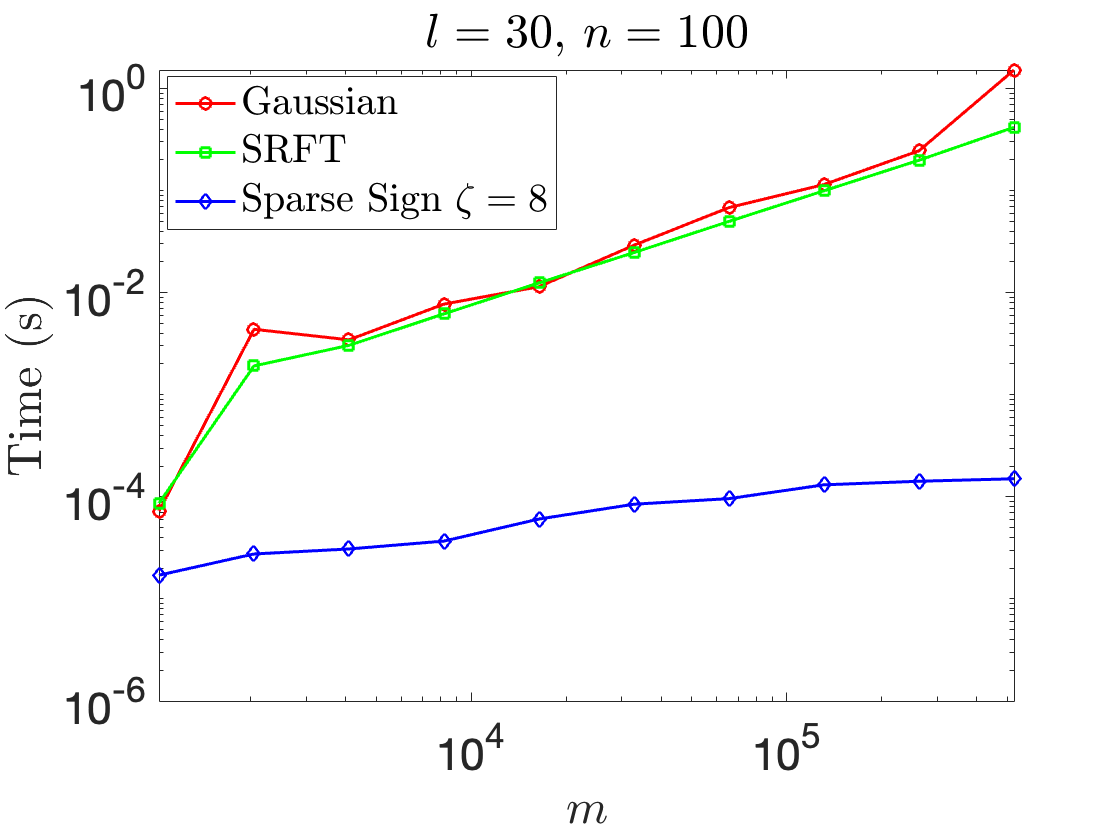
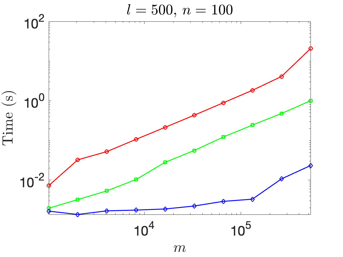
5.1. Computational speeds of different embeddings
Here, we compare the empirical efficiency of constructing sketches with some common randomized embeddings listed in Table 1. We consider applying an embedding of size to a matrix of size , which can be interpreted as embedding vectors in an ambient space to a lower dimensional space . We scale the experiments with respect to the ambient dimension , at several different embedding dimension , with a fixed number of repetitions . Figure 1 suggests that, with proper implementation, the sparse sign matrices are more efficient than the Gaussian embeddings and the SRTTs, especially for large scale problems. The SRTTs outperform Gaussian embeddings in terms of efficiency, and such advantage can be amplified as increases. These observations align with the asymptotic complexity in Table 1. While we also observe that, with MATLAB default implementation, the Gaussian embeddings usually enjoy matching efficiency as sparse sign matrices for moderate size problems, and are more efficient than SRTTs.
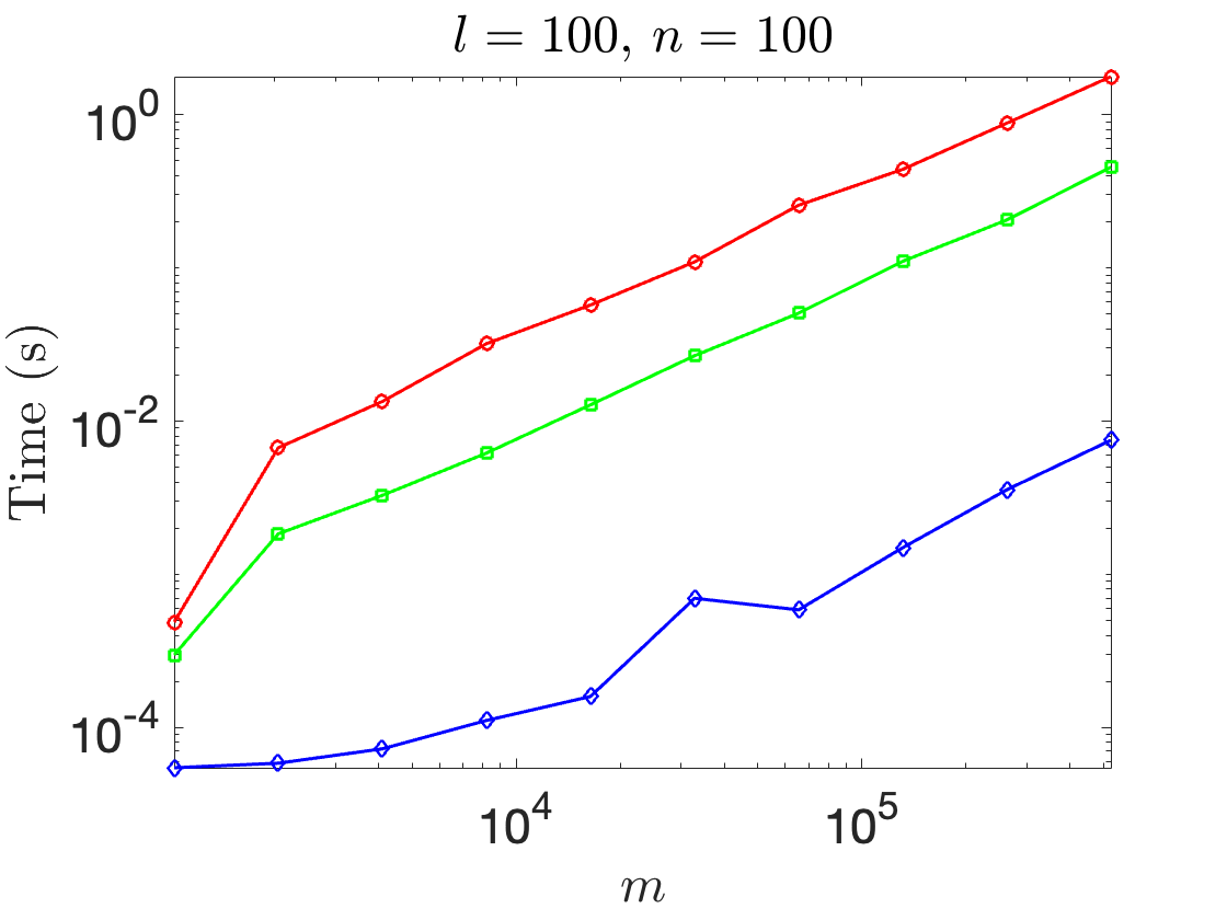
5.2. Computational speeds of different pivoting schemes
Given a sketch of , we isolate different pivoting schemes in Algorithm 1, and compare their run time as the problem size increases. Specifically, the LUPP and CPQR pivot directly on the given row sketch , while the DEIM involves one additional power iteration with orthogonalization (Section 2.4) before applying the LUPP (i.e., with a given column sketch , for DEIM, we first construct an orthonormal basis for columns of the sketch, and then we compute the reduced SVD for , and finally we column-wisely pivot on the resulting right singular vectors of size ).
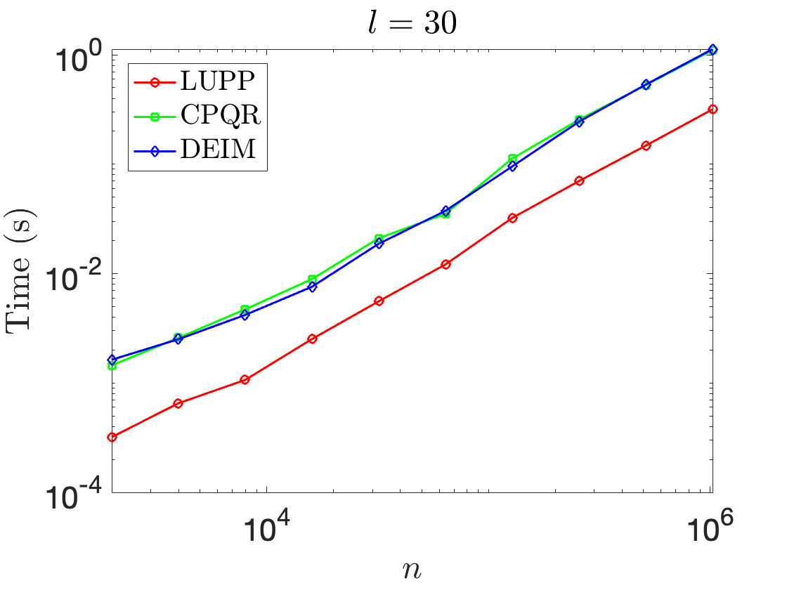
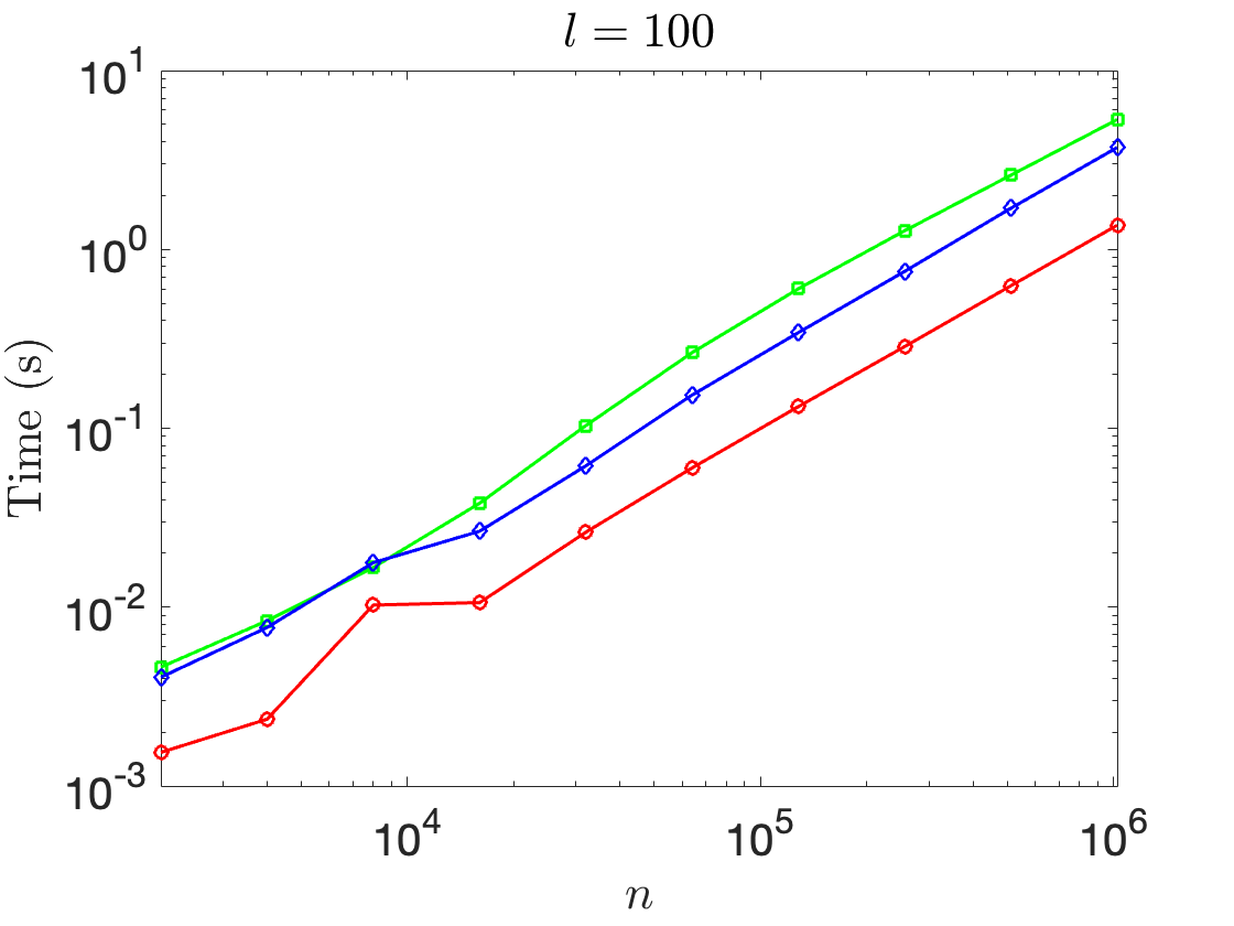
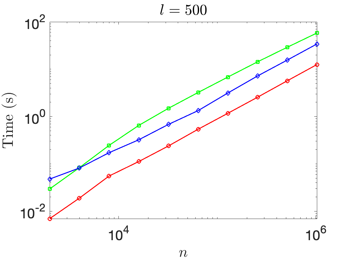
In Figure 2, we observe a considerable run time advantage of the LUPP over the CPQR and DEIM, especially when is large. (Additionally, we see that DEIM slightly outperforms CPQR, which is perhaps surprising, given the substantially larger number of flops required by DEIM.)
5.3. Randomized skeleton selection algorithms: accuracy and efficiency
As we move from measuring speed to measuring the precision of revealing the numerical rank of a matrix, the choice of test matrix becomes important. We consider four different classes of test matrices, including some synthetic random matrices with different spectral patterns, as well as some empirical datasets, as summarized below:
-
(1)
large: a full-rank sparse matrix with nonzero entries from the SuiteSparse matrix collection, generated by a linear programming problem sequence [40].
-
(2)
YaleFace64x64: a full-rank dense matrix, consisting of face images each of size . The flatten image vectors are centered and normalized such that the average image vector is zero, and the entries are bounded within .
-
(3)
MNIST training set consists of images of hand-written digits from to . Each image is of size . The images are flatten and normalized to form a full-rank matrix of size where is the number of images and is the size of the flatten images, with entries bounded in . The nonzero entries take approximately of the matrix for both the training and the testing sets.
-
(4)
Random sparse non-negative (SNN) matrices are synthetic random sparse matrices used in [58, 51] for testing skeleton selection algorithms. Given , a random SNN matrix of size takes the form,
(20) where , , are random sparse vectors with non-negative entries. In the experiments, we use two random SNN matrices of distinct sizes:
-
(i)
SNN1e3 is a SNN matrix with , for , and for ;
-
(ii)
SNN1e6 is a SNN matrix with , for , and for .
-
(i)
Scaled with respect to the approximation ranks , we compare the accuracy and efficiency of the following randomized CUR algorithms:
-
(1)
Rand-LUPP (and Rand-LUPP-1piter): Algorithm 1 with being a row sketch (or with one plain power iteration as in Equation 14), and pivoting with LUPP;
-
(2)
Rand-CPQR (and Rand-CPQR-1piter): Algorithm 1 with being a row sketch (or with one power iteration as in Equation 14), and pivoting with CPQR ([58]);
-
(3)
RSVD-DEIM: Algorithm 1 with being an approximation of leading- right singular vectors (Equation 16), and pivoting with LUPP ([51]);
-
(4)
RSVD-LS: Skeleton sampling based on approximated leverage scores ([37]) from a rank- SVD approximation (Equation 16);
-
(5)
SRCUR: Spectrum-revealing CUR decomposition proposed in [11].
The asymptotic complexities of the first three randomized pivoting based skeleton selection algorithms based on Algorithm 1 are summarized in Table 2.
| Algorithm | Row space approximator construction (Line 1,2) | Pivoting (Line 3) |
|---|---|---|
| Rand-LUPP | ||
| Rand-LUPP-1piter | ||
| Rand-CPQR | ||
| Rand-CPQR-1piter | ||
| RSVD-DEIM |
For consistency, we use Gaussian embeddings for sketching throughout the experiments. With the selected column and row skeletons, we leverage the stable construction in Equation 10 to form the corresponding CUR decompositions . Although oversampling (i.e., ) is necessary for multiplicative error bounds with respect to the optimal rank- approximation error (Equation 13, Theorem 1), since oversampling can be interpreted as a shift of curves along the axis of the approximation rank, for the comparison purpose, we simply treat , and compare the rank- approximation errors of the CUR decompositions against the optimal rank- approximation error .
From Figure 3-6, we observe that the randomized pivoting based skeleton selection algorithms that fall in Algorithm 1 (i.e., Rand-LUPP, Rand-CPQR, and RSVD-DEIM) share the similar approximation accuracy, which is considerably lower than the RSVD-LS and SRCUR. From the efficiency perspective, Rand-LUPP provides the most competitive run time among all the algorithms, especially when is sparse. Meanwhile, we observe that, for both Rand-CPQR and Rand-LUPP, constructing the sketches with one plain power iteration (i.e., with Equation 14) can observably improve the accuracy, without sacrificing the efficiency significantly (e.g., in comparison to the randomized DEIM which involves one power iteration with orthogonalization as in Section 2.4). In Figure 7, the similar performance is also observed on a synthetic large-scale problem, SNN1e6, where the matrix is only accessible as a fast matrix-vector multiplication (matvec) oracle such that each matvec takes (i.e., in our construction) operations.
Acknowledgments:
The work reported was supported by the Office of Naval Research (N00014-18-1-2354), by the National Science Foundation (DMS-1952735 and DMS-2012606), and by the Department of Energy ASCR (DE-SC0022251). The authors wish to thank Chao Chen, Ke Chen, Yuji Nakatsukasa, and Rachel Ward for valuable discussions.
References
- [1] Aizenbud, Y., Shabat, G., and Averbuch, A. Randomized lu decomposition using sparse projections. Computers & Mathematics with Applications 72, 9 (2016), 2525–2534.
- [2] Anderson, D., Du, S., Mahoney, M., Melgaard, C., Wu, K., and Gu, M. Spectral Gap Error Bounds for Improving CUR Matrix Decomposition and the Nyström Method. In Proceedings of the Eighteenth International Conference on Artificial Intelligence and Statistics (San Diego, California, USA, 09–12 May 2015), G. Lebanon and S. V. N. Vishwanathan, Eds., vol. 38 of Proceedings of Machine Learning Research, PMLR, pp. 19–27.
- [3] Anderson, D., and Gu, M. An efficient, sparsity-preserving, online algorithm for low-rank approximation. In Proceedings of the 34th International Conference on Machine Learning - Volume 70 (2017), ICML’17, JMLR.org, p. 156–165.
- [4] Batson, J. D., Spielman, D. A., and Srivastava, N. Twice-ramanujan sparsifiers. In Proceedings of the Forty-First Annual ACM Symposium on Theory of Computing (New York, NY, USA, 2009), STOC ’09, Association for Computing Machinery, p. 255–262.
- [5] Bebendorf, M. Approximation of boundary element matrices. Numerische Mathematik 86 (2000), 565–589.
- [6] Bien, J., Xu, Y., and Mahoney, M. Cur from a sparse optimization viewpoint. Annual Advances in Neural Information Processing Systems 24: Proceedings of the 2010 Conference (11 2010).
- [7] Boutsidis, C., Drineas, P., and Magdon-Ismail, M. Near optimal column-based matrix reconstruction. In 2011 IEEE 52nd Annual Symposium on Foundations of Computer Science (2011), pp. 305–314.
- [8] Boutsidis, C., and Gittens, A. Improved matrix algorithms via the subsampled randomized hadamard transform. SIAM Journal on Matrix Analysis and Applications 34, 3 (2013), 1301–1340.
- [9] Boutsidis, C., and Woodruff, D. P. Optimal cur matrix decompositions. In Proceedings of the Forty-Sixth Annual ACM Symposium on Theory of Computing (New York, NY, USA, 2014), STOC ’14, Association for Computing Machinery, p. 353–362.
- [10] Chan, T. F. Rank revealing qr factorizations. Linear Algebra and its Applications 88-89 (1987), 67–82.
- [11] Chen, C., Gu, M., Zhang, Z., Zhang, W., and Yu, Y. Efficient spectrum-revealing cur matrix decomposition. In Proceedings of the Twenty Third International Conference on Artificial Intelligence and Statistics (26–28 Aug 2020), S. Chiappa and R. Calandra, Eds., vol. 108 of Proceedings of Machine Learning Research, PMLR, pp. 766–775.
- [12] Clarkson, K. L., and Woodruff, D. P. Low-rank approximation and regression in input sparsity time. J. ACM 63, 6 (Jan. 2017).
- [13] Cohen, M. B., Lee, Y. T., Musco, C., Musco, C., Peng, R., and Sidford, A. Uniform sampling for matrix approximation. In Proceedings of the 2015 Conference on Innovations in Theoretical Computer Science (New York, NY, USA, 2015), ITCS ’15, Association for Computing Machinery, p. 181–190.
- [14] Cortinovis, A., and Kressner, D. Low-rank approximation in the frobenius norm by column and row subset selection, 2019.
- [15] Derezinski, M., Khanna, R., and Mahoney, M. W. Improved guarantees and a multiple-descent curve for the column subset selection problem and the nyström method. ArXiv abs/2002.09073 (2020).
- [16] Dereziński, M., and Mahoney, M. Determinantal point processes in randomized numerical linear algebra. Notices of the American Mathematical Society 68 (01 2021), 1.
- [17] Deshpande, A., and Rademacher, L. Efficient volume sampling for row/column subset selection. In 2010 IEEE 51st Annual Symposium on Foundations of Computer Science (2010), pp. 329–338.
- [18] Deshpande, A., Rademacher, L., Vempala, S., and Wang, G. Matrix approximation and projective clustering via volume sampling. Theory of Computing 2, 12 (2006), 225–247.
- [19] Drineas, P., Magdon-Ismail, M., Mahoney, M. W., and Woodruff, D. P. Fast approximation of matrix coherence and statistical leverage. J. Mach. Learn. Res. 13, 1 (Dec. 2012), 3475–3506.
- [20] Drineas, P., Mahoney, M. W., and Muthukrishnan, S. Relative-error $cur$ matrix decompositions. SIAM Journal on Matrix Analysis and Applications 30, 2 (2008), 844–881.
- [21] Drmač, Z., and Gugercin, S. A new selection operator for the discrete empirical interpolation method—improved a priori error bound and extensions. SIAM Journal on Scientific Computing 38, 2 (2016), A631–A648.
- [22] Eckart, C., and Young, G. The approximation of one matrix by another of lower rank. Psychometrika 1, 3 (Sep 1936), 211–218.
- [23] Geist, G. A., and Romine, C. H. $lu$ factorization algorithms on distributed-memory multiprocessor architectures. SIAM Journal on Scientific and Statistical Computing 9, 4 (1988), 639–649.
- [24] Golub, G. H., and Van Loan, C. F. Matrix Computations, third ed. The Johns Hopkins University Press, 1996.
- [25] Goreinov, S., Tyrtyshnikov, E., and Zamarashkin, N. A theory of pseudoskeleton approximations. Linear Algebra and its Applications 261, 1 (1997), 1–21.
- [26] Grigori, L., Demmel, J. W., and Xiang, H. Calu: A communication optimal lu factorization algorithm. SIAM Journal on Matrix Analysis and Applications 32, 4 (2011), 1317–1350.
- [27] Gu, M., and Eisenstat, S. C. Efficient algorithms for computing a strong rank-revealing qr factorization. SIAM Journal on Scientific Computing 17, 4 (1996), 848–869.
- [28] Halko, N., Martinsson, P. G., and Tropp, J. A. Finding structure with randomness: Probabilistic algorithms for constructing approximate matrix decompositions. SIAM Review 53, 2 (2011), 217–288.
- [29] Ho, K., Olver, S., Kelman, T., Jarlebring, E., TagBot, J., and Slevinsky, M. Lowrankapprox,jl: v0.4.3. https://github.com/JuliaMatrices/LowRankApprox.jl, 2020.
- [30] Hong, Y. P., and Pan, C.-T. Rank-revealing qr factorizations and the singular value decomposition. Mathematics of Computation 58, 197 (1992), 213–232.
- [31] Householder, A. S. Unitary triangularization of a nonsymmetric matrix. J. ACM 5, 4 (Oct. 1958), 339–342.
- [32] Indyk, P., and Motwani, R. Approximate nearest neighbors: Towards removing the curse of dimensionality. In Proceedings of the Thirtieth Annual ACM Symposium on Theory of Computing (New York, NY, USA, 1998), STOC ’98, Association for Computing Machinery, p. 604–613.
- [33] Kahan, W. Numerical linear algebra. Canadian Mathematical Bulletin 9, 5 (1966), 757–801.
- [34] Kezhong Zhao, Vouvakis, M. N., and Jin-Fa Lee. The adaptive cross approximation algorithm for accelerated method of moments computations of emc problems. IEEE Transactions on Electromagnetic Compatibility 47, 4 (2005), 763–773.
- [35] Kurzak, J., Luszczek, P., Faverge, M., and Dongarra, J. Lu factorization with partial pivoting for a multicore system with accelerators. IEEE Transactions on Parallel and Distributed Systems 24, 8 (2013), 1613–1621.
- [36] Liberty, E., Woolfe, F., Martinsson, P.-G., Rokhlin, V., and Tygert, M. Randomized algorithms for the low-rank approximation of matrices. Proceedings of the National Academy of Sciences 104, 51 (2007), 20167–20172.
- [37] Mahoney, M. W., and Drineas, P. Cur matrix decompositions for improved data analysis. Proceedings of the National Academy of Sciences 106, 3 (2009), 697–702.
- [38] Martinsson, P.-G., and Tropp, J. A. Randomized numerical linear algebra: Foundations and algorithms. Acta Numerica 29 (2020), 403–572.
- [39] Meng, X., and Mahoney, M. W. Low-distortion subspace embeddings in input-sparsity time and applications to robust linear regression. In Proceedings of the Forty-Fifth Annual ACM Symposium on Theory of Computing (New York, NY, USA, 2013), STOC ’13, Association for Computing Machinery, p. 91–100.
- [40] Meszaros, C. Meszaros/large, lp sequence: large000 to large036. http://old.sztaki.hu/~meszaros/public_ftp/lptestset/, 2004.
- [41] Miranian, L., and Gu, M. Strong rank revealing lu factorizations. Linear Algebra and its Applications 367 (07 2003), 1–16.
- [42] Musco, C., and Musco, C. Randomized block krylov methods for stronger and faster approximate singular value decomposition. In Proceedings of the 28th International Conference on Neural Information Processing Systems - Volume 1 (Cambridge, MA, USA, 2015), NIPS’15, MIT Press, p. 1396–1404.
- [43] Nelson, J., and Nguyên, H. L. Osnap: Faster numerical linear algebra algorithms via sparser subspace embeddings. In 2013 IEEE 54th Annual Symposium on Foundations of Computer Science (2013), pp. 117–126.
- [44] Pan, C.-T. On the existence and computation of rank-revealing lu factorizations. Linear Algebra and its Applications 316, 1 (2000), 199–222. Special Issue: Conference celebrating the 60th birthday of Robert J. Plemmons.
- [45] Pan, V. Y., Qian, G., and Yan, X. Random multipliers numerically stabilize gaussian and block gaussian elimination: Proofs and an extension to low-rank approximation. Linear Algebra and its Applications 481 (2015), 202–234.
- [46] Pan, V. Y., and Zhao, L. Numerically safe gaussian elimination with no pivoting. Linear Algebra and its Applications 527 (2017), 349–383.
- [47] Peters, G., and Wilkinson, J. H. On the stability of gauss-jordan elimination with pivoting. Commun. ACM 18, 1 (Jan. 1975), 20–24.
- [48] Rokhlin, V., and Tygert, M. A fast randomized algorithm for overdetermined linear least-squares regression. Proceedings of the National Academy of Sciences 105, 36 (2008), 13212–13217.
- [49] Shabat, G., Shmueli, Y., Aizenbud, Y., and Averbuch, A. Randomized lu decomposition. Applied and Computational Harmonic Analysis 44, 2 (2018), 246–272.
- [50] Solomonik, E., and Demmel, J. Communication-optimal parallel 2.5d matrix multiplication and lu factorization algorithms. In Euro-Par 2011 Parallel Processing (Berlin, Heidelberg, 2011), E. Jeannot, R. Namyst, and J. Roman, Eds., Springer Berlin Heidelberg, pp. 90–109.
- [51] Sorensen, D. C., and Embree, M. A deim induced cur factorization. SIAM Journal on Scientific Computing 38, 3 (2016), A1454–A1482.
- [52] Trefethen, L. N., and Bau, D. Numerical Linear Algebra. SIAM, 1997.
- [53] Trefethen, L. N., and Schreiber, R. S. Average-case stability of gaussian elimination. SIAM Journal on Matrix Analysis and Applications 11, 3 (1990), 335–360.
- [54] Tropp, J. A. Improved analysis of the subsampled randomized hadamard transform. Advances in Adaptive Data Analysis 03, 01n02 (2011), 115–126.
- [55] Tropp, J. A., Yurtsever, A., Udell, M., and Cevher, V. Fixed-rank approximation of a positive-semidefinite matrix from streaming data. In Advances in Neural Information Processing Systems (2017), I. Guyon, U. V. Luxburg, S. Bengio, H. Wallach, R. Fergus, S. Vishwanathan, and R. Garnett, Eds., vol. 30, Curran Associates, Inc.
- [56] Tropp, J. A., Yurtsever, A., Udell, M., and Cevher, V. Streaming low-rank matrix approximation with an application to scientific simulation. SIAM Journal on Scientific Computing 41, 4 (2019), A2430–A2463.
- [57] Tyrtyshnikov, E. Incomplete cross approximation in the mosaic-skeleton method. Computing 64, 4 (Jun 2000), 367–380.
- [58] Voronin, S., and Martinsson, P.-G. Efficient algorithms for cur and interpolative matrix decompositions. Advances in Computational Mathematics 43, 3 (Jun 2017), 495–516.
- [59] Wang, S., and Zhang, Z. A scalable cur matrix decomposition algorithm: Lower time complexity and tighter bound. In Proceedings of the 25th International Conference on Neural Information Processing Systems - Volume 1 (Red Hook, NY, USA, 2012), NIPS’12, Curran Associates Inc., p. 647–655.
- [60] Woodruff, D. P. Sketching as a tool for numerical linear algebra. Found. Trends Theor. Comput. Sci. 10, 1–2 (Oct. 2014), 1–157.
- [61] Woolfe, F., Liberty, E., Rokhlin, V., and Tygert, M. A fast randomized algorithm for the approximation of matrices. Applied and Computational Harmonic Analysis 25, 3 (2008), 335–366.
- [62] Çivril, A., and Magdon-Ismail, M. On selecting a maximum volume sub-matrix of a matrix and related problems. Theoretical Computer Science 410, 47 (2009), 4801–4811.