Improving repeatably in Matrix Factorization algorithms for Top-N recommendations

Improving stability in Matrix Factorization algorithms for Top-N recommendations

Improving stability in Matrix Factorization
for Top-N recommendations

On the instability of embedding-based recommenders: the case of Matrix Factorization

On the instability of embeddings for recommender systems:
the case of Matrix Factorization

Abstract.

Most state-of-the-art top-N collaborative recommender systems work by learning embeddings to jointly represent users and items. Learned embeddings are considered to be effective to solve a variety of tasks. Among others, providing and explaining recommendations. In this paper we question the reliability of the embeddings learned by Matrix Factorization (MF). We empirically demonstrate that, by simply changing the initial values assigned to the latent factors, the same MF method generates very different embeddings of items and users, and we highlight that this effect is stronger for less popular items. To overcome these drawbacks, we present a generalization of MF, called Nearest Neighbors Matrix Factorization (NNMF). The new method propagates the information about items and users to their neighbors, speeding up the training procedure and extending the amount of information that supports recommendations and representations. We describe the NNMF variants of three common MF approaches, and with extensive experiments on five different datasets we show that they strongly mitigate the instability issues of the original MF versions and they improve the accuracy of recommendations on the long-tail.

1. Introduction

The main goal of a wide variety of top-N collaborative recommender systems is to learn embeddings to jointly represent users and items (Cremonesi et al., 2010; He et al., 2017; Xue et al., 2017). Embeddings are derived in such a way that similar items (or similar users) have similar embeddings (Liang et al., 2016). Embeddings can be learnt with either Matrix Factorization (MF) or deep learning (DL) techniques (Koren et al., 2009; He et al., 2017). For both families of techniques, the learning procedure requires to sample the interaction space during the training (e.g., stochastic-gradient-descent (Ruder, 2016), skip-grams with negative sampling (Mikolov et al., 2013)).

Embedding-based models are characterized by various sources of randomness in their training, such as the initial values of the embeddings and the sampled interactions. Different random seeds or random generators might lead to different results in terms of embeddings learnt and, consequently, items recommended. The magnitude of these differences determines whether an algorithm can be considered stable or not. If these differences are too large (i.e, if the algorithm is not stable), we incur in severe issues that could mine the reliability and the credibility of a recommender. First, we cannot consider its recommendations to be reliable anymore, as the same algorithm executed on the same dataset could make totally different predictions for the same user-item pair (Madhyastha and Jain, 2019). Second, the instability of users’ and items’ representations may have strong implications in the explainability of the recommendations. Interpreting the predictions of embedding models is a difficult task, because there is not a clear and direct relationship between the representations learnt by the model and the attributes or the interactions of users and items. Most solutions provide explanations identifying similarities between the embeddings obtained by the model (Tintarev and Masthoff, 2007; Abdollahi and Nasraoui, 2017), but if the representations of users and items in the embedding space are not stable, the quality of such explanations might be compromised. Third, our definition of stability is strictly connected to that of repeatability as defined, for instance, in the SIGIR Initiative to implement the ACM Artifact Review and Badging guidelines. According to this definition, an unstable algorithm is not repeatable.

Alongside these examples, the works that leverage the embeddings of a model to various extents are not concerned with the potential consequences of this instability. Indeed, our notion of stability of a recommender system is different from what has been commonly addressed in the literature. Some works focus on the stability of the model when you introduce noisy or malicious perturbations in the dataset (Said et al., 2012; Mobasher et al., 2007), or when it evolves naturally with more interactions (Adomavicius and Zhang, 2014, 2012). In this work we focus on the stability of a recommender system when the same model is trained on the same dataset in exactly the same experimental conditions but with a different random sequence (e.g., due to a different random seed).

The variance in both the internal representation of the model (embeddings) and the output of the model (estimated relevance) can be reduced if enough samples are collected for each user and item to be modeled. Unfortunately, most datasets exhibit strong popularity biases (Anderson, 2006). Because of these biases, unpopular items (i.e., items with very few interactions) and short-profile users (i.e., users with very few interactions) will not collect enough samples during their training to smooth out the noise introduced by the randomness. Embeddings learnt on a small sample size will be biased and unstable (Skurichina and Duin, 1998).

Different techniques exist to improve the generalization capabilities of a model by leveraging or controlling the randomness of the training procedure. Bagging (Skurichina and Duin, 1998) is an ensemble method that trains different models from boostrap replica of the same dataset and average their predictions. However, it requires to retrain the model several times and is designed to improve the generalization capabilities and not to stabilize the model. Other techniques, such as Stochastic Weight Averaging (SWA), produce an ensemble by averaging the weights of the same model at different epochs of the training process (Madhyastha and Jain, 2019; Izmailov et al., 2018). In case of linear models, such as with Matrix Factorization, this is equivalent to averaging the embedding vectors during the gradient descent optimization. All these techniques are model agnostic and do not take into account the neighborhood properties of user and item embeddings: similar items (users) have similar embeddings.

In this paper, we focus on the stability of a widely employed family of embedding-based models, that is Matrix Factorization, as a function of random-seed. We are especially interested in investigating if MF based models under different initializations of latent factors generated by distinct random seeds, produce similar predictions and similar embeddings. We propose a new framework called Nearest Neighbors Matrix Factorization (NNMF), a generalization of classic Matrix Factorization that merges MF with nearest neighbors (NN) in order to alleviate the effects brought by the scarcity of interactions for unpopular items. While in classic MF the latent representations of items or users are treated independently, in NNMF we force each embedding to be a linear combination of the embeddings of a set of their most similar neighbors. With this approach we map the neighborhood relationships among items or users from the original interaction space to the new latent space. This mapping has the effect to propagate the updates applied to an item or a user also to their respective neighbors.

We provide an extensive set of experiments, testing NNMF with three MF approaches (BPR-MF, Funk-MF and P-MF) over five different datasets. The results show that:

• all the three MF methods suffer from the instability problem: on average, recommended items change by more than 50%;

• the three NNMF variants greatly improve stability: on average, recommended items change by less than 25%;

• the NNMF variants have better accuracy on the long tail with respect to the original MF methods, as well as other baselines, in almost all measures and datasets;

• the improved stability and the information propagation of NNMF allow to reach convergence in a fraction of the number of epochs required by MF.

The rest of the paper is organized as follows. In Section 2 we list a set of works related to the argument we treat in this paper. In Section 3 we introduce the issues of classic Matrix Factorization techniques and we present our new framework called Nearest Neighbor Matrix Factorization. We also describe some practical implementations over three well known MF algorithms. In Section 4 we discuss the results obtained by an extensive set of experiments over a variety of different datasets, testing the new models under different aspects. Finally, in Section 5, we provide some concluding remarks.

2. Related Work

There exist different definitions of stability of a recommender system in the literature, and different ways to improve each of these definitions. Most works define the stability of a recommender system as the ”consistent agreement of predictions” made to the same user by the same algorithm, when new incoming interactions are added to the system in complete agreement to system’s prior predictions (Adomavicius and Zhang, 2012). For instance, the work in (Adomavicius and Zhang, 2014) adopts bagging and iterative smoothing in conjunction with different traditional recommendation algorithms to improve their consistency. Other works define stability as the ability of the recommender system to provide consistent recommendations when malicious perturbations are performed to the dataset (Adomavicius and Zhang, 2012). The work in (Mobasher et al., 2007) suggests hybrid collaborative and content-based filtering as the best solution to mitigate the effects of attacks on the consistency of recommendations. Finally, other works (Said and Bellogín, 2018) relate the stability, or confidence, of a recommender system with the quality of a dataset, either at system level (the magic barrier described in (Said and Bellogín, 2018)) or at user-level (Bernardis et al., 2019). Our notion of stability – the consistency of both recommendations and latent representations of users and items when the same model is trained on exactly the same dataset with a different random sequence – is different from the definitions used in the literature.

There are also several works that try to control (or leverage) the randomness intrinsic in machine learning algorithms in order to improve the generalization capabilities of a model. Bagging is the most widely adopted black-box method used to leverage randomness in the input data in order improve the classification accuracy of a model (Skurichina and Duin, 1998). Bagging builds an ensemble of models by (i) running the same training algorithm on different boostrap replica of the same dataset and (ii) by aggregating their predictions. Training multiple model for prediction averaging, as with bagging, is computationally expensive. Therefore, other works train a single model and save the model parameters (snapshots) along the optimization path. The predictions of the snapshot models are later combined to produce the final prediction (Huang et al., 2017). Differently from bagging and snapshots, that build ensambles in the model space, other works build ensembles in the weights space. For instance, the works in (Madhyastha and Jain, 2019) and (Izmailov et al., 2018) use two variants of the same technique, Stochastic Weight Averaging (SWA), to compute a running average of the model weights during the last epochs of the training process.

Note also that even though the idea to merge MF and NN is not new (Nova et al., 2014; Koren, 2008), this is the first work, to the best of our knowledge, that addresses this particular stability issue and proposes a generic framework for MF that alleviates its drawbacks.

3. Models

In the following Sections, we denote with $\mathcal{U}$ and $\mathcal{I}$ the sets of users and items and with $|\mathcal{U}|$ and $|\mathcal{I}|$ their cardinalities. Lower case letters $u,v$ will be used to refer to users, while $i,j,k$ will refer to items. The user rating matrix (URM) is indicated by the uppercase bold letter $\mathbf{R}$ and each cell $r_{ui}$ contains the value of the preference, either explicit or implicit, if expressed, 0 otherwise. Lower case, bold letters indicate vectors in column format, unless differently specified. In particular, $\mathbf{r_{u}}$ indicates the user profile, intended as the $u$-th row of matrix $\mathbf{R}$. The set of $(u,i)$ couples for which $r_{ui}$ is known is denoted with $\kappa$.

In its basic form, MF consists in representing users and items in a latent factor space of dimension $f$. In particular, users and items are represented respectively in matrices $\mathbf{P}\in\mathbb{R}^{|\mathcal{U}|\times f}$ and $\mathbf{Q}\in\mathbb{R}^{|\mathcal{I}|\times f}$. A row $\mathbf{p_{u}}$ of $\mathbf{P}$ and $\mathbf{q_{i}}$ of $\mathbf{Q}$ handle, respectively, the representation of a user and an item on the same latent factor space. The dot product

(1) $$\overline{r}_{ui}=\mathbf{p_{u}}\text{\large{{\textperiodcentered}}}\mathbf{q_{i}^{T}}$$

measures how much user $u$ and item $i$ are aligned in the new latent space and therefore an estimate of the rating $\overline{r}_{ui}$ is provided. Consequently, the user-rating matrix can be estimated as:

(2) $$\overline{\mathbf{R}}=\mathbf{P}\mathbf{Q^{T}}$$

3.1. Matrix Factorization drawbacks

Over the years, researchers proposed various MF algorithms, varying how matrices $\mathbf{P}$ and $\mathbf{Q}$ are learned (Funk, 2006; Rendle et al., 2012; Salakhutdinov and Mnih, 2007) in order to improve the quality of recommendations under different aspects. Most of them learn the parameters of the model optimizing an objective function through stochastic gradient descent, iterating over the available data. The training phases of such algorithms share a common schema, which is partially altered from case to case. Firstly the two latent factor matrices $\mathbf{P}$ and $\mathbf{Q}$ are initialized with random values, then an iterative learning procedure begins. With each iteration, one or more interactions are selected among the available ones, and the objective function is computed alongside its respective gradient. Finally, the latent factors of the sampled items and users are updated accordingly.

The interactions are strongly biased towards popular items and long profiles. As such, the latent representations of users and items are updated based on this biased distribution: factors belonging to popular items (users) are updated far more often than niche ones. This means that the random initialization of the latent representations values for unpopular items and short-profile users has a strong impact on their final representations at convergence. We refer to this issue as instability of representations.

This problem directly affects also the recommendation lists generated by the algorithms: if the representation of a user is unstable, also the closest items in the latent space are unstable, leading to the generation of different recommendation lists for the same user, based on different random initial conditions. We refer to this issue as instability of recommendations.

Table 1. Stability of Top-10 recommendation lists generated by three MF techniques expressed with Jaccard index. Higher values indicate a better stability. Datasets names abbreviations are reported in Section 4.4.

Algorithm	LFM	M1M	BCR	PIN	CUL
BPR-MF	0.70	0.78	0.28	0.50	0.49
Funk-MF	0.72	0.60	0.05	0.28	0.31
P-MF	0.62	0.60	0.23	0.39	0.37

As an example, in Table 1 we show the stability of the top-10 recommendations for three common MF techniques, expressed with the Jaccard index, that indicates how much the generated lists overlap. The details of the experimental setup are described in Section 4. We compare the recommendations provided by 10 instances of the same model, all trained on the same data and with the same configuration, changing only the random seed, which, in turn, affects the initial values of the latent factors. The results in Table 1 show that, according to the Jaccard index, the recommendation lists overlap by less than 50% for three datasets out of five. For these datasets, more than 50% of the recommended items change by changing the initial random seed, i.e. by simply altering the initial values of the latent factors. For the BookCrossing dataset the instability is even more dramatic: lists overlap by less than 30%. More details about the experimental procedure and a wider range of experiments are described in Section 4.

3.2. Nearest Neighbors Matrix Factorization

The objective of MF is to learn users and items representations, also called embeddings, in a new latent space where users are mapped close to items they have expressed positive preference for. MF algorithms perform this task treating users and items as independent entities, without explicitly taking into account existing relationships among users and among items. However, these meaningful relationships should be reproduced also in the new latent space. We hence propose a new framework called Nearest Neighbors Matrix Factorization (NNMF), which is able to let Matrix Factorization algorithms leverage knowledge about users and items relationships, under the form of similarities, during the algorithm learning procedure. Given the two latent factor matrices $\mathbf{P}$ and $\mathbf{Q}$ defined in Section 3, we define the new neighborhood-aware latent representations for users $\mathbf{P^{*}}$ and items $\mathbf{Q^{*}}$

$$\mathbf{P^{*}}=\mathbf{S^{U}}\mathbf{P}\hskip 30.0pt\mathbf{Q^{*}}=\mathbf{S^{I}}\mathbf{Q}$$

where $\mathbf{S^{U}}$ and $\mathbf{S^{I}}$ are a user similarity matrix and an item similarity matrix, respectively, the first with size $|\mathcal{U}|\times|\mathcal{U}|$ and the second with size $|\mathcal{I}|\times|\mathcal{I}|$. Each element $s_{xy}$ stores the value of the similarity between entity $x$ and $y$, being them either users or items (i.e. $x,y\in\mathcal{U}$ or $x,y\in\mathcal{I}$). We require $s_{xx}$ to be equal to 1 for any $x$. Notice that if both similarity matrices $\mathbf{S^{U}}$ and $\mathbf{S^{I}}$ are identity matrices, NNMF collapses to classic MF. It follows that the new NNMF framework is a generalization of MF.

An important characteristic of the new technique can be highlighted by exploding the neighborhood-aware representations

(3) $$\mathbf{p^{*}_{u}}=\sum_{v\in\mathcal{U}}s^{U}_{uv}\mathbf{p_{v}}=\mathbf{p_{u}}+\sum_{v\in\mathcal{U}\setminus\{u\}}s^{U}_{uv}\mathbf{p_{v}}$$

(4) $$\mathbf{q^{*}_{i}}=\sum_{j\in\mathcal{I}}s^{I}_{ij}\mathbf{q_{j}}=\mathbf{q_{i}}+\sum_{j\in\mathcal{I}\setminus\{i\}}s^{I}_{ij}\mathbf{q_{j}}$$

We can clearly distinguish the contributions of the independent factors $\mathbf{p_{u}}$ and $\mathbf{q_{i}}$ from the contributions of the neighborhoods embeddings. The magnitude of the contribution of each neighbor is defined by the similarity with the user or the item we are considering: the more similar they are, the stronger the contribution will be. Finally, we can modify (2), used to estimate the preferences and provide recommendations, with the new formulation of the latent representations, rewriting it as:

(5) $$\overline{\mathbf{R}}=\mathbf{P^{*}}\mathbf{Q^{*T}}=\mathbf{S^{U}}\mathbf{P}\mathbf{Q^{T}}\mathbf{S^{I^{T}}}$$

(6) $$\overline{r}_{ui}=\mathbf{p^{*}_{u}}\text{\large{{\textperiodcentered}}}\mathbf{q^{*T}_{i}}=\bigg{(}\sum_{v\in U}s^{U}_{uv}\mathbf{p_{v}}\bigg{)}\text{\large{{\textperiodcentered}}}\bigg{(}\sum_{j\in I}s^{I}_{ij}\mathbf{q_{j}}\bigg{)}$$

In our implementation, the similarity matrices $\mathbf{S^{U}}$ and $\mathbf{S^{I}}$ are constant matrices that can be pre-computed by using any traditional nearest-neighbor collaborative-filtering approach. As such, NNMF can be easily applied to almost any MF algorithm.

Note that with the proposed formulation, $\mathbf{P}$ and $\mathbf{Q}$ do not directly contain users and items embeddings. They contain, instead, vectors that form a generating set, not necessarily a basis, for the vector space where users and items representations are projected. Embeddings for users and items are now contained in $\mathbf{P^{*}}$ and $\mathbf{Q^{*}}$, respectively. Another important aspect to notice is how an estimated rating $\overline{r}_{ui}$ is now dependent on multiple users and items and it is not restricted to $u$ and $i$ anymore.

There are two main advantages with NNMF over traditional MF. The first advantage is that it allows to have a larger amount of information supporting the latent representations of items and users, a particularly important aspect for users and items that have scarce data available, leading to a higher stability of recommendations and representations. The second advantage is that the updates made to the embeddings during the learning procedure are not restricted to the user and the item associated to the sampled interaction, but are also propagated to the representations of users and items in the neighborhoods of $u$ and $i$, resulting in a faster convergence of the model.

4. Experiments

4.1. Similarity

In the NNMF algorithm, relationships among users and items are modeled in the form of similarity matrices $\mathbf{S^{U}}$ and $\mathbf{S^{I}}$. Even though we did not make any assumption on how these matrices are obtained, for the experimental part of this paper we assume that the similarity values are calculated using the shrinked cosine similarity function:

(7) $$s_{uv}=\frac{\mathbf{r_{u}}\cdot\mathbf{r_{v}}}{||\mathbf{r_{u}}||\cdot||\mathbf{r_{v}}||+h_{U}}\hskip 56.9055pts_{ij}=\frac{\mathbf{r_{i}}\cdot\mathbf{r_{j}}}{||\mathbf{r_{i}}||\cdot||\mathbf{r_{j}}||+h_{I}}$$

where $\mathbf{r_{u}}$ and $\mathbf{r_{v}}$ are user profiles, $\mathbf{r_{i}}$ and $\mathbf{r_{j}}$ are item profiles and $h_{U}$ and $h_{I}$ are the shrink terms. Moreover, for every item and user we kept only a small number of the nearest neighbors, since we noticed that this approach led to the best performance.

Note that the choice of the cosine has two main advantages. The first is that it is simple and fast to compute. The second is that this way, the NNMF model has the same complexity of the original MF ones and also the same number of parameters to learn.

4.2. Instances

We experimented NNMF with three well known MF algorithms: Funk-MF (Funk, 2006), BPR-MF (Rendle et al., 2012) and P-MF (Salakhutdinov and Mnih, 2007).

• The NNMF loss function for Funk-MF is

  $$\sum_{(u,i)}\bigg{(}r_{ui}-\bigg{(}\sum_{v}s_{uv}\mathbf{p_{v}}\bigg{)}\text{\large{{\textperiodcentered}}}\bigg{(}\sum_{j}s_{ij}\mathbf{q_{j}}\bigg{)}\bigg{)}+\lambda_{p}\sum_{v}||\mathbf{p_{v}}||^{2}+\lambda_{q}\sum_{j}||\mathbf{q_{j}}||^{2}$$

  where $\lambda_{p}$ and $\lambda_{q}$ control the regularization.

• The maximum posterior estimator for the NNMF version of BPR-MF is

  $$\sum_{(u,i,j)}{\ln{\sigma(\overline{x}_{uij}(\Theta))}}+\lambda_{\Theta}\left\|\Theta\right\|^{2}$$

  where $\lambda_{\Theta}$ are model specific regularization parameters and $\sigma(\cdot)$ is the logistic function. The difference to the original MF version is in how $\overline{x}_{uij}(\Theta)$ is calculated, that for NNMF is

  $$\overline{x}_{uij}(\Theta)=\bigg{(}\sum_{v}s_{uv}\mathbf{p_{v}}\bigg{)}\text{\large{{\textperiodcentered}}}\bigg{(}\sum_{k}s_{ik}\mathbf{q_{k}}\bigg{)}-\bigg{(}\sum_{v}s_{uv}\mathbf{p_{v}}\bigg{)}\text{\large{{\textperiodcentered}}}\bigg{(}\sum_{k}s_{jk}\mathbf{q_{k}}\bigg{)}$$

• The loss of the NNMF version of P-MF is

  (8) $$\sum_{u,i}\bigg{(}r_{ui}-\sigma\bigg{(}\sum_{v}s_{uv}\mathbf{p_{v}}\text{\large{{\textperiodcentered}}}\sum_{k}s_{ik}\mathbf{q_{k}}\bigg{)}\bigg{)}^{2}+\frac{\lambda_{p}}{2}\sum_{u}||\mathbf{p_{u}}||^{2}+\frac{\lambda_{q}}{2}\sum_{i}||\mathbf{q_{i}}||^{2}$$

  where $\lambda_{p}$ and $\lambda_{q}$ are the regularization parameters.

In the experiments we forced all the NNMF models to use at least 2 neighbors for users or items, in order to ensure that a difference exists between the MF and the NNMF instances of the same approach. All the algorithms have been trained using an early stopping technique based on the accuracy performance on the validation set. We also performed a Bayesian optimization on a validation set to find the best parameters for every approach we tested. The source code used to perform the experiments is publicly available.

4.3. Baselines

We compare the stability of the NNMF algorithms with the stability of the corresponding standard MF algorithm. Moreover, we compare accuracy with some additional collaborative filtering baselines:

ItemKNN, UserKNN:

Traditional item and user-based nearest neighbors approaches with cosine similarity. (Ricci et al., 2010)

SLIM:

Linear regression model for top-n recommendation tasks with Bayesian Personalized Ranking as optimization function. (Ning and Karypis, 2011)

PureSVD:

Basic Matrix Factorization model based on SVD decomposition (Cremonesi et al., 2010). Notice that contrarily to the other MF methods we consider in this paper, it has an exact mathematical solution that can not include the similarity matrices introduced by NNMF.

All baselines have been tuned on a validation set by using a Bayesian optimizer.

4.4. Datasets

We carry out experiments employing a number of research datasets:

LastFM (LFM):

Implicit interactions gathered from the music website Last.fm. In particular, user listened artist relations expressed as listening counts. (Cantador et al., 2011)

Movielens1M (M1M):

Explicit interactions gathered from the website MovieLens. In particular, user rated movie relations. (Harper and Konstan, 2015)

BookCrossing (BCR):

Explicit interactions gathered from the online book club BookCrossing. In particular, user rated book relations. (Ziegler et al., 2005)

Pinterest (PIN):

Implicit interactions gathered from the social network Pinterest. In particular, user pin-to-own-board image relations. (Geng et al., 2015)

CiteULike (CUL):

Implicit interactions gathered from the online scientific community CiteULike. In particular, user saved-to-own-library paper relations. (Wang et al., 2013)

We employ datasets with densities of interactions that range from 0.04% to 2.51%, as we want to take into account the effect of a varying density of the datasets on both the accuracy and stability of the models. The statistical details of the datasets are described in Table 2.

Table 2. Statistics of the evaluation datasets

Dataset	Users	Items	Interactions	Density
LFM	1859	2823	42798	0.81%
M1M	6038	3307	501114	2.51%
BCR	13975	33925	314499	0.06%
PIN	55186	9637	877796	0.16%
CUL	5536	15429	119919	0.14%

The datasets used for the experiments have been preprocessed in two steps. First, we brought all the interactions to either zero or one by means of thresholding, since BPR requires binary preference values. Among the implicit datasets, only LFM needs thresholding: we use threshold value equal to one, hence we convert every interaction to one if the user has listened at least once to an artist. In explicit datasets we use threshold value equal to six for one to ten ratings and equal to three for one to five ratings. Second we applied a filtering procedure keeping only users and items with at least five interactions, in order to remove entities with a too scarce amount of information.

Each dataset has been randomly partitioned performing a standard holdout procedure in three sets: train, validation and test accounting for 60, 20 and 20 percent of the available interactions.

4.5. Stability of representations

Table 3. Stability of representations @10 expressed as Jaccard index. Underline indicates the most stable algorithm. Bold indicates which is more stable between MF and NNMF.

Algorithm	LFM		M1M		BCR		PIN		CUL
	Item	User	Item	User	Item	User	Item	User	Item	User
BPR-MF	0.73	0.67	0.70	0.70	0.47	0.32	0.45	0.30	0.57	0.58
BPR-NNMF	0.82	0.87	0.93	0.91	0.55	0.57	0.66	0.51	0.69	0.69
Funk-MF	0.66	0.61	0.36	0.33	0.17	0.13	0.34	0.19	0.48	0.48
Funk-NNMF	0.81	0.83	0.95	0.92	0.42	0.25	0.68	0.58	0.64	0.61
P-MF	0.62	0.56	0.55	0.47	0.38	0.26	0.32	0.19	0.60	0.40
P-NNMF	0.76	0.78	0.81	0.68	0.57	0.62	0.63	0.46	0.75	0.71

Assessing the stability of representations requires to use a technique which is invariant to transformations on the vector space, such as permutation or rotation of coordinates. The representation of an item, or user, is stable if, in every new latent space, it is close to the same items, or users. So we want to assess if the relationships among items and among users are maintained in the different embedding spaces and we can check this condition by ensuring that the neighborhoods formed in the new spaces are composed by the same set of users or items. Note that the cross-entity relationships between users and items are checked with the stability of recommendations experiment in the next section.

We compare MF and NNMF in a pairwise manner considering the differences in the stability of representations. Every algorithm tested is executed ten times, changing the latent factor initialization, an effect obtained simply using different seeds for the random number generator used to assign the initial values. The order in which the training data samples are explored during the different runs of the algorithms, instead, is ensured to be constant. We consider the latent factors representations learned and we create a list of the closest items to every item and users to every user, by means of a cosine similarity on the latent factor space. We compute these lists of $K$ nearest neighbors for the first of the ten models, both for MF and NNMF approaches. Then, we measure the degree of similarity of the $K$ nearest neighbors of the other nine models against the first considering the Jaccard index, a common statistic used to asses the similarity between sets. Higher similarity of the nearest neighbors in the latent space across different runs suggests a higher similarity of the latent factor representations. We performed the experiments using both $K=10$ and $K=100$ obtaining the same results, so, for brevity, in Table 3 we report only the results with $K=10$.

The most evident trend is that we have a large improvement in the stability of the recommendations when applying the new NNMF method with respect to original MF algorithm in every configuration. NNMF stability is over 50% in almost all the experiments, and well above 80% in two out of five datasets. MF approaches, on the contrary, struggle to reach 50% of stability for both users and items in three datasets out of five. Analyzing the results, we observe higher stability for denser datasets, while it drops when the density of interactions is really low. Among the MF algorithms, it is interesting to notice that the BPR-MF approach (and its NNMF variant) have a better stability than the other methods on almost all the experiments.

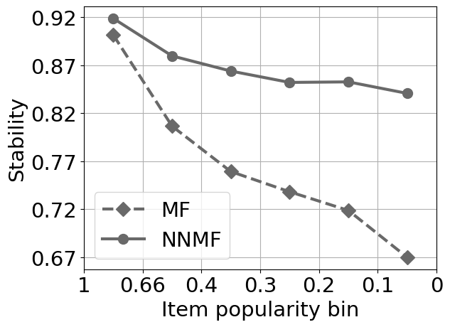
(a) BPR-MF vs BPR-NNMF

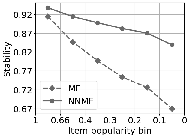
(b) Funk-MF vs Funk-NNMF

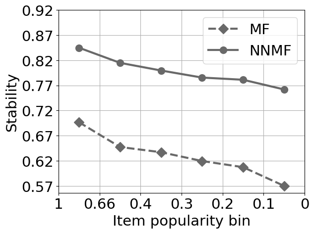
(c) P-MF vs P-NNMF

Figure 1. Stability of items representations for popularity ranges on the LFM dataset expressed as Jaccard @10. Every point represents the average stability value of the items in a bin. A bin contains all the items that belong to a range of popularity.

As second step of this experiment, we also want to understand if a correlation between the popularity of an item and its stability exists, so we analyze the items’ stabilities grouped by their popularity. We divide the items in 6 bins, depending on their popularity, using 1, 0.66, 0.4, 0.3, 0.2, 0.1 and 0 as thresholds. The first bin contains all the most popular items that account for the $1-0.66=34\%$ of the interactions in the dataset, i.e. the short-head. The second bin contains all the most popular items, excluding those in the first bin, that account for the $0.66-0.4=26\%$ of interactions. And so on. For each bin, we average the stability of the items that belong to it.

For brevity, in Figure 1 we show the results of the experiment performed only on the LFM dataset, but we obtained very similar results on all the datasets. As expected, the stability of NNMF models is globally higher than the MF counterparts. However, the plots show another clear trend: the representations of popular items are much more stable than unpopular ones. This behavior is not surprising, since higher popularity determines a higher number of updates and, consequently, a more detailed representation supported by a higher amount of information. Instead, niche items representations are subject of few updates during the learning process, resulting in more fuzzy representations even at model convergence, where the impact of the initialization values used is still strong. It is also evident that MF is subject to higher drops of stability, compared to NNMF, when passing from popular to niche items, widening the difference between them. The proposed analysis proves that the recommendations made by MF models are noisy and strongly impacted the random initialization of the latent factors, since the available information about the real user’s taste is often poor and marginally exploited. NNMF models, instead, are overall more stable, and the stability is high also when considering non-popular items. This has an impact also on the stability of recommendations and on the overall accuracy of the models, as we show in the following Sections.

4.6. Stability of recommendations

Table 4. Stability of recommendations @10 expressed as Jaccard index. Underline indicates the most stable algorithm. Bold indicates which is more stable between MF and NNMF.

Algorithm	LFM	M1M	BCR	PIN	CUL
BPR-MF	0.70	0.78	0.28	0.50	0.49
BPR-NNMF	0.86	0.95	0.52	0.69	0.65
Funk-MF	0.72	0.60	0.05	0.28	0.31
Funk-NNMF	0.87	0.95	0.18	0.75	0.51
P-MF	0.62	0.60	0.23	0.39	0.37
P-NNMF	0.79	0.76	0.61	0.78	0.66

As second experiment, we compare MF and NNMF in order to assess the differences in the stability of recommendations. The experimental procedure is similar to the one described in last Section: every algorithm tested is executed ten times, changing the latent factor initialization. But in this case we consider the top-10 recommendations provided by the ten models, both for MF and NNMF approaches, measuring the degree of similarity of the recommendations of the first model against the other nine, resorting again to the Jaccard index. Table 4 shows compatible results in the stability of recommendations with respect to what we observed for the representations in Table 3. The recommendation lists generated by NNMF models are always widely more stable than their MF counterparts. The MF implementations fail to reach the 50% threshold for the Jaccard index in many configurations, with a negative spike of 5% of Funk-MF on BCR. The NNMF versions largely mitigate this issue, as they are always able to outperform the respective MF implementations with a wide margin. As for the representations, also in this case the difference between dense datasets and sparse ones is evident, with a higher stability in the first scenario. Moreover, notice how the stability in both experiments tends to be higher for small datasets. This is not only related to the density of the dataset, since the number of items and users influence it, but having fewer items to take into account also reduces the different available options in the recommendation phase. As final observation, among the MF algorithms note that the BPR-MF approach is steadily better than the others on all the datasets, while among the NNMF this trend is not evident anymore.

4.7. Accuracy

Table 5. Long-tail accuracy. Bold indicates the best between MF and NNMF. Underline indicates the best performing algorithm.

Algorithm	LFM				M1M				BCR				PIN				CUL
	MAP		Recall		MAP		Recall		MAP		Recall		MAP		Recall		MAP		Recall
	@5	@10	@5	@10	@5	@10	@5	@10	@5	@10	@5	@10	@5	@10	@5	@10	@5	@10	@5	@10
ItemKNNCF	0.028	0.030	0.040	0.073	0.005	0.005	0.006	0.013	0.014	0.014	0.018	0.027	0.013	0.016	0.023	0.044	0.047	0.051	0.065	0.110
UserKNNCF	0.020	0.022	0.032	0.065	0.005	0.006	0.007	0.022	0.007	0.007	0.010	0.016	0.010	0.013	0.019	0.037	0.047	0.052	0.071	0.116
SLIM BPR	0.024	0.026	0.038	0.068	0.002	0.003	0.003	0.010	0.004	0.005	0.006	0.010	0.010	0.012	0.017	0.035	0.045	0.050	0.071	0.114
PureSVD	0.027	0.028	0.045	0.084	0.022	0.021	0.020	0.047	0.002	0.002	0.003	0.004	0.005	0.007	0.010	0.022	0.018	0.019	0.022	0.046
BPRMF	0.035	0.037	0.050	0.087	0.022	0.022	0.025	0.051	0.006	0.007	0.009	0.014	0.010	0.012	0.018	0.035	0.037	0.042	0.060	0.099
BPR NNMF	0.039	0.040	0.058	0.099	0.017	0.016	0.018	0.039	0.009	0.008	0.011	0.016	0.012	0.015	0.023	0.046	0.039	0.043	0.060	0.099
FunkSVD	0.033	0.035	0.050	0.085	0.017	0.015	0.018	0.034	0.004	0.004	0.006	0.009	0.010	0.013	0.019	0.037	0.044	0.049	0.069	0.108
Funk NNMF	0.033	0.036	0.052	0.094	0.034	0.028	0.024	0.046	0.006	0.007	0.010	0.016	0.011	0.014	0.021	0.041	0.053	0.058	0.080	0.127
ProbMF	0.019	0.020	0.030	0.058	0.008	0.009	0.010	0.027	0.001	0.001	0.002	0.003	0.009	0.011	0.016	0.033	0.033	0.038	0.052	0.090
Prob NNMF	0.034	0.036	0.054	0.095	0.027	0.024	0.025	0.048	0.007	0.007	0.009	0.014	0.011	0.013	0.020	0.038	0.047	0.049	0.064	0.107

Recommending non-popular items adds novelty and serendipity to the users, but it is usually a more difficult task compared to the recommendation of popular ones (Cremonesi et al., 2010). In this experiment we measure the accuracy of MF and NNMF in suggesting non-trivial items with a standard long-tail accuracy experiment, i.e. we compute the top-n performance of the algorithms using as ground truth the long-tail of the test set, while the training set is considered at its whole. We define as long-tail all the least popular items that account for the 66% of the interactions in the dataset. We evaluate the behavior of NNMF and MF approaches in this scenario, carrying out pairwise comparisons. Moreover, to provide context to our results, we additionally score other competitive collaborative baselines (Ferrari Dacrema et al., 2019) described in Section 4.3. In Table 5 we report the performance obtained by the different algorithms, expressed by the Mean Average Precision and the Recall at two cutoffs, 5 and 10. In almost 90% of the measures, the NNMF algorithms perform better than or equal to the corresponding MF versions, and in more than 80% of the measures, the improvement provided by NNMF is consistent.

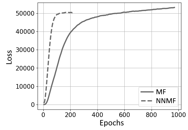
(a) BPR-Opt

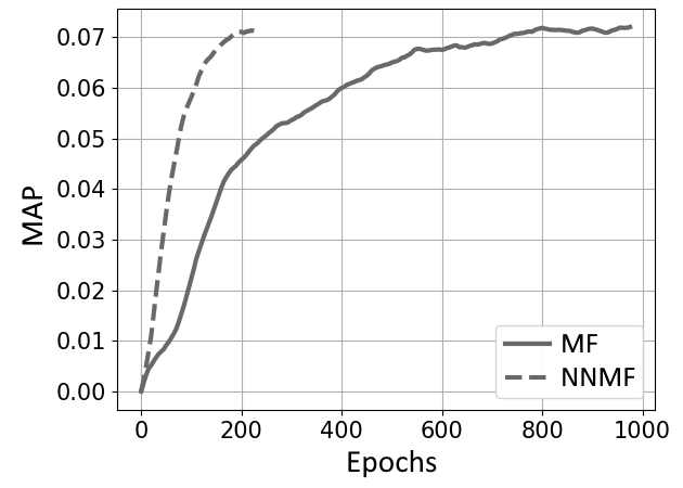
(b) MAP

Figure 2. Comparison between the training procedures of BPR-MF and BPR-NNMF on the CUL dataset. The plot on the left represents the BPR-Opt value on the training set. The plot on the right represents the MAP@5 obtained on the validation set.

NNMF models achieve highest accuracy on three datasets over five and in the remaining cases they try to fill the gap between the best performing model (usually ItemKNN) and classic MF algorithms, proving to be at least competitive against the other models across the datasets. Indeed, notice that even when a NNMF model is not the most accurate model on the long tail, it is the second best performing algorithm. The poor long-tail accuracy of MF obtained in many scenarios is quite surprising, especially if we consider that MF approaches are known for being less popularity biased than other CF approaches (Abdollahpouri et al., 2019; Channamsetty and Ekstrand, 2017; Jannach et al., 2013). We can conclude that these models are able to recommend niche items, but they are often noisy recommendations, resulting from the low number of updates on the latent factors of non-popular items, rather than a real evidence of the user’s taste. NNMF models, instead, leverage the knowledge of the neighborhood to construct more consistent item representations on the long-tail, transforming its part of non-popular recommendations in higher quality long-tail accuracy.

4.8. Model training

As last experiment, we also investigated the behavior of the models during the training procedure. For brevity, in Figure 2 we show, as an example, the comparison between BPR-MF and BPR-NNMF on the CUL dataset, but we could observe the same trend in all the other configurations. The plot on the left shows the maximum posterior estimator, called BPR-Opt in (Rendle et al., 2012), on the training set, while the one on the right shows the performance on the validation set, expressed as the MAP@5. Even if the starting and the convergence values of both the BPR-Opt and the MAP are quite similar between the two models, the NNMF version of the algorithm reaches lower BPR-Opt values and higher performance in a largely smaller amount of epochs. Indeed, notice that the NNMF version reaches convergence after about 200 epochs and the training is interrupted by the early stopping technique, while the original MF version needs about 1000 epochs to reach the same performance. This result proves that the propagation of the information we have about a user or an item also to its neighbors is very effective and useful, allowing the model to reach the optimal performance in a lower number of iterations over the training data.

5. Conclusions and Future Works

In this paper we present Nearest Neighbors Matrix Factorization, a generalization of classic Matrix Factorization. The new framework merges nearest neighbors and Matrix Factorization techniques in order to mitigate the drawbacks induced by the scarcity of collaborative information available, especially for unpopular items.

The results of extensive experiments on five different datasets show that classic MF approaches are particularly affected by instability. By simply changing the initial values assigned to the latent factors of users and items, the same model, trained on the same data and with the exactly same configuration, provides very different recommendations and latent representations of users and items at convergence, two issues that we call, respectively, instability of recommendations and instability of representations. Moreover, we show that exists a correlation between the popularity of an item and the stability of its representation.

To assess the validity of the new technique, we propose the NNMF extensions of three of the most common MF algorithms, checking the accuracy and the stability of the new models. The NNMF approaches provide large and consistent stability improvements in every scenario, and they are also able to increase the accuracy of their MF counterparts in almost every configuration, certifying the quality of the proposed framework. Finally, we show that the new models are able to reach convergence in a fraction of the epochs necessary to the MF approaches, thanks to the propagation of the information through the neighborhood relations.

Future works are addressed towards the study of the stability of more complex embedding-based models.

References

- (1)
- Abdollahi and Nasraoui (2017) Behnoush Abdollahi and Olfa Nasraoui. 2017. Using explainability for constrained matrix factorization. In Proceedings of the Eleventh ACM Conference on Recommender Systems. 79–83.
- Abdollahpouri et al. (2019) Himan Abdollahpouri, Masoud Mansoury, Robin Burke, and Bamshad Mobasher. 2019. The unfairness of popularity bias in recommendation. arXiv preprint arXiv:1907.13286 (2019).
- Adomavicius and Zhang (2012) Gediminas Adomavicius and Jingjing Zhang. 2012. Stability of recommendation algorithms. ACM Transactions on Information Systems (TOIS) 30, 4 (2012), 1–31.
- Adomavicius and Zhang (2014) Gediminas Adomavicius and Jingjing Zhang. 2014. Improving stability of recommender systems: a meta-algorithmic approach. IEEE Transactions on Knowledge and Data Engineering 27, 6 (2014), 1573–1587.
- Anderson (2006) Chris Anderson. 2006. The long tail: Why the future of business is selling less of more. Hachette Books.
- Bernardis et al. (2019) Cesare Bernardis, Maurizio Ferrari Dacrema, and Paolo Cremonesi. 2019. Estimating Confidence of Individual User Predictions in Item-Based Recommender Systems. In Proceedings of the 27th ACM Conference on User Modeling, Adaptation and Personalization (UMAP ’19). Association for Computing Machinery, New York, NY, USA, 149–156. https://doi.org/10.1145/3320435.3320453
- Cantador et al. (2011) Iván Cantador, Peter Brusilovsky, and Tsvi Kuflik. 2011. Second workshop on information heterogeneity and fusion in recommender systems (HetRec2011). In Proceedings of the fifth ACM conference on Recommender systems. ACM, New York, NY, USA, 387–388.
- Channamsetty and Ekstrand (2017) Sushma Channamsetty and Michael D Ekstrand. 2017. Recommender response to diversity and popularity bias in user profiles. In The Thirtieth International Flairs Conference.
- Cremonesi et al. (2010) Paolo Cremonesi, Yehuda Koren, and Roberto Turrin. 2010. Performance of Recommender Algorithms on Top-n Recommendation Tasks. In Proceedings of the Fourth ACM Conference on Recommender Systems (RecSys ’10). Association for Computing Machinery, New York, NY, USA, 39–46. https://doi.org/10.1145/1864708.1864721
- Ferrari Dacrema et al. (2019) Maurizio Ferrari Dacrema, Paolo Cremonesi, and Dietmar Jannach. 2019. Are We Really Making Much Progress? A Worrying Analysis of Recent Neural Recommendation Approaches. https://doi.org/10.1145/3298689.3347058
- Funk (2006) Simon Funk. 2006. Netflix Update: Try This At Home. http://sifter.org/ simon/journal/20061211.html (2006).
- Geng et al. (2015) Xue Geng, Hanwang Zhang, Jingwen Bian, and Tat-Seng Chua. 2015. Learning image and user features for recommendation in social networks. In Proceedings of the IEEE International Conference on Computer Vision. 4274–4282.
- Harper and Konstan (2015) F. Maxwell Harper and Joseph A. Konstan. 2015. The MovieLens Datasets: History and Context. ACM Trans. Interact. Intell. Syst. 4, Article 19 (Dec. 2015), 19 pages. https://doi.org/10.1145/2827872
- He et al. (2017) Xiangnan He, Lizi Liao, Hanwang Zhang, Liqiang Nie, Xia Hu, and Tat-Seng Chua. 2017. Neural collaborative filtering. In Proceedings of the 26th international conference on world wide web. 173–182.
- Huang et al. (2017) Gao Huang, Yixuan Li, Geoff Pleiss, Zhuang Liu, John E Hopcroft, and Kilian Q Weinberger. 2017. Snapshot ensembles: Train 1, get m for free. arXiv preprint arXiv:1704.00109 (2017).
- Izmailov et al. (2018) Pavel Izmailov, Dmitrii Podoprikhin, Timur Garipov, Dmitry Vetrov, and Andrew Gordon Wilson. 2018. Averaging weights leads to wider optima and better generalization. arXiv preprint arXiv:1803.05407 (2018).
- Jannach et al. (2013) Dietmar Jannach, Lukas Lerche, Fatih Gedikli, and Geoffray Bonnin. 2013. What Recommenders Recommend – An Analysis of Accuracy, Popularity, and Sales Diversity Effects. In User Modeling, Adaptation, and Personalization, Sandra Carberry, Stephan Weibelzahl, Alessandro Micarelli, and Giovanni Semeraro (Eds.). Springer Berlin Heidelberg, Berlin, Heidelberg, 25–37.
- Koren (2008) Yehuda Koren. 2008. Factorization Meets the Neighborhood: A Multifaceted Collaborative Filtering Model (KDD ’08). Association for Computing Machinery, New York, NY, USA, 426–434. https://doi.org/10.1145/1401890.1401944
- Koren et al. (2009) Yehuda Koren, Robert Bell, and Chris Volinsky. 2009. Matrix factorization techniques for recommender systems. Computer 42, 8 (2009), 30–37.
- Liang et al. (2016) Dawen Liang, Jaan Altosaar, Laurent Charlin, and David M Blei. 2016. Factorization meets the item embedding: Regularizing matrix factorization with item co-occurrence. In Proceedings of the 10th ACM conference on recommender systems. 59–66.
- Madhyastha and Jain (2019) Pranava Madhyastha and Rishabh Jain. 2019. On Model Stability as a Function of Random Seed. arXiv preprint arXiv:1909.10447 (2019).
- Mikolov et al. (2013) Tomáš Mikolov, Wen-tau Yih, and Geoffrey Zweig. 2013. Linguistic regularities in continuous space word representations. In Proceedings of the 2013 conference of the north american chapter of the association for computational linguistics: Human language technologies. 746–751.
- Mobasher et al. (2007) Bamshad Mobasher, Robin Burke, Runa Bhaumik, and Jeff J Sandvig. 2007. Attacks and remedies in collaborative recommendation. IEEE Intelligent Systems 22, 3 (2007), 56–63.
- Ning and Karypis (2011) X. Ning and G. Karypis. 2011. SLIM: Sparse Linear Methods for Top-N Recommender Systems. In 2011 IEEE 11th International Conference on Data Mining. 497–506.
- Nova et al. (2014) David Nova, Pablo A. Estévez, and Pablo Huijse. 2014. K-Nearest Neighbor Nonnegative Matrix Factorization for Learning a Mixture of Local SOM Models. In Advances in Self-Organizing Maps and Learning Vector Quantization, Thomas Villmann, Frank-Michael Schleif, Marika Kaden, and Mandy Lange (Eds.). Springer International Publishing, Cham, 229–238.
- Rendle et al. (2012) Steffen Rendle, Christoph Freudenthaler, Zeno Gantner, and Lars Schmidt-Thieme. 2012. BPR: Bayesian Personalized Ranking from Implicit Feedback. CoRR abs/1205.2618 (2012). arXiv:1205.2618 http://arxiv.org/abs/1205.2618
- Ricci et al. (2010) Francesco Ricci, Lior Rokach, Bracha Shapira, and Paul B. Kantor. 2010. Recommender Systems Handbook (1st ed.). Springer-Verlag, Berlin, Heidelberg.
- Ruder (2016) Sebastian Ruder. 2016. An overview of gradient descent optimization algorithms. arXiv preprint arXiv:1609.04747 (2016).
- Said and Bellogín (2018) Alan Said and Alejandro Bellogín. 2018. Coherence and inconsistencies in rating behavior: estimating the magic barrier of recommender systems. User Modeling and User-Adapted Interaction 28, 2 (2018), 97–125.
- Said et al. (2012) Alan Said, Brijnesh J Jain, Sascha Narr, and Till Plumbaum. 2012. Users and noise: The magic barrier of recommender systems. In International Conference on User Modeling, Adaptation, and Personalization. Springer, 237–248.
- Salakhutdinov and Mnih (2007) Ruslan Salakhutdinov and Andriy Mnih. 2007. Probabilistic Matrix Factorization. In Proceedings of the 20th International Conference on Neural Information Processing Systems (NIPS ’07). Curran Associates Inc., USA, 1257–1264. http://dl.acm.org/citation.cfm?id=2981562.2981720
- Skurichina and Duin (1998) Marina Skurichina and Robert PW Duin. 1998. Bagging for linear classifiers. Pattern Recognition 31, 7 (1998), 909–930.
- Tintarev and Masthoff (2007) Nava Tintarev and Judith Masthoff. 2007. A survey of explanations in recommender systems. In 2007 IEEE 23rd international conference on data engineering workshop. IEEE, 801–810.
- Wang et al. (2013) Hao Wang, Binyi Chen, and Wu-Jun Li. 2013. Collaborative Topic Regression with Social Regularization for Tag Recommendation. In IJCAI.
- Xue et al. (2017) Hong-Jian Xue, Xinyu Dai, Jianbing Zhang, Shujian Huang, and Jiajun Chen. 2017. Deep Matrix Factorization Models for Recommender Systems.. In IJCAI. 3203–3209.
- Ziegler et al. (2005) Cai-Nicolas Ziegler, Sean M. McNee, Joseph A. Konstan, and Georg Lausen. 2005. Improving Recommendation Lists through Topic Diversification. In Proceedings of the 14th International Conference on World Wide Web (WWW ’05). Association for Computing Machinery, New York, NY, USA, 22–32. https://doi.org/10.1145/1060745.1060754