Efficient algorithms for computing a rank-revealing UTV factorization on parallel computing architectures
Abstract
The randomized singular value decomposition (RSVD) is by now a well established technique for efficiently computing an approximate singular value decomposition of a matrix. Building on the ideas that underpin the RSVD, the recently proposed algorithm “randUTV” computes a full factorization of a given matrix that provides low-rank approximations with near-optimal error. Because the bulk of randUTV is cast in terms of communication-efficient operations like matrix-matrix multiplication and unpivoted QR factorizations, it is faster than competing rank-revealing factorization methods like column pivoted QR in most high performance computational settings. In this article, optimized randUTV implementations are presented for both shared memory and distributed memory computing environments. For shared memory, randUTV is redesigned in terms of an algorithm-by-blocks that, together with a runtime task scheduler, eliminates bottlenecks from data synchronization points to achieve acceleration over the standard blocked algorithm, based on a purely fork-join approach. The distributed memory implementation is based on the ScaLAPACK library. The performances of our new codes compare favorably with competing factorizations available on both shared memory and distributed memory architectures.
1 Introduction.
1.1 Overview.
Computational linear algebra faces significant challenges as high performance computing moves further away from the serial into the parallel. Classical algorithms were designed to minimize the number of floating point operations, and do not always lead to optimal performance on modern communication-bound architectures. The obstacle is particularly apparent in the area of rank-revealing matrix factorizations. Traditional techniques based on column pivoted QR factorizations or Krylov methods tend to be challenging to parallelize well, as they are most naturally viewed as a sequence of matrix-vector operations.
In this paper, we describe techniques for efficiently implementing a randomized algorithm for computing a so-called rank-revealing UTV decomposition [21]. Given an input matrix of size , the objective is to compute a factorization
| (1) |
where the middle factor is upper triangular (or upper trapezoidal in the case ) and the left and right factors are orthogonal. The factorization is rank-revealing in the sense that
| (2) |
In a factorization resulting from randUTV, the middle matrix often has elements above the diagonal that are very small in modulus, which means that the diagonal entries of become excellent approximations to the singular values of . A factorization of this type is useful for solving tasks such as low-rank approximation, for determined basis to approximations to the fundamental subspaces of , for solving ill-conditioned or over/under-determined linear systems in a least-square sense, and for estimating the singular values of .
The randomized UTV algorithm randUTV that we implement has characteristics that in many environments make it preferable to classical rank-revealing factorizations like column pivoted QR (CPQR) and the singular value decomposition (SVD):
-
•
It consistently produces matrix factors which yield low-rank approximations with accuracy comparable to the SVD. The particular use of randomization in the algorithm is essentially risk free. The reliability of the method is supported by theoretical analysis, as well as extensive numerical experiments.
-
•
It casts most of its operations in terms of matrix-matrix multiplications, which are highly efficient in parallel computing environments. It was demonstrated in [21] that a straightforward blocked implementation of randUTV executes faster than even highly optimized implementations of CPQR in symmetric multiprocessing (SMP) systems. In this manuscript, we present an implementation that improves on the performances in [21] for SMP and obtain similar findings for distributed memory architectures.
-
•
It processes the input matrix in sets of multiple columns, so it can be stopped part way through the factorization process if it is found that a requested tolerance has been met. If columns end up having been computed, only flops will have been expended.
In this manuscript, we present two efficient implementations for computing the randUTV factorization: the first one for shared-memory machines, and the second one for distributed-memory machines. Regarding shared-memory architectures, the implementation presented in our paper [21] proposed a blocked algorithm in which parallelism was extracted on a per-task basis, relying on parallel BLAS implementations, and hence following a fork-join parallel execution model. Here, we propose a novel algorithm-by-blocks [28], in which sequential tasks are dynamically added to a Directed Acyclic Graph (DAG) and executed by means of a runtime task scheduler (libflame’s SuperMatrix [6]). This approach enhances performance by mitigating the effects of the inherent synchronization points in fork-join models, and has shown its potential in other linear algebra implementations [7]. In addition, given the recent improvements in terms of performance of modern SVD implementations (e.g. in Intel MKL), we show how runtime-based implementations of randUTV are still on par with them in terms of performance. Regarding our second proposal, it is the first time a distributed-memory version of randUTV is presented in the literature; performance results reveal excellent scalability results compared with state-of-the-art distributed-memory implementations.
Specifically, the main contributions of the paper compared with the state-of-the-art are:
-
1.
We propose a novel algorithm-by-blocks for computing the randUTV factorization that maximizes performance at no programmability cost.
-
2.
We have integrated our solution with an existing task-based software infrastructure (libflame SuperMatrix), hence providing an out-of-the-box implementation based on tasks for randUTV.
-
3.
On shared-memory architectures, we provide a detailed study of the optimal block sizes compared with a parallel-BLAS-based solution, and report qualitative and quantitative differences between them that can be of interest for the community. Similarly, we have carried out a detailed performance and scalability study on two highly-parallel shared-memory machines.
-
4.
Performance results reveal the benefits of the algorithm-by-blocks compared with the blocked algorithm on our target testbed, yielding performance improvements between and for the largest tested matrices. Accelerations compared with proprietary MKL SVD implementations also reveal substantial performance gains, with improvements up to for selected cases, and in general in all cases that involve relatively large matrices ().
-
5.
On distributed-memory architectures, the comparison in terms of execution time with ScaLAPACK SVD and CPQR and PLiC CPQR reveal consistent performance gains ranging from to , and an excellent scalability on the tested platforms.
-
6.
On distributed-memory architectures, we provide a detailed performance study regarding block sizes, grid sizes, threads per process, etc. on several number of nodes.
The paper is structured as follows: We first discuss the notation that will be used throughout the paper in Section 2. In Section 3, we familiarize the reader with the randUTV algorithm that was recently described in [21]. Sections 4 and 5 describe the shared and distributed memory implementations that form the main contribution of this manuscript. In Section 6, we present numerical results that compare our implementations to highly optimized implementations of competing factorizations. Section 7 summarizes the key findings and outlines some possibilities for further improvements and extensions.
2 Preliminaries.
We use the notation to specify that is an matrix with real entries. An orthogonal matrix is a square matrix whose column vectors each have unit norm and are pairwise orthogonal. represents the -th singular value of , and . The default norm is the spectral norm. We also use the standard matrix indexing notation to denote the submatrix of consisting of the entries in the -th through -th rows of the -th through -th columns.
2.1 The Singular Value Decomposition (SVD)
Let and . It is well known [15, 34, 33] that any matrix admits a singular value decomposition (SVD) of the form
where and are orthogonal and is diagonal. We may also speak of the economic SVD of , given by
in which case and are not necessarily orthogonal (because they are not square), but their columns remain orthonormal. The diagonal elements of are the singular values of . These are ordered so that . The columns and of and are called the left and right singular vectors, respectively, of .
A key fact about the SVD is that it provides theoretically optimal rank- approximations to . Specifically, the Eckart-Young-Mirsky Theorem [13, 25] states that given the SVD of a matrix as described above and a fixed , we have that
A corollary of this result is that the subspaces spanned by the leading left and right singular vectors of provide the optimal rank- approximations to the column and row spaces, respectively, of . For instance, if is the orthogonal projection onto the subspace spanned by the left singular vectors of , then , so .
2.2 The QR decomposition
Given a matrix , let . A QR decomposition of is given by
where is orthogonal and is upper triangular. If , then any QR can be reduced to the “economic” QR
The standard algorithm for computing a QR factorization relies on Householder reflectors. We refer to this algorithm as HQR in this article. A full discussion of the HQR algorithm can be found in [15, 34, 33]; for our purposes, it is only necessary to note that the outputs of HQR are the following: an upper triangular matrix of the QR factorization, and a unit lower triangular matrix and a vector that can be used to build or to apply (see Section 2.3). 555We should say that holds the “Householder vectors”. In this article, we make critical use of the fact that for , the leading columns of form an orthonormal basis for the column space of .
2.3 Compact representation of collections of Householder reflectors.
Consider a matrix , and let be Householder transformations. As a Householder transformation has the following structure: , applying it to a matrix requires a matrix-vector product and a rank-1 update. If all are applied one after another, the computation requires flops in overall because of the special structure of the Householder transformations. Both operations are matrix-vector based, and therefore they do not render high performances on modern architectures.
If several Householder transformations must be applied, the product may be expressed in the form
where is lower trapezoidal and is upper triangular. This formation of the product of Householder matrices is called the compact representation [30]. If the Householder transformations used to form each are known, matrices and of the compact are inexpensive to compute. The above expression can be used to build the product :
In this case, the cost is about the same, but only matrix-matrix operations are employed. Since on modern architectures matrix-matrix operations are usually much more efficient that matrix-vector operations, this approach will render higher performances. Recall that one flop (floating-point operation) in a matrix-matrix operation can be much faster (several times) than a flop in a matrix-vector operation.
3 The UTV factorization.
In this section, we discuss the rank-revealing UTV matrix factorization, establishing its usefulness in computational linear algebra and reviewing efficient algorithms for its computation. In Section 3.1, we review the classical UTV matrix decomposition, summarizing its benefits over other standard decompositions like column-pivoted QR and the SVD. In Section 3.2, we summarize recent work [21] that proposes a randomized blocked algorithm for computing this factorization.
3.1 The classical UTV factorization.
Let and set . A UTV decomposition of is any factorization of the form
| (3) |
where is triangular and and are both orthogonal. In this paper, we take to be upper triangular, which is typically the more convenient choice when . It is often desirable to compute a rank-revealing UTV (RRUTV) decomposition. For any , consider the partitioning of
| (4) |
where is . We say a UTV factorization is rank-revealing if
-
1.
,
-
2.
.
The flexibility of the factors in a UTV decomposition renders certain advantages over other canonical forms like CPQR and SVD (note that each of these are specific examples of UTV factorizations). Since the right factor in CPQR is restricted to a permutation matrix, UTV has more freedom to provide better low-rank and subspace approximations. Also, since UTV does not have the SVD’s restriction of diagonality on the middle factor, the UTV is less expensive to compute and has more efficient methods for updating and downdating (see, e.g. [31, 32, 2, 14, 26]).
3.2 The randUTV algorithm.
In [21], a new algorithm called randUTV was proposed for computing an RRUTV factorization. randUTV is designed to parallelize well, enhancing the RRUTVs viability as a competitor to both CPQR and the SVD for a wide class of problem types. It yields low-rank approximations comparable to the SVD at computational speeds that match, and in many cases outperform both CPQR and SVD. Unlike classical methods for building SVDs and RRUTVs, randUTV processes the input matrix by blocks of contiguous columns. randUTV shares the advantage of CPQR that the factorization is computed incrementally, and may be stopped early to incur an overall cost of , where is the rank of the computed factorization.
The driving idea behind the structure of the randUTV algorithm is to build the middle factor with a right-looking approach, that is, in each iteration multiple columns of (a column block) are obtained simultaneously and only the right part of is accessed. To illustrate, consider an input matrix , and let A block size parameter with must be chosen before randUTV begins. For simplicity, assume divides evenly. The algorithm begins by initializing . Then, the bulk of the work is done in a loop requiring steps. In the -th step, a new matrix is computed with
for some orthogonal matrices and . and are chosen such that:
-
•
the leading columns of are upper triangular with diagonal blocks on the main diagonal.
-
•
using the partitioning in Equation 4 to define and , we have and for .
-
•
for .
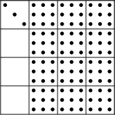
An example of the sparsity patterns for each is shown in Figure 1.
 |
 |
 |
| after 0 steps: | after 1 step: | after 2 steps: |
Once is upper triangular, and can then be built with
and
In practice, and are constructed in two separate stages and applied to at different points in the algorithm. We will henceforth refer to these matrices as and for the first and second stages, respectively. Also, just one matrix is stored, whose contents are overwritten with the new at each step. Similarly, in case the matrices and are required to be formed, only one matrix and one matrix would be stored. The outline for randUTV is therefore the following:
-
1.
Initialize .
-
2.
for :
-
i.
Build .
-
ii.
Update and : .
-
iii.
Build .
-
iv.
Update and : .
-
v.
Build and simultaneously.
-
vi.
Update , , and : , , .
-
i.
A matlab code for an easily readable (but inefficient) implementation of randUTV is given in Figure 2.
3.2.1 Building .
is constructed to maximize the rank-revealing properties of the final factorization. Specifically, consider the partitioning at step of matrices and
where the top left block of each partition is . Then is constructed such that the leading columns of form an orthonormal approximate basis for the leading right singular vectors of . An efficient method for such a construction has been developed recently (see, e.g. [29, 18, 24, 22, 23]) using ideas in random matrix theory. is built as follows:
-
1.
Draw a thin Gaussian random matrix .
-
2.
Compute for some small integer .
-
3.
Perform an unpivoted QR factorization on to obtain an orthogonal and upper triangular such that .
-
4.
Set .
The parameter , often called the “power iteration” parameter, determines the accuracy of the approximate basis found in . Thus, raising improves the rank-revealing properties of the resulting factorization but also increases the computational cost. For more details, see, e.g. [18].
3.2.2 Building .
is constructed to satisfy both the rank-revealing and upper triangular requirements of the RRUTV. First, we partition
To obtain such that is upper triangular, we may compute the unpivoted QR factorization of to obtain such that . Next, observe that when the building of occurs, the range of the leading columns of is approximately the same as that of the leading left singular vectors of . Therefore, the from the unpivoted QR factorization also forms an orthonormal approximate basis for the leading left singular vectors of , so is an approximately optimal choice of matrix from a rank-revealing perspective. Thus we let .
3.2.3 Building and .
and introduce more sparsity into at low computational cost, pushing it closer to diagonality and thus decreasing for . They are computed simultaneously by calculating the SVD of to obtain such that . Then we set
Following the update step is diagonal.
function [U,T,V] = randUTV(A,b,q)
  T = A;
  U = eye(size(A,1));
  V = eye(size(A,2));
  for i = 1:ceil(size(A,2)/b)
    I1 = 1:(b*(i-1));
    I2 = (b*(i-1)+1):size(A,1);
    J2 = (b*(i-1)+1):size(A,2);
    if (length(J2) > b)
      [UU,TT,VV] = stepUTV(T(I2,J2),b,q);
    else
      [UU,TT,VV] = svd(T(I2,J2));
    end
    U(:,I2)  = U(:,I2)*UU;
    V(:,J2)  = V(:,J2)*VV;
    T(I2,J2) = TT;
    T(I1,J2) = T(I1,J2)*VV;
  end
return
|
function [U,T,V] = stepUTV(A,b,q)
  G = randn(size(A,1),b);
  Y = A’*G;
  for i = 1:q
    Y = A’*(A*Y);
  end
  [V,~]    = qr(Y);
  [U,D,W]  = svd(A*V(:,1:b));
  T        = [D,U’*A*...
                V(:,(b+1):end)];
  V(:,1:b) = V(:,1:b)*W;
return
|
4 Efficient shared memory randUTV implementation.
Since the shared memory multicore computing architecture is ubiquitous in modern computing, it is therefore a prime candidate for an efficiently designed implementation of the randUTV algorithm presented in Section 3.2. Martinsson et al. [21] provided an efficient blocked implementation of the randUTV factorization that was faster than competing rank-revealing factorizations, such as SVD and CPQR.
Blocked implementations for solving linear algebra problems are usually efficient since they are based on matrix-matrix operations. The ratio of flops to memory accesses in vector-vector operations and matrix-vector operations is usually very low: ( flops to memory accesses, and flops to memory accesses, respectively). Performances are low on this type of operations since the memory becomes a significant bottleneck with a so low ratio. In contrast, the ratio of flops to memory accesses in matrix-matrix operations is much higher: ( flops to memory accesses). This increased ratio provides much higher performances on modern computers since they require many flops per each memory access.
As usual in many linear algebra codes, this blocked implementation of randUTV kept all the parallelism inside the BLAS library. However, the performances of this type of implementations based on a parallel BLAS are not so efficient as the number of cores increases in modern computers [28].
In Section 4.1, we discuss a scheme called algorithms-by-blocks for designing highly efficient algorithms on architectures with multiple/many cores. Section 4.2 explores the application of algorithms-by-blocks to randUTV. Finally, Sections 4.3 and 4.4 familiarize the reader with software used to implement algorithms-by-blocks and a runtime system to schedule the various matrix operations, respectively.
4.1 Algorithms-by-blocks: an overview.
randUTV is efficient in parallel computing environments mainly because it can be blocked easily. That is, it drives multiple columns of the input matrix to upper triangular form in each iteration of its main loop. The design allows most of the operations to be cast in terms of the Level 3 BLAS (matrix-matrix operations), and more specifically in xgemm operations (matrix-matrix products). As vendor-provided and open-source multithreaded implementations of the Level 3 BLAS are highly efficient and close to the peak speed, randUTV renders high performances. Thus, a blocked implementation of randUTV relying largely on standard calls to parallel LAPACK and parallel BLAS was found to be faster than the highly optimized MKL CPQR implementation for a shared memory system, despite randUTV having a much higher flop count than the CPQR algorithm [21].
However, the benefits of pushing all parallelism into multithreaded implementations of the BLAS library are limited. Most high-performance blocked algorithms for computing factorizations (such as Cholesky, QR, LU, etc.) involve at least one task in each iteration that works on very few data, and therefore its parallelization does not render high performances. These tasks usually involve the processing of blocks with at least one small dimension , where is typically chosen to be 32 or 64, usually much smaller than the matrix dimensions. For instance, in the blocked Cholesky factorization this performance-limited task is the computation of the Cholesky factorization of the diagonal block, whereas in the blocked QR and LU factorizations this performance-limited part is the computation of the factorization of the current column block. Thus, since these tasks form a synchronization point, all but one core are left idle during these computations. For only four or five total cores, time lost is minimal. As the number of available cores increases, though, a significant waste in efficiency builds up. The randUTV factorization is also affected by this problem, since each iteration contains three tasks of this type: the QR factorization of matrix , the QR factorization of the current column block of , and the SVD of the diagonal block of .
We are therefore led to seek a technique other than blocking to obtain higher performances, although we will not abandon the strategy of casting most operations in terms of the Level 3 BLAS. The key lies in changing the method with which we aggregate multiple lower level BLAS flops into a single Level 3 BLAS operation. Blocked algorithms do this by raising the granularity of the algorithm’s main loop. In randUTV, for instance, multiple columns of the input are typically processed in one iteration of the main loop. Processing one column at a time would require matrix-vector operations (Level 2 BLAS) in each iteration, but processing multiple columns at a time aggregates these into much more efficient matrix-matrix operations (Level 3 BLAS).
The alternative approach, called algorithms-by-blocks, is to instead raise the granularity of the data. With this method, the algorithm may be designed as if only scalar elements of the input are dealt with at one time. Then, the algorithm is transformed into Level 3 BLAS by conceiving of each scalar as a submatrix or block of size . Each scalar operation turns into a matrix-matrix operation, and operations in the algorithm will, at the finest level of detail, operate on usually a few (between one and four, but usually two or three) blocks. Each operation on a few blocks is called a task. This arrangement allows more flexibility than blocking in ordering the operations, eliminating the bottleneck caused by the synchronization points in the blocking method. The performance benefits obtained by the algorithm-by-blocks approach with respect to the approach based on blocked algorithms for linear algebra problems on shared-memory architectures are usually significant [28, 6].
An algorithm-by-blocks for computing the randUTV requires that the QR factorization performed inside it works also on blocks. In order to design this internal QR factorization process such that each unit of work requires only submatrices, the algoritm-by-blocks for computing the QR factorization must employ an algorithm based on updating an existing QR factorization. We shall refer to this algorithm as QR_AB. We consider only the part of QR_AB that makes the first column of blocks upper triangular, since that is all that is required for randUTV AB. This work can be conceptualized as occurring in an iteration with a fixed number of steps or tasks.
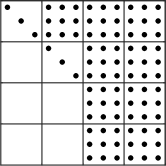
Figure 3 shows this process for a matrix with block size 3. In this figure, the continuous lines show the blocks involved in the current task, ‘’ represents a non-modified element by the current task, ‘’ represents a modified element by the current task, and ‘’ represents a nullified element by the current task. The nullified elements are shown because, as usual, they store information about the Householder transformations that will be later used to apply these transformations. The first task, called Compute_QR, computes the QR factorization of the leading dense block . The second task, called Apply_left_Qt_of_dense_QR, applies the Householder transformations obtained in the previous task (and stored in ) to block . The third task performs the same operation onto . The fourth task is the annhiliation of block , which is called Compute_td_QR (where ‘td‘ means triangular-dense). The fifth task, called Apply_left_Qt_of_td_QR, apply the transformations of the previous task to blocks and . The sixth task performs the same operation onto and . Analogously, the seventh, eighth, and ninth tasks perform the same as tasks fourth, fifth, and sixth to the first and third row of blocks. By taking advantage of the zeros present in the factorizations for each iteration, a well-implemented QR_AB cost essentially no more flops than the traditional blocked unpivoted QR. The algorithm is described in greater detail in [28, 27, 6].
4.2 Algorithms-by-blocks for randUTV
An algorithm-by-blocks for randUTV, which we will call randUTV_AB, performs mostly the same operations as the original. The key difference is that the operations’ new representations allow greater flexibility in the order of completion. We will discuss in some detail how this plays out in the first step of the algorithm. First, choose a block size (in practice, or works well). For simplicity, assume divides both and evenly. Recall that at the beginning of randUTV, is initialized with . Consider a partitioning of the matrix
where each submatrix or block is , , and . Note that the rest of matrices (, , , and ) must also be accordingly partitioned. The submatrices (and those of the rest of matrices) are treated as the fundamental unit of data in the algorithm, so that each operation is expressed only in these terms. For the first step of the algorithm, for instance:
-
1.
Constructing : The first step, is broken into several tasks that each calculate the product of two blocks. In the simplified case where , we have products of two blocks. The second step, the QR factorization of , uses an algorithm based on the idea of updating a QR factorization when more rows are added to the input matrix. Thus, the decomposition of each is computed separately, and the resulting upper triangular factor is updated after each step. See, e.g. [17, 27, 28] for details on this approach to QR factorization.
-
2.
Constructing : This step requires an unpivoted QR factorization of the same size as , so same update-based algorithm used for is used again here.
-
3.
Computing SVD of : This step is the same in randUTV and randUTV_AB. In both cases, is interacted with as a single unit.
-
4.
Updating : The rest of randUTV_AB involves the updating of , i.e. the computations and . The computations are broken down into separate stages such that the updating of each is a different task.
4.3 The FLAME abstraction for implementing algorithm-by-blocks.
A nontrivial obstacle to implementing an algorithm-by-blocks is the issue of programmability. Using the traditional approach of calls to a LAPACK implementation for the computational steps, keeping track of indexing quickly becomes complicated and error-prone.
The FLAME (Formal Linear Algebra Methods Environment) project [16, 19] is one solution to this issue. FLAME is a framework for designing linear algebraic algorithms that departs from the traditional index-based-loop methodology. Instead, the input matrix is interacted with as a collection of submatrices, basing its loops on re-partitionings of the input.
The FLAME API [4] for the C language codifies these ideas, enabling a user of the API to code high performance implementations of linear algebra algorithms at a high level of abstraction. Furthermore, the methodology of the FLAME framework, and its implementation in terms of the libflame library[35] makes it a natural fit for use with an algorithm-by-blocks. Thus, the actual code for the implementation of randUTV_AB looks very similar to the written version of the algorithm given in Figure 4.
| Algorithm: |
|---|
| Partition , , where is , has columns, has columns |
| while do |
| Determine block size Repartition , , where is , has rows, has rows |
| Continue with , , |
| endwhile |
4.4 Scheduling the operations for an algorithm-by-blocks.
The runtime system called SuperMatrix [6] is an integral part of the libflame distribution, and has been leveraged to expose and exploit task-level parallelism in in randUTV_AB. To understand how SuperMatrix schedules and executes suboperations, consider the problem of factorizing a matrix of blocks
where each block is of size . We will consider the case where the power iteration parameter for simplicity.
Execution of the program proceeds in two phases: the analysis stage and the execution stage. In the first stage, instead of executing the code sequentially, the runtime builds a list of tasks recording the dependency information associated with each operation and placing it in a queue. An example of the queue built up by the runtime for randUTV_AB for the case that and the block size is is given in Figure 5.
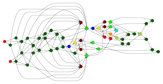
In the second stage, the scheduling/dispatching stage, the tasks in the queue are dynamically scheduled and executed. Each task is executed as soon as its input data becomes available and a core is free to complete the work. Figure 6 illustrates the execution of the first half of randUTV_AB for a matrix with block size . Figure 7 shows an actual DAG that illustrate the data dependences between tasks for the complete execution. From the code perspective, the main FLAME formulation (see Figure 4) remains unchanged, replacing the actual calls to BLAS/LAPACK codes by task definition –including input/output per-task data– and addition to the DAG. From that point on, the scheduling/dispatching stage is transparent for the developer.
| Operation | Operands | |||
| In | In/Out | |||
| Generate_normal_random | ||||
| Generate_normal_random | ||||
| Gemm_tn_oz: | ||||
| Gemm_tn_oz: | ||||
| Gemm_tn_oo: | ||||
| Gemm_tn_oo: | ||||
| Comp_dense_QR | , | |||
| Copy | ||||
| Comp_td_QR | , , | |||
| Apply_right_Q_of_dense_QR | ||||
| Apply_right_Q_of_dense_QR | ||||
| Apply_right_Q_td_QR | ||||
| Apply_right_Q_td_QR | ||||
| Comp_dense_QR | ||||
| Copy | ||||
| Comp_td_QR | ||||
| Apply_left_Qt_of_dense_QR | ||||
| Apply_left_Qt_of_td_QR | ||||
| Keep_upper_triang | ||||
| Set_to_zero | ||||
| Svd_of_block | ||||
| Gemm_abta: | ||||
| Svd_of_block | ||||
| Gemm_aabt: | ||||
| Operation | Operands | ||
|---|---|---|---|
| In | In/Out | ||
| Generate_normal_random | ✓ | ||
| Generate_normal_random | ✓ | ||
| Gemm_tn_oz: | ✓ | ✓ | |
| Gemm_tn_oz: | ✓ | ✓ | |
| Gemm_tn_oo: | ✓ | ||
| Gemm_tn_oo: | ✓ | ||
| Comp_dense_QR | , ✓ | ||
| Copy | ✓ | ||
| Comp_td_QR | , , ✓ | ||
| Apply_right_Q_of_dense_QR | ✓ | ||
| Apply_right_Q_of_dense_QR | ✓ | ||
| Apply_right_Q_td_QR | ✓ | ||
| Apply_right_Q_td_QR | ✓ | ||
| Operands | ||
|---|---|---|
| In | In/Out | |
| ✓ | ✓ | ✓ |
| ✓ | ✓ | ✓ |
| ✓ | ✓ | |
| ✓ | ✓ | |
| , ✓ | ||
| ✓ | ||
| , , ✓ | ||
| ✓ | ||
| ✓ | ||
| ✓ | ||
| ✓ | ||
| Operands | ||
|---|---|---|
| In | In/Out | |
| ✓ | ✓ | ✓ |
| ✓ | ✓ | ✓ |
| , ✓ | ||
| ✓ | ||
| , , ✓ | ||
| ✓ | ||
| ✓ | ||
| ✓ | ||
| ✓ | ||
| Operands | ||
|---|---|---|
| In | In/Out | |
| ✓, ✓ | ||
| ✓ | ||
| , ✓, ✓ | ||
| ✓ | ||
| ✓ | ||
| ✓ | ||
| ✓ | ||
| Operands | ||
|---|---|---|
| In | In/Out | |
| ✓ | ✓ | |
| , ✓, ✓ | ||
| ✓ | ✓ | |
| ✓ | ✓ | |
| ✓ | ||
| ✓ | ||
| Operands | ||
|---|---|---|
| In | In/Out | |
| ✓, ✓, ✓ | ||
| ✓ | ✓ | ✓ |
| ✓ | ✓ | ✓ |
| ✓ | ||
| ✓ | ||
| Operands | ||
|---|---|---|
| In | In/Out | |
| ✓ | ✓ | ✓ |
| ✓ | ✓ | ✓ |
5 Efficient distributed memory randUTV implementation.
Distributed memory computing architectures are commonly used for solving large problems as they extend both memory and processing power over single systems. In this section, we discuss an efficient implementation of randUTV for distributed memory. In Section 5.1, we discuss the algorithmic overview and present the software used in the implementation. Section 5.2 familiarizes the reader with ScaLAPACK’s structure and software dependencies. In Section 5.3 we review ScaLAPACK’s data distribution scheme, and in Section 5.4 we describe how the building blocks of randUTV operate in the distributed memory environment.
5.1 Implementation overview.
The distributed memory implementation of randUTV uses the standard blocked algorithm of [21] rather than the algorithm-by-blocks (as discussed in Section 4.2) since this methodology usually does not render high performances on distributed memory machines. Like in some other factorizations (QR, SVD, etc.), when applying randUTV to a matrix with , it is best to perform an unpivoted QR factorization first and then perform the randUTV factorization on the resulting square triangular factor. This method is usually applied in other architectures such as shared memory.
The ScaLAPACK software library [5, 8, 10] was used in the presented implementation. This library provides much of the functionality of LAPACK for distributed memory environments. It hides most of the communication details from the developer with an object-based API, where each matrix’s object information is passed to library routines. This design choice enhances the programmability of the library, enabling codes to be written similarly to a standard LAPACK implementation. However, as it is implemented in Fortran-77, its object orientation is not perfect and the programming effort is larger.
5.2 Software dependencies.
ScaLAPACK (scalable LAPACK) was designed to be portable to a variety of computing distributed memory architectures and relies on only two external libraries (since PBLAS is considered an internal module). The first one is the sequential BLAS (Basic Linear Algebra Subroutines) [20, 12, 11], providing specifications for the most common operations involving vectors and matrices. The second one is the BLACS (Basic Linear Algebra Communication Subroutines), which, as the name suggests, is a specification for common matrix and vector communication tasks [1].
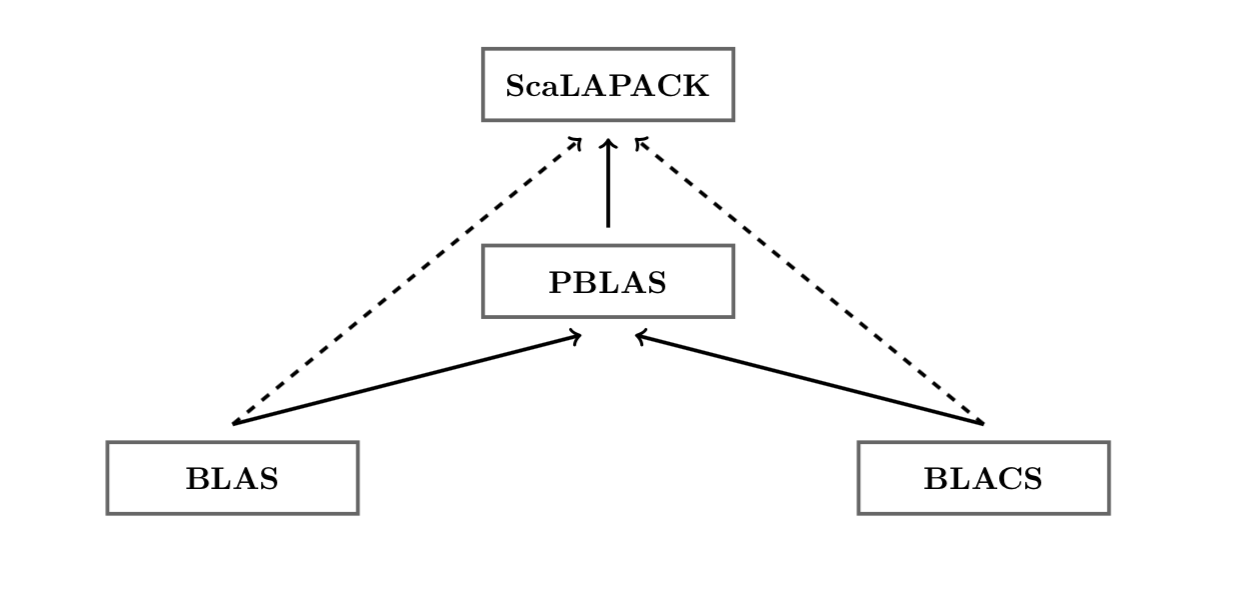
The PBLAS library is a key module inside ScaLAPACK. It comprises most of BLAS routines re-written for use in distributed memory environments. This library is written using a combination of the sequential BLAS library and the BLACS library. Just as the BLAS library contains the primary building blocks for LAPACK routines, the PBLAS library contains the foundation for the routines in ScaLAPACK. The diagram in Figure 8 illustrates the dependencies of the ScaLAPACK modules. The PBLAS library serves a dual purpose in the library. First, because the PBLAS library mirrors the sequential BLAS in function, the top level of code in main ScaLAPACK routines look largely the same as the corresponding LAPACK routines. Second, the PBLAS library adds a layer of flexibility to the code regarding the mapping of operations. Traditionally, one process is assigned to each core during execution, but with a parallel BLAS implementation, a combination of processes and threads may be used. This adjustability gives more options when mapping processes onto cores just before the program execution starts.
5.3 ScaLAPACK data distribution scheme.
The strategy for storing data in a distributed memory computation has a significant impact on the communication cost and load balance during computation. All ScaLAPACK routines assume the so-called “block-cyclic distribution” scheme [9]. Since it involves several user-defined parameters, understanding this method is vital to building an efficient implementation.
The block-cyclic distribution scheme involves four parameters. The first two, and define the block size, i.e. the dimensions of the submatrices used as the fundamental unit for communication among processes. Despite this flexibility, nearly all the main routines usually employ for the purpose of simplicity. The last two parameters, typically called and , determine the shape of the logical process grid.
To understand which elements of the input matrix are stored in which process, we may visualize the matrix as being partitioned into “tiles.” In the simple case where and divide and , respectively, every tile is of uniform size. Each tile is composed of blocks, each of size . Finally, every process is assigned a position on the tile grid. The block in that position on every tile is stored in the corresponding process. For example, the block in the spot in each tile belongs with the first process , the block in the spot in each tile belongs to the second process , and so on. An example is given in Figure 9 to demonstrate this.

5.4 Building blocks of randUTV
In this section we examine further the randUTV algorithm in order to understand which portions of the computation are most expensive (when no orthonormal matrices are built) and how these portions perform in the distributed memory environment. Judging by numbers of flops required, the three portions of the computation that take the most time are the following:
-
1.
applying stage to ,
-
2.
applying stage to ,
-
3.
building .
To determine the fundamental operations involved in items 1 and 2, first recall that and are both formed from a Householder reduction on matrices with columns to upper trapezoidal form. As such, we may express them in the so-called compact form (see Section 2.3) as
where are upper triangular, and and are lower trapezoidal. Thus the computations and each require three matrix-matrix multiplications where one dimension of the multiplication is small (recall ). Note that the first computation () is more expensive than the second one () because the first one processes all the rows of (the right part of ), whereas the second one only processes some rows of (the bottom right part of ).
It is now evident that items 1 and 2 use primarily xgemm and xtrmm from the BLAS. Furthermore, item 3 is strictly a series of xgemm operations, so we see that matrix-matrix multiplications form the dominant cost within randUTV.
xgemm for distributed memory, which in the PBLAS library is titled pxgemm, is well-suited for efficiency in this environment. In the reference implementation of PBLAS, pxgemm may execute one of three different algorithms for matrix multiplication:
-
1.
pxgemmAB: The outer-product algorithm is used; matrix remains in place.
-
2.
pxgemmBC: The inner-product algorithm is used; matrix remains in place.
-
3.
pxgemmAC: The inner-product algorithm is used; matrix remains in place.
xgemm chooses among the algorithms by estimating the communication cost for each, depending on matrix dimensions and parameters of the storage scheme. The inherent flexibility of the matrix-matrix multiply enables good pxgemm implementations to overlap the communication with the processing of flops. Thus, randUTV for distributed memory obtains better speedups when more cores are added than competing implementations of SVD and CPQR algorithms for distributed memory.
6 Performance analysis
In this section, we investigate the speed of our new implementations of the algorithm for computing the randUTV factorization, and compare it to the speeds of highly optimized methods for computing the SVD and the column pivoted QR (CPQR) factorization. In all the experiments double-precision real matrices were processed.
To fairly compare the different implementations being assessed, the flop count or the usual flop rate could not be employed since the computation of the SVD, the CPQR, and the randUTV factorizations require a very different number of flops (the dominant -term in the asymptotic flop count is very different). Absolute computational times are not shown either since they vary greatly because of the large range of matrix dimensions employed in the experiments. Therefore, scaled computational times (absolute computational times divided by ) are employed. Hence, the lower the scaled computational times, the better the performances are. Since all the implementations being assessed have asymptotic complexity when applied to an matrix, these graphs better reveal the computational efficiency. Those scaled times are multiplied by a constant (usually ) to make the figures in the vertical axis more readable.
Although most of the plots show scaled computational times, a few plots show speedups. The speedup is usually computed as the quotient of the time obtained by the serial implementation (on one core) and the time obtained by the parallel implementation (on many cores). Thus, this concept communicates how many times faster the parallel implementation is compared to the serial one. Hence, the higher the speedups, the better the performances of the parallel implementation are. This measure is usually very useful in checking the scalability of an implementation. Note that in this type of plots every implementation compares against itself on one core.
6.1 Computational speed on shared-memory architectures
We employed the following two computers in the experiments with shared-memory architectures:
-
•
marbore: It featured two Intel Xeon® CPUs E5-2695 v3 (2.30 GHz), with 28 cores and 128 GiB of RAM in total. In this computer the so-called Turbo Boost mode of the two CPUs was turned off in our experiments.
Its OS was GNU/Linux (Kernel Version 2.6.32-504.el6.x86_64). GCC compiler (version 6.3.0 20170516) was used. Intel(R) Math Kernel Library (MKL) Version 2018.0.1 Product Build 20171007 for Intel(R) 64 architecture was employed since LAPACK routines from this library usually deliver much higher performances than LAPACK routines from the Netlib repository.
Unless explicitly stated otherwise, experiments have been run in this machine since it was not so busy.
-
•
mimir: It featured two Intel Xeon® CPUs Gold 6254 (3.10 GHz), with 36 cores and 791 GB of RAM in total. The Max Turbo Frequency of the CPUs was 4.00 GHz.
Its OS was GNU/Linux (Kernel Version 5.0.0-32-generic). Intel C compiler (version 19.0.5.281 20190815) was used. Intel(R) Math Kernel Library (MKL) Version 2019.0.5 Product Build 20190808 for Intel(R) 64 architecture was employed because of the same reason as above.
When using routines of MKL’s LAPACK, optimal block sizes determined by that software were employed. In a few experiments, in addition to MKL’s LAPACK routines, we also assessed Netlib’s LAPACK 3.4.0 routines. In this case, the Netlib term is used. When using routines of Netlib’s LAPACK, several block sizes were employed and best results were reported. For the purpose of a fair comparison, these routines from Netlib were linked to the BLAS library from MKL.
All the matrices used in the experiments were randomly generated. Similar results for randUTV were obtained on other types of matrices, since one of the main advantages of the randTUV algorithm is that its performances do not depend on the matrix being factorized.
Unless explicitely stated otherwise, all the experiments employed the 28 cores in the computer.
The following implementations were assessed in the experiments of this subsection:
-
•
MKL SVD: The routine called dgesvd from MKL’s LAPACK was used to compute the Singular Value Decomposition.
-
•
Netlib SVD: Same as the previous one, but the code for computing the SVD from Netlib’s LAPACK was employed, instead of MKL’s.
-
•
MKL SDD: The routine called dgesdd from MKL’s LAPACK was used to compute the Singular Value Decomposition. Unlike the previous SVD, this one uses the divide-and-conquer approach. This code is usually faster, but it requires a much larger auxiliary workspace when the orthonormal matrices are built (about four additional matrices of the same dimension as the matrix being factorized).
-
•
Netlib SDD: Same as the previous one, but the code for computing the SVD with the divide-and-conquer approach from Netlib’s LAPACK was employed, instead of MKL’s.
-
•
MKL CPQR: The routine called dgeqp3 from MKL’s LAPACK was used to compute the column-pivoting QR factorization.
-
•
randUTV PBLAS (randUTV with parallel BLAS): This is the traditional implementation for computing the randUTV factorization that relies on the parallel BLAS to take advantage of all the cores in the system. The parallel BLAS library from MKL was employed with these codes for the purpose of a fair comparison. Our implementations were coded with libflame [36, 35] (Release 11104).
-
•
randUTV AB (randUTV with Algorithm-by-Blocks): This is the new implementation for computing the randUTV factorization by scheduling all the tasks to be computed in parallel, and then executing them with serial BLAS. The serial BLAS library from MKL was employed with these new codes for the purpose of a fair comparison. Our implementations were coded with libflame [36, 35] (Release 11104).
-
•
MKL QR: The routine called dgeqrf from MKL’s LAPACK was used to compute the QR factorization. Although this routine does not reveal the rank, it was included in some experiments as a performance reference for the others.
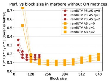
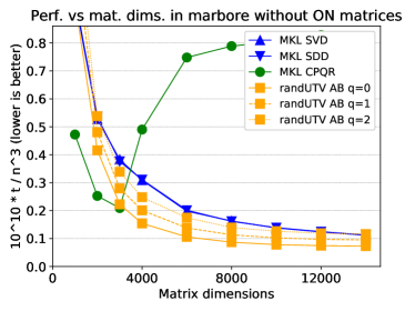
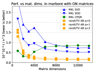
For every experiment, two plots are shown. The left plot shows the performances when no orthonormal matrices are computed. In this case, just the singular values are computed for the SVD, just the upper triangular factor is computed for the CPQR and the QR, and just the upper triangular factor is computed for the randUTV. In contrast, the right plot shows the performances when all orthonormal matrices are explicitly formed in addition to the singular values (SVD), the upper triangular matrix (CPQR), or the upper triangular matrix (randUTV). In this case, matrices and are computed for the SVD and the randUTV, and matrix is computed for the CPQR and the QR. The right plot slightly favors CPQR and QR since only one orthonormal matrix is formed.
 |
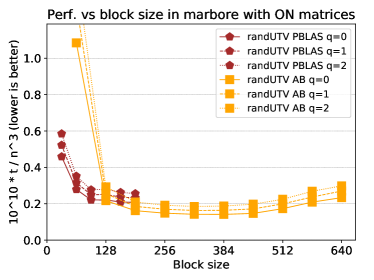 |
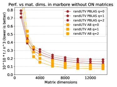
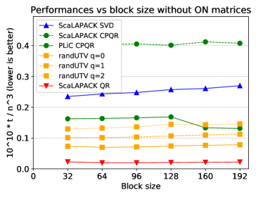
Figure 10 shows the scaled computational times obtained by both implementations for computing the randUTV factorization (randUTV PBLAS and randUTV AB) on several block sizes when processing matrices of dimension . The aim of these two plots is to determine the optimal block sizes. The other factorizations (SVD and CPQR) are not shown since in those cases we used the optimal block sizes determined by Intel’s software. Optimal block sizes were around 128 for randUTV PBLAS; on the other hand, optimal block sizes were around 384 for randUTV AB.
 |
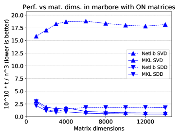 |
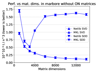
Figure 11 compares the performances of four implementations for computing the SVD factorization: MKL SVD (usual SVD from the MKL library), MKL SDD (divide-and-conquer SVD from the MKL library), Netlib SVD (usual SVD from the Netlib library), and Netlib SDD (divide-and-conquer SVD from the Netlib library). Performances are shown with respect to matrix dimensions. Block sizes similar to those in the previous figure were used for Netlib’s routines and the best results were reported. When no orthonormal matrices are computed, both the traditional SVD and the divide-and-conquer SVD render similar performances for this matrix type. In this case, MKL routines are up to 14.1 times as fast as Netlib’s routines. When orthonormal matrices are computed, the traditional SVD is much slower than the divide-and-conquer SVD. In this case, the MKL SVD routine is up to 24.4 times as fast as the Netlib SVD, and the MKL SDD routine is up to 3.4 times as fast as the Netlib SDD. As can be seen, MKL’s codes for computing the SVD are up to more than one order of magnitude faster than Netlib’s codes, thus showing the great performances achieved by Intel. This is a remarkable achievement for so complex codes. Outperforming these highly optimized codes can be really a difficult task.
 |
 |
Figure 12 compares the performances of both implementations of randUTV (randUTV PBLAS and randUTV AB) as a function of matrix dimensions. In both implementations, several block sizes were tested (see above), and best results were reported. When no orthonormal matrices are built, randUTV AB is between 1.80 () and 2.54 () times as fast as randUTV PBLAS for the largest matrix size. When orthonormal matrices are built, randUTV AB is between 1.73 () and 1.80 () times as fast as randUTV PBLAS for the largest matrix size.
 |
 |
 |
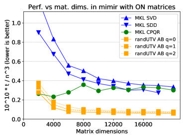 |
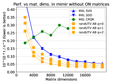
Figure 13 shows the performances of the best implementations as a function of the matrix dimensions. The top row shows results for marbore with 28 cores, whereas the bottom row shows results for mimir with 36 cores. When no orthonormal matrices are built on marbore, randUTV AB is between 1.54 () and 0.97 () times as fast as MKL SVD for the largest matrix size. When no orthonormal matrices are built on mimir, randUTV AB is between 1.77 () and 1.15 () times as fast as MKL SVD for the largest matrix size. When orthonormal matrices are built on marbore, randUTV AB is between 3.65 () and 2.79 () times as fast as MKL SVD for the largest matrix size. When orthonormal matrices are built on mimir, randUTV AB is between 5.65 () and 4.39 () times as fast as MKL SVD for the largest matrix size. The previous comparisons have been done against MKL SVD since MKL SDD could not be executed on because of its larger memory requirements for workspace. Recall that this driver requires a much larger auxiliary workspace than randUTV AB (about four times as large as the original matrix). The speeds of randUTV AB, MKL SVD and MKL SDD are so remarkable that they are similar or even much faster than MKL CPQR, a factorization that requires much fewer flops.
 |
 |
 |
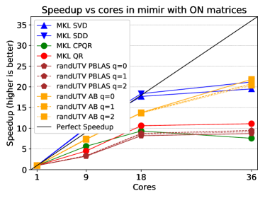 |
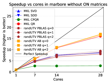
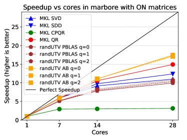
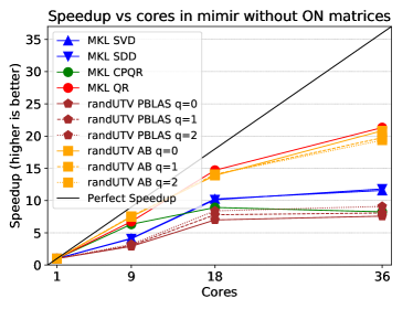
Figure 14 shows the speedups obtained by the best implementations on both machines. The top row shows results of marbore on matrices of dimension , whereas the bottom row shows results of mimir on matrices of dimension (the largest dimension in which all the best implementations could be run). Recall that in this plot every implementation compares against itself on one core.
We see that the scalability of randUTV AB is always similar or even better than the scalability of the highly efficient unpivoted QR factorization, and it does not depend on whether the orthonormal matrices are built. Note that it always grows whenever more cores are employed. In contrast, the SVD factorizations perform very well in one case (even with a slight superspeedup): when orthonormal matrices are built using 18 cores or fewer in mimir. In all the other cases, the speedups are not so good, and the scalability even drops (the speedups do not grow much) when going from half the number of cores to the full number of cores.
As can be seen, randUTV AB is the only factorization that achieves an efficiency similar or higher than 50 % (the speedups are higher than half the number of cores) when employing the maximum number of cores in both architectures, whereas the efficiency of all the other factorizations are usually always lower. To conclude this analysis, the scalability of randUTV AB is similar (or even better) to that of the QR factorization, and much higher than the rest of the implementations.
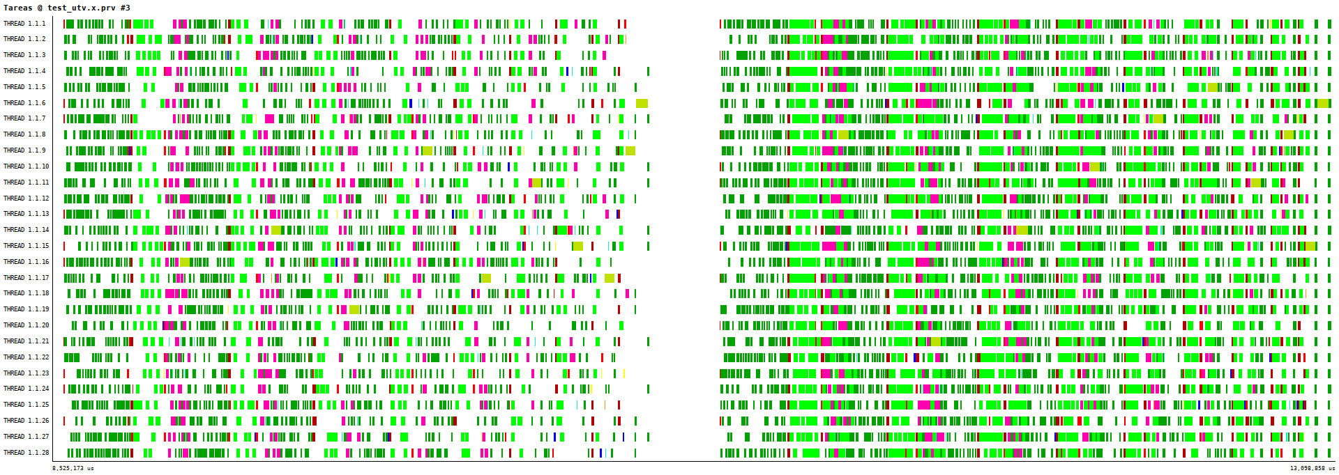
Figure 15 reports an actual execution trace for an experiment on marbore for and running on 28 cores, for a factorization that does not compute orthonormal matrices (left part of the trace) and computing orthonormal matrices (right part of the trace). Each row in the trace correspond to a worker thread; colors match those depicted in Table 5.
In conclusion, randUTV AB is the clear winner over competing factorization methods in terms of raw speed when orthonormal matrices are required and the matrix is not too small (). In terms of scalability, randUTV AB outperforms the competition as well. Also, the algorithm-by-blocks implementation gives noticeable speedup over the blocked PBLAS version. That randUTV AB can compete with MKL SVD at all in terms of speed is remarkable, given the large effort usually invested by Intel on its sofware. This is evidenced by the fact that the MKL CPQR is left in the dust by both MKL SVD and randUTV AB, each of which costs far more flops than MKL CPQR. The scalability results of randUTV AB and its excellent timings evince its potential as a high performance tool in shared memory computing.
6.2 Computational speed on distributed-memory architectures
The experiments on distributed-memory architectures reported in this subsection were performed on a cluster of HP computers. Each node of the cluster contained two Intel Xeon® CPU X5560 processors at 2.8 GHz, with 12 cores and 48 GiB of RAM in total. The nodes were connected with an Infiniband 4X QDR network. This network is capable of supporting 40 Gb/s signaling rate, with a peak data rate of 32 Gb/s in each direction.
Its OS was GNU/Linux (Version 3.10.0-514.21.1.el7.x86_64). Intel’s ifort compiler (Version 12.0.0 20101006) was employed. LAPACK and ScaLAPACK routines were taken from the Intel(R) Math Kernel Library (MKL) Version 10.3.0 Product Build 20100927 for Intel(R) 64 architecture, since this library usually delivers much higher performances than LAPACK and ScaLAPACK codes from the Netlib repository.
All the matrices used in these experiments were randomly generated since they are much faster to be generated, and the cluster was being heavily loaded by other users.
The following implementations were assessed in the experiments of this subsection:
-
•
ScaLAPACK SVD: The routine called pdgesvd from MKL’s ScaLAPACK is used to compute the Singular Value Decomposition (SVD).
-
•
ScaLAPACK CPQR: The routine called pdgeqpf from MKL’s ScaLAPACK is used to compute the column-pivoted QR factorization.
-
•
PLiC CPQR: The routine called pdgeqp3 from the PLiC library (Parallel Library for Control) [3] is used to compute the column-pivoted QR factorization by using BLAS-3. This source code was linked to the ScaLAPACK library from MKL for the purpose of a fair comparison.
-
•
randUTV: A new implementation for computing the randUTV factorization based on the ScaLAPACK infrastructure and library. This source code was linked to the ScaLAPACK library from MKL for the purpose of a fair comparison.
-
•
ScaLAPACK QR: The routine called dgeqrf from MKL’s ScaLAPACK is used to compute the QR factorization. Although this routine does not reveal the rank, it was included in some experiments as a reference for the others.
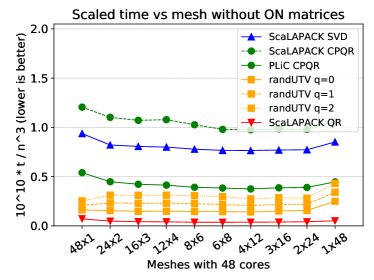
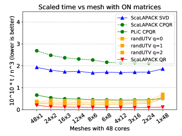
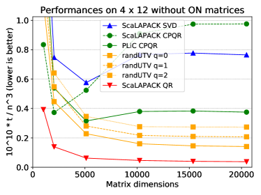
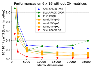
Like in the previous subsection on shared-memory architectures, for every experiment two plots are shown. The left plot shows the performances when no orthonormal matrices are computed (the codes compute just the singular values for the SVD, the upper triangular matrix for the CPQR and the QR factorizations, and the upper triangular matrix for the randUTV factorization). The right plot shows the performances when, in addition to those, all orthonormal matrices are explicitly formed (matrices and for SVD and randUTV, and matrix for QR and CPQR). Recall that the right plot slightly favors CPQR and QR since only one orthonormal matrix is built.
 |
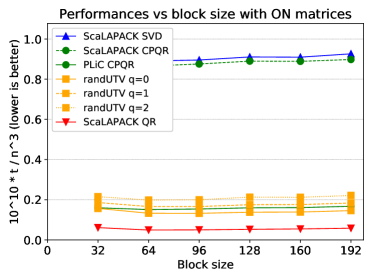 |
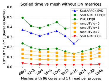
Figure 16 shows the performances of all the implementations described above on several block sizes when using 96 cores arranged as a mesh on matrices of dimension . As can be seen, most implementations perform slightly better on small block sizes, such as 32 and 64, the only exception being PLiC CPQR, which performs a bit better on large block sizes when no orthonormal matrices are built.
 |
 |
 |
 |
 |
 |
 |
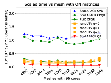 |
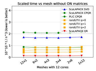
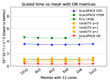
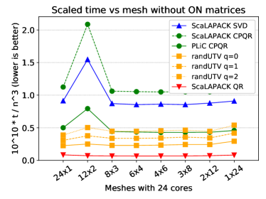
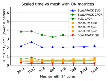
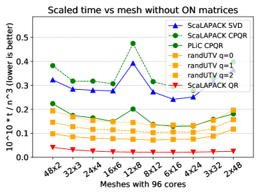
Figure 17 shows the performances of all the implementations for many topologies on matrices of dimension . The top row shows the results on one node (12 cores), the second row shows the results on two nodes (24 cores), the third row shows the results on four nodes (48 cores), and the fourth row shows the results on eight nodes (96 cores). As can be seen, best topologies are usually with slightly smaller than .
 |
 |
 |
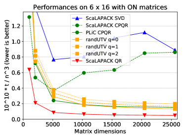 |
Figure 18 shows the performances versus matrix dimensions on two different number of cores: 48 cores arranged as (top row) and 96 cores arranged as (bottom row). On the largest matrix dimension on 48 cores, when no orthonormal matrices are built, randUTV is between 5.4 () and 2.8 () times as fast as the SVD, whereas when orthonormal matrices are built, randUTV is between 6.6 () and 4.3 () times as fast as the SVD. On the largest matrix dimension on 96 cores, when no orthonormal matrices are built, randUTV is between 3.4 () and 1.8 () times as fast as the SVD, whereas when orthonormal matrices are built, randUTV is between 6.7 () and 4.5 () times as fast as the SVD. On medium and large matrices, performances of ScaLAPACK CPQR are much lower than those of randUTV, whereas performances of PLiC CPQR are more similar to those of randUTV. Nevertheless, recall that the precision of CPQR is usually much smaller than that of randUTV.
In distributed-memory applications the traditional approach creates one process per core. However, creating fewer processes and then a corresponding number of threads per process can improve performances in some cases. Obviously, the product of the number of processes and the number of threads per process must be equal to the total number of cores. The advantage of this approach is that the creation of fewer processes reduces the communication cost, which is usually the main bottleneck in distributed-memory applications. In the case of linear algebra applications, creating and using several threads per process can be easily achieved by employing shared-memory parallel LAPACK and BLAS libraries. Nevertheless, great care must be taken to ensure a proper pinning of processes to cores, since otherwise performances drop markedly. This was achieved by using the -genv I_MPI_PIN_DOMAIN socket flag when executing the mpirun/mpiexec command in the machine used in the experiments.
 |
 |
 |
 |
 |
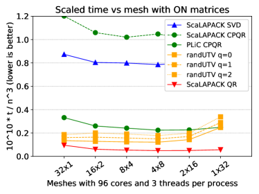 |
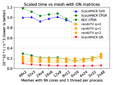
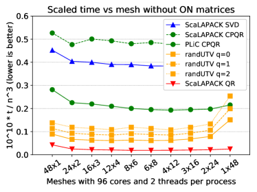
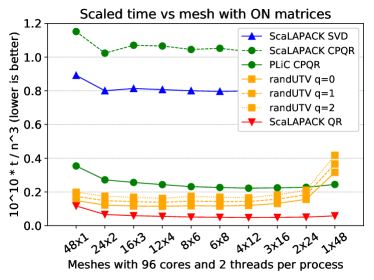
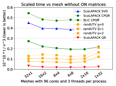
Figure 19 shows the scaled timings of the factorizations of matrices of dimension on 96 cores when using several configurations with different numbers of threads per process. These plots include the results on a complete set of topologies to isolate the effect of the increased number of threads. As usual, the left three plots show performances when no orthonormal matrices are built, whereas the right three plots show performances when orthonormal matrices are built. The top row shows performances when one process per core (96 processes) and then one thread per process are created (). The second row shows performances when one process per two cores (48 processes) and then two threads per process are created (). The third row shows performances when one process per three cores (32 processes) and then three threads per process are created (). As can be seen, the SVD only increases performances when orthonormal matrices are created, whereas randUTV increases performances in both cases (both with and without orthonormal matrices).
| No ON matrices | ON matrices | |||||
|---|---|---|---|---|---|---|
| Threads per process | Threads per process | |||||
| Factorization | 1 | 2 | 3 | 1 | 2 | 3 |
| SVD | 393.9 | 644.0 | 645.3 | 1494.1 | 1336.4 | 1318.0 |
| randUTV | 117.0 | 102.7 | 112.2 | 214.2 | 192.3 | 203.7 |
| randUTV | 168.6 | 142.5 | 160.1 | 272.1 | 232.3 | 251.4 |
| randUTV | 216.7 | 180.4 | 207.8 | 327.5 | 271.7 | 298.7 |
Table 1 shows the best timings (in seconds) for several topologies with 96 cores so a finer detail comparison can be achieved. Matrices being factorized are . As can be seen, SVD increases performances 13 % when orthonormal matrices are built, whereas randUTV with improves performances 20 % in both cases. Performances usually increase when using two threads per process, but they remain similar or drop when using more than two threads per process.
 |
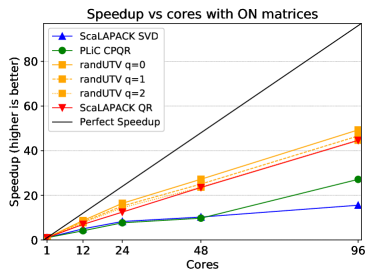 |
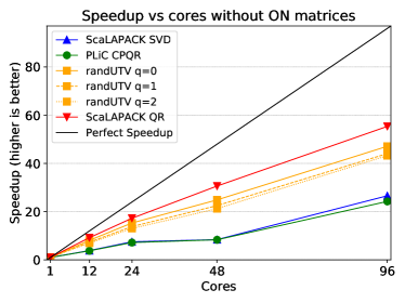
Figure 20 shows the speedups obtained by all the implementations on matrices of dimension . Recall that in this plot every implementation compares against itself on one core. The best topologies have been selected for the following number of cores: for 12 cores, for 24 cores, for 48 cores, and for 96 cores. When no orthonormal matrices are built, speedups of randUTV on the largest number of cores (96) are between 47.1 () and 43.3 (). When orthonormal matrices are built, speedups of randUTV on the largest number of cores (96) are between 49.3 () and 44.7 (). In both cases, the efficiency is close to 50 %. When no orthonormal matrices are built, speedups of randUTV are a bit lower than those of QR factorization; when orthonormal matrices are built, speedups of randUTV are a bit higher than those of QR factorization. In both cases, the speedups of randUTV are much higher than those obtained by the SVD and the CPQR factorization, thus showing the great scalability potential of this factorization.
In conclusion, randUTV is significantly faster than the available distributed memory implementations of SVD. It also matches the best CPQR implementation tested. randUTV is known to reveal rank far better than CPQR [21], and it also furnishes orthonormal bases for the row-space, and for the (numerical) null-space of the matrix. This means that just matching the speed of CPQR represents a major gain in information at no additional computational cost. Furthermore, randUTV is faster than even CPQR in the case that orthonormal matrices are required. We finally observe that the potential for scalability of randUTV is a clear step above competing implementations for rank-revealing factorizations in distributed memory.
7 Conclusions.
We have described two new implementations of the randUTV algorithm for computing the SVD of a matrix, targeting shared-memory and distributed-memory architectures, respectively.
Regarding shared memory, the new implementation proposes an algorithm-by-blocks that, built on top of a runtime task scheduler (libflame’s SuperMatrix) implements a dataflow execution model. Based on a DAG, this model reduces the amount of synchronization points and hence increases performance on massively parallel architectures. Actually, performance results on a up to 36 cores reveal excellent performance and scalability results compared with state-of-the-art proprietary libraries.
We have also proposed a distributed-memory algorithm for randUTV. This proposal leverages the classic blocked algorithm rather than the algorihm-by-blocks, and makes heavy use of ScaLAPACK. Performance results show competitive performance and excellent scalability compared with alternative state-of-the-art implementations.
In this article, we focused exclusively on the case of multicore CPUs with shared memory and homogeneous distributed-memory architectures. We expect that the relative advantages of randUTV will be even more pronounced in more severely communication- constrained environments, such as GPU-based architectures (composed by one or many nodes). Work on variations of the method modied for such environments is proposed as future work.
Acknowledgements
F. D. Igual was supported by the EU (FEDER) and Spanish MINECO (GA No. RTI2018-093684-B-I00), and by Spanish CM (GA No. S2018/TCS-4423).
G. Quintana-Ortí was supported by the Spanish Ministry of Science, Innovation and Universities under Grant RTI2018-098156-B-C54 co-financed with FEDER funds.
P. G. Martinsson was supported by the Office of Naval Research (grant N00014-18-1-2354) and by the National Science Foundation (grant DMS-1620472).
The authors would also like to thank Javier Navarrete (Universitat d’Alacant) for granting access to the distributed-memory server.
References
- [1] Ed Anderson, A Benzoni, J Dongarra, S Moulton, S Ostrouchov, Bernard Tourancheau, and Robert van de Geijn, Basic linear algebra comrnunication subprograms, The Sixth Distributed Memory Computing Conference, 1991. Proceedings, IEEE, 1991, pp. 287–290.
- [2] Jesse L Barlow, Modification and maintenance of ulv decompositions, Applied Mathematics and Scientific Computing, Springer, 2002, pp. 31–62.
- [3] Peter Benner, Enrique S. Quintana-Ortí, and Gregorio Quintana-Ortí, Solving linear-quadratic optimal control problems on parallel computers, Optimization Methods and Software 23 (2008), no. 6, 879–909.
- [4] Paolo Bientinesi, Enrique S Quintana-Ortí, and Robert A Geijn, Representing linear algebra algorithms in code: the flame application program interfaces, ACM Transactions on Mathematical Software (TOMS) 31 (2005), no. 1, 27–59.
- [5] L Susan Blackford, Jaeyoung Choi, Andy Cleary, Eduardo D’Azevedo, James Demmel, Inderjit Dhillon, Jack Dongarra, Sven Hammarling, Greg Henry, Antoine Petitet, et al., Scalapack users’ guide, SIAM, 1997.
- [6] Ernie Chan, Enrique S Quintana-Orti, Gregorio Quintana-Orti, and Robert Van De Geijn, Supermatrix out-of-order scheduling of matrix operations for smp and multi-core architectures, Proceedings of the nineteenth annual ACM symposium on Parallel algorithms and architectures, ACM, 2007, pp. 116–125.
- [7] Ernie Chan, Field G. Van Zee, Paolo Bientinesi, Enrique S. Quintana-Orti, Gregorio Quintana-Orti, and Robert van de Geijn, Supermatrix: a multithreaded runtime scheduling system for algorithms-by-blocks, Proceedings of the 13th ACM SIGPLAN Symposium on Principles and practice of parallel programming (New York, NY, USA), PPoPP ’08, ACM, 2008, pp. 123–132.
- [8] Jaeyoung Choi, James Demmel, Inderjiit Dhillon, Jack Dongarra, Susan Ostrouchov, Antoine Petitet, Ken Stanley, David Walker, and R Clinton Whaley, Scalapack: A portable linear algebra library for distributed memory computers?design issues and performance, Computer Physics Communications 97 (1996), no. 1-2, 1–15.
- [9] Jaeyoung Choi, Jack J Dongarra, L Susan Ostrouchov, Antoine P Petitet, David W Walker, and R Clint Whaley, Design and implementation of the scalapack lu, qr, and cholesky factorization routines, Scientific Programming 5 (1996), no. 3, 173–184.
- [10] Jaeyoung Choi, Jack J Dongarra, Roldan Pozo, and David W Walker, Scalapack: A scalable linear algebra library for distributed memory concurrent computers, Frontiers of Massively Parallel Computation, 1992., Fourth Symposium on the, IEEE, 1992, pp. 120–127.
- [11] Jack J Dongarra, Jermey Du Cruz, Sven Hammarling, and Iain S Duff, Algorithm 679: A set of level 3 basic linear algebra subprograms: model implementation and test programs, ACM Transactions on Mathematical Software (TOMS) 16 (1990), no. 1, 18–28.
- [12] Jack J Dongarra, Jeremy Du Croz, Sven Hammarling, and Richard J Hanson, Algorithm 656: an extended set of basic linear algebra subprograms: model implementation and test programs, ACM Transactions on Mathematical Software (TOMS) 14 (1988), no. 1, 18–32.
- [13] Carl Eckart and Gale Young, The approximation of one matrix by another of lower rank, Psychometrika 1 (1936), no. 3, 211–218.
- [14] Hasan Erbay, Jesse L Barlow, and Zhenyue Zhang, A modified gram–schmidt-based downdating technique for ulv decompositions with applications to recursive tls problems, Computational statistics & data analysis 41 (2002), no. 1, 195–209.
- [15] Gene H. Golub and Charles F. Van Loan, Matrix computations, third ed., Johns Hopkins Studies in the Mathematical Sciences, Johns Hopkins University Press, Baltimore, MD, 1996.
- [16] John A Gunnels, Fred G Gustavson, Greg M Henry, and Robert A Van De Geijn, Flame: Formal linear algebra methods environment, ACM Transactions on Mathematical Software (TOMS) 27 (2001), no. 4, 422–455.
- [17] Brian C Gunter and Robert A Van De Geijn, Parallel out-of-core computation and updating of the qr factorization, ACM Transactions on Mathematical Software (TOMS) 31 (2005), no. 1, 60–78.
- [18] Nathan Halko, Per-Gunnar Martinsson, and Joel A. Tropp, Finding structure with randomness: Probabilistic algorithms for constructing approximate matrix decompositions, SIAM Review 53 (2011), no. 2, 217–288.
- [19] Francisco D Igual, Ernie Chan, Enrique S Quintana-Ortí, Gregorio Quintana-Ortí, Robert A Van De Geijn, and Field G Van Zee, The flame approach: From dense linear algebra algorithms to high-performance multi-accelerator implementations, Journal of Parallel and Distributed Computing 72 (2012), no. 9, 1134–1143.
- [20] Chuck L Lawson, Richard J. Hanson, David R Kincaid, and Fred T. Krogh, Basic linear algebra subprograms for fortran usage, ACM Transactions on Mathematical Software (TOMS) 5 (1979), no. 3, 308–323.
- [21] P. G. Martinsson, G. Quintana-Ortí, and N. Heavner, Randutv: A blocked randomized algorithm for computing a rank-revealing utv factorization, ACM Trans. Math. Softw. 45 (2019), no. 1.
- [22] Per-Gunnar Martinsson, Vladimir Rokhlin, and Mark Tygert, A randomized algorithm for the approximation of matrices, Tech. Report Yale CS research report YALEU/DCS/RR-1361, Yale University, Computer Science Department, 2006.
- [23] , A randomized algorithm for the decomposition of matrices, Appl. Comput. Harmon. Anal. 30 (2011), no. 1, 47–68. MR 2737933 (2011i:65066)
- [24] Per-Gunnar Martinsson and Joel Tropp, Randomized numerical linear algebra: Foundations & algorithms, 2020.
- [25] Leon Mirsky, Symmetric gauge functions and unitarily invariant norms, The quarterly journal of mathematics 11 (1960), no. 1, 50–59.
- [26] Haesun Park and Lars Eldén, Downdating the rank-revealing urv decomposition, SIAM Journal on Matrix Analysis and Applications 16 (1995), no. 1, 138–155.
- [27] Gregorio Quintana-Ortí, Francisco D Igual, Mercedes Marqués, Enrique S Quintana-Ortí, and Robert A Van de Geijn, A runtime system for programming out-of-core matrix algorithms-by-tiles on multithreaded architectures, ACM Transactions on Mathematical Software (TOMS) 38 (2012), no. 4, 25.
- [28] Gregorio Quintana-Ortí, Enrique S. Quintana-Ortí, Robert A. Van De Geijn, Field G. Van Zee, and Ernie Chan, Programming matrix algorithms-by-blocks for thread-level parallelism, ACM Trans. Math. Softw. 36 (2009), no. 3, 14:1–14:26.
- [29] Vladimir Rokhlin, Arthur Szlam, and Mark Tygert, A randomized algorithm for principal component analysis, SIAM Journal on Matrix Analysis and Applications 31 (2009), no. 3, 1100–1124.
- [30] Robert Schreiber and Charles Van Loan, A storage-efficient wy representation for products of householder transformations, SIAM Journal on Scientific and Statistical Computing 10 (1989), no. 1, 53–57.
- [31] G. W. Stewart, An updating algorithm for subspace tracking, IEEE Transactions on Signal Processing 40 (1992), no. 6, 1535–1541.
- [32] Gilbert W Stewart, Updating a rank-revealing ulv decomposition, SIAM Journal on Matrix Analysis and Applications 14 (1993), no. 2, 494–499.
- [33] G.W. Stewart, Matrix algorithms volume 1: Basic decompositions, SIAM, 1998.
- [34] Lloyd N Trefethen and David Bau III, Numerical linear algebra, vol. 50, Siam, 1997.
-
[35]
Field G. Van Zee, libflame: The Complete Reference, www.lulu.com, 2012,
Download from http://www.cs.utexas.edu/users/flame/web/FLAMEPublications.html. - [36] Field G. Van Zee, Ernie Chan, Robert van de Geijn, Enrique S. Quintana-Ortí, and Gregorio Quintana-Ortí, The libflame library for dense matrix computations, IEEE Computation in Science & Engineering 11 (2009), no. 6, 56–62.