Observation of phase synchronization and alignment during free induction decay of quantum spins with Heisenberg interactions

Abstract

Equilibration of observables in closed quantum systems that are described by a unitary time evolution is a meanwhile well-established phenomenon apart from a few equally well-established exceptions. Here we report the surprising theoretical observation that integrable as well as non-integrable spin rings with nearest-neighbor or long-range isotropic Heisenberg interaction not only equilibrate but moreover also synchronize the directions of the expectation values of the individual spins. We highlight that this differs from spontaneous synchronization in quantum dissipative systems. Here, we observe mutual synchronization of local spin directions in closed systems under unitary time evolution. Contrary to dissipative systems, this synchronization is independent of whether the interaction is ferro- or antiferromagnetic. In our numerical simulations, we investigate the free induction decay (FID) of an ensemble of up to $N=25$ quantum spins with $s=1/2$ each by solving the time-dependent Schrödinger equation numerically exactly. Our findings are related to, but not fully explained by conservation laws of the system. The synchronization is very robust against for instance random fluctuations of the Heisenberg couplings and inhomogeneous magnetic fields. Synchronization is not observed with strong enough symmetry-breaking interactions such as the dipolar interaction. We also compare our results to closed-system classical spin dynamics which does not exhibit phase synchronization due to the lack of entanglement. For classical spin systems the fixed magnitude of individual spins effectively acts like additional $N$ conservation laws.

I Introduction

Decoherence, equilibration as well as thermalization in closed quantum systems under unitary time evolution are well-studied and by now well-established concepts which root in seminal papers by Deutsch, Srednicki and many others [1, 2, 3, 4, 5, 6, 7, 8, 9, 10, 11, 12]. For numerical studies, spin systems are the models of choice both since they are numerically feasible due to the finite size of their Hilbert spaces as well as they are experimentally accessible for instance in standard investigations by means of electron parametric resonance (EPR), free induction decay (FID), or in atomic traps, see e.g. [13, 14, 15, 16, 17]. In such systems, observables assume expectation values that are practically indistinguishable from the prediction of the diagonal ensemble for the vast majority of all times of their time evolution [6, 18].

In this paper we discuss an observation that rests both on decoherence and equilibration. We study the free induction decay (FID) of quantum spins that are arranged on a ring-like geometry with nearest-neighbor as well as long-range isotropic Heisenberg interactions. For the overwhelming majority of investigated cases the initial product state of single-spin states entangles, i.e. turns into a superposition of product states, and thereby equilibrates at the level of single-spin observables. Our most striking observation is that expectation values of all individual spin vectors synchronize with respect to their orientation. In a FID setting this means that their various individual rotations about the common field axis synchronize and align in the course of time. In a co-rotating frame they simply align. Experimentally, such collective effects may e.g. be imprinted in the temporal line shapes of the optical response under ultrashort pulse excitation and thus eventually be observed [19].

We would like to contrast our findings with the longer-known observation of (spontaneous) synchronization in dissipative systems [20, 21, 22, 23, 24]. It was controversially discussed whether quantum two-level systems are able to synchronize at all [25], with later conclusions that this is indeed the case [26, 22]. All these investigations have in common that they try to identify stable limit cycles of the participating oscillators. Since such a discussion is applicable only to dissipative systems, which can emit or absorb energy to return to their stable oscillation after a perturbation, it probably cannot serve as an explanation in our case.

A related and already investigated topic is transient synchronization in open quantum systems [27], in which the system finally equilibrates to a non-synchronized state, but synchronizes temporarily on the way. We show that we observe a comparable behavior in closed quantum spin systems, if we weakly reduce the symmetry of the Hamiltonian.

The observed synchronization is stable against random fluctuations of the Heisenberg couplings and we observe it for almost all initial conditions. We therefore conjecture that it is tightly connected to the symmetries and conserved quantities of the isotropic Heisenberg model which is SU(2) invariant [28], see also [29]. This hypothesis is corroborated by the observation that strongly anisotropic interactions such as the dipolar interaction spoil the synchronization. Also in classical spin dynamics the phenomenon cannot be observed as will be discussed in detail later. Inhomogeneous or randomly fluctuating local fields at the sites of the individual spins on the other hand do not prevent the spins from synchronizing although the conservation laws are broken. The same applies for weakly anisotropic interactions that are close to the isotropic Heisenberg case. We observe a transient synchronization.

The paper is organized as follows. In Sect. II we introduce the theoretical model and the applied methods. Section III deals with exemplary numerical quantum simulations under isotropic Heisenberg interactions and we compare to classical simulations. Section IV introduces symmetry breaking anisotropic interactions and demonstrates the transient behaviour of the synchronization phenomenon. Section V provides a summary of our main results. In the appendix some aspects are discussed in more detail, especially the behavior under symmetry breaking interactions. Video clips of our simulations are provided on the website of the paper [30].

II Theoretical model and methods

The Hamiltonian of our spin model reads

$$\!\hbox{}\mathop{\vphantom{H}\smash{H}}\limits_{\sim}\hbox{}\!=-\sum_{j=1}^{N}J_{j}\vec{\!\hbox{}\mathop{\vphantom{s}\smash{s}}\limits_{\sim}\hbox{}\!}_{j}\cdot\vec{\!\hbox{}\mathop{\vphantom{s}\smash{s}}\limits_{\sim}\hbox{}\!}_{j+1}-\sum_{j=1}^{N}h_{j}\!\hbox{}\mathop{\vphantom{s}\smash{s}}\limits_{\sim}\!{}_{j}^{z}\ ,$$ (1)

where the first sum corresponds to the isotropic Heisenberg model and the second sum denotes the Zeeman term. Operators are marked by a tilde, the Heisenberg interactions are denoted by $J_{j}$, local magnetic fields are given by $h_{j}$, and periodic boundary conditions $\vec{\!\hbox{}\mathop{\vphantom{s}\smash{s}}\limits_{\sim}\hbox{}\!}_{N+1}=\vec{\!\hbox{}\mathop{\vphantom{s}\smash{s}}\limits_{\sim}\hbox{}\!}_{1}$ are applied. Thus, the Hamiltonian describes spins which are arranged as a ring; it could for instance be a ring molecule [31, 32]. We define the total spin operator

$$\vec{\!\hbox{}\mathop{\vphantom{S}\smash{S}}\limits_{\sim}\hbox{}\!}:=\sum_{k=1}^{N}\vec{\!\hbox{}\mathop{\vphantom{s}\smash{s}}\limits_{\sim}\hbox{}\!}_{k}\ ,$$ (2)

which commutes with the Heisenberg part of the Hamiltonian, and so does $\vec{\!\hbox{}\mathop{\vphantom{S}\smash{S}}\limits_{\sim}\!{}^{2}}$, even if the coupling constants $J_{j}$ are all different. This is true for any spin arrangement, not just for rings [33, 28]. The conservation of $\vec{\!\hbox{}\mathop{\vphantom{S}\smash{S}}\limits_{\sim}\hbox{}\!}^{2}$ is broken either by anisotropic interactions or by varying local magnetic fields $h_{j}$

$$\left[\vec{\!\hbox{}\mathop{\vphantom{S}\smash{S}}\limits_{\sim}\hbox{}\!}^{2},\sum_{i=1}^{N}h_{i}\!\hbox{}\mathop{\vphantom{s}\smash{s}}\limits_{\sim}\!{}_{i}^{z}\right]\propto\underset{=\;0\;\textsf{only if}\;h_{i}=h_{j}}{\left[\vec{\!\hbox{}\mathop{\vphantom{s}\smash{s}}\limits_{\sim}\hbox{}\!}_{i}\cdot\vec{\!\hbox{}\mathop{\vphantom{s}\smash{s}}\limits_{\sim}\hbox{}\!}_{j},\;\;h_{i}\!\hbox{}\mathop{\vphantom{s}\smash{s}}\limits_{\sim}\!{}_{i}^{z}+h_{j}\!\hbox{}\mathop{\vphantom{s}\smash{s}}\limits_{\sim}\!{}_{j}^{z}\right]}\ .$$ (3)

Furthermore, we define the transverse magnetization

$$M_{\text{trans}}: =\sqrt{\langle\,{\!\hbox{}\mathop{\vphantom{S}\smash{S}}\limits_{\sim}\!{}^{x}}\,\rangle^{2}+\langle\,{\!\hbox{}\mathop{\vphantom{S}\smash{S}}\limits_{\sim}\!{}^{y}}\,\rangle^{2}}$$

$$=\sqrt{\Bigg{(}\sum_{j}\langle\,{\!\hbox{}\mathop{\vphantom{s}\smash{s}}\limits_{\sim}\!{}_{j}^{x}}\,\rangle\Bigg{)}^{2}+\Bigg{(}\sum_{j}\langle\,{\!\hbox{}\mathop{\vphantom{s}\smash{s}}\limits_{\sim}\!{}_{j}^{y}}\,\rangle\Bigg{)}^{2}}\ .$$ (4)

Here $\langle\,{\!\hbox{}\mathop{\vphantom{S}\smash{S}}\limits_{\sim}\!{}^{x}}\,\rangle$ denotes the expectation value with respect to a specified many-body state. We interpret (4) as the net magnetization precessing in the $xy$-plane. In case of Hamiltonian (1) this is also a conserved quantity if the local magnetic fields are all the same $h_{j}\equiv h\;\forall j$. This can be seen by looking at the time evolution ($\hbar:=1$)

$$\frac{d}{dt}\bra{\psi(t)}\vec{\!\hbox{}\mathop{\vphantom{S}\smash{S}}\limits_{\sim}\hbox{}\!}\ket{\psi(t)} =\frac{1}{\mathrm{i}}\bra{\psi(t)}[\vec{\!\hbox{}\mathop{\vphantom{S}\smash{S}}\limits_{\sim}\hbox{}\!},\!\hbox{}\mathop{\vphantom{H}\smash{H}}\limits_{\sim}\hbox{}\!]\ket{\psi(t)}$$

$$=\mathrm{i}h\bra{\psi(t)}[\vec{\!\hbox{}\mathop{\vphantom{S}\smash{S}}\limits_{\sim}\hbox{}\!},\!\hbox{}\mathop{\vphantom{S}\smash{S}}\limits_{\sim}\!{}^{z}]\ket{\psi(t)}\ .$$ (5)

Remember, $h$ denotes the magnetic field. The solution of Eq. (5) is of the form

$$\bra{\psi(t)}\vec{\!\hbox{}\mathop{\vphantom{S}\smash{S}}\limits_{\sim}\hbox{}\!}\ket{\psi(t)}=\left(\begin{array}[]{c}a\cos{ht}+b\sin{ht}\\ -b\cos{ht}+a\sin{ht}\\ c\end{array}\right)\ ,$$ (9)

compatible with the conserved quantities. The coefficients $a$, $b$ and $c$ are determined by the initial state of the system. We observe a collective rotation with frequency $h$ in all cases the spins synchronize (Sections III.1, III.2 and III.4). Appendix B.1 provides an exception where the spins collectively precess around a mean field $\tilde{h}$.

As initial many-body states we choose product states of the form

$$\ket{\psi(t=0)}=\bigotimes\limits_{j=1}^{N}\frac{1}{\sqrt{2}}\left(\ket{\uparrow}+e^{i\theta_{j}}\ket{\downarrow}\right)\ ,$$ (10)

for which the expectation values of individual spins

$$\langle\,{\vec{\!\hbox{}\mathop{\vphantom{s}\smash{s}}\limits_{\sim}\hbox{}\!}_{j}}\,\rangle:=\bra{\psi}\vec{\!\hbox{}\mathop{\vphantom{s}\smash{s}}\limits_{\sim}\hbox{}\!}_{j}\ket{\psi}$$ (11)

are oriented in the $xy$-plane and point in a direction that depends on $\theta_{j}$. In the following we are going to investigate the time evolution of the four states shown in Fig. 1 where (a) all spins point in the same direction, (b) are regularly fanned out by $180$ degrees, (c) are regularly fanned out by $360$ degrees, and (d) point in random directions. We will refer to this states as $\ket{\psi_{A}}$, $\ket{\psi_{B}}$, $\ket{\psi_{C}}$, and $\ket{\psi_{D}}$ (or A, B, C, and D in the classical case, sec. III.5).

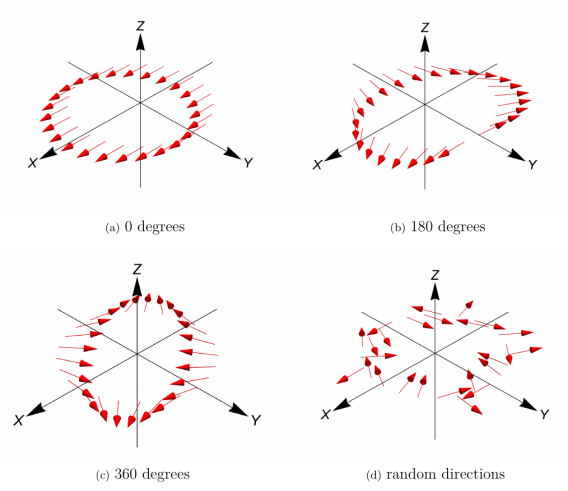
Figure 1: Visualization of the four initial product states studied in this work. The arrows correspond to the single-spin expectation values, see text and Eq. (10). We will refer to this states as $\ket{\psi_{A}}$, $\ket{\psi_{B}}$, $\ket{\psi_{C}}$, and $\ket{\psi_{D}}$.

In a product state, the spins are not entangled by definition, however they entangle during the unitary time evolution

$$\ket{\psi(t)}=e^{-\mathrm{i}\!\hbox{}\mathop{\vphantom{H}\smash{H}}\limits_{\sim}\hbox{}\!t}\ket{\psi(0)}\ ,$$ (12)

that we calculate numerically exactly using a Suzuki Trotter decomposition [34].

In order to measure the entanglement of an individual spin at site $j$ with the others, we define the reduced density matrix

$$\!\hbox{}\mathop{\vphantom{\rho}\smash{\rho}}\limits_{\sim}\!{}_{j}=\textsl{Tr}_{\bigotimes\limits_{k\neq j}\mathscr{H}_{k}}\left(\ket{\psi}\bra{\psi}\right)\ .$$ (13)

Here $\mathscr{H}_{j}$ denotes the Hilbert subspace of spin $j$, and $\mathscr{H}=\bigotimes\limits_{j=1}^{N}\mathscr{H}_{j}$ is the total Hilbert space. The purity is given as $\textsl{Tr}\left(\!\hbox{}\mathop{\vphantom{\rho}\smash{\rho}}\limits_{\sim}\!{}_{j}^{2}\right)$. $\textsl{Tr}\left(\!\hbox{}\mathop{\vphantom{\rho}\smash{\rho}}\limits_{\sim}\!{}_{j}^{2}\right)=1$ holds, if spin $j$ is not entangled with other spins, and $\textsl{Tr}\left(\!\hbox{}\mathop{\vphantom{\rho}\smash{\rho}}\limits_{\sim}\!{}_{j}^{2}\right)=0.5$ if it is maximally entangled with other spins. The purity is thus also a measure of decoherence for an observer of a single spin [35, 36]. An alternative way of quantifying the decoherence would be the von Neumann entropy $S(\!\hbox{}\mathop{\vphantom{\rho}\smash{\rho}}\limits_{\sim}\!{}_{j})=-\textsl{Tr}\left(\!\hbox{}\mathop{\vphantom{\rho}\smash{\rho}}\limits_{\sim}\!{}_{j}\log_{2}\!\hbox{}\mathop{\vphantom{\rho}\smash{\rho}}\limits_{\sim}\!{}_{j}\right)$ [37].

III Calculations and results

In this Section we present our numerical findings of the special behaviour of initial states in Fig. 1 under time evolution with Hamiltonian Eq. (1) and equal magnetic fields $h_{j}=-1\;\forall j$. As discussed, $M_{\text{trans}}$ and $\vec{\!\hbox{}\mathop{\vphantom{S}\smash{S}}\limits_{\sim}\!{}^{2}}$ are conserved quantities. We show that, with one exception, the spin expectation values synchronize.

III.1 Initial state $\ket{\psi_{A}}$

In Fig. 2 we start with initial state $\ket{\psi_{A}}$ and random Heisenberg interactions $J_{j}$. In this case, every spin is precessing as if independent without entangling to other spins, no matter how the $J_{j}$ are chosen. Since all spins point in the same direction, $M_{\text{trans}}$ and $\vec{\!\hbox{}\mathop{\vphantom{S}\smash{S}}\limits_{\sim}\!{}^{2}}$ assume their maximum values. Because they are conserved quantities the spins are bound to remain in a perfect product state, otherwise it would not be possible to conserve these values over time.

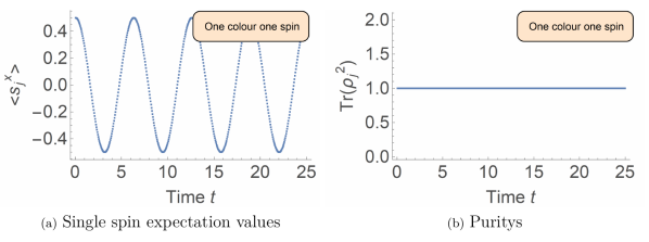
Figure 2: Time evolution of initial state $\ket{\psi_{A}}$ regarding Hamiltonian Eq. (1) with isotropic Heisenberg interactions and $J_{j}\in{[1.6,2.4]}$, $h_{j}=-1\;\forall j$, $N=25$. Left panel: Single-spin expectation values in $x$-direction. Right panel: Purity of the individual reduced density matrices.

III.2 Initial state $\ket{\psi_{B}}$

Figure 3 shows almost the same as Fig. 2, but this time for initial state $\ket{\psi_{B}}$. Initially the individual spin expectation values are spread out by $180$ degrees, but during time evolution they align. This astonishing phenomenon can be nicely observed in the video provided on the web page of the published article [30].

During time evolution and synchronization the spins entangle as much as the conservation of $\vec{\!\hbox{}\mathop{\vphantom{S}\smash{S}}\limits_{\sim}\hbox{}\!}^{2}$ and $M_{\text{trans}}$ allows. Interestingly, the spins stay entangled and do not fan out again (apart from finite size effects such as revivals at very late times). This statement becomes stronger with increasing system size, which is further addressed in Appendix A. We interpret this phenomenon as quantum mechanical equlibration process under the restricting influence of conserved quantities [29].

The synchronization can be rationalized for spin systems where all spins are equivalent, i.e. ring systems with translational invariance ($J_{j}=J$, $h_{j}=h\;\forall j$) since then equilibration should result in the same single-spin expectation value at every site. This concerns magnitude and direction of the spin vector. The somewhat unexpected result of our investigation is that the direction of all spins continues to synchronize also for settings where spins are no longer equivalent, i.e. if the Heisenberg interactions are drawn at random from a distribution.

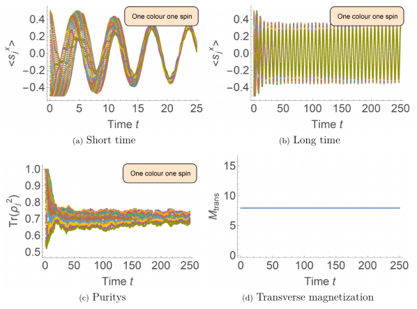
Figure 3: Time evolution of initial state $\ket{\psi_{B}}$ w.r.t. Hamiltonian Eq. (1) with isotropic Heisenberg interactions and $J_{j}\in{[1.6,2.4]}$, $h_{j}=-1\;\forall j$, $N=25$. The video for 3(a) can be found at [30].

Figure 3(c) shows the purity of the individual reduced density operators $\!\hbox{}\mathop{\vphantom{\rho}\smash{\rho}}\limits_{\sim}\!{}_{j}$ (Eq. (13)). Since the couplings $J_{j}$ are different for different $j$, not all spins are equal. This does not prevent the spins from synchronizing their directions, but they do not all entangle to the same extent.

Another main result of this paper is that the time needed for the spins to synchronize is almost independent of the width $\Delta$ of the distribution of the $J_{j}\in{[2-\Delta,2+\Delta]}$. This is also demonstrated numerically in Appendix A.

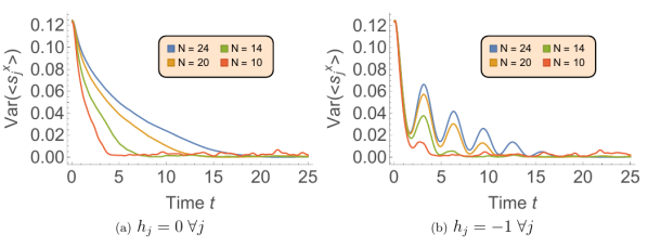
Figure 4: Time evolution of initial state $\ket{\psi_{B}}$ w.r.t. Hamiltonian Eq. (1) with isotropic Heisenberg interactions and $J_{j}=2\;\forall j$ without (a) and with magnetic field (b).

Figure 4 shows the variance of the expectation values of individual spin operators, defined as

$$\textsf{Var}(<\!\hbox{}\mathop{\vphantom{s}\smash{s}}\limits_{\sim}\!{}_{j}^{x}>)(t):=\frac{1}{N}\sum_{j=1}^{N}\left(<\!\hbox{}\mathop{\vphantom{s}\smash{s}}\limits_{\sim}\!{}_{j}^{x}>-\frac{<S^{x}>}{N}\right)^{2}$$ (14)

for different system sizes $N$. That the variance decays to zero, compare Fig. 4, expresses precisely that the spins align until they point in the same direction. This process takes the longer the larger the system is. The synchronisation, i.e. the alignment of directions, also takes place in the absence of a magnetic field, as can be seen in Fig. 4(a). The reason is that the homogeneous magnetic field, which is a one-body operator, does not causes any many-body entanglement between the spins; entanglement and equilibration are driven by the Heisenberg term which is a two-body operator. As a result, the field-free curves in Fig. 4(a) are the envelopes of the curves taken with homogeneous field and shown in Fig. 4(b).

III.3 Initial state $\ket{\psi_{C}}$

Figure 5 shows the time evolution for initial state $\ket{\psi_{C}}$ and different system sizes. This is a very special and atypical case with a particular symmetry in the spin orientations which results in a very stable state even if there are different couplings $J_{j}$ between the spins, see video [30]. This is the only initial state we find where the spins do not align, but entangle and decay to zero, with wild echos at later times. The larger the system, the longer the echos take to occur and the longer it takes for the spins to entangle.

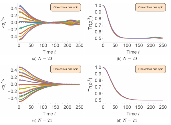
Figure 5: Time evolution of initial state $\ket{\psi_{C}}$ w.r.t. Hamiltonian Eq. (1) with isotropic Heisenberg interactions and $J_{j}\in{[1.6,2.4]}$, $h_{j}=0\;\forall j$ for different system sizes. The video of 5(c) is provided at [30].

These numerical results for finite system sizes suggest that $\ket{\psi_{C}}$ is an energy eigenstate in the thermodynamic limit which appears plausible, because the angle between neighboring spins is given by $2\pi/N$, therefore for $N\rightarrow\infty$ all neighbors are parallel in the initial state. We emphasize that this state would also be an energy eigenstate in the non-integrable case [38, 39] where the $J_{j}$ are all different. Because all single-spin observables are strongly different we conjecture that this state is not thermal; its relation to quantum scars needs to be explored, see [40, 41] and references therein.

III.4 Initial state $\ket{\psi_{D}}$

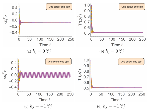
Figure 6: Time evolution of initial state $\ket{\psi_{D}}$ w.r.t. Hamiltonian Eq. (1) with isotropic Heisenberg interactions and $J_{j}\in{[1.6,2.4]}$, $N=24$ without (a-b) and with magnetic field (c-d). Video 6(c) is provided at [30].

Figure 6 shows a time evolution for initial state $\ket{\psi_{D}}$ (random orientations) without magnetic field (Fig. 6(a)) and with magnetic field (Fig. 6(b)). The conserved net magnetization is small (would be zero in the thermodynamic limit or as a mean of many random realizations according to the central limit theorem). Nevertheless, the spins synchronize which shows that this phenomenon is very robust with respect to the initial state, see also video [30].

III.5 Classical spin dynamics

Although not at the heart of our investigations, we like to compare our results to classical spin dynamics with identical Heisenberg couplings and initial states. It turns out that a classical spin dynamics does not exhibit phase synchronization, see videos [30]. The reason in this context is that classical spin dynamics lacks entanglement which is necessary for synchronization. Contrary to the expectation values of the quantum spins, the classical spins are bound to maintain their length, which effectively acts like additional $N$ conservation laws. This results in a oscillatory dynamics of most investigated initial conditions, compare Fig. 7 for initial states equivalent to Fig. 2(b)-(d). Initial state C is again special. In the quantum case the spins maintain their directions for a long time while slowly entangling. In the classical case the spins also keep their directions for a long time. This is because of the high symmetry in the initial state with zero net magnetization and no preferred direction in the $x$y-plane.

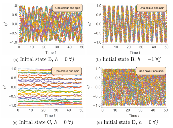
Figure 7: Classical time evolution for various initial states w.r.t. Hamiltonian Eq. (15) with $N=24$, $J_{j}\in{[1.6,2.4]}$. Videos for all cases are provided at [30].

The classical spin dynamics has been evaluated according to

$$\frac{d}{dt}\vec{s}_{j}=\frac{\partial H}{\partial\vec{s}_{j}}\times\vec{s}_{j}\ ,$$ (15)

where $H$ denotes the classical Hamiltonian analogous to Eq. (1).

In the literature one finds well-studied classical examples of synchronization of e.g. Van der Pol oscillators [42]. These are dissipative systems with stable limit cycles, which means that after a perturbation they return to their ordinary oscillation. This would not be the case for our classical spins even if we would couple them to a heat bath.

One trivial (but much different) way of how our classical spins would synchronize (at least in a transient way) is by choosing a ferromagnetic Heisenberg coupling $J_{j}$ and a dissipative dynamics so that the ferromagnetic ground state is approached which is aligned trivially.

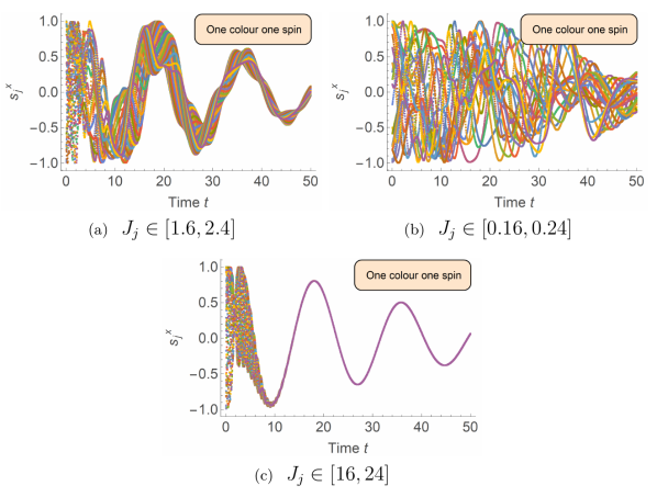
Figure 8: Damped classical time evolution for initial state B w.r.t. Hamiltonian Eq. (16), $\alpha=0.1$, $N=24$, $h_{j}=-1\;\forall j$ and different intervals of the ferromagnetic coupling strength.

Figure 8 shows such an example for different intervals of the Heisenberg coupling strength. The damping is realized by

$$\frac{d}{dt}\vec{s}_{j}=\frac{\partial H}{\partial\vec{s}_{j}}\times\vec{s}_{j}-\alpha\left(\frac{\partial H}{\partial\vec{s}_{j}}\times\vec{s}_{j}\right)\times\vec{s}_{j}\ .$$ (16)

Because of the damping, the system looses energy until it arrives in the lowest possible energy state. Since a ferromagnetic coupling is chosen, the spins synchronize per default. In Fig. 8 there is also a magnetic field applied in $z$-direction with which the spins also align. Therefore, at late times all spins point in $z$-direction. If the ferromagnetic coupling is much larger than the magnetic field $|J_{j}|\gg|h|$, then also the $x$- and $y$-components of the spins synchronize in a transient way.

We note that such kind of synchronization is fundamentally different from the synchronization we observe in closed quantum spin systems. In the quantum case, it does not matter if the Heisenberg interaction is ferro- or antiferromagnetic. The synchronization is just based on equilibration, entanglement, and conservation laws.

IV Breaking the symmetry

In this Section we investigate whether synchronization still occurs if $M_{\text{trans}}$ and $\vec{\!\hbox{}\mathop{\vphantom{S}\smash{S}}\limits_{\sim}\hbox{}\!}^{2}$ are not conserved anymore. We can break the symmetry in different ways, either by means of inhomogeneous magnetic fields or by interactions between the spins that are not of isotropic Heisenberg type. In Section (IV.1) we choose XYZ interactions and in Section (IV.2) XX interactions as two examples with different outcomes. In Appendix B we show the effect of inhomogeneous magnetic fields (App. B.1) and of dipolar interactions between all spins (App. B.2).

IV.1 XYZ interaction

We begin with the XYZ interaction which is close to the isotropic Heisenberg case if the interaction in the three spatial directions is not too different. In this case, the synchronization between the spins still occurs. The Hamiltonian in this subsection is defined as

$$\!\hbox{}\mathop{\vphantom{H}\smash{H}}\limits_{\sim}\!{}_{XYZ}= -J\sum_{j=1}^{N}\!\hbox{}\mathop{\vphantom{s}\smash{s}}\limits_{\sim}\!{}_{j}^{x}\!\hbox{}\mathop{\vphantom{s}\smash{s}}\limits_{\sim}\!{}_{j+1}^{x}-(J-\delta)\sum_{j=1}^{N}\!\hbox{}\mathop{\vphantom{s}\smash{s}}\limits_{\sim}\!{}_{j}^{y}\!\hbox{}\mathop{\vphantom{s}\smash{s}}\limits_{\sim}\!{}_{j+1}^{y}$$

$$-(J-2\delta)\sum_{j=1}^{N}\!\hbox{}\mathop{\vphantom{s}\smash{s}}\limits_{\sim}\!{}_{j}^{z}\!\hbox{}\mathop{\vphantom{s}\smash{s}}\limits_{\sim}\!{}_{j+1}^{z}-h\sum_{j=1}^{N}\!\hbox{}\mathop{\vphantom{s}\smash{s}}\limits_{\sim}\!{}_{j}^{z}\;.$$ (17)

We use the parameter $\delta$ to tune the difference of the interaction in the three spatial directions.

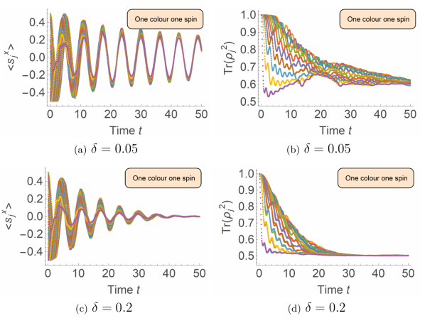
Figure 9: Time evolutions of initial state $\ket{\psi_{B}}$ w.r.t. Hamiltonian Eq. (17) for two values of $\delta$, and $N=24$, $J=2$, $h=-1$. Videos of 9(a) and (c) are provided at [30].

Figure 9 shows time evolutions for initial state $\ket{\psi_{B}}$ and two different values of $\delta$. The magnetization is not a conserved quantity anymore and will therefore decay towards its equilibrium value, which is zero in the $xy$-plane for a magnetic field in $z$-direction. Our investigations reveal that the larger $\delta$ the faster the spins decay. However, we clearly observe that while decaying the spins still synchronize, see especially Fig. 9(a). One could say, that the synchronization is a transient phenomenon in such cases since the time scale of synchronization is shorter than that of the unavoidable decay.

Fugure 9(b) and Fig. 9(d) show the purity of the reduced density operators $\!\hbox{}\mathop{\vphantom{\rho}\smash{\rho}}\limits_{\sim}\!{}_{j}$ introduced in Eq. (13).We see that all spins maximally entangle ($\textsl{Tr}\left(\!\hbox{}\mathop{\vphantom{\rho}\smash{\rho}}\limits_{\sim}\!{}_{j}^{2}\right)=0.5$) which is equivalent with all individual spin expectation values decay to zero.

Another example of broken symmetry where the spins still synchronize is shown in Appendix B.1 with an inhomogeneous magnetic field.

IV.2 XX interaction

As comparison we now show a case with XX interaction where the spins do not synchronize. The Hamiltonian is defined as

$$\!\hbox{}\mathop{\vphantom{H}\smash{H}}\limits_{\sim}\!{}_{XX}= -J\sum_{j=1}^{N}\left(\!\hbox{}\mathop{\vphantom{s}\smash{s}}\limits_{\sim}\!{}_{j}^{x}\!\hbox{}\mathop{\vphantom{s}\smash{s}}\limits_{\sim}\!{}_{j+1}^{x}+\!\hbox{}\mathop{\vphantom{s}\smash{s}}\limits_{\sim}\!{}_{j}^{y}\!\hbox{}\mathop{\vphantom{s}\smash{s}}\limits_{\sim}\!{}_{j+1}^{y}\right)-h\sum_{j=1}^{N}\!\hbox{}\mathop{\vphantom{s}\smash{s}}\limits_{\sim}\!{}_{j}^{z}\;.$$ (18)

Figure 10 shows a time evolution for initial state $\ket{\psi_{B}}$. The decay of the transverse magnetization is much faster than in the previous subsection, because we are further away from isotropic Heisenberg interactions and the symmetry regarding the conservation of the transverse magnetization is broken much more strongly, compare also [17]. In order to see if the spins still synchronize while decaying to zero, we choose a much smaller coupling constant $J=0.1$ instead $J=2$. But we clearly see that the spins do not synchronize while decaying or equivalently the timescale of the decay is much higher than the timescale of synchronization.

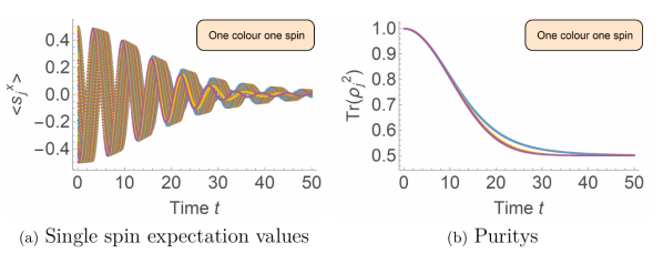
Figure 10: Time evolution of initial state $\ket{\psi_{B}}$ w.r.t. Hamiltonian Eq. (18) with parameters $N=24$, $J=0.1$ and $h=-1$. The video of 10(a) can be found at [30].

Another example of broken symmetry where the spins do not synchronize is shown in Appendix B.2 with dipolar interactions between the spins.

In a future investigation, we plan to study the relation of our findings for the translationally invariant XXZ case with the suggestion of a generalized Gibbs ensemble as the long-time limit of the unitary dynamics induced by dynamical symmetries according to Refs. [43, 44, 45].

V Summary

As a conclusion we can say first of all that the conservation of $M_{\text{trans}}$ and $\vec{\!\hbox{}\mathop{\vphantom{S}\smash{S}}\limits_{\sim}\hbox{}\!}^{2}$ not just slows down the FID, but prevents the free induction from decaying if the Hamiltonian only contains isotropic Heisenberg interactions and the Zeeman terms of all spins are equal (see Fig. 2). This is in accord with Ref. [29].

Furthermore, we demonstrate in detail the interesting phenomenon that the single-spin vector expectation values align in the course of time almost independent of how they are initialized in the $xy$-plane (see Fig. 3). It does not matter if the initial state is a product state of the form Eq. (10) or if the spins start in an entangled state (see Appendix A.3). For the process of synchronization the magnetic field is not necessary, it only induces a (collective) rotation of all spins about the field axis (see e.g. Fig. 4 and Fig. 11). The Heisenberg interactions cause an equilibration process under the constraint of conserved quantities. We show that after entanglement is maximised (under constraints of conserved quantities) and equilibration is completed the spins stay synchronized and fluctuate the less the larger the system is (see e.g. Fig. 14, Apppendix A.1). Moreover, we show that the timescale of synchronization is independent of the width $\Delta$ of the variation of Heisenberg couplings $J_{j}$ (see Fig. 15, Apppendix A.1).

We demonstrate that such a synchronization is not possible with classical spins in a closed system (see Fig. 7). Moreover we give an example for dissipative classical spins which experience a transient synchronization based on ferromagnetism (see Fig. 8). We highlight that this is very different from the observed quantum mechanical synchronization where the system is closed and the sign of the Heisenberg interaction does not matter.

In addition, we discuss that the synchronization of spin expectation values is very robust. It happens already for small systems ($N=10$, see Fig. 13, Apppendix A) and for various initial states (see e.g. Fig. 6). We find just one exception (initial state $\ket{\psi_{C}}$) which has a special symmetry and in the thermodynamic limit becomes an energy eigenstate (see Fig. 5). Synchronization also occurs for long-range Heisenberg interactions (see Fig. 21, Appendix B.2). Synchronization is not limited to spins $s=1/2$. In Appendix A.2 we demonstrate that also spins with $s=1$ synchronize under isotropic Heisenberg interactions.

Further on, we provide examples of transient synchronization for systems where symmetries are broken, because the time scale of synchronization is shorter than that of equilibration. Systems with anisotropic XYZ interactions belong to this set if they are still close to the isotropic Heisenberg case (see Fig. 9), or if the symmetry is broken by means of an inhomogeneous magnetic field (see Fig. 18 and Apppendix B.1, respectively).

Finally, we show that spins do not synchronize for interactions that are strongly anisotropic such as dipolar interactions (see Fig. 20, Appendix B.2).

Our investigations might be helpful for interpreting observations in the context of FID. Even if we cannot provide a complete analytical explanation of the phenomenon, we think the wide range of numerical results demonstrates that the phenomenon of synchronization is widespread and robust.

Appendix A Additions to section III

A.1 More data regarding section III.2

Here we present more detailed numerical calculations regarding Section III.2. In Fig. 11 the purity of individual reduced density matrices is shown for different system sizes $N$. All Heisenberg couplings $J_{j}$ are chosen equal and therefore all spins entangle in an equal way during equilibration (in contrast to Fig. 3(c)).

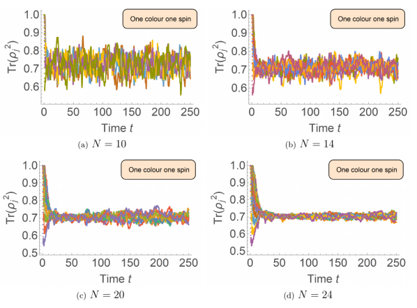
Figure 11: Purities of the time evolution of initial state $\ket{\psi_{B}}$ w.r.t. Hamiltonian Eq. (1) with isotropic Heisenberg interactions and $J_{j}=2\;\forall j$, $h_{j}\equiv h\;\forall j$. The value of $h$ does not change this figure.

It can be clearly seen that the respective purities fluctuate less the larger the system is. Thus, in the thermodynamic limit ($N\rightarrow\infty$) we expect them to keep the same order of magnitude without fluctuating after equilibration. This figure is completely independent of the strength of the magnetic field $h$, because the Zeeman term in Hamiltonian Eq. (1) does not cause any entanglement between spins.

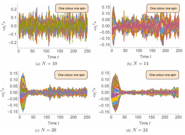
Figure 12: Single spin expectation values in $z$-direction regarding time evolution of initial state $\ket{\psi_{B}}$ w.r.t. Hamiltonian Eq. (1) with isotropic Heisenberg interactions and $J_{j}=2\;\forall j$, $h_{j}\equiv-1\;\forall j$.

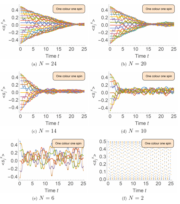
Figure 13: Single spin expectation values in $x$-direction regarding time evolution of initial state $\ket{\psi_{B}}$ w.r.t. Hamiltonian Eq. (1) with isotropic Heisenberg interactions and $J_{j}=2\;\forall j$, $h_{j}=0\;\forall j$ for various system sizes (short time).

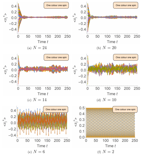
Figure 14: Same as Fig. 13, but long time.

Figure 12 shows the individual $\langle s_{j}^{z}\rangle$ expectation values for exactly the same time evolutions as Fig. 11. Initially all these values are zero because the spins are oriented in the $xy$-plane (see Fig. 1). During time evolution (especially at the beginning) the spins leave the $xy$-plane, but at later times these fluctuations in $z$-direction become small for a larger system size $N$.

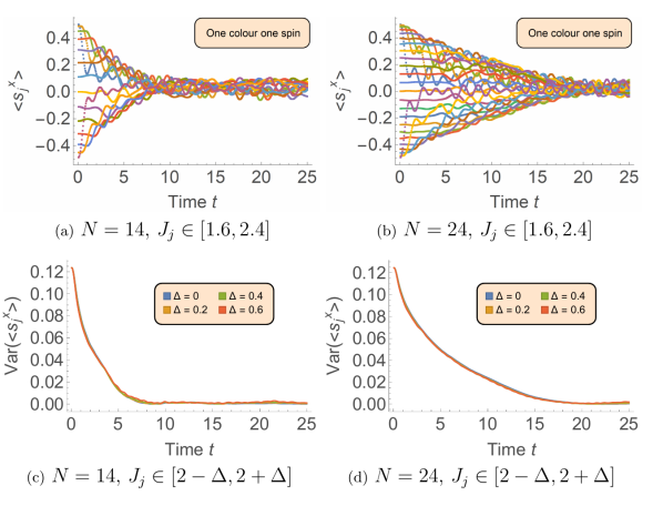
Figure 15: Time evolution of initial state $\ket{\psi_{B}}$ w.r.t. Hamiltonian Eq. (1) with isotropic Heisenberg interactions from intervals of different width $\Delta$, $J_{j}\in{[2-\Delta,2+\Delta]}$ and different system sizes $N$, $h_{j}=0\;\forall j$.

Figure 13 and Fig. 14 show individual spin expectation values for time evolutions without magnetic field for different system sizes and for short and long time (also for initial state $\ket{\psi_{B}}$). It can be qualitatively seen that such synchronization of spins can already be observed for a small system size of $N=10$. For $N=6$ the spins fluctuate much and for $N=2$ the spins permanently point in opposite directions.

We now want to focus on the question how the choice of couplings $J_{j}$ influences the time needed for the spins to align. This is addressed by Fig. 15. The couplings $J_{j}$ are chosen randomly from intervals of different width $\Delta$ and the magnetic field is zero. We see that $\Delta$ has a very small impact on the time evolution and the behaviour of the spins; the process of alignment and the time it takes is very robust. The time to synchronization does only depend on the system size $N$ and the mean $J_{j}$.

A.2 Spins $\zeta=1$

The question arises if the observed synchronization phenomenon also occurs with larger spins than $s=1/2$. To address this question at least partly, we simulate spin rings with spin quantum numbers $\zeta=1$. To simplify our numerical calculation we form these spins by coupling two spins with $s=1/2$ each ferromagnetically. We define

$$\vec{\!\hbox{}\mathop{\vphantom{\zeta}\smash{\zeta}}\limits_{\sim}\hbox{}\!}_{j}:=\vec{\!\hbox{}\mathop{\vphantom{s}\smash{s}}\limits_{\sim}\hbox{}\!}_{2j}+\vec{\!\hbox{}\mathop{\vphantom{s}\smash{s}}\limits_{\sim}\hbox{}\!}_{2j-1}\ .$$ (19)

Instead of $N$ spins with $s=1/2$ we have $\tilde{N}=N/2$ spins with $\zeta=1$. The following Hamiltonian applies

$$\!\hbox{}\mathop{\vphantom{H}\smash{H}}\limits_{\sim}\hbox{}\!=-\sum_{j=1}^{\tilde{N}}J_{j}\vec{\!\hbox{}\mathop{\vphantom{\zeta}\smash{\zeta}}\limits_{\sim}\hbox{}\!}_{j}\cdot\vec{\!\hbox{}\mathop{\vphantom{\zeta}\smash{\zeta}}\limits_{\sim}\hbox{}\!}_{j+1}-\sum_{j=1}^{N}h_{j}\!\hbox{}\mathop{\vphantom{\zeta}\smash{\zeta}}\limits_{\sim}\!{}_{j}^{z}$$

$$-J_{f}\sum_{j=1}^{\tilde{N}}\vec{\!\hbox{}\mathop{\vphantom{s}\smash{s}}\limits_{\sim}\hbox{}\!}_{2j}\cdot\vec{\!\hbox{}\mathop{\vphantom{s}\smash{s}}\limits_{\sim}\hbox{}\!}_{2j-1}\ ,$$ (20)

The last term in Eq. (20) is the strong ferromagnetic coupling, $J_{f}=100\gg|J_{j}|$, between every two fused spins. We initialize the state of the system such that those two coupled spins point in the same direction and the $\tilde{N}$ spins are fanned out by $180$ degrees. The time evolution is shown in Fig. 16, and indeed the spins still synchronize.

We thus speculate that there is no obvious or simple classical limit by which synchronizations would disappear when going from small spin quantum numbers to large spin quantum numbers. Also the time scale on which synchronization happens does not seem to be very different between spins $s=1/2$ and $\zeta=1$, compare Figs. 16(a) and 13(d). This question certainly needs further investigations.

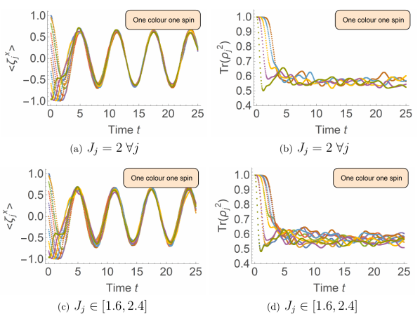
Figure 16: Time evolution of initial state $\ket{\psi_{B}}$ w.r.t. Hamiltonian Eq. (1) with $h_{j}=-1\;\forall j$, $\tilde{N}=10$ spins with $\zeta=1$ (technically realized as fused pairs of spins with $s=1/2$ each).

A.3 Starting in an entangled state

So far our initial state was always a product state Eq. (10). That might give the impression that this could be relevant for the phenomenon of synchronization. But this is not the case, as we show with one example in this subsection.

Consider the state

$$\ket{\phi}=\sum_{k=1}^{N}c_{k}\ket{k}\ ,$$ (21)

with Gaussian distributed random coefficients and an arbitrary basis $\ket{k}$ of the Hilbert space. Such a state will be maximally entangled and all spin expectation values are close to zero. From this we construct our initial state

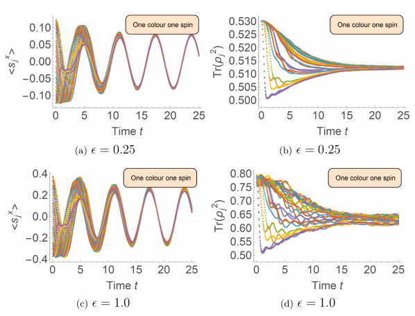
Figure 17: Time evolution of initial state Eq. (22) w.r.t. Hamiltonian Eq. (1) with isotropic Heisenberg interactions and $J_{j}\in{[1.6,2.4]}$, $h_{j}=-1\;\forall j$, $N=24$ and two different values of $\epsilon$.

$$\ket{\psi}\propto\left(\prod_{j=1}^{N}e^{\epsilon\sin{(\alpha_{j})}\!\hbox{}\mathop{\vphantom{s}\smash{s}}\limits_{\sim}\!{}_{j}^{x}}e^{\epsilon\sin{(\alpha_{j})}\!\hbox{}\mathop{\vphantom{s}\smash{s}}\limits_{\sim}\!{}_{j}^{y}}\right)\ket{\phi}\ ,$$ (22)

with $\alpha_{j}=\frac{j\pi}{N}$ and $\epsilon$ a parameter for the magnitude of the deflection of the spin expectation values from zero. This way we create a (still entangled) state with single spin expectations values $\neq 0$ in the xy-plane fanned out by $180$ degrees. Fig. 17 shows associated time evolutions and that the spins do indeed still synchronize, starting in an entangled state Eq. (22).

Appendix B Additions to section IV

In addition to sec. IV we present more cases of how the spins behave with broken symmetry (without the conserved quantities $M_{\text{trans}}$ and $\vec{\!\hbox{}\mathop{\vphantom{S}\smash{S}}\limits_{\sim}\!{}^{2}}$).

B.1 Inhomogeneous magnetic field

As shown in Eq. (3) all magnetic fields $h_{j}$ have to be equal or the conserved quantities are broken.

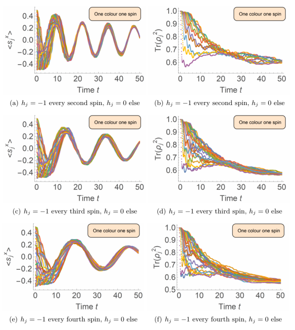
Figure 18: Time evolution of initial state $\ket{\psi_{B}}$ w.r.t. Hamiltonian Eq. (1) with isotropic Heisenberg interactions and $J_{j}=2\;\forall j$, $N=24$ and for different configurations of $h_{j}$. Videos of 18(a) and (e) are provided at [30].

Figure 18 shows time evolutions of initial state $\ket{\psi_{B}}$ where only a few spins see a magnetic field $h_{j}=h\neq 0$ and all others fields are zero. Surprisingly the spins do still synchronize an precess together while they decay. The spins without magnetic field are carried with the others.

The frequency $\tilde{h}$ of the collective precession decreases the more spins there are with $h_{j}=0$. This can be viewed as every spin sees a mean field $\tilde{h}=\sum_{j}h_{j}/N$. From Fig. 18(a) to Fig. 18(e) the number of magnetic fields $h_{j}=h$ is halved and the precession frequency $\tilde{h}$ also halves.

Another way of breaking the symmetry is by choosing random magnetic fields. Figure 19 shows time evolutions for initial state $\ket{\psi_{B}}$ where the magnetic fields $h_{j}$ are drawn at random from a distribution of different width $\xi$. The spins do still synchronize up to large values of $\xi$ up to the point where the decay of the transverse magnetization is faster than the synchronization.

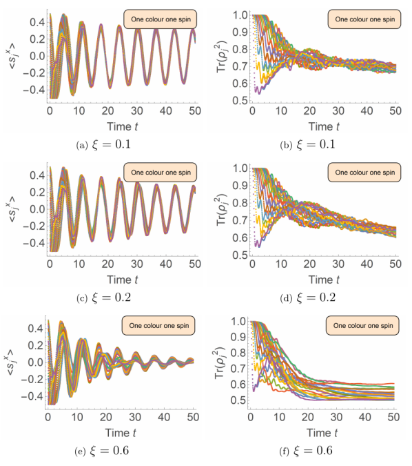
Figure 19: Time evolution of initial state $\ket{\psi_{B}}$ w.r.t. Hamiltonian Eq. (1) with isotropic Heisenberg interactions, $J_{j}=2\;\forall j$, $N=24$ and $h_{j}\in{[-1-\xi,-1+\xi]}$. Videos of 19(a) and (e) are provided at [30].

B.2 Dipolar and long range interactions

We now investigate how initial state $\ket{\psi_{B}}$ behaves when all spins (not only neighbors) interact with dipolar interactions or just long-range Heisenberg interactions.

The Hamiltonian of a dipolar interacting spin system is given by

$$\!\hbox{}\mathop{\vphantom{H}\smash{H}}\limits_{\sim}\hbox{}\!= \sum_{j=1}^{N}\sum_{k=j+1}^{N}\frac{\lambda}{r_{jk}^{3}}\left(\!\hbox{}\mathop{\vphantom{\vec{s}}\smash{\vec{s}}}\limits_{\sim}\!{}_{j}\cdot\!\hbox{}\mathop{\vphantom{\vec{s}}\smash{\vec{s}}}\limits_{\sim}\!{}_{k}-\frac{3(\!\hbox{}\mathop{\vphantom{\vec{s}}\smash{\vec{s}}}\limits_{\sim}\!{}_{j}\cdot\vec{r}_{jk})(\!\hbox{}\mathop{\vphantom{\vec{s}}\smash{\vec{s}}}\limits_{\sim}\!{}_{k}\cdot\vec{r}_{jk})}{r_{jk}^{2}}\right)$$

$$-h\sum_{j=1}^{N}\!\hbox{}\mathop{\vphantom{s}\smash{s}}\limits_{\sim}\!{}_{j}^{z}\;.$$ (23)

We use the parameter $\lambda$ to tune the strength of the interaction. We also need spatial coordinates $\vec{r}_{j}$ for all spins. For simplicity we arrange them on the unit circle

$$\vec{r}_{j}=\left(\begin{array}[]{c}\cos(2\pi j/N)\\ \sin(2\pi j/N)\\ 0\end{array}\right)\;.$$ (27)

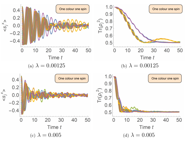
Figure 20: Time evolution of initial state $\ket{\psi_{B}}$ w.r.t. Hamiltonian Eq. (23) with coordinates Eq. (27), $N=24$, and for different parameters $\lambda$. The video of 20(a) can be found at [30].

Figure 20 shows time evolutions for initial state $\ket{\psi_{B}}$ for two different parameters $\lambda$. As expected the spin expectation values decay the faster the larger the parameter $\lambda$ is. But even for a small $\lambda$ in Fig. 20(a) the spins do not synchronize at all. This can also be seen in the related video at [30]. Dipolar interactions are highly anisotropic, therefore, the conservation of the transverse magnetization is broken strongly.

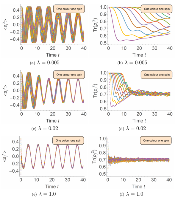
Figure 21: Time evolution of initial state $\ket{\psi_{B}}$ w.r.t. Hamiltonian Eq. (28) with coordinates Eq. (27), $N=24$, and for different parameters $\lambda$.

Finally, we want to test if synchronization under isotropic Heisenberg couplings is limited to nearest-neighbor interactions or holds under long-range interactions. To this end, we take as an example the above Hamiltonian Eq. (23) and remove the anisotropic parts

$$\!\hbox{}\mathop{\vphantom{H}\smash{H}}\limits_{\sim}\hbox{}\!=\sum_{j=1}^{N}\sum_{k=j+1}^{N}\frac{\lambda}{r_{jk}^{3}}\!\hbox{}\mathop{\vphantom{\vec{s}}\smash{\vec{s}}}\limits_{\sim}\!{}_{j}\cdot\!\hbox{}\mathop{\vphantom{\vec{s}}\smash{\vec{s}}}\limits_{\sim}\!{}_{k}-h\sum_{j=1}^{N}\!\hbox{}\mathop{\vphantom{s}\smash{s}}\limits_{\sim}\!{}_{j}^{z}\;.$$ (28)

Again we tune the interaction strength by the parameter $\lambda$. Fig. 21 shows calculations for very small to larger values of $\lambda$. For $\lambda=0.005$ in Fig. 21 the time scale shown is not sufficient for the spins to synchronize, whereas in Fig. 20(c) there is enough time for the magnetization to decay completely. This shows that the magnetization decay through the anisotropic terms of the dipolar interaction happens on a much faster time scale than the isotropic part causes synchronization. Choosing $\lambda$ significantly larger in Fig. 21 leads to synchronization in the given time frame.

One finding of this chapter is that the synchronization effect is more general, and it does not only appear for nearest-neighbor isotropic Heisenberg interactions.

References

- Deutsch [1991] J. M. Deutsch, Quantum statistical mechanics in a closed system, Phys. Rev. A 43, 2046 (1991).
- Srednicki [1994] M. Srednicki, Chaos and quantum thermalization, Phys. Rev. E 50, 888 (1994).
- Schnack and Feldmeier [1996] J. Schnack and H. Feldmeier, Statistical properties of fermionic molecular dynamics, Nucl. Phys. A 601, 181 (1996).
- Rigol et al. [2008] M. Rigol, V. Dunjko, and M. Olshanii, Thermalization and its mechanism for generic isolated quantum systems, Nature 452, 854 (2008).
- Polkovnikov et al. [2011] A. Polkovnikov, K. Sengupta, A. Silva, and M. Vengalattore, Colloquium: Nonequilibrium dynamics of closed interacting quantum systems, Rev. Mod. Phys. 83, 863 (2011).
- Reimann and Kastner [2012] P. Reimann and M. Kastner, Equilibration of isolated macroscopic quantum systems, New J. Phys. 14, 043020 (2012).
- Steinigeweg et al. [2014] R. Steinigeweg, A. Khodja, H. Niemeyer, C. Gogolin, and J. Gemmer, Pushing the limits of the eigenstate thermalization hypothesis towards mesoscopic quantum systems, Phys. Rev. Lett. 112, 130403 (2014).
- Gogolin and Eisert [2016] C. Gogolin and J. Eisert, Equilibration, thermalisation, and the emergence of statistical mechanics in closed quantum systems, Rep. Prog. Phys. 79, 056001 (2016).
- D’Alessio et al. [2016] L. D’Alessio, Y. Kafri, A. Polkovnikov, and M. Rigol, From quantum chaos and eigenstate thermalization to statistical mechanics and thermodynamics, Adv. Phys. 65, 239 (2016).
- Borgonovi et al. [2016] F. Borgonovi, F. M. Izrailev, L. F. Santos, and V. G. Zelevinsky, Quantum chaos and thermalization in isolated systems of interacting particles, Phys. Rep. 626, 1 (2016).
- Wu et al. [2017] Y.-L. Wu, D.-L. Deng, X. Li, and S. Das Sarma, Intrinsic decoherence in isolated quantum systems, Phys. Rev. B 95, 014202 (2017).
- Vorndamme and Schnack [2020] P. Vorndamme and J. Schnack, Decoherence of a singlet-triplet superposition state under dipolar interactions of an uncorrelated environment, Phys. Rev. B 101, 075101 (2020).
- Crooker et al. [1997] S. A. Crooker, D. D. Awschalom, J. J. Baumberg, F. Flack, and N. Samarth, Optical spin resonance and transverse spin relaxation in magnetic semiconductor quantum wells, Phys. Rev. B 56, 7574 (1997).
- Mizuochi et al. [2009] N. Mizuochi, P. Neumann, F. Rempp, J. Beck, V. Jacques, P. Siyushev, K. Nakamura, D. J. Twitchen, H. Watanabe, S. Yamasaki, F. Jelezko, and J. Wrachtrup, Coherence of single spins coupled to a nuclear spin bath of varying density, Phys. Rev. B 80, 041201 (2009).
- Cywiński et al. [2009] Ł. Cywiński, W. M. Witzel, and S. D. Sarma, Electron spin dephasing due to hyperfine interactions with a nuclear spin bath, Physical Review Letters 102, 057601 (2009).
- Ardavan et al. [2007] A. Ardavan, O. Rival, J. J. L. Morton, S. J. Blundell, A. M. Tyryshkin, G. A. Timco, and R. E. P. Winpenny, Will spin-relaxation times in molecular magnets permit quantum information processing?, Phys. Rev. Lett. 98, 057201 (2007).
- Jepsen et al. [2021] P. N. Jepsen, W. W. Ho, J. Amato-Grill, I. Dimitrova, E. Demler, and W. Ketterle, Transverse spin dynamics in the anisotropic Heisenberg model realized with ultracold atoms, (2021), arXiv:2103.07866 [cond-mat.quant-gas] .
- Balz and Reimann [2017] B. N. Balz and P. Reimann, Typical relaxation of isolated many-body systems which do not thermalize, Phys. Rev. Lett. 118, 190601 (2017).
- Weiss et al. [1992] S. Weiss, M.-A. Mycek, J.-Y. Bigot, S. Schmitt-Rink, and D. S. Chemla, Collective effects in excitonic free induction decay: Do semiconductors and atoms emit coherent light in different ways?, Phys. Rev. Lett. 69, 2685 (1992).
- Orth et al. [2010] P. P. Orth, D. Roosen, W. Hofstetter, and K. Le Hur, Dynamics, synchronization, and quantum phase transitions of two dissipative spins, Phys. Rev. B 82, 144423 (2010).
- Giorgi et al. [2013] G. L. Giorgi, F. Plastina, G. Francica, and R. Zambrini, Spontaneous synchronization and quantum correlation dynamics of open spin systems, Phys. Rev. A 88, 042115 (2013).
- Cabot et al. [2019] A. Cabot, G. L. Giorgi, F. Galve, and R. Zambrini, Quantum synchronization in dimer atomic lattices, Phys. Rev. Lett. 123, 023604 (2019).
- Karpat et al. [2020] G. Karpat, i. d. I. Yalç ınkaya, and B. Çakmak, Quantum synchronization of few-body systems under collective dissipation, Phys. Rev. A 101, 042121 (2020).
- Zhu et al. [2015] B. Zhu, J. Schachenmayer, M. Xu, F. Herrera, J. G. Restrepo, M. J. Holland, and A. M. Rey, Synchronization of interacting quantum dipoles, New Journal of Physics 17, 083063 (2015).
- Roulet and Bruder [2018] A. Roulet and C. Bruder, Synchronizing the smallest possible system, Phys. Rev. Lett. 121, 053601 (2018).
- Parra-López and Bergli [2020] A. Parra-López and J. Bergli, Synchronization in two-level quantum systems, Phys. Rev. A 101, 062104 (2020).
- Giorgi et al. [2019] G. L. Giorgi, A. Cabot, and R. Zambrini, Transient synchronization in open quantum systems, in Adv. in Open Systems and Fund. Tests of QM, edited by B. Vacchini, H.-P. Breuer, and A. Bassi (Springer International Publishing, Cham, 2019) pp. 73–89.
- Schnalle and Schnack [2010] R. Schnalle and J. Schnack, Calculating the energy spectra of magnetic molecules: application of real- and spin-space symmetries, Int. Rev. Phys. Chem. 29, 403 (2010).
- Uhrig et al. [2014] G. S. Uhrig, J. Hackmann, D. Stanek, J. Stolze, and F. B. Anders, Conservation laws protect dynamic spin correlations from decay: Limited role of integrability in the central spin model, Phys. Rev. B 90, 060301 (2014).
- [30] Videos are provided as supplementary material and at https://obelix.physik.uni-bielefeld.de/schnack/index-publications.html.
- Troiani et al. [2005] F. Troiani, A. Ghirri, M. Affronte, S. Carretta, P. Santini, G. Amoretti, S. Piligkos, G. Timco, and R. Winpenny, Molecular engineering of antiferromagnetic rings for quantum computation, Phys. Rev. Lett. 94, 207208 (2005).
- Ummethum et al. [2012] J. Ummethum, J. Nehrkorn, S. Mukherjee, N. B. Ivanov, S. Stuiber, T. Strässle, P. L. W. Tregenna-Piggott, H. Mutka, G. Christou, O. Waldmann, and J. Schnack, Discrete antiferromagnetic spin-wave excitations in the giant ferric wheel Fe18, Phys. Rev. B 86, 104403 (2012).
- Bärwinkel et al. [2000] K. Bärwinkel, H.-J. Schmidt, and J. Schnack, Structure and relevant dimension of the Heisenberg model and applications to spin rings, J. Magn. Magn. Mater. 212, 240 (2000).
- Hatano and Suzuki [2005] N. Hatano and M. Suzuki, Finding exponential product formulas of higher orders, in Quantum Annealing and Other Optimization Methods, edited by A. Das and B. K. Chakrabarti (Springer, Berlin, Heidelberg, 2005) pp. 37–68.
- Schlosshauer [2005] M. Schlosshauer, Decoherence, the measurement problem, and interpretations of quantum mechanics, Rev. Mod. Phys. 76, 1267 (2005).
- Schlosshauer [2014] M. Schlosshauer, The quantum-to-classical transition and decoherence, ArXiv e-prints (2014), arXiv:1404.2635 [quant-ph] .
- Donker et al. [2017] H. C. Donker, H. D. Raedt, and M. I. Katsnelson, Decoherence and pointer states in small antiferromagnets: A benchmark test, SciPost Phys. 2, 010 (2017).
- Babujian [1983] H. Babujian, Exact solution of the isotropic Heisenberg chain with arbitrary spins: Thermodynamics of the model, Nucl. Phys. B 215, 317 (1983).
- Frahm et al. [1990] H. Frahm, N.-C. Yu, and M. Fowler, The integrable XXZ Heisenberg model with arbitrary spin: Construction of the hamiltonian, the ground-state configuration and conformal properties, Nucl. Phys. B 336, 396 (1990).
- Choi et al. [2019] S. Choi, C. J. Turner, H. Pichler, W. W. Ho, A. A. Michailidis, Z. Papić, M. Serbyn, M. D. Lukin, and D. A. Abanin, Emergent SU(2) dynamics and perfect quantum many-body scars, Phys. Rev. Lett. 122, 220603 (2019).
- Pilatowsky-Cameo et al. [2021] S. Pilatowsky-Cameo, D. Villaseñor, M. A. Bastarrachea-Magnani, S. Lerma-Hernández, L. F. Santos, and J. G. Hirsch, Ubiquitous quantum scarring does not prevent ergodicity, Nat. Commun. 12, 852 (2021).
- van der Pol, Jr. [1926] B. van der Pol, Jr., LXXXVIII. On “relaxation-oscillations”, The London, Edinburgh, and Dublin Philosophical Magazine and Journal of Science 2, 978 (1926).
- Medenjak et al. [2020] M. Medenjak, B. Buča, and D. Jaksch, Isolated Heisenberg magnet as a quantum time crystal, Phys. Rev. B 102, 041117 (2020).
- Buča et al. [2019] B. Buča, J. Tindall, and D. Jaksch, Non-stationary coherent quantum many-body dynamics through dissipation, Nat. Commun. 10, 1730 (2019).
- Zadnik et al. [2016] L. Zadnik, M. Medenjak, and T. Prosen, Quasilocal conservation laws from semicyclic irreducible representations of Uq(sl2) in XXZ spin-1/2 chains, Nucl. Phys. B 902, 339 (2016).