Emergence of many-body quantum chaos via spontaneous breaking of unitarity
Supplemental Material

In this supplemental material, we present the detailed derivation for the spectral form factors of (1) a random matrix model with additional nonrandom two-body interactions (Sec. I); (2) a two-dimensional disordered system of fermions interacting via short-range density-density interactions (Sec. II).

I Random matrix model with interactions

In this section, we consider a system of $N\gg 1$ interacting fermions populating the single-particle energy levels of a Gaussian unitary ensemble, and is governed by the following Hamiltonian

$$\begin{aligned} H=\sum_{i,j=1}^{N}\psi^{\dagger}_{i}h_{ij}\psi_{j}+\frac{1}{2}\sum_{i,j,k,l=1}^{N}\psi^{\dagger}_{i}\psi^{\dagger}_{j}V_{ij;kl}\psi_{k}\psi_{l},\end{aligned}$$ (S1)

where $h$ is a $N\times N$ random Hermitian matrix drawn from a Gaussian unitary ensemble (GUE) with the distribution function

$$\begin{aligned} P(h)=\frac{1}{Z_{h}}\exp\left(-\frac{N}{2J^{2}}\operatorname{Tr}h^{2}\right),\qquad Z_{h}=\int\mathcal{D}h\exp\exp\left(-\frac{N}{2J^{2}}\operatorname{Tr}h^{2}\right).\end{aligned}$$ (S2)

The coupling $V$ of the two-body interactions is not random. We consider an arbitrary but fixed configuration of $V$ which is antisymmetrized:

$$\begin{aligned} V_{ij;kl}=-V_{ji;kl}=-V_{ij;lk}=V_{kl;ij}^{*}.\end{aligned}$$ (S3)

To investigate the spectral statistics of this model, we calculate the spectral form factor (SFF) defined as

$$\begin{aligned} K(\eta,t)=\,&\braket{Z(\eta+it)Z(\eta-it)}.\end{aligned}$$ (S4)

Here the angular bracket represents the ensemble averaging over random matrix $h$ with the weight $P(h)$ (Eq. S2), and $Z(\eta\pm it)=\operatorname{Tr}\left(e^{-(\eta\pm it)H}\right)$ is the analytically-continued partition function.

Without the interactions, the current model reduces to the $q=2$ complex Sachdev–Ye–Kitaev (SYK) model whose many-body level statistics has been investigated in Ref. Liao et al. (2020) (see also Ref. Winer et al. (2020) for a similar study of $q=2$ Majorana SYK model). Despite being integrable, the $q=2$ SYK model exhibits surprising rich structure which combines the single-particle chaotic and many-body integrable features, reflected by the exponential-in-$t$ ramp in its SFF. In the following, we show that, in the presence of interactions, $K(\eta\rightarrow 0^{+},t)\neq K(\eta=0,t)$. Furthermore, in the case of $\eta\rightarrow 0^{+}$, the soft modes responsible for the exponential ramp acquire a mass, leading to the suppression of the ramp.

I.1 Preliminaries

We start with a path integral formula for the spectral form factor:

$$\begin{aligned} K(\eta,t)=&\left\langle Z(iz_{+})Z(-iz_{-})\right\rangle\\ =&\left\langle\int\mathcal{D}(\bar{\psi},\psi)\exp\left\{i\sum_{a=\pm}\int_{0}^{z_{a}}dt^{\prime}\left[\bar{\psi}_{i}^{a}(t^{\prime})(i\partial_{t^{\prime}}\delta_{ij}-\zeta_{a}h_{ij})\psi_{j}^{a}(t^{\prime})-\frac{i}{2}\zeta_{a}\bar{\psi}_{i}^{a}(t^{\prime})\bar{\psi}_{j}^{a}(t^{\prime})V_{ij;kl}\psi_{k}^{a}(t^{\prime})\psi_{l}^{a}(t^{\prime})\right]\right\}\right\rangle,\end{aligned}$$ (S5)

where for simplicity we denote $t\mp i\eta$ by $z_{\pm}$. Besides the flavor index $i$, the Grassmann fields $\psi$ and $\bar{\psi}$ carry an additional replica index $a=\pm$. The path integral over $\psi^{a}$ and $\bar{\psi}^{a}$ is subject to the boundary condition:

$$\begin{aligned} \psi^{a}(z_{a})=-\psi^{a}(0),\qquad\bar{\psi}^{a}(z_{a})=-\bar{\psi}^{a}(0),\end{aligned}$$ (S6)

and gives rise to $Z(i\zeta_{a}z_{a})$. The sign factor $\zeta_{a}$ takes the value of $\pm 1$ for $a=\pm$

In the Fourier basis

$$\begin{aligned} \psi^{a}(\varepsilon_{n}^{a})=\frac{1}{z_{a}}\int_{0}^{z_{a}}dt^{\prime}\,\psi^{a}(t^{\prime})e^{i\varepsilon_{n}^{a}t^{\prime}},\qquad\varepsilon_{n}^{a}=\frac{2\pi}{z_{a}}(n+\frac{1}{2}),\end{aligned}$$ (S7)

Eq. S5 can be rewritten as

$$\begin{aligned} K(\eta,t)=&\left\langle\int\mathcal{D}(\bar{\psi},\psi)\exp\left\{\begin{aligned} &i\sum_{a,n}z_{a}\bar{\psi}_{i}^{a}(\varepsilon_{n}^{a})(\varepsilon_{n}^{a}e^{-i\varepsilon_{n}^{a}\delta z_{a}}\delta_{ij}-\zeta_{a}h_{ij})\psi_{j}^{a}(\varepsilon_{n}^{a})\\ &-\frac{i}{2}\sum_{a}\zeta_{a}z_{a}\bar{\psi}_{i}^{a}(\varepsilon_{n}^{a})\bar{\psi}_{j}^{a}(\varepsilon_{n^{\prime}}^{a})V_{ij;kl}\psi_{k}^{a}(\varepsilon_{n^{\prime}-m}^{a})\psi_{l}^{a}(\varepsilon_{n+m}^{a})\end{aligned}\right\}\right\rangle.\end{aligned}$$ (S8)

We note that the phase factor $e^{-i\varepsilon_{n}^{a}\delta z_{a}}$ comes from the time discretization of the path integral, with $\delta z_{a}\rightarrow 0$ being the time discretization interval of the forward (backward) path for $a=+$ ($a=-$).

We then introduce a bosonic field $\phi$ to decouple the four-fermion interaction term by Hubbard–Stratonovich (H.S.) transformation:

$$\begin{aligned} &\exp\left\{-\frac{i}{2}\sum_{a=\pm}\zeta_{a}z_{a}\bar{\psi}_{i}^{a}(\varepsilon_{n}^{a})\bar{\psi}_{j}^{a}(\varepsilon_{n^{\prime}}^{a})V_{ij;kl}\psi_{k}^{a}(\varepsilon_{n^{\prime}-m}^{a})\psi_{l}^{a}(\varepsilon_{n+m}^{a})\right\}\\ =&\frac{1}{Z_{\phi}}\int D\phi\exp\left\{\begin{aligned} \frac{i}{2}\sum_{a=\pm}\zeta_{a}z_{a}\phi_{il}^{a}(-\omega_{m}^{a})V^{-1}_{ij;kl}\phi_{jk}^{a}(\omega_{m}^{a})+i\sum_{a=\pm}\zeta_{a}z_{a}\phi_{il}^{a}(-\omega_{m}^{a})\bar{\psi}_{i}^{a}(\varepsilon_{n}^{a})\psi_{l}^{a}(\varepsilon_{n+m}^{a})\end{aligned}\right\},\end{aligned}$$ (S9)

where $\omega_{m}^{a}=2\pi m/z_{a}$ is the bosonic Matsubara frequency and $Z_{\phi}$ is the normalization constant given by

$$Z_{\phi}=\int D\phi\exp\left(\frac{i}{2}\sum_{a}\zeta_{a}z_{a}\phi_{il}^{a}(-\omega_{m}^{a})V^{-1}_{ij;kl}\phi_{jk}^{a}(\omega_{m}^{a})\right).$$ (S10)

$V^{-1}$ is defined as

$$\sum_{jk}V^{-1}_{i^{\prime}j;kl^{\prime}}V_{ji;lk}=\delta_{ii^{\prime}}\delta_{ll^{\prime}},$$ (S11)

and is assumed to exist. Otherwise, one can decouple the interactions in a different channel and proceed in an analogous manner.

Ensemble averaging the $h-$dependent term in Eq. S8 over the random matrix $h$, we arrive at an effective four-fermion term which can be decoupled by introducing a Hermitian matrix field $Q$:

$$\begin{aligned} &\left\langle\exp\left(-i\sum\limits_{a}\zeta_{a}z_{a}\bar{\psi}_{i}^{a}(\varepsilon_{n}^{a})h_{ij}\psi_{j}^{a}(\varepsilon_{n}^{a})\right)\right\rangle=\,\frac{1}{Z_{h}}\int\mathcal{D}h\exp\left(-\frac{N}{2J^{2}}\operatorname{Tr}h^{2}-i\sum\limits_{a}\zeta_{a}z_{a}\bar{\psi}_{i}^{a}(\varepsilon_{n}^{a})h_{ij}\psi_{j}^{a}(\varepsilon_{n}^{a})\right)\\ =\,&\exp\left(-\sum\limits_{a,b}\frac{J^{2}}{2N}\zeta_{a}\zeta_{b}z_{a}z_{b}\bar{\psi}_{i}^{a}(\varepsilon_{n}^{a})\psi_{j}^{a}(\varepsilon_{n}^{a})\bar{\psi}_{j}^{b}(\varepsilon_{n^{\prime}}^{b})\psi_{i}^{b}(\varepsilon_{n^{\prime}}^{b})\right)\\ =&\frac{1}{Z_{Q}}\int\mathcal{D}Q\exp\left\{-\frac{N}{2J^{2}}Q^{ab}_{nn^{\prime}}Q^{ba}_{n^{\prime}n}+\sum\limits_{ab}Q^{ab}_{nn^{\prime}}\left(\sum\limits_{i}z_{a}\zeta_{b}\psi_{i}^{b}(\varepsilon_{n^{\prime}}^{b})\bar{\psi}_{i}^{a}(\varepsilon_{n}^{a})\right)\right\}.\end{aligned}$$ (S12)

Here $Z_{Q}=\int\mathcal{D}Q\exp\left(-\frac{N}{2J^{2}}\operatorname{Tr}Q^{2}\right)$ is the normalization constant. $Q^{ab}_{nn^{\prime}}$ is a Hermitian matrix in the Matsubara frequency space (labeled by $n$) and the replica space (labeled by $a$).

Combining everything, the SFF defined in Eq. S4 can now be expressed as

$$\begin{aligned} K(\eta,t)=&\frac{1}{Z_{\phi}Z_{Q}}\int\mathcal{D}Q\exp\left(-\frac{N}{2J^{2}}Q^{ab}_{nn^{\prime}}Q^{ba}_{n^{\prime}n}\right)\int D\phi\exp\left(\frac{i}{2}\sum_{a=\pm}\zeta_{a}z_{a}\phi_{il}^{a}(-\omega_{m}^{a})V^{-1}_{ij;kl}\phi_{jk}^{a}(\omega_{m}^{a})\right)\\ \times&\int\mathcal{D}(\bar{\psi},\psi)\exp\left[i\sum_{a=\pm}z_{a}\bar{\psi}_{i}^{a}(\varepsilon_{n}^{a})\left(\varepsilon_{n}^{a}e^{-i\varepsilon_{n}^{a}\delta z_{a}}\delta_{nn^{\prime}}\delta_{ab}\delta_{ij}+iQ^{ab}_{nn^{\prime}}\zeta_{b}\delta_{ij}+\zeta_{a}\phi_{ij}^{a}(\varepsilon_{n}^{a}-\varepsilon_{n^{\prime}}^{a})\delta_{ab}\right)\psi_{j}^{b}(\varepsilon_{n^{\prime}}^{b})\right].\end{aligned}$$ (S13)

Integrating out the fermionic fields $\psi$ and $\bar{\psi}$, we are left with a theory of the matrix field $Q$ and the interaction decoupling field $\phi$:

$$K(\eta,t)=\,\frac{1}{Z_{\phi}Z_{Q}}\int\mathcal{D}\phi\int\mathcal{D}Q\exp\left(-S_{\phi 0}[\phi]-S[Q,\phi]\right),$$ (S14a)

$$S_{\phi 0}[\phi]=\,-\frac{i}{2}\sum_{a=\pm}\zeta_{a}z_{a}\phi_{il}^{a}(-\omega_{m}^{a})V^{-1}_{ij;kl}\phi_{jk}^{a}(\omega_{m}^{a}),$$ (S14b)

$$S[Q,\phi]=\,\frac{N}{2J^{2}}\operatorname{Tr}Q^{2}-\operatorname{Tr}\ln\left[\left(\mathcal{E}+iQ\sigma^{3}\right)\otimes I_{f}+\Phi(\sigma^{3}\otimes I_{f})\right]+const..$$ (S14c)

Here the first $\operatorname{Tr}$ in Eq. S14c denotes the trace over the Matsubara frequency space (indexed by $n$) and the replica space (indexed by $a$), while the second $\operatorname{Tr}$ acts on the flavor space (indexed by $i$) in addition to the frequency and replica spaces. $I_{f}$ denotes the $N\times N$ identity matrix in the flavor space, while $\sigma^{3}$ represents a direct product of the third Pauli matrix in the replica space and an identity matrix in the Matsubara frequency space. Matrices $\mathcal{E}$ and $\Phi$ are defined as

$$\begin{aligned} \mathcal{E}^{ab}_{nn^{\prime}}=\delta_{ab}\delta_{nn^{\prime}}\varepsilon_{n}^{a}e^{-i\varepsilon_{n}^{a}\delta z_{a}},\qquad\Phi^{ab}_{ij;nn^{\prime}}=\delta_{ab}\phi_{ij}^{a}(\varepsilon_{n}^{a}-\varepsilon_{n^{\prime}}^{a}).\end{aligned}$$ (S15)

I.2 The saddle points

To proceed, we assume that the interaction strength is weak enough so that the decoupling field $\phi$ do not disturb the matrix field’s saddle point $Q_{sp}$. In other words, we assume the saddle point $Q_{sp}$ of the interacting theory is the same to that of the non-interacting case whose action takes the form:

$$\begin{aligned} &S[Q,0]=\,\frac{N}{2J^{2}}\operatorname{Tr}Q^{2}-N\operatorname{Tr}\ln\left(-i\mathcal{E}\sigma^{3}+Q\right)+\text{const.}.\end{aligned}$$ (S16)

Taking the variation of this action with respect to $Q$, we arrive at the saddle point equation

$$\begin{aligned} \frac{1}{J^{2}}Q_{sp}=\left(-i\mathcal{E}\sigma^{3}+Q_{sp}\right)^{-1}.\end{aligned}$$ (S17)

It is straightforward to see that diagonal matrix $\Lambda$ with element

$$\begin{aligned} &\Lambda_{nn^{\prime}}^{ab}=\frac{1}{2}\left(i\zeta_{a}\varepsilon_{n}^{a}e^{-i\varepsilon_{n}^{a}\delta z_{a}}+s_{n}^{a}\sqrt{4J^{2}-(\varepsilon_{n}^{a}e^{-i\varepsilon_{n}^{a}\delta z_{a}})^{2}}\right)\delta_{ab}\delta_{nn^{\prime}},\qquad s_{n}^{a}=\pm 1.\end{aligned}$$ (S18)

is a solution to the saddle point equation. Here $s_{n}^{a}$ can takes the value of $+1$ or $-1$ (when $|\varepsilon_{n}^{a}|<2J)$ Liao et al. (2020), and different choices of $\left\{s_{n}^{a}\right\}$ give rise to different diagonal saddle points.

In the limit $\eta,\delta z_{a}\rightarrow 0$, the non-interacting action in Eq. S16 is invariant under the transformation $Q\rightarrow U^{\dagger}QU$ for any unitary matrix $U$ that satisfies $U\mathcal{E}\sigma^{3}U^{\dagger}=\mathcal{E}\sigma^{3}$. The symmetry transformation $U$ is given by a direct product of multiple rotations $U=\prod_{n}U_{n}$, where $U_{n}$ is any $U(2)$ rotation that acts only on the following matrix subblock

$$\begin{aligned} \begin{bmatrix}Q^{++}_{n,n}&Q^{+-}_{n,-n-1}\\ Q^{-+}_{-n-1,n}&Q^{--}_{-n-1,-n-1}\end{bmatrix}\rightarrow U_{n}^{\dagger}\begin{bmatrix}Q^{++}_{n,n}&Q^{+-}_{n,-n-1}\\ Q^{-+}_{-n-1,n}&Q^{--}_{-n-1,-n-1}\end{bmatrix}U_{n}.\end{aligned}$$ (S19)

More specifically, the matrix element $U^{ab}_{nm}$ takes nonzero value only when $n=m$ for $a=b$, and $n=-m-1$ for $a=-b$. Applying the symmetry transformations $U\in\prod_{n}U(2)$ to the diagonal saddle point $\Lambda$ can generate new saddle points $Q_{sp}=U^{\dagger}\Lambda U$. For finite $\eta$, the argument above no longer applies. The presence of nonzero $\eta$ in the matrix $\mathcal{E}$ breaks the symmetry, and allows us to select one dominate saddle point.

We now evaluate the non-interacting action at a diagonal saddle point $\Lambda$:

$$\begin{aligned} S[\Lambda,0]=\,\sum_{a,n}S_{0}(\varepsilon_{n}^{a}e^{-i\varepsilon_{n}^{a}\delta z_{a}})+\text{const.},\qquad S_{0}(\varepsilon_{n}^{a}e^{-i\varepsilon_{n}^{a}\delta z_{a}})=\frac{N}{2J^{2}}\left(\Lambda_{nn}^{aa}\right)^{2}-N\ln\left(\varepsilon_{n}^{a}e^{-i\varepsilon_{n}^{a}\delta z_{a}}+i\Lambda_{nn}^{aa}\zeta_{a}\right).\end{aligned}$$ (S20)

Taking derivative of $S_{0}(\varepsilon_{n}^{a}e^{-i\varepsilon_{n}^{a}\delta z_{a}})$ with respect to $\varepsilon_{n}^{a}e^{-i\varepsilon_{n}^{a}\delta z_{a}}$, we have

$$\begin{aligned} &\frac{dS_{0}(\varepsilon_{n}^{a}e^{-i\varepsilon_{n}^{a}\delta z_{a}})}{d\varepsilon_{n}^{a}e^{-i\varepsilon_{n}^{a}\delta z_{a}}}=\frac{\partial S_{0}}{\partial\varepsilon_{n}^{a}e^{-i\varepsilon_{n}^{a}\delta z_{a}}}+\frac{\partial S_{0}}{\partial\Lambda_{nn}^{aa}}\frac{d\Lambda_{nn}^{aa}}{d\varepsilon_{n}^{a}e^{-i\varepsilon_{n}^{a}\delta z_{a}}}=\frac{\partial S_{0}}{\partial\varepsilon_{n}^{a}e^{-i\varepsilon_{n}^{a}\delta z_{a}}}=-N\dfrac{1}{\varepsilon_{n}^{a}e^{-i\varepsilon_{n}^{a}\delta z_{a}}+i\Lambda_{nn}^{aa}\zeta_{a}}=iN\zeta_{a}\frac{\Lambda_{nn}^{aa}}{J^{2}}.\end{aligned}$$ (S21)

In the last equality, the fact that $\Lambda$ solves the saddle point equation has been used. With the help of the equation above, we find that, to the leading order in an expansion in $\varepsilon_{n}^{a}/J$,

$$\begin{aligned} S_{0}(\varepsilon_{n}^{a}e^{-i\varepsilon_{n}^{a}\delta z_{a}})=\frac{N}{J}i\zeta_{a}s_{n}^{a}\varepsilon_{n}^{a}e^{-i\varepsilon_{n}^{a}\delta z_{a}}+S_{0}(0),\qquad|\varepsilon_{n}^{a}|\ll J.\end{aligned}$$ (S22)

We have used that, in the low energy limit $|\varepsilon_{n}^{a}|\ll J$, the saddle point $\Lambda_{nn}^{aa}$ can be approximated as $Js_{n}^{a}$. In the following, we will focus on the low energy sector of the theory, sufficient for the investigation of SFF at $t\gg J^{-1}$, to ignore the correction from nonuniversal density of states. In particular, by considering only the low-energy sector, the bare average single-particle density of states $\braket{\nu(\varepsilon)}=\sqrt{4J^{2}-\varepsilon^{2}}/(2\pi J^{2})$ is now approximated by a constant $\braket{\nu(\varepsilon)}\approx 1/\pi J$ at low energy $\varepsilon$.

From Eqs. S20 and  S22, one can see that the dominate saddle point can be determined by minimizing $S_{0}(\varepsilon_{n}^{a}e^{-i\varepsilon_{n}^{a}\delta z_{a}})$. In this problem, we assume $|\delta z_{a}|/t^{2}\ll J/N$, and use the phase factor $e^{-i\varepsilon_{n}^{a}\delta z_{a}}$ only as a convergence-generating factor. We then discuss separately two cases: $\eta/(t^{2}+\eta^{2})\gtrsim J/N$ and $\eta/(t^{2}+\eta^{2})\ll J/N$ (including $\eta=0$). In the case of $\eta/(t^{2}+\eta^{2})\gtrsim J/N$, using $\operatorname{Im}\varepsilon_{n}^{a}=\zeta_{a}2\pi(n+1/2)\eta/(t^{2}+\eta^{2})$, we find that the diagonal saddle point $\Lambda^{(0)}$ with matrix element

$$(\Lambda^{(0)})^{aa^{\prime}}_{nn^{\prime}}=J\operatorname{sgn}(n+1/2)\delta_{aa^{\prime}}\delta_{nn^{\prime}},$$ (S23)

dominates. By contrast, for $\eta/(t^{2}+\eta^{2})\ll J/N$, the actions of various saddle points differ by phase factors, and their contributions are equally important. In the following, we will call $\Lambda^{(0)}$ the standard saddle point, and the remaining diagonal saddle points the nonstandard ones. We refer to Refs. Andreev and Altshuler (1995); Kamenev and Mézard (1999a); Altland and Kamenev (2000) for a detailed discussion of the role played by the standard and nonstandard saddle points in the context of single-particle level statistics. It has been shown there that the soft mode fluctuations around the standard saddle point give rise to the smoothed part of the single-particle level correlation, whereas those around nonstandard saddle points lead to the nonperturbative-oscillatory part (see also the discussion in Sec. I.6).

I.3 Quadratic fluctuations and the non-interacting SFF

We will now examine the fluctuations around the diagonal saddle points. Expanding the action $S[Q,\phi]$ up to quadratic order in decoupling field $\phi$ and $\delta Q=Q-\Lambda$, which represents the fluctuation around the diagonal saddle point $\Lambda$ (Eq. S18), we find

$$\begin{aligned} &\delta S[\delta Q,\phi;\Lambda]\equiv S[\Lambda+\delta Q,\phi]-S[\Lambda,0]=\sum\limits_{a,b,m,n}M_{nm}^{ab}\delta Q_{nm}^{ab}\delta Q_{mn}^{ba}+\sum\limits_{a,m,n}\bar{M}^{a}_{nm}\delta Q_{nm}^{aa}\sum\limits_{i}\phi^{a}_{ii}(\varepsilon_{m}^{a}-\varepsilon_{n}^{a})\\ &+\sum\limits_{a}M^{\prime a}\sum\limits_{i}\phi^{a}_{ii}(0)+\frac{1}{2}\sum\limits_{a,m}\tilde{M}^{a}_{m}\sum_{ij}\phi^{a}_{ij}(-\omega_{m}^{a})\phi^{a}_{ij}(\omega_{m}^{a}),\end{aligned}$$ (S24)

where

$$\begin{aligned} &M^{ab}_{nm}=\,\frac{N}{2J^{2}}\left(1-J^{2}G^{a}_{n}G^{b}_{m}\right)\approx\frac{N}{2J^{2}}\left[1+s_{n}^{a}s_{m}^{b}+\frac{i}{2J}\left(s_{n}^{a}\zeta_{b}\varepsilon_{m}^{b}e^{-i\varepsilon_{m}^{b}\delta z_{b}}+s_{m}^{b}\zeta_{a}\varepsilon_{n}^{a}e^{-i\varepsilon_{n}^{a}\delta z_{a}}\right)\right],\\ &\bar{M}^{a}_{nm}=\,iG^{a}_{n}G^{a}_{m}\approx-\frac{i}{J^{2}}s_{n}^{a}s_{m}^{a},\qquad M^{\prime a}=-\sum\limits_{n}G^{a}_{n}\approx\frac{i}{J}\sum\limits_{n}s_{n}^{a},\qquad\tilde{M}^{a}_{m}=\,\sum_{n}G^{a}_{n}G^{a}_{n+m}\approx-\frac{1}{J^{2}}\sum_{n}s_{n}^{a}s_{n+m}^{a}.\end{aligned}$$ (S25)

$G$ is defined as

$$G^{a}_{n}=\frac{1}{\zeta_{a}\varepsilon_{n}^{a}e^{-i\varepsilon_{n}^{a}\delta z_{a}}+i(\Lambda^{(s)})_{nn}^{aa}},$$ (S26)

and from the saddle point equation satisfies $G^{a}_{n}=-i\Lambda_{nn}^{aa}/J^{2}$. $M$, $\bar{M}$, $M^{\prime}$ and $\tilde{M}$ depend on the choice of the diagonal saddle point $\Lambda$, and in Eq. S25 they are approximated by the leading order terms in the expansion in energy $\varepsilon_{n}^{a}/J$.

Let us first consider the case of $\eta/(t^{2}+\eta^{2})\ll J/N$. Depending on the value of the matrix kernel $M$, the fluctuations $\delta Q$ can be divided into two types.

1. If $s_{n}^{a}=s_{m}^{b}$, $M^{ab}_{nm}$ is given by, to the leading order in energy,

   $$M^{ab}_{nm}\approx N/J^{2},$$ (S27)

   and the corresponding modes are the massive modes.

2. If $s_{n}^{a}=-s_{m}^{b}$, we have instead

   $$M^{ab}_{nm}\approx\frac{N}{4J^{3}}is_{n}^{a}\left(\zeta_{b}\varepsilon_{m}^{b}e^{-i\varepsilon_{m}^{b}\delta z_{b}}-\zeta_{a}\varepsilon_{n}^{a}e^{-i\varepsilon_{n}^{a}\delta z_{a}}\right),$$ (S28)

   and the associated modes are soft modes which can be generated by unitary transformation

   $$Q=R^{-1}\Lambda R,$$ (S29)

   with $R$ being an unitary matrix in the replica and Matsubara frequency spaces. We note that, without the $\mathcal{E}\sigma^{3}$ term, the non-interacting action $S[Q,0]$ in Eq. S16 is invariant under any unitary transformation $Q\rightarrow R^{-1}QR$. The soft modes are the Goldstone modes associated with the unitary transformation symmetry explicitly broken by the $\mathcal{E}\sigma^{3}$ term. In the special case where $n=-m-1$ and $a=-b$, Eq. S28 reduces to $M^{a,-a}_{n,-n-1}=0$. This corresponds to the soft mode generated by symmetry transformation $Q=U^{-1}\Lambda U$ with $U$ satisfying $U^{-1}\mathcal{E}\sigma^{3}U=\mathcal{E}\sigma^{3}$. We note that, for this particular type of soft mode, called zero mode in the following, fluctuation correction to the action vanishes $\delta S=0$ not just at the quadratic order but at all higher orders as well.

For the case of $\eta/(t^{2}+\eta^{2})\gtrsim J/N$, the situation is similar. There also exist two types of fluctuations – the massive mode and the soft mode with the kernels given by Eq. S27 and Eq. S28, respectively. However, the presence of nonvanishing $\eta$ breaks the symmetry, and $M^{ab}_{nm}$ is no longer vanishing for the “zero modes”. (For simplicity, we still call fluctuation $\delta Q^{ab}_{nm}$ with $n=-m-1$, $a=-b$ and $s_{n}^{a}=-s_{m}^{b}$ the zero mode, although $\delta S$ is no longer zero for nonzero $\eta$.) In particular, we have

$$M^{a,-a}_{n,-n-1}\approx\frac{N}{4J^{3}}is_{n}^{a}\zeta_{a}\left(\varepsilon_{n}^{-a}e^{i\varepsilon_{n}^{-a}\delta z_{-a}}-\varepsilon_{n}^{a}e^{-i\varepsilon_{n}^{a}\delta z_{a}}\right)\approx\frac{N}{J^{3}}s_{n}^{a}\frac{\eta}{t^{2}+\eta^{2}}\pi(n+1/2),$$ (S30)

which is nonvanishing ($M^{a,-a}_{n,-n-1}\gtrsim 1$) but much smaller compared with the matrix kernel element $M^{ab}_{nm}$ associated with nonzero mode in the limit of $\eta\rightarrow 0^{+}$.

Ignoring fluctuation correction beyond quadratic order, the contribution to the SFF $K(\eta,t)$ from saddle point $\Lambda^{(s)}$ and the fluctuations $\delta Q^{(s)}$ around it can be expressed as

$$\begin{aligned} K^{\prime}(\eta,t;\Lambda^{(s)})=\,\frac{e^{-S[\Lambda^{(s)},0]}}{Z_{\phi}Z_{Q}}\int\mathcal{D}\phi e^{-S_{\phi 0}[\phi]}\int\mathcal{D}\delta Q^{(s)}\exp\left(-\delta S[\delta Q^{(s)},\phi;\Lambda^{(s)}]\right).\end{aligned}$$ (S31)

$S[\Lambda^{(s)},0]$ (Eq. S16) and $\delta S[\delta Q^{(s)},\phi;\Lambda^{(s)}]$ (Eq. S24) represent, respectively, the non-interacting action of the saddle point $\Lambda^{(s)}$ and the associated fluctuation correction in the presence of $\phi$.

In the non-interacting case, the equation above simply becomes

$$\begin{aligned} &K_{0}^{\prime}(\eta,t;\Lambda^{(s)})=\,e^{-S[\Lambda^{(s)},0]}\dfrac{\int\mathcal{D}\delta Q^{(s)}\exp\left(-\sum\limits_{a,b,m,n}M_{nm}^{ab}(\delta Q^{(s)})_{nm}^{ab}(\delta Q^{(s)})_{mn}^{ba}\right)}{\int\mathcal{D}\delta Q^{(s)}\exp\left(-\frac{N}{2J^{2}}\sum\limits_{a,b,m,n}(\delta Q^{(s)})_{nm}^{ab}(\delta Q^{(s)})_{mn}^{ba}\right)}.\end{aligned}$$ (S32)

Integration over $\delta Q^{(s)}$ leads to

$$\begin{aligned} K_{0}^{\prime}(\eta,t;\Lambda^{(s)})=e^{-S[\Lambda^{(s)},0]}\exp\left[-\sum_{a,b,m,n}^{\prime}\ln\left(\frac{2J^{2}}{N}M_{nm}^{ab}\right)\right]\mathcal{Z}_{0}^{(s)}.\end{aligned}$$ (S33)

Here the summation $\sum_{a,b,m,n}^{\prime}$ excludes the zero modes, whose contribution is denoted by $\mathcal{Z}_{0}^{(s)}$. In the limit of $\eta\rightarrow 0$, at the quadratic level, it might seem that zero modes’ contribution is divergent. However, taking into account the fact that $\delta Q^{(s)}$ associated with zero modes stay on the corresponding saddle point manifold generated by symmetry rotation $U$: $\delta Q^{(s)}=U^{-1}\Lambda^{(s)}U-\Lambda^{(s)}$, one finds

$$\begin{aligned} &\mathcal{Z}_{0}^{(s)}=\,\mathcal{V}_{0}^{(s)}\exp\left[-\frac{1}{2}\mathcal{N}_{0}^{(s)}\ln\left(\frac{2J^{2}}{N}\pi\right)\right].\end{aligned}$$ (S34)

$\mathcal{V}_{0}^{(s)}$ represents the volume of the associated saddle point manifold, while $\mathcal{N}_{0}^{(s)}$ denotes the number of the corresponding zero modes. See Refs. Kamenev and Mézard (1999b); Winer et al. (2020); Liao et al. (2020) for more details about zero modes’s contribution.

From Eq. S33, we can see that the massive modes yield a nonessential constant to the non-interacting SFF $K_{0}(\eta,t)$ at the leading order. We believe that the influence of interactions on the massive modes is not significant and therefore will focus on the soft modes, and in particular the soft modes associated with the standard saddle point $\Lambda^{(0)}$. In the case of $\eta/(t^{2}+\eta^{2})\gtrsim J/N$, the standard saddle point dominates over all remaining nonstandard ones, and we may approximate $K(\eta,t)$ by $K^{\prime}(\eta,t;\Lambda^{(0)})$, i.e., the contribution to the SFF from $\Lambda^{(0)}$ and the fluctuations around it. By contrast, for $\eta/(t^{2}+\eta^{2})\ll J/N$, the contributions associated with nonstandard saddle points must also be included. In the following, we will consider the former case, and evaluate $K^{\prime}(\eta,t;\Lambda^{(0)})$ for both the interacting and non-interacting theories.

I.4 Nonlinear $\sigma$-model for the standard saddle point

In this subsection, we investigate the interactions effect on the soft mode fluctuations around the standard saddle point $\Lambda^{(0)}$. We parameterize the soft mode around $\Lambda^{(0)}$ as $Q=R^{-1}\Lambda^{(0)}R$, where $R$ is a unitary rotation belonging to the coset space $U(2N_{\varepsilon})/U(N_{\varepsilon})\times U(N_{\varepsilon})$, with $N_{\varepsilon}$ being the total number of Matsubara frequencies. Inserting $Q=R^{-1}\Lambda^{(0)}R$ into the action $S[Q,\phi]$ (Eq. S14c) and expanding in terms of gradient of rotation matrix $R$ and decoupling field $\phi$, we arrive at the low energy effective action for the soft modes:

$$\begin{aligned} &\delta S[Q,\phi;\Lambda^{(0)}]\equiv S[Q,\phi]-S[\Lambda^{(0)},0]\\ =&i\frac{N}{J^{2}}\operatorname{Tr}\left[\sigma^{3}\mathcal{E}\left(Q-\Lambda^{(0)}\right)\right]+i\frac{1}{J^{2}}\sum\limits_{a,n,n^{\prime}}Q^{aa}_{nn^{\prime}}\sum\limits_{i}\phi^{a}_{ii}(\varepsilon_{n^{\prime}}^{a}-\varepsilon_{n}^{a})+\frac{1}{2}\sum\limits_{a,m}\tilde{M}^{a}_{m}\sum\limits_{ij}\phi^{a}_{ij}(-\omega_{m}^{a})\phi^{a}_{ji}(\omega_{m}^{a}).\end{aligned}$$ (S35)

The low energy saddle point $\Lambda^{(0)}$ is given by approximately Eq. S23 which leads to the following constraints for matrix field $Q$

$$\operatorname{Tr}Q=0,\qquad\frac{1}{J^{2}}Q^{2}=I.\qquad Q^{\dagger}=Q.$$ (S36)

The coefficient $\tilde{M}^{a}_{m}$ for the $\phi^{2}$ term is defined in Eq. S25, and from the low energy approximation is given by

$$\begin{aligned} \tilde{M}^{a}_{m}=-\frac{1}{J^{4}}\sum_{n}(\Lambda^{(0)})_{nn}^{aa}(\Lambda^{(0)})_{n+m,n+m}^{aa}\approx-\frac{z_{a}E_{\mathsf{UV}}}{\pi J^{2}}+O(\varepsilon_{m}^{a}),\end{aligned}$$ (S37)

with $E_{\mathsf{UV}}\sim J$ being the ultraviolet energy cutoff ($|\varepsilon_{n}^{\pm}|\leq E_{\mathsf{UV}}$).

The contribution to the SFF from the standard saddle point $\Lambda^{(0)}$ as well as the soft modes around it can then be obtained by substituting Eq. S35 into Eq. S31 (ignoring the unessential contribution from massive modes). The integration $\int\mathcal{D}Q$ is now over the soft mode manifold characterized by the constraints in Eq. S36.

To proceed, we parametrize the Hermitian matrix $Q$ as:

$$\begin{aligned} &\begin{array}[]{cc}\quad m\geq 0&\qquad\qquad m<0\end{array}\\ Q_{nm}=&J\begin{bmatrix}\sqrt{I-XX^{\dagger}}&X\vskip 3.0pt plus 1.0pt minus 1.0pt\\ X^{\dagger}&-\sqrt{I-X^{\dagger}X}\end{bmatrix}\begin{array}[]{c}n\geq 0\vskip 3.0pt plus 1.0pt minus 1.0pt\\ n<0\end{array},\end{aligned}$$ (S38)

where $X^{ab}_{nm}$ ($X^{\dagger}\,{}^{ab}_{nm}$) is an unconstrained $N_{\varepsilon}\times N_{\varepsilon}$ complex matrix labeled by replica indices $a,b$, nonnegative (negative) row frequency index $n$ and negative (nonnegative) column frequency index $m$. It is straightforward to prove that the constraints in Eq. S36 are automatically satisfied using this parametrization.

We then substitute Eq. S38 into the effective action Eq. S35 and expand in terms of $X$ and $X^{\dagger}$. To simplify the power counting of small perturbation parameter $J/N$, we also rescale $X$ and $X^{\dagger}$ by

$$\begin{aligned} X\rightarrow\sqrt{\frac{2J}{N}}X,\qquad X^{\dagger}\rightarrow\sqrt{\frac{2J}{N}}X^{\dagger}.\end{aligned}$$ (S39)

After the substitution, expansion and rescaling, we find that the action in Eq. S35 becomes

$$\begin{aligned} &\delta S[Q,\phi;\Lambda^{(0)}]=S_{X}^{(2)}+S_{X}^{(4)}+S_{\phi},\\ &S_{\phi}=\frac{1}{2}\sum\limits_{a,m}\tilde{M}^{a}_{m}\sum\limits_{ij}\phi^{a}_{ij}(-\omega_{m}^{a})\phi^{a}_{ji}(\omega_{m}^{a}),\\ &S_{X}^{(2)}=\,\sum\limits_{abcd}\sum\limits_{m,u\geq 0>n,v}X^{\dagger}\,{}^{ab}_{nm}\mathcal{K}^{ba;dc}_{mn;vu}X^{cd}_{uv}+\sum\limits_{ab}\sum\limits_{m\geq 0>n}\left(\bar{J}\,^{ab}_{nm}X\,^{ba}_{mn}+X^{\dagger}\,{}^{ab}_{nm}J\,^{ba}_{mn}\right),\\ &S_{X}^{(4)}=i\frac{1}{4}\frac{J}{N}\sum\limits_{abcd}\sum\limits_{m,v\geq 0>n,u}X^{\dagger}\,{}^{ab}_{nm}X^{bc}_{mu}X^{\dagger}\,{}^{cd}_{uv}X^{da}_{vn}\left(\zeta_{a}\varepsilon_{n}^{a}e^{-i\varepsilon_{n}^{a}\delta z_{a}}-\zeta_{b}\varepsilon_{m}^{b}e^{-i\varepsilon_{m}^{b}\delta z_{b}}+\zeta_{c}\varepsilon_{u}^{c}e^{-i\varepsilon_{u}^{c}\delta t_{c}}-\zeta_{d}\varepsilon_{v}^{d}e^{-i\varepsilon_{v}^{d}\delta t_{d}}\right),\end{aligned}$$ (S40)

where

$$\begin{aligned} \mathcal{K}^{ba;dc}_{mn;vu}=\,&\delta_{ad}\delta_{bc}i\left[(\zeta_{a}\varepsilon_{n}^{a}e^{-i\varepsilon_{n}^{a}\delta z_{a}}-\zeta_{b}\varepsilon_{m}^{b}e^{-i\varepsilon_{m}^{b}\delta z_{b}})\delta_{nv}\delta_{mu}-\delta_{nv}\frac{1}{N}\sum\limits_{i}\phi^{b}_{ii}(\varepsilon_{m}^{b}-\varepsilon_{u}^{b})+\delta_{mu}\frac{1}{N}\sum\limits_{i}\phi^{a}_{ii}(\varepsilon_{v}^{a}-\varepsilon_{n}^{a})\right],\\ \bar{J}\,^{ab}_{nm}=\,&\delta_{ab}i\sqrt{\frac{2N}{J}}\frac{1}{N}\sum\limits_{i}\phi^{a}_{ii}(\varepsilon_{n}^{a}-\varepsilon_{m}^{a}),\qquad J\,^{ba}_{mn}=\,\delta_{ab}i\sqrt{\frac{2N}{J}}\frac{1}{N}\sum\limits_{i}\phi^{a}_{ii}(\varepsilon_{m}^{a}-\varepsilon_{n}^{a}).\end{aligned}$$ (S41)

All remaining terms of higher orders in $X$ and $X^{\dagger}$ are also of higher order in small parameter $J/N$. These higher order terms might give rise to non-negligible contribution to the SFF. However, they are ignored in the current study which focuses on the difference between the leading order fluctuation corrections in the interacting and non-interacting theories. We note that the first few leading terms in Eq. S40 are consistent with the action in Eq. S24 for quadratic fluctuations (around $\Lambda^{(0)}$) if we equate $\delta Q_{nm}^{ab}$ with

$$\delta Q_{nm}^{ab}=\begin{cases}\sqrt{(2J^{3}/N)}X^{ab}_{nm},&n\geq 0>m,\\ \sqrt{(2J^{3}/N)}X^{\dagger}\,{}^{ab}_{nm},&m\geq 0>n.\end{cases}$$ (S42)

I.4.1 Feynman rules

Ignoring the interactions between matrix field $X$ and bosonic field $\phi$, the bare $X$ propagator is given by the inverse of matrix kernel $\mathcal{K}$ (Eq. S41) with $\phi=0$:

$$\begin{aligned} (\mathcal{G}^{(0)}_{X}\,)^{ab;b^{\prime}a^{\prime}}_{nm;m^{\prime}n^{\prime}}\equiv\braket{X^{ab}_{nm}X^{\dagger}\,{}^{b^{\prime}a^{\prime}}_{m^{\prime}n^{\prime}}}_{0}=(\mathcal{K}^{-1})^{ab;b^{\prime}a^{\prime}}_{nm;m^{\prime}n^{\prime}}|_{\phi=0}=\frac{i}{\zeta_{a}\varepsilon_{n}^{a}e^{-i\varepsilon_{n}^{a}\delta z_{a}}-\zeta_{b}\varepsilon_{m}^{b}e^{-i\varepsilon_{m}^{b}\delta z_{b}}}\delta_{nn^{\prime}}\delta_{mm^{\prime}}\delta_{aa^{\prime}}\delta_{bb^{\prime}}.\end{aligned}$$ (S43)

The bare action for the bosonic field $\phi$ is given by the sum of $S_{\phi 0}[\phi]$ (Eq. S14c) originating from the decoupling of the four-fermion interactions and $S_{\phi}[\phi]$ (Eq. S40) arising from the $\operatorname{Tr}\ln$ expansion. It leads to the following bare propagator for $\phi$:

$$\begin{aligned} &i\left[\mathcal{G}_{\phi}^{(0)}(\omega_{m}^{a})\right]^{ab}_{ij;kl}\equiv\braket{\phi^{a}_{il}(\omega_{m}^{a})\phi^{b}_{jk}(-\omega_{m}^{b})}_{0}=i\zeta_{a}\frac{1}{z_{a}}(V^{\prime a})_{ij;kl}\delta_{ab},\end{aligned}$$ (S44)

where $V^{\prime}\,{}^{a}$ is defined as

$$\begin{aligned} &(V^{\prime a})^{-1}_{ij;kl}=V^{-1}_{ij;kl}+i\zeta_{a}\frac{1}{z_{a}}M^{a}_{m}\delta_{ik}\delta_{lj}.\end{aligned}$$ (S45)

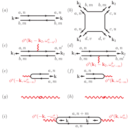
Figure S1: Feynman rules for both interacting RMT model and 2D disordered system: (a) shows a diagrammatic representation of the bare $X$ propagator; (b) illustrates the Hikami box that couples four $X$ matrices; (c)-(f) depict the interaction vertices coupling between the matrix field $X$ and the bosonic field $\phi$. (g) and (h) represent, respectively, the bare and interaction dressed $\phi$ propagators. (i) shows the leading order self-energy diagram for the bosonic field $\phi$. Note that the momentum labels are used for the 2D disordered system only.

In Figs. S1(a) and (g), we show the diagrammatic representations of the bare $X$ propagator $(\mathcal{G}^{(0)}_{X})^{ab;ba}_{nm;mn}$ and the bare $\phi$ propagator $\mathcal{G}_{\phi}^{(0)}$. We use two black solid lines with arrows pointing in the opposite directions to indicate the matrix fields $X$ and $X^{\dagger}$. The short arrows in between these two lines are introduced to distinguish $X$ (incoming arrow) and $X^{\dagger}$ (outgoing arrow). The red wavy line represents diagrammatically the bosonic field $\phi$, and the one with a open dot in the middle indicates the bare $\phi$ propagator $\mathcal{G}_{\phi}^{(0)}$ (see Fig. S1(g)). Fig. S1(b) depicts the four-point vertex which comes from the quartic action $S_{X}^{(4)}$, while Figs. S1(c)-(f) show the interaction vertices arising from the $\phi$-dependent part of the action $S_{X}^{(2)}$. The corresponding amplitudes are, in respective order,

$$\begin{aligned} &(b)=-i\frac{1}{2}\frac{J}{N}X^{\dagger}\,{}^{ab}_{nm}X^{bc}_{mu}X^{\dagger}\,{}^{cd}_{uv}X^{da}_{vn}\left(\zeta_{a}\varepsilon_{n}^{a}e^{-i\varepsilon_{n}^{a}\delta z_{a}}-\zeta_{b}\varepsilon_{m}^{b}e^{-i\varepsilon_{m}^{b}\delta z_{b}}+\zeta_{c}\varepsilon_{u}^{c}e^{-i\varepsilon_{u}^{c}\delta t_{c}}-\zeta_{d}\varepsilon_{v}^{d}e^{-i\varepsilon_{v}^{d}\delta t_{d}}\right),\\ &(c)=i\frac{1}{N}\sum\limits_{i}\phi^{a}_{ii}(\varepsilon_{n}^{a}-\varepsilon_{n^{\prime}}^{a})X^{\dagger}\,{}^{ba}_{mn}X^{ab}_{n^{\prime}m},\qquad(d)=-i\frac{1}{N}\sum\limits_{i}\phi^{b}_{ii}(\varepsilon_{m^{\prime}}^{b}-\varepsilon_{m}^{b})X^{\dagger}\,{}^{ba}_{mn}X^{ab}_{nm^{\prime}},\\ &(e)=\,-i\sqrt{\frac{2N}{J}}\frac{1}{N}\sum\limits_{i}\phi^{a}_{ii}(\varepsilon_{m}^{a}-\varepsilon_{n}^{a})X^{aa}_{nm},\quad\,\,\,(f)=-i\sqrt{\frac{2N}{J}}\frac{1}{N}\sum\limits_{i}\phi^{a}_{ii}(\varepsilon_{n}^{a}-\varepsilon_{m}^{a})X^{\dagger}\,{}^{aa}_{mn}.\end{aligned}$$ (S46)

I.4.2 Interaction dressed $\phi$ propagator

Taking into account the interactions between $\phi$ and $X$, we find that, to the leading order in small parameter $J/N$, the self-energy of the bosonic field $\phi$ is given by the diagram depicted in Fig. S1(i) with the analytical expression:

$$\begin{aligned} -i(\Sigma_{\phi})^{ab}_{ij;kl}(\omega_{m}^{a})=&-i\frac{1}{\pi}\frac{1}{JN}\zeta_{a}z_{a}(1-\delta_{m,0})\delta_{ab}\delta_{il}\delta_{jk}.\end{aligned}$$ (S47)

The full propagator for $\phi$ can be obtained from the Dyson equation, and takes the form

$$\begin{aligned} &i(\mathcal{G}_{\phi})^{ab}_{ij;kl}(\omega_{m}^{a})=\left[\left(-i(\mathcal{G}^{(0)}_{\phi})^{-1}+i\Sigma_{\phi}\right)^{-1}\right]^{ab}_{ij;kl}(\omega_{m}^{a})=i\zeta_{a}\frac{1}{z_{a}}\tilde{V}^{a}_{ij;kl}(\omega_{m}^{a})\delta_{ab},\end{aligned}$$ (S48)

where we have defined $\tilde{V}^{a}$ as

$$\begin{aligned} &(\tilde{V}^{a})^{-1}_{ij;kl}(\omega_{m}^{a})=V^{-1}_{ij;kl}+i\zeta_{a}\frac{1}{z_{a}}M^{a}_{m}\delta_{ik}\delta_{lj}-\frac{1}{\pi}\frac{1}{JN}(1-\delta_{m,0})\delta_{il}\delta_{jk}.\end{aligned}$$ (S49)

We use a red wavy line with a solid dot in the middle to denote the full $\phi$ propagator $\mathcal{G}_{\phi}$ (to distinguish it from the bare propagator $\mathcal{G}^{(0)}_{\phi}$ indicated by a open dot), see Fig. S1 (h).

I.4.3 Interaction dressed $X$ propagator

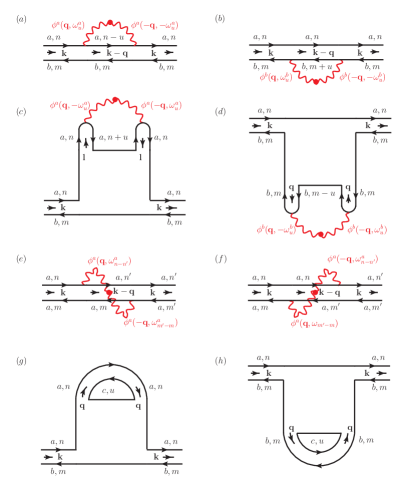
Figure S2: Leading order $X$ self energy diagrams for both the interacting RMT model and 2D disordered system. The momentum labels in all self-energy diagrams are used for the latter case.

In Fig. S2, we show the leading order self-energy diagrams for the matrix field $X$. In respective order, diagrams (a)-(f) give rise to the following contributions to the $X$ self-energy $\Sigma_{X}$:

$$\begin{aligned} (\Sigma^{(a)}_{X})^{ab;ba}_{nm;mn}=&-\frac{i}{N^{2}}\sum_{ij}\sum\limits_{u\leq n}\dfrac{1}{\zeta_{a}(\varepsilon_{n}^{a}-\omega_{u}^{a})e^{-i(\varepsilon_{n}^{a}-\omega_{u}^{a})\delta z_{a}}-\zeta_{b}\varepsilon_{m}^{b}e^{-i\varepsilon_{m}^{b}\delta z_{b}}}i\frac{\zeta_{a}}{z_{a}}\tilde{V}^{a}_{ij;ji}(\omega_{u}^{a}),\\ (\Sigma^{(b)}_{X})^{ab;ba}_{nm;mn}=&-\frac{i}{N^{2}}\sum_{ij}\sum\limits_{u<-m}\dfrac{1}{\zeta_{a}\varepsilon_{n}^{a}e^{-i\varepsilon_{n}^{a}\delta z_{a}}-\zeta_{b}(\varepsilon_{m}^{b}+\omega_{u}^{b})e^{-i(\varepsilon_{m}^{b}+\omega_{u}^{b})\delta z_{b}}}i\frac{\zeta_{b}}{z_{b}}\tilde{V}^{b}_{ij;ji}(\omega_{u}^{b}),\\ (\Sigma^{(c)}_{X})^{ab;ba}_{nm;mn}=&+i\frac{1}{N^{2}}\sum\limits_{ij}\sum\limits_{u<-n}\dfrac{\left[\zeta_{a}\varepsilon_{n}^{a}e^{-i\varepsilon_{n}^{a}\delta z_{a}}-\zeta_{b}\varepsilon_{m}^{b}e^{-i\varepsilon_{m}^{b}\delta z_{b}}+\zeta_{a}\varepsilon_{n}^{a}e^{-i\varepsilon_{n}^{a}\delta z_{a}}-\zeta_{a}(\varepsilon_{n}^{a}+\omega_{u}^{a})e^{-i(\varepsilon_{n}^{a}+\omega_{u}^{a})\delta z_{a}}\right]}{\left[\zeta_{a}\varepsilon_{n}^{a}e^{-i\varepsilon_{n}^{a}\delta z_{a}}-\zeta_{a}(\varepsilon_{n}^{a}+\omega_{u}^{a})e^{-i(\varepsilon_{n}^{a}+\omega_{u}^{a})\delta z_{a}}\right]^{2}}i\frac{\zeta_{a}}{z_{a}}\tilde{V}^{a}_{ij;ji}(\omega_{u}^{a}),\\ (\Sigma^{(d)}_{X})^{ab;ba}_{nm;mn}=&+i\frac{1}{N^{2}}\sum\limits_{ij}\sum\limits_{u\leq m}\dfrac{\left[\zeta_{a}\varepsilon_{n}^{a}e^{-i\varepsilon_{n}^{a}\delta z_{a}}-\zeta_{b}\varepsilon_{m}^{b}e^{-i\varepsilon_{m}^{b}\delta z_{b}}+\zeta_{b}(\varepsilon_{m}^{b}-\omega_{u}^{b})e^{-i(\varepsilon_{m}^{b}-\omega_{u}^{b})\delta z_{b}}-\zeta_{b}\varepsilon_{m}^{b}e^{-i\varepsilon_{m}^{b}\delta z_{b}}\right]}{\left[\zeta_{b}(\varepsilon_{m}^{b}-\omega_{u}^{b})e^{-i(\varepsilon_{m}^{b}-\omega_{u}^{b})\delta z_{b}}-\zeta_{b}\varepsilon_{m}^{b}e^{-i\varepsilon_{m}^{b}\delta z_{b}}\right]^{2}}i\frac{\zeta_{b}}{z_{b}}\tilde{V}^{b}_{ij;ji}(\omega_{u}^{b}),\\ (\Sigma^{(e)}_{X})\,^{aa;aa}_{nm;m^{\prime}n^{\prime}}=&+\frac{i}{N^{2}}\sum_{ij}\dfrac{1}{\zeta_{a}\varepsilon_{n^{\prime}}^{a}e^{-i\varepsilon_{n^{\prime}}^{a}\delta z_{a}}-\zeta_{a}\varepsilon_{m}^{a}e^{-i\varepsilon_{m}^{a}\delta z_{a}}}i\frac{\zeta_{a}}{z_{a}}\tilde{V}^{a}_{ij;ji}(\varepsilon_{n^{\prime}}^{a}-\varepsilon_{n}^{a})\delta_{n-n^{\prime},m-m^{\prime}},\\ (\Sigma^{(f)}_{X})\,^{aa;aa}_{nm;m^{\prime}n^{\prime}}=&+\frac{i}{N^{2}}\sum_{ij}\dfrac{1}{\zeta_{a}\varepsilon_{n}^{a}e^{-i\varepsilon_{n}^{a}\delta z_{a}}-\zeta_{a}\varepsilon_{m^{\prime}}^{a}e^{-i\varepsilon_{m^{\prime}}^{a}\delta z_{a}}}i\frac{\zeta_{a}}{z_{a}}\tilde{V}^{a}_{ij;ji}(\varepsilon_{n^{\prime}}^{a}-\varepsilon_{n}^{a})\delta_{n-n^{\prime},m-m^{\prime}},\end{aligned}$$ (S50)

where $n,n^{\prime}\geq 0>m,m^{\prime}$. We note that diagrams (g) and (h) contain a free replica summation $(\sum\limits_{c})$. Diagrams of this kind usually cancel with the Jacobian for parametrization Eq. S38 in NL$\sigma$M calculation, and as a result are ignored here.

The total contribution from all diagrams in Fig. S2(a)-(f) is composed of two parts:

$$(\Sigma_{X})\,^{ab;b^{\prime}a^{\prime}}_{nm;m^{\prime}n^{\prime}}=\left[(\Sigma_{\mathsf{diag}})\,^{ab;ba}_{nm;mn}\delta_{nn^{\prime}}\delta_{mm^{\prime}}+(\Sigma_{\mathsf{off}})\,^{aa;aa}_{nm;m^{\prime}n^{\prime}}\delta_{n-m,n^{\prime}-m^{\prime}}\delta_{ab}\right]\delta_{aa^{\prime}}\delta_{bb^{\prime}},\qquad n,n^{\prime}\geq 0>m,m^{\prime}.$$ (S51)

Here $\Sigma_{\mathsf{diag}}$ represents the contribution from diagrams (a)-(d), while $\Sigma_{\mathsf{off}}$ denotes the remaining contribution from diagrams (e)-(f) in Fig. S2. $\Sigma_{\mathsf{diag}}$ is diagonal in the Matsubara frequency space, meaning that the matrix element $(\Sigma_{\mathsf{diag}})\,^{ab;ba}_{nm;m^{\prime}n^{\prime}}$ is nonvanishing only when $n=n^{\prime}$ and $m=m^{\prime}$. By contrast, $\Sigma_{\mathsf{off}}$ has non-zero off-diagonal components in the frequency space. In addition, $\Sigma_{\mathsf{off}}^{ab;ba}$ vanishes when $a\neq b$, while $\Sigma_{\mathsf{diag}}^{ab;ba}$ takes non-zero value for any pair of $a$ and $b$.

The interaction dressed $X$ propagator $\mathcal{G}_{X}$ can be deduced from the Dyson equation for $X$

$$\begin{aligned} \sum\limits_{a^{\prime},b^{\prime}}\sum\limits_{n^{\prime}\geq 0>m^{\prime}}\left((\mathcal{G}^{(0)}_{X})^{-1}-\Sigma_{X}\right)^{ab;b^{\prime}a^{\prime}}_{nm;m^{\prime}n^{\prime}}(\mathcal{G}_{X})^{a^{\prime}b^{\prime};b^{\prime\prime}a^{\prime\prime}}_{n^{\prime}m^{\prime};m^{\prime\prime}n^{\prime\prime}}=\delta_{aa^{\prime\prime}}\delta_{bb^{\prime\prime}}\delta_{nn^{\prime\prime}}\delta_{mm^{\prime\prime}},\end{aligned}$$ (S52)

which reduces to the following equation for $a\neq b$ with the help of Eqs. S43 and S51,

$$\begin{aligned} (\mathcal{G}_{X})^{ab;b^{\prime\prime}a^{\prime\prime}}_{nm;m^{\prime\prime}n^{\prime\prime}}=\dfrac{1}{(\mathcal{G}^{(0)}_{X})^{-1}\,{}^{ab;ba}_{nm;mn}-\left(\Sigma_{\mathsf{dia}}\right)^{ab;ba}_{nm;mn}}\delta_{aa^{\prime\prime}}\delta_{bb^{\prime\prime}}\delta_{nn^{\prime\prime}}\delta_{mm^{\prime\prime}},\qquad\qquad\qquad\qquad\quad\,\,a\neq b.\end{aligned}$$ (S53)

In the following, we will call the $X$ propagator $\mathcal{G}_{X}^{ab;ba}$ ($X$ self-energy $\Sigma_{X}^{ab;ba}$) with $a\neq b$ the inter-replica propagator (inter-replica self-energy) and the one with $a=b$ the intra-replica propagator (intra-replica self-energy).

We emphasize that the intra-replica $X$ propagator $\mathcal{G}_{X}^{aa;aa}$ contribute to the disconnected part of the SFF

$$K^{\mathsf{dis}}(t)=\braket{Z(\eta+it)}\braket{Z(\eta-it)},$$ (S54)

while its inter-replica counterpart $\mathcal{G}_{X}^{a,-a;-a,a}$ is associated with the connected part of the SFF

$$K^{\mathsf{con}}(\eta,t)=\braket{Z(\eta+it)Z(\eta-it)}-\braket{Z(\eta+it)}\braket{Z(\eta-it)}.$$ (S55)

In this paper, we’re interested in the connected SFF $K_{\mathsf{con}}(t)$ which governs the ramp regime, and therefore will focus on the inter-replica propagator $\mathcal{G}_{X}^{a,-a;-a,a}$. The inter-replica $X$ propagator can be directly obtained from Eq. S53 after substituting the explicit forms of the bare propagator $(\mathcal{G}_{X}^{(0)})^{a,-a;-a,a}$ (Eq. S43) and the self-energy component $\Sigma_{\mathsf{dia}}^{a,-a;-a,a}$.

The self-energy component diagonal in the Matsubara frequency space $\Sigma_{\mathsf{diag}}$ is given by the summation of $\Sigma_{X}^{(a)}$ to $\Sigma_{X}^{(d)}$ in Eq. S50 and acquires the form of

$$(\Sigma_{\mathsf{diag}})\,^{ab;ba}_{nm;mn}=i\delta z(\zeta_{a}\varepsilon_{n}^{a}e^{-i\varepsilon_{n}^{a}\delta z_{a}}-\zeta_{b}\varepsilon_{m}^{b}e^{-i\varepsilon_{m}^{b}\delta z_{b}})-\lambda^{ab}_{nm}.$$ (S56)

Here $\delta z$ contributes to the renormalization effect and will be neglected in the following discussion. We believe the main interaction effect is from the mass term $\lambda^{ab}$ given by

$$\begin{aligned} \lambda^{ab}_{nm}=&\,\sum\limits_{-n\leq u\leq n}\dfrac{1}{z_{a}\omega_{u}^{a}}\sum_{ij}\frac{1}{N^{2}}\tilde{V}^{a}_{ij;ji}(\omega_{u}^{a})+\sum\limits_{m<u<-m}\dfrac{1}{z_{b}\omega_{u}^{b}}\sum_{ij}\frac{1}{N^{2}}\tilde{V}^{b}_{ij;ji}(\omega_{u}^{b}),\end{aligned}$$ (S57)

which is divergent at $u=0$. This infrared divergence can be curved by inclusion of higher order self-energy diagrams.

We use the self-consistent Born approximation (SCBA) to solve the infared divergence. In particular, we ignore all self-energy diagrams which contribute to the off-diagonal component in the Matsubara frequency space $\Sigma_{\mathsf{off}}$, and substitute the bare $X$ propagator $\mathcal{G}_{X}^{(0)}$ in the self-energy diagrams (a)-(d) with

$$\begin{aligned} (\mathcal{G}_{X}^{\prime})^{ab;ba}_{nm;mn}=\frac{1}{-i\left(\zeta_{a}\varepsilon_{n}^{a}e^{-i\varepsilon_{n}^{a}\delta z_{a}}-\zeta_{b}\varepsilon_{m}^{b}e^{-i\varepsilon_{m}^{b}\delta z_{b}}\right)+\lambda^{ab}_{nm}}.\end{aligned}$$ (S58)

We note that for $a\neq b$, this is the full interaction dressed inter-replica $X$ propagator (without considering the renormalization effect). For $a=b$, this propagator takes into account only the self-energy component $\Sigma_{\mathsf{dia}}^{aa;aa}$ but ignores $\Sigma_{\mathsf{off}}^{aa;aa}$. Using SCBA, we obtain the following self-consistent equation for the mass $\lambda^{ab}$:

$$\begin{aligned} \lambda^{ab}_{nm}=&+\sum\limits_{-n\leq u\leq n}\dfrac{1}{z_{a}\omega_{u}^{a}-i\zeta_{a}z_{a}\lambda^{ab}_{nm}}\sum_{ij}\frac{1}{N^{2}}\tilde{V}^{a}_{ij;ji}(\omega_{u}^{a})+\sum\limits_{m<u<-m}\dfrac{1}{z_{b}\omega_{u}^{b}-i\zeta_{b}z_{b}\lambda^{ab}_{nm}}\sum_{ij}\frac{1}{N^{2}}\tilde{V}^{b}_{ij;ji}(\omega_{u}^{b})\\ &+\sum\limits_{u<-n}\left(-\frac{z_{a}\omega_{u}^{a}}{\left(z_{a}\omega_{u}^{a}-i\zeta_{a}z_{a}\lambda^{aa}_{nn}\right)^{2}}+\frac{1}{z_{a}\omega_{u}^{a}-i\zeta_{a}z_{a}\lambda^{ab}_{nm}}\right)\sum\limits_{ij}\frac{1}{N^{2}}\tilde{V}^{a}_{ij;ji}(\omega_{u}^{a})\\ &+\sum\limits_{u\leq m}\left(-\frac{z_{b}\omega_{u}^{b}}{\left(z_{b}\omega_{u}^{b}-i\zeta_{b}z_{b}\lambda^{bb}_{mm}\right)^{2}}+\frac{1}{z_{b}\omega_{u}^{b}-i\zeta_{b}z_{b}\lambda^{ab}_{nm}}\right)\sum\limits_{ij}\frac{1}{N^{2}}\tilde{V}^{b}_{ij;ji}(\omega_{u}^{b}).\end{aligned}$$ (S59)

After summing over the Matsubara frequencies, this equation reduces to

$$\begin{aligned} &\lambda^{ab}_{nm}=\dfrac{\bar{V}_{0}^{a}}{2\pi}\dfrac{1}{-i\zeta_{a}z_{a}\lambda^{ab}_{nm}}+\dfrac{\bar{V}^{a}}{2\pi}\left[\begin{aligned} &-\psi(1-i\frac{\zeta_{a}z_{a}}{2\pi}\lambda^{ab}_{nm})+\psi(1-i\frac{\zeta_{a}z_{a}}{2\pi}\lambda^{ab}_{nm}+n)+\psi(1+i\frac{\zeta_{a}z_{a}}{2\pi}\lambda^{ab}_{nm})-\psi(1+i\frac{\zeta_{a}z_{a}}{2\pi}\lambda^{ab}_{nm}+n)\\ &+\psi(1+i\frac{\zeta_{a}z_{a}}{2\pi}\lambda^{ab}_{nm}+n)-\psi(1+i\frac{\zeta_{a}z_{a}}{2\pi}\lambda^{aa}_{nn}+n)-i\frac{\zeta_{a}z_{a}}{2\pi}\lambda^{aa}_{nn}\psi^{\prime}(1+i\frac{\zeta_{a}z_{a}}{2\pi}\lambda^{aa}_{nn}+n)\end{aligned}\right]\\ &+\dfrac{\bar{V}_{0}^{b}}{2\pi}\dfrac{1}{-i\zeta_{b}z_{b}\lambda^{ab}_{nm}}+\dfrac{\bar{V}^{b}}{2\pi}\left[\begin{aligned} &-\psi(1-i\frac{\zeta_{b}z_{b}}{2\pi}\lambda^{ab}_{nm})+\psi(1-i\frac{\zeta_{b}z_{b}}{2\pi}\lambda^{ab}_{nm}-m-1)+\psi(1+i\frac{\zeta_{b}z_{b}}{2\pi}\lambda^{ab}_{nm})-\psi(1+i\frac{\zeta_{b}z_{b}}{2\pi}\lambda^{ab}_{nm}-m-1)\\ &+\psi(1+i\frac{\zeta_{b}z_{b}}{2\pi}\lambda^{ab}_{nm}-m-1)-\psi(1+i\frac{\zeta_{b}z_{b}}{2\pi}\lambda^{bb}_{mm}-m-1)-i\frac{\zeta_{b}z_{b}}{2\pi}\lambda^{bb}_{mm}\psi^{\prime}(1+i\frac{\zeta_{b}z_{b}}{2\pi}\lambda^{bb}_{mm}-m-1)\end{aligned}\right],\end{aligned}$$ (S60)

where $\bar{V}^{a}$ and $\bar{V}^{a}_{0}$ are defined as $\sum_{ij}\frac{1}{N^{2}}\tilde{V}^{a}_{ij;ji}(\omega_{u}^{a})$ for $u\neq 0$ and $u=0$, respectively. The problem then reduces to solving three coupled self-consistent equations with three variables $\lambda^{+-}$, $\lambda^{++}$, $\lambda^{--}$. We have checked numerically that the solution to these self-consistent equations exist and it depends on the external frequency indices $n,m$ in addition to interaction matrix $V$ and complex time $z_{a}$.

Now let us consider what happen to the “zero modes” of the non-interacting theory after introducing the interactions. From Eq. S42 and earlier discussion about quadratic fluctuations, we can see that “zero modes” are encoded by $X^{ab}_{nm}$ and $X^{\dagger}\,{}^{ba}_{mn}$ for $a=-b$ and $m=-n-1$. It is straightforward to check that in the non-interacting theory ($\phi=0$), by setting $X^{ab}_{nm}=X^{\dagger}\,{}^{ab}_{nm}=0$ when $a\neq-b$ or $m\neq-n-1$, $S_{X}^{(2)}$ and $S_{X}^{(4)}$ (Eq. S40) as well as all higher order terms in the non-interacting action vanish. In the presence of interactions, we find from the caluclation above that that the soft modes encoded by $X^{a,-a}_{n,-n-1}$ and $X^{\dagger}\,{}^{-a,a}_{-n-1,n}$ acquire a mass $\lambda^{a,-a}$ (the solution to Eq. S60 with $b=-a$ and $m=-n-1$).

I.5 Contribution to the SFF from the soft modes around the standard saddle point

In terms of the interaction dressed propagators $\mathcal{G}_{X}$ and $\mathcal{G}_{\phi}$, we can express the contribution to the SFF from the standard saddle point $\Lambda^{(0)}$ and the corresponding fluctuations around it as

$$\begin{aligned} &K^{\prime}(\eta,t;\Lambda^{(0)})\propto e^{-S[\Lambda^{(0)},0]}\frac{\int\mathcal{D}\phi\exp\left[\frac{i}{2}\phi\mathcal{G}_{\phi}^{-1}\phi\right]\int\mathcal{D}(X^{\dagger},X)\exp\left(-\frac{N}{2J}X^{\dagger}\mathcal{G}_{X}^{-1}X\right)}{\int\mathcal{D}\phi\exp\left(-S_{\phi 0}[\phi]\right)\int\mathcal{D}(X^{\dagger},X)\exp\left(-\frac{N}{2J}X^{\dagger}X\right)}.\end{aligned}$$ (S61)

Here we have ignored the contribution from the massive modes, and kept only the leading order soft mode fluctuation correction. The two integrals in the denominators arise from the normalization constants $Z_{\phi}$ and $Z_{Q}$. As mentioned earlier, in the case of $\eta/(t^{2}+\eta^{2})\gtrsim{J}/{N}$, contributions from all remaining saddle points can be ignored, and the expression above gives approximately the SFF, i.e., $K(\eta,t)\approx K^{\prime}(\eta,t;\Lambda^{(0)})$. By contrast, for $\eta/(t^{2}+\eta^{2})\ll{J}/{N}$ (including $\eta=0$), all saddle points are equally important, and $K^{\prime}(\eta,t;\Lambda^{(0)})$ represents only the contribution associated with $\Lambda^{(0)}$.

For non-interacting case, we instead have

$$\begin{aligned} &K_{0}^{\prime}(\eta,t;\Lambda^{(0)})\propto e^{-S[\Lambda^{(0)},0]}\frac{\int\mathcal{D}(X^{\dagger},X)\exp\left(-\frac{N}{2J}X^{\dagger}(\mathcal{G}_{X}^{(0)})^{-1}X\right)}{\int\mathcal{D}(X^{\dagger},X)\exp\left(-\frac{N}{2J}X^{\dagger}X\right)},\end{aligned}$$ (S62)

which is consistent with Eq. S32. In the following, we will analyze the difference between $K^{\prime}(\eta,t;\Lambda^{(0)})$ (Eq. S61) and $K_{0}^{\prime}(\eta,t;\Lambda^{(0)})$ (Eq. S62), and in particular how the interaction effect influence the leading order fluctuation correction to the SFF.

Carrying out the integrations in Eq. S61 and Eq. S62 and using Eq. S48, we find

$$\begin{aligned} &K^{\prime}(\eta,t;\Lambda^{(0)})\propto e^{-S[\Lambda^{(0)},0]}\exp\left\{-\sum_{ab}\sum\limits_{n\geq 0>m}\ln\left((\mathcal{G}_{X}^{-1})^{ab;ba}_{nm;mn}\right)+\frac{1}{2}\sum\limits_{a,m}\left(\operatorname{Tr}\ln\tilde{V}^{a}(\omega_{m}^{a})-\operatorname{Tr}\ln V\right)\right\},\end{aligned}$$ (S63a)

$$\begin{aligned} &K^{\prime}_{0}(\eta,t;\Lambda^{(0)})\propto e^{-S[\Lambda^{(0)},0]}\exp\left\{-\sum_{ab}\sum\limits_{n\geq 0>m}\ln\left((\mathcal{G}_{X}^{(0)})^{-1}\,{}^{ab;ba}_{nm;mn}\right)\right\},\end{aligned}$$ (S63b)

where $\operatorname{Tr}$ indicates a trace over the flavor space only. In Eq.LABEL:eq:K2-2a (Eq.LABEL:eq:K2-2b), only the terms involving the inter-replica $X$ propagator $\mathcal{G}_{X}^{a,-a;-a,a}$ ($(\mathcal{G}_{X}^{(0)})^{a,-a;-a,a}$) contribute to the connected SFF $K^{\mathsf{con}}(\eta,t)$ ($K_{0}^{\mathsf{con}}(\eta,t)$). All remaining terms, including the ones associated with intra-replica $X$ propagator $\mathcal{G}_{X}^{aa;aa}$ ($(\mathcal{G}_{X}^{(0)})^{aa;aa}$) and $\phi$ propagator $\mathcal{G}_{\phi}$ contribute to the disconnected SFF $K^{\mathsf{dis}}(\eta,t)$ ($K_{0}^{\mathsf{dis}}(\eta,t)$). As mentioned earlier, we are interested in the connected SFF, and therefore will consider only the terms involving the inter-replica $X$ propagators in Eqs. LABEL:eq:K2-2a and LABEL:eq:K2-2b.

For $V\neq 0$, ignoring the renormalization effect and using Eq. S58, we find the contribution to $\ln K^{\prime\mathsf{con}}$ from the inter-replica $X$ propagator $\mathcal{G}_{X}^{ab;ba}$:

$$\begin{aligned} &\ln K^{\prime\mathsf{con}}(\eta,t;\Lambda^{(0)})=-\sum_{a\neq b}\sum\limits_{n\geq 0>m}\ln\left((\mathcal{G}_{X}^{-1})\,^{ab;ba}_{nm;mn}\right)=-\sum_{a\neq b}\sum\limits_{n\geq 0>m}\ln\left[-i\left(\zeta_{a}\varepsilon_{n}^{a}e^{-i\varepsilon_{n}^{a}\delta z_{a}}-\zeta_{b}\varepsilon_{m}^{b}e^{-i\varepsilon_{m}^{b}\delta z_{b}}\right)+\lambda^{ab}_{nm}\right].\end{aligned}$$ (S64)

We then use the anlytical continuation technique, and convert the double Matsubara summation in the equation above into a two-variables continous integral:

$$\begin{aligned} \ln K^{\prime\mathsf{con}}(\eta,t)=&\sum_{a\neq b}\int_{-\infty}^{\infty}\frac{d\varepsilon}{2\pi}\int_{-\infty}^{\infty}\frac{d\varepsilon^{\prime}}{2\pi}\ln\left(1+e^{-i\zeta_{a}z_{a}\varepsilon}\right)\ln\left(1+e^{-i\zeta_{b}z_{b}\varepsilon^{\prime}}\right)\\ &\times\left(\dfrac{1}{-i\left(\varepsilon-\varepsilon^{\prime}\right)+\lambda^{ab}(\zeta_{a}\varepsilon,\zeta_{b}\varepsilon^{\prime})}\right)^{2}\left(\frac{\partial\lambda^{ab}}{\partial\varepsilon}-i\right)\left(\frac{\partial\lambda^{ab}}{\partial\varepsilon^{\prime}}+i\right).\end{aligned}$$ (S65)

Here $\lambda^{ab}(\zeta_{a}\varepsilon,\zeta_{b}\varepsilon^{\prime})$ stands for $\lambda^{ab}_{nm}$ after the analytical continuation $\varepsilon_{n}^{a}\rightarrow\zeta_{a}\varepsilon$ and $\varepsilon_{m}^{b}\rightarrow\zeta_{b}\varepsilon^{\prime}$.

In the non-interacting case, the corresponding contribution can be found by replacing the interaction dressed propagator $\mathcal{G}_{X}^{ab;ba}$ with the bare one $(\mathcal{G}_{X}^{(0)})^{ab;ba}$, and setting the mass $\lambda^{ab}$ to $0$ in Eqs. S64 and S65, which leads to

$$\begin{aligned} \ln K_{0}^{\prime\mathsf{con}}(\eta,t)=&-\sum_{a\neq b}\sum\limits_{n>0>m}\operatorname{Tr}\ln(\mathcal{G}_{X}^{(0)}\,{}^{-1})^{ab;ba}_{nm;mn}\\ =&\sum_{a\neq b}\int_{-\infty}^{\infty}\frac{d\varepsilon}{2\pi}\int_{-\infty}^{\infty}\frac{d\varepsilon^{\prime}}{2\pi}\ln\left(1+e^{-i\zeta_{a}z_{a}\varepsilon}\right)\ln\left(1+e^{-i\zeta_{b}z_{b}\varepsilon^{\prime}}\right)\left(\dfrac{1}{-i\left(\varepsilon-\varepsilon^{\prime}\right)}\right)^{2}.\end{aligned}$$ (S66)

In Ref. Liao et al. (2020), using a cumulant expansion, we showed that, to study the quadratic order fluctuation correction to the non-interacting SFF $K_{0}(\eta,t)$, one can replace $\ln\left(1+e^{-i\zeta_{a}z_{a}\varepsilon}\right)\ln\left(1+e^{-i\zeta_{b}z_{a}\varepsilon^{\prime}}\right)$ with $e^{-i\zeta_{a}z_{a}\varepsilon-i\zeta_{b}z_{b}\varepsilon^{\prime}}$. The neglected term from this replacement cancels partially with higher order contributions. See also the discussion in Sec. I.6. We apply the same substitution here for both the interacting and non-interacting theories, with the focus placed on the difference between the two cases, and find that Eq. S65 and Eq. S66 become, respectively,

$$\begin{aligned} \ln K^{\prime\prime\mathsf{con}}(\eta,t)=&\sum\limits_{a}\int_{-\infty}^{\infty}\frac{d\varepsilon}{2\pi}\int_{-\infty}^{\infty}\frac{d\varepsilon^{\prime}}{2\pi}e^{-i\zeta_{a}t(\varepsilon-\varepsilon^{\prime})}e^{-\eta(\varepsilon+\varepsilon^{\prime})}\left(\dfrac{1}{-i\left(\varepsilon-\varepsilon^{\prime}\right)+\lambda^{a,-a}(\zeta_{a}\varepsilon,-\zeta_{a}\varepsilon^{\prime})}\right)^{2}\\ &\times\left(\frac{\partial\lambda^{a,-a}}{\partial\varepsilon}-i\right)\left(\frac{\partial\lambda^{a,-a}}{\partial\varepsilon^{\prime}}+i\right)\\ =&\sum\limits_{a}\int_{-E_{\mathsf{UV}}}^{E_{\mathsf{UV}}}\frac{dE}{2\pi}\int_{-\infty}^{\infty}\frac{d\omega}{2\pi}e^{-2\eta E}e^{-i\zeta_{a}t\omega}\left(\dfrac{1}{-i\omega+\lambda^{a,-a}(E)}\right)^{2}\left[\left(\frac{1}{2}\frac{\partial\lambda^{a,-a}(E)}{\partial E}\right)^{2}+1\right]\\ =&\sum\limits_{a}\int_{-E_{\mathsf{UV}}}^{E_{\mathsf{UV}}}\frac{dE}{2\pi}e^{-2\eta E}te^{-\zeta_{a}\lambda^{a,-a}(E)t}\Theta(\zeta_{a}\operatorname{Re}\lambda^{a,-a}(E))\left[\left(\frac{1}{2}\frac{\partial\lambda^{a,-a}(E)}{\partial E}\right)^{2}+1\right],\end{aligned}$$ (S67)

and

$$\begin{aligned} \ln K_{0}^{\mathsf{con}}\,{}^{\prime\prime}(\eta,t)=&\sum\limits_{a}\int_{-\infty}^{\infty}\frac{d\varepsilon}{2\pi}\int_{-\infty}^{\infty}\frac{d\varepsilon^{\prime}}{2\pi}e^{-i\zeta_{a}t(\varepsilon-\varepsilon^{\prime})}e^{-\eta(\varepsilon+\varepsilon^{\prime})}\left(\dfrac{1}{-i\left(\varepsilon-\varepsilon^{\prime}\right)}\right)^{2}\\ =&-\sum\limits_{a}\int_{-E_{\mathsf{UV}}}^{E_{\mathsf{UV}}}\frac{dE}{2\pi}e^{-2\eta E}\int_{-\infty}^{\infty}\frac{d\omega}{2\pi}e^{-i\zeta_{a}t\omega}\dfrac{1}{\omega^{2}}.\end{aligned}$$ (S68)

Here in the second equalities of both equations, we have made the transformation

$$\begin{aligned} \omega=\varepsilon-\varepsilon^{\prime},\qquad E=\frac{1}{2}(\varepsilon+\varepsilon^{\prime}).\end{aligned}$$ (S69)

We have also employed the box approximation which ignores the energy dependence of average bare single-particle density of states and imposes the ultraviolet cutoff $E_{\mathsf{UV}}$ (see Refs. Liao et al. (2020); Cotler et al. (2017); Liu (2018)). Furthermore, in Eq. S67 we have assumed that $\lambda^{a,-a}$ depends on $E$ but not $\omega$ (the $\omega$-dependent part contributes to the renormalization and can be neglected).

For $\eta/(t^{2}+\eta^{2})\gtrsim{J}/{N}$, Eqs. S67 and S68 represent approximately the leading order fluctuation correction to $\ln K^{\mathsf{con}}(\eta,t)$ in the interacting and non-interacting cases, respectively. Taking the $\eta\rightarrow 0^{+}$ limit and comparing these two equations, we can see that the presence of inter-replica mass $\lambda^{\pm,\mp}$ results in the suppression of exponential growth of the connected SFF, which is necessary for the emergence of RMT statistics in many-body energy spectrum. We emphasize that Eqs. S67 and S68 only takes into account the contribution from leading order fluctuations. Superficially, it might seems that corrections from higher order fluctuations are of higher order in $J/N$, but they are in fact non-negligible and essential to extract the explicit expression for the SFF.

I.6 Cumulant expansion and higher order fluctuations

To see that the contribution from higher order fluctuations is crucial to the derivation of the explicit form of the SFF, let us first consider the non-interacting case. Setting the decoupling field $\phi$ to $0$ and integrating out the fermionic field $\psi$ in Eq. S8, we find that the non-interacting SFF can be written as

$$\begin{aligned} K_{0}(\eta,t)=&\left\langle\exp\left\{\sum\limits_{a,n}\operatorname{Tr}\ln\left[-iz_{a}\left(\varepsilon_{n}^{a}e^{-i\varepsilon_{n}^{a}\delta z_{a}}I_{f}-\zeta_{a}h\right)\right]\right\}\right\rangle,\end{aligned}$$ (S70)

Converting the summation over Matsubara frequency $\varepsilon_{n}^{a}=\frac{2\pi}{z_{a}}(n+\frac{1}{2})$ into a continuous integral, the above equation becomes

$$\begin{aligned} K_{0}(\eta,t)=\left\langle\exp\left\{N\sum\limits_{a}\int_{-\infty}^{\infty}d\varepsilon\ln\left[1+e^{-i\zeta_{a}z_{a}\varepsilon}\right]\nu(\varepsilon)\right\}\right\rangle,\end{aligned}$$ (S71)

where $\nu(\varepsilon)$ is the single-particle density of states:

$$\nu(\varepsilon)=\frac{1}{N}\operatorname{Tr}\delta(\varepsilon-h).$$ (S72)

After a cumulant expansion of Eq. (S71) Liao et al. (2020), we obtain

$$\begin{aligned} \ln K_{0}(\eta,t)=\,&N\int_{-\infty}^{\infty}d\varepsilon\sum\limits_{a}\ln\left(1+e^{-i\zeta_{a}z_{a}\varepsilon}\right)\mathtt{R}_{1}(\varepsilon)\\ &+\frac{N^{2}}{2}\int_{-\infty}^{\infty}d\varepsilon\int_{-\infty}^{\infty}d\varepsilon^{\prime}\left[\sum\limits_{a}\ln\left(1+e^{-i\zeta_{a}z_{a}\varepsilon}\right)\right]\left[\sum\limits_{b}\ln\left(1+e^{-i\zeta_{b}z_{b}\varepsilon^{\prime}}\right)\right]\mathtt{R}_{2}^{\mathsf{con}}(\varepsilon,\varepsilon^{\prime})\\ &+...+\frac{N^{n}}{n!}\int_{-\infty}^{\infty}...\int_{-\infty}^{\infty}\left\{\prod_{k=1}^{n}d\varepsilon_{k}\left[\sum\limits_{a_{k}}\ln\left(1+e^{-i\zeta_{a_{k}}z_{a_{k}}\varepsilon_{k}}\right)\right]\right\}\mathtt{R}_{n}^{\mathsf{con}}(\varepsilon_{1},...,\varepsilon_{n})+...\,\,\,.\end{aligned}$$ (S73)

Here $\mathtt{R}_{n}^{\mathsf{con}}(\varepsilon_{1},...,\varepsilon_{n})$ is the connected part of the bare $n$-point single-particle energy level correlation function $\mathtt{R}_{n}(\varepsilon_{1},...,\varepsilon_{n})$, which is defined as

$$\begin{aligned} \mathtt{R}_{n}(\varepsilon_{1},...,\varepsilon_{n})=\left\langle\nu(\varepsilon_{1})...\nu(\varepsilon_{n})\right\rangle.\end{aligned}$$ (S74)

It is known that, for a GUE ensemble following the probability $P(h)$ in Eq. S2, the two-level connected correlation function assumes the form Mehta (2004); Guhr et al. (1998)

$$\begin{aligned} N^{2}\mathtt{R}_{2}^{\mathsf{con}}(\varepsilon,\varepsilon^{\prime})=-\frac{1-\cos\left(2N(\varepsilon-\varepsilon^{\prime})/J\right)}{2\pi^{2}(\varepsilon-\varepsilon^{\prime})^{2}}+\frac{N}{\pi J}\delta(\varepsilon-\varepsilon^{\prime}),\end{aligned}$$ (S75)

which at $|\varepsilon-\varepsilon^{\prime}|\gg J/N$ can be approximated as

$$\begin{aligned} N^{2}\mathtt{R}_{2}^{\mathsf{con}}(\varepsilon,\varepsilon^{\prime})=-\frac{1}{2\pi^{2}(\varepsilon-\varepsilon^{\prime})^{2}}.\end{aligned}$$ (S76)

Substituting this expression into Eq. S73, we find that the second term on the right-hand side of Eq. S73 is equivalent to Eq. S66 after restoring the contribution to the disconnected SFF from the intra-replica $X$ propagators (restoring $a=b$ terms). In other words, the quadratic order fluctuation correction obtained earlier yields the second order term in the cumulant expansion:

$$\begin{aligned} &-\sum_{a,b}\sum\limits_{n>0>m}\operatorname{Tr}\ln(\mathcal{G}_{X}^{(0)}\,{}^{-1})^{ab;ba}_{nm;mn}=\frac{N^{2}}{2}\sum\limits_{a,b}\int_{-\infty}^{\infty}d\varepsilon\int_{-\infty}^{\infty}d\varepsilon^{\prime}\ln\left(1+e^{-i\zeta_{a}z_{a}\varepsilon}\right)\ln\left(1+e^{-i\zeta_{b}z_{b}\varepsilon^{\prime}}\right)\mathtt{R}_{2}^{\mathsf{con}}(\varepsilon,\varepsilon^{\prime})\end{aligned}$$ (S77)

To recover the contribution from the oscillatory part of $\mathtt{R}_{2}^{\mathsf{con}}(\varepsilon,\varepsilon^{\prime})$ (the $\cos$ term in Eq. S75), one needs to consider fluctuations around the nonstandard saddle points Andreev and Altshuler (1995).

Using Eqs. S16 and S18, we find that the action at the standard saddle point $\Lambda^{(0)}$ is equivalent to the first term in the cumulant expansion in Eq. S73:

$$\begin{aligned} S[\Lambda^{(0)},0]=-N\int_{-\infty}^{\infty}d\varepsilon\sum\limits_{a}\ln\left(1+e^{-i\zeta_{a}z_{a}\varepsilon}\right)\mathtt{R}_{1}(\varepsilon),\end{aligned}$$ (S78)

where the average single-particle level density is given by

$$\mathtt{R}_{1}(\varepsilon)=\frac{1}{2\pi J^{2}}\sqrt{4J^{2}-\varepsilon^{2}}.$$ (S79)

Combining Eqs. S77 and S78, one can see that Eq. LABEL:eq:K2-2a obtained from considering only the quadratic order soft mode fluctuations yields only the leading two terms in the cumulant expansions. It has been found in Ref. Liao et al. (2020) that all higher order terms in the cumulant expansion are equally important in the ramp region, and they are essential to extract the correct overall coefficient in the exponent of ramp expression. For this reason, we believe the higher order correction is indispensable for the derivation the SFF.

Note that the level correlation function is sometimes defined differently in some literatures Mehta (2004), and $\mathtt{R}_{n}$ here contains several $\delta$ functions for $n\geq 2$ (see for example Eq. S75). In Ref. Liao et al. (2020), we show that if one throws away all $\delta$-functions in $\mathtt{R}_{n}^{\mathsf{con}}$ and at the same time replaces $\sum\limits_{a}\ln(1+e^{-i\zeta_{a}z_{a}\varepsilon})$ with $\frac{1}{2}\prod_{a}\left(1+e^{-i\zeta_{a}z_{a}\varepsilon}\right)-1$, the left hand side of Eq. S73 remains the same up to some unessential constant. This justifies the replacement $\ln\left(1+e^{-i\zeta_{a}z_{a}\varepsilon}\right)\ln\left(1+e^{-i\zeta_{b}z_{a}\varepsilon^{\prime}}\right)\rightarrow e^{-i\zeta_{a}z_{a}\varepsilon-i\zeta_{b}z_{b}\varepsilon^{\prime}}$ performed in Eqs. S67 and S68.

In the presence of interactions, as shown in the earlier section, the contribution from the quadratic order fluctuations to $K^{\mathsf{con}}(\eta,t)$ is also given by the second term in the cumulant expansion Eq. S73 (with $a\neq b$) after making the replacement

$$\begin{aligned} 2\pi^{2}N^{2}\mathtt{R}_{2}^{\mathsf{con}}(\varepsilon,\varepsilon^{\prime})=-\frac{1}{(\varepsilon-\varepsilon^{\prime})^{2}}\rightarrow\left(\frac{1}{-i(\varepsilon-\varepsilon^{\prime})+\lambda}\right)^{2}\left(\frac{\partial\lambda^{ab}}{\partial\varepsilon}-i\right)\left(\frac{\partial\lambda^{ab}}{\partial\varepsilon^{\prime}}+i\right),\qquad|\varepsilon-\varepsilon^{\prime}|\gg J/N\end{aligned}$$ (S80)

We expect that, for higher order fluctuations, the interaction effect will be similar and the corresponding contribution to the SFF is also be suppressed because of the inter-replica masses $\lambda^{\pm,\mp}$. However, this is beyond the scope of the current study.

II Disordered interacting systems in 2D

In this section, we will perform an analogous calculation of the SFF for a two-dimensional disordered interacting system of spinless fermions with broken time reversal symmetry, which falls into the unitary Wigner-Dyson class and is governed by the following Hamiltonian

$$\begin{aligned} H=\int d^{2}\bm{\mathrm{r}}\,\psi^{\dagger}(\bm{\mathrm{r}})\left(-\frac{\nabla^{2}}{2m}-\mu+U_{\mathsf{imp}}(\bm{\mathrm{r}})\right)\psi(\bm{\mathrm{r}})+\frac{1}{2}\int d^{2}\bm{\mathrm{r}}\int d^{2}\bm{\mathrm{r}}^{\prime}\psi^{\dagger}(\bm{\mathrm{r}})\psi^{\dagger}(\bm{\mathrm{r}}^{\prime})V(|\bm{\mathrm{r}}-\bm{\mathrm{r}}^{\prime}|)\psi(\bm{\mathrm{r}}^{\prime})\psi(\bm{\mathrm{r}}).\end{aligned}$$ (S81)

Here $U_{\mathsf{imp}}(\bm{\mathrm{r}})$ represents the random impurity potential, and follows the Gaussian distribution function

$$P(U_{\mathsf{imp}})=\frac{1}{Z_{U}}\exp{\left[-\pi\nu_{0}\tau_{\mathsf{el}}\int\limits_{\bm{\mathrm{r}}}U_{\mathsf{imp}}^{2}(\bm{\mathrm{r}})\right]},\qquad Z_{U}=\int\mathcal{D}U_{\mathsf{imp}}\exp\left[-\pi\nu_{0}\tau_{\mathsf{el}}\int\limits_{\bm{\mathrm{r}}}U_{\mathsf{imp}}^{2}(\bm{\mathrm{r}})\right],$$ (S82)

where $\nu_{0}$ denotes the bare average single-particle density of states at Fermi energy $\mu$, and $\tau_{\mathsf{el}}$ indicates the elastic scattering time. For simplicity, we consider short-range density-density interactions with $V(r)=V\delta(r)$. The current calculation can be generalized to other types of interaction. As in the previous section, we calculate the SFF $K(\eta,t)=\braket{Z(\eta+it)Z(\eta-it)}$, where the angular bracket now indicates averaging over the ensemble of random impurity potential $U_{\mathsf{imp}}(\bm{\mathrm{r}})$ according to the distribution function $P(U_{\mathsf{imp}})$ in Eq. S82. We will focus on the time regime $\Delta^{-1}\gg t\gg\tau_{\mathsf{el}}$, where $\Delta\equiv 1/\nu_{0}L^{2}$ is the average bare single-particle level spacing, with $L\rightarrow\infty$ being system size. We also consider weak enough disorder so that a perturbation in terms of disorder strength can be performed.

II.1 Preliminaries

The SFF for this disordered interacting fermion system can be expressed as the following path integral:

$$\begin{aligned} K(\eta,t)=&\frac{1}{Z_{U}}\int\mathcal{D}U_{\mathsf{imp}}\exp\left(-\pi\nu_{0}\tau_{\mathsf{el}}\int\limits_{\bm{\mathrm{r}}}U_{\mathsf{imp}}^{2}(\bm{\mathrm{r}})\right)\\ \times&\int\mathcal{D}(\bar{\psi},\psi)\exp\left\{i\sum\limits_{a=\pm}\int_{0}^{z_{a}}dt^{\prime}\int\limits_{\bm{\mathrm{r}}}\bar{\psi}^{a}(\bm{\mathrm{r}},t^{\prime})\left[i\partial_{t^{\prime}}-\zeta_{a}\left(-\frac{\nabla^{2}}{2m}-\mu+U_{\mathsf{imp}}(\bm{\mathrm{r}})\right)\right]\psi^{a}(\bm{\mathrm{r}},t^{\prime})\right\}\\ \times&\exp\left\{-\frac{i}{2}\sum\limits_{a=\pm}\zeta_{a}\int_{0}^{z_{a}}dt^{\prime}\int\limits_{\bm{\mathrm{r}}}\bar{\psi}^{a}(\bm{\mathrm{r}},t^{\prime})\bar{\psi}^{a}(\bm{\mathrm{r}},t^{\prime})V\psi^{a}(\bm{\mathrm{r}},t^{\prime})\psi^{a}(\bm{\mathrm{r}},t^{\prime})\right\}.\end{aligned}$$ (S83)

The Grassmann fields $\bar{\psi}^{a}$ and $\psi^{a}$ carry a replica index $a=\pm$ which corresponds to the forward/backward path for $Z(\eta\pm it)$, and they are subject to the antiperiodic boundary condition Eq. S6. Complex time $z_{a}$ is defined as $z_{a}=t-i\zeta_{a}\eta$ with $\zeta_{a}=\pm 1$ for $a=\pm$.

Introducing an auxiliary bosonic field $\phi$ to decouple the interactions, we obtain

$$\begin{aligned} &K(\eta,t)=\,\frac{1}{Z_{U}Z_{\phi}}\int\mathcal{D}U_{\mathsf{imp}}\exp\left[-\pi\nu_{0}\tau_{\mathsf{el}}\int\limits_{\bm{\mathrm{r}}}U_{\mathsf{imp}}^{2}(\bm{\mathrm{r}})\right]\int\mathcal{D}\phi\exp\left(\sum\limits_{a,n}\frac{i}{2}\zeta_{a}z_{a}\int\limits_{\bm{\mathrm{r}}}\phi^{a}_{-n}(\bm{\mathrm{r}})V^{-1}\phi^{a}_{n}(\bm{\mathrm{r}})\right)\\ \times&\int\mathcal{D}(\bar{\psi},\psi)\exp\left\{\begin{aligned} \sum\limits_{a,n,m}iz_{a}\int\limits_{\bm{\mathrm{r}}}\bar{\psi}^{a}_{n}(\bm{\mathrm{r}})\left\{\varepsilon_{n}^{a}e^{-i\varepsilon_{n}^{a}\delta z_{a}}\delta_{nm}-\zeta_{a}\left(-\frac{\nabla^{2}}{2m}-\mu+U_{\mathsf{imp}}(\bm{\mathrm{r}})\right)\delta_{nm}+\zeta_{a}\phi^{a}_{n-m}(\bm{\mathrm{r}})\right\}\psi^{a}_{m}(\bm{\mathrm{r}})\end{aligned}\right\}.\end{aligned}$$ (S84)

Here we have performed a temporal Fourier transformation of the fermionic field $\psi$ as in Eq. S7, and similarly for the bosonic field $\phi$. The normalization constant $Z_{\phi}$ is given by $Z_{\phi}=\int\mathcal{D}\phi\exp\left(\sum\limits_{a,n}\frac{i}{2}\zeta_{a}z_{a}\int_{\bm{\mathrm{r}}}\phi_{-n}^{a}(\bm{\mathrm{r}})V^{-1}\phi_{n}^{a}(\bm{\mathrm{r}})\right)$.

To proceed, we perform the ensemble averaging in Eq. S84, and decouple the generated quartic term by a Hermitian matrix field $Q(\bm{\mathrm{r}})$:

$$\begin{aligned} &K_{\eta}(\eta,t)=\,\frac{1}{Z_{\phi}Z_{Q}}\int\mathcal{D}\phi\exp\left(\frac{i}{2}\sum\limits_{a,n}\zeta_{a}z_{a}\int\limits_{\bm{\mathrm{r}}}\phi_{-n}^{a}(\bm{\mathrm{r}})V^{-1}\phi_{n}^{a}(\bm{\mathrm{r}})\right)\int\mathcal{D}Q\exp\left(-\frac{\pi\nu_{0}}{4\tau_{\mathsf{el}}}\int\limits_{\bm{\mathrm{r}}}\operatorname{Tr}Q^{2}(\bm{\mathrm{r}})\right)\\ \times&\int\mathcal{D}(\bar{\psi},\psi)\exp\left\{\begin{aligned} \sum\limits_{a,b,n,m}iz_{a}\int\limits_{\bm{\mathrm{r}}}\bar{\psi}_{n}^{a}(\bm{\mathrm{r}})\left[\left(\varepsilon_{n}^{a}e^{-i\varepsilon_{n}^{a}\delta z_{a}}\zeta_{a}+\frac{\nabla^{2}}{2m}+\mu\right)\delta_{nm}\delta_{ab}+\phi_{n-m}^{a}(\bm{\mathrm{r}})\delta_{ab}+\frac{i}{2\tau_{\mathsf{el}}}Q_{nm}^{ab}(\bm{\mathrm{r}})\right]\zeta_{b}\psi_{m}^{b}(\bm{\mathrm{r}})\end{aligned}\right\},\end{aligned}$$ (S85)

where the normalization constant is $Z_{Q}=\int\mathcal{D}Q\exp\left(-\frac{\pi\nu_{0}}{4\tau_{\mathsf{el}}}\int\limits_{\bm{\mathrm{r}}}\operatorname{Tr}Q^{2}(\bm{\mathrm{r}})\right)$. After integrating out the fermionic field $\psi$ and performing the spatial Fourier transformation,

$$\begin{aligned} \phi(\bm{\mathrm{q}})=\frac{1}{L^{2}}\int d^{2}\bm{\mathrm{r}}\phi(\bm{\mathrm{r}})e^{-i\bm{\mathrm{q}}\cdot\bm{\mathrm{r}}},\qquad Q(\bm{\mathrm{q}})=\frac{1}{L^{2}}\int d^{2}\bm{\mathrm{r}}Q(\bm{\mathrm{r}})e^{-i\bm{\mathrm{q}}\cdot\bm{\mathrm{r}}},\end{aligned}$$ (S86)

we arrive at the following $\sigma-$model

$$K(\eta,t)=\,\frac{1}{Z_{\phi}Z_{Q}}\int\mathcal{D}\phi\exp\left(-S_{\phi 0}[\phi]\right)\int\mathcal{D}Q\exp\left(-S_{\phi 0}[\phi]-S[Q,\phi]\right),$$ (S87a)

$$S_{\phi 0}[\phi]=-\frac{i}{2}\sum\limits_{a}\zeta_{a}z_{a}L^{2}\sum\limits_{\bm{\mathrm{q}},m}\phi_{-m}^{a}(-\bm{\mathrm{q}})V^{-1}\phi_{m}^{a}(\bm{\mathrm{q}}),$$ (S87b)

$$S[Q,\phi]=\,\frac{\pi\nu_{0}}{4\tau_{\mathsf{el}}}L^{2}\sum\limits_{\bm{\mathrm{q}}}\operatorname{Tr}Q(\bm{\mathrm{q}})Q(-\bm{\mathrm{q}})-\operatorname{Tr}\ln\left[\left(\mathcal{E}\sigma^{3}-\xi_{\bm{\mathrm{k}}}\right)\delta_{\bm{\mathrm{q}},0}+\frac{i}{2\tau_{\mathsf{el}}}Q(\bm{\mathrm{q}})+\Phi(\bm{\mathrm{q}})\right]+\text{const}.,$$ (S87c)

with $\xi_{\bm{\mathrm{k}}}=k^{2}/2m-\mu$. The second $\operatorname{Tr}$ in Eq. S87c represents a trace over momentum space in addition to the Matsubara frequency and replica spaces. $\mathcal{E}$, $\Phi(\bm{\mathrm{q}})$, and $\sigma^{3}$ are defined such that their matrices elements are given by $\mathcal{E}^{ab}_{nm}=\delta_{nm}\delta_{ab}\varepsilon_{n}^{a}e^{-i\varepsilon_{n}^{a}\delta z_{a}}$ , $\Phi^{ab}_{nm}(\bm{\mathrm{q}})=\delta_{ab}\phi^{a}_{n-m}(\bm{\mathrm{q}})$, and $(\sigma^{3})^{ab}_{nm}=\zeta_{a}\delta_{ab}\delta_{nm}$, respectively.

II.2 The saddle points

Starting from the action $S[Q,\phi]$ in Eq. S87c and ignoring the influence of the decoupling field $\phi$, we now look for saddle point $Q_{sp}$ of the matrix field. Taking variation of the non-interacting action $S[Q,0]$ over $Q$, we find that the saddle point $Q_{sp}$ is determined by the equation

$$\begin{aligned} Q_{sp}(\bm{\mathrm{q}})=\frac{i}{\pi}\frac{1}{\nu_{0}L^{2}}\sum_{\bm{\mathrm{k}}}\left[\left(\mathcal{E}\sigma^{3}-\xi_{\bm{\mathrm{k}}}\right)\delta_{\bm{\mathrm{q}},0}+\frac{i}{2\tau_{\mathsf{el}}}Q_{sp}(-\bm{\mathrm{q}})\right]^{-1}.\end{aligned}$$ (S88)

We first look for spatially uniform solution $Q_{sp}(\bm{\mathrm{q}})=\Lambda\delta_{\bm{\mathrm{q}},0}$ diagonal in Matsubara frequency and replica spaces. Assuming weak enough disorder such that the chemical potential $\mu\gg\tau_{\mathsf{el}}^{-1}$, and neglecting the variation of single-particle density states near the Fermi surface, we find

$$\Lambda_{nm}^{ab}=s_{n}^{a}\delta_{nm}\delta_{ab},\qquad s_{n}^{a}=\pm 1.$$ (S89)

We therefore obtain a series of spatially uniform saddle points diagonal in both Matsubara frequency and replica spaces, corresponding to different choices of $\left\{s_{n}^{a}\right\}$.

The non-interacting action $S[Q,\phi=0]$ (see Eq. S87c) is invariant under any spatially uniform unitary rotation $Q\rightarrow R^{-1}\Lambda R$ without the symmetry breaking term $\mathcal{E}\sigma^{3}$. In the limits $|\delta z_{a}|,\eta\rightarrow 0$, one can find that the symmetry transformation $U$, under which the non-interacting action $S[Q,\phi=0]$ remains invariant, is given by direct product of multiple spatially uniform $U(2)$ rotations $U=\prod_{n}U_{n}$. Here $U_{n}$ rotates only the matrix subblock $\begin{bmatrix}Q^{++}_{nn}&Q^{+-}_{n,-n-1}\\ Q^{-+}_{-n-1,n}&Q^{--}_{-n-1,-n-1}\end{bmatrix}$ as in Eq. S19. New saddle points can be generated by applying the symmetry transformation $U$ to the diagonal saddle points $Q\rightarrow U^{-1}\Lambda U$.

At a diagonal saddle point $\Lambda$, the non-interacting action $S[Q,\phi=0]$ acquires the form

$$\begin{aligned} S[\Lambda,0]=\sum\limits_{n}\sum\limits_{a}i\frac{\pi}{\Delta}\zeta_{a}\varepsilon_{n}^{a}s_{n}^{a}e^{-i\varepsilon_{n}^{a}\delta z_{a}}+\text{const}.\end{aligned}$$ (S90)

As in the previous section, we assume that $|\delta z_{a}|/t^{2}\ll\Delta$ and the phase factor $e^{-i\varepsilon_{n}^{a}\delta z_{a}}$ is only needed when there is a convergence issue. In the case of $\eta/(t^{2}+\eta^{2})\gtrsim\Delta$, we can see from Eq. S90 that the symmetry breaking $\eta$ determines the standard saddle point which minimizes the real part of the non-interacting action $\operatorname{Re}S[\Lambda,0]$ among various saddle points. The standard saddle point is given by

$$(\Lambda^{(0)})^{aa}_{nn}=\operatorname{sgn}(n+1/2),$$ (S91)

and yields the dominant contribution. By contrast, when $\eta/(t^{2}+\eta^{2})\ll\Delta$ (including $\eta=0$), it is important to keep contributions from all saddle points which only differ by phases.

II.3 Quadratic fluctuations and the non-interacting SFF

We now consider the fluctuations $\delta Q$ of the matrix field $Q$ around a diagonal saddle point $\Lambda$, as well as the H.S. decoupling field $\phi$. Up to quadratic order in $\delta Q=Q-\Lambda$ and $\phi$, $S[Q,\phi]$ can be expressed as

$$\begin{aligned} &\delta S[\delta Q,\phi;\Lambda^{(s)}]\equiv S[\Lambda^{(s)}+\delta Q,\phi]-S[\Lambda^{(s)},0]=\sum\limits_{\bm{\mathrm{q}}}\sum\limits_{a,b,m,n}M_{nm}^{ab}(\bm{\mathrm{q}})\delta Q_{nm}^{ab}(\bm{\mathrm{q}})\delta Q_{mn}^{ba}(-\bm{\mathrm{q}})+\sum\limits_{a}M^{\prime a}\phi^{a}_{0}(\bm{\mathrm{0}})\\ &+\sum\limits_{\bm{\mathrm{q}}}\sum\limits_{a,m,n}\bar{M}^{a}_{nm}(\bm{\mathrm{q}})\delta Q_{nm}^{aa}(\bm{\mathrm{q}})\phi^{a}_{m-n}(-\bm{\mathrm{q}})+\frac{1}{2}\sum\limits_{\bm{\mathrm{q}}}\sum\limits_{a,m}\tilde{M}^{a}_{m}\phi^{a}_{-m}(-\bm{\mathrm{q}})\phi^{a}_{m}(\bm{\mathrm{q}}).\end{aligned}$$ (S92)

$M$, $M^{\prime}$, $\bar{M}$ and $\bar{M}$ depend on the saddle point $\Lambda$ and acquire the forms

$$\begin{aligned} M^{ab}_{nm}(\bm{\mathrm{q}})=\,&\frac{\pi}{4\tau_{\mathsf{el}}\Delta}\left(1-\frac{\Delta}{2\tau_{\mathsf{el}}\pi}\sum\limits_{\bm{\mathrm{k}}}G^{a}_{n}(\bm{\mathrm{k}})G^{b}_{m}(\bm{\mathrm{k}}-\bm{\mathrm{q}})\right)\\ \approx&\frac{\pi}{4\tau_{\mathsf{el}}\Delta}\left\{1-\left(1-\delta_{s_{m}^{b},s_{n}^{a}}\right)\left[1-i\tau_{\mathsf{el}}s_{n}^{a}\left(\zeta_{b}\varepsilon_{m}^{b}e^{-i\varepsilon_{m}^{b}\delta z_{b}}-\zeta_{a}\varepsilon_{n}^{a}e^{-i\varepsilon_{n}^{a}\delta z_{a}}\right)-\tau_{\mathsf{el}}Dq^{2}\right]\right\},\\ M^{\prime a}=\,&-\sum\limits_{\bm{\mathrm{k}}}\sum\limits_{n}G^{a}_{n}(\bm{\mathrm{k}})=i\frac{\pi}{\Delta}\sum\limits_{n}s_{n}^{a},\\ \bar{M}^{a}_{nm}(\bm{\mathrm{q}})=\,&i\frac{1}{2\tau_{\mathsf{el}}}\sum\limits_{\bm{\mathrm{k}}}G^{a}_{n}(\bm{\mathrm{k}})G^{a}_{m}(\bm{\mathrm{k}}-\bm{\mathrm{q}})\approx i\frac{\pi}{\Delta}\left(1-\delta_{s_{m}^{a},s_{n}^{a}}\right),\\ \tilde{M}^{a}_{m}=\,&\sum\limits_{\bm{\mathrm{k}}}\sum_{n}G^{a}_{n}(\bm{\mathrm{k}})G^{a}_{n+m}(\bm{\mathrm{k}}+\bm{\mathrm{q}})\approx\sum\limits_{\bm{\mathrm{k}}}\sum_{n}\left[G^{a}(\bm{\mathrm{k}},\varepsilon_{n})\right]^{2},\end{aligned}$$ (S93)

where $D=v_{\mathsf{F}}^{2}\tau_{\mathsf{el}}/2$ is the diffuson constant and $G$ is defined as

$$G^{a}_{n}(\bm{\mathrm{k}})=\dfrac{1}{\zeta_{a}\varepsilon_{n}^{a}e^{-i\varepsilon_{n}^{a}\delta z_{a}}-\xi_{\bm{\mathrm{k}}}+\frac{i}{2\tau_{\mathsf{el}}}s_{n}^{a}}.$$ (S94)

From Eq. S92, one can immediately see that the bare propagator of $\delta Q$ is determined by the matrix kernel $M$. Depending on the values of $M^{ab}_{nm}(\bm{\mathrm{q}})$, the fluctuations $\delta Q^{ab}_{nm}(\bm{\mathrm{q}})$ and $\delta Q^{ba}_{mn}(-\bm{\mathrm{q}})$ fall into two different categories: the massive mode and the soft mode.

1. When $s_{n}^{a}=s_{m}^{b}$, $M^{ab}_{nm}(\bm{\mathrm{q}})$ is given approximately by a constant

   $$M^{ab}_{nm}(\bm{\mathrm{q}})=\frac{\pi}{4\tau_{\mathsf{el}}\Delta},$$ (S95)

   and the associated $\delta Q^{ab}_{nm}(\bm{\mathrm{q}})$ and $\delta Q^{ba}_{mn}(-\bm{\mathrm{q}})$ are massive mode fluctuations.

2. By contrast, when $s_{n}^{a}=-s_{m}^{b}$, we have

   $$M^{ab}_{nm}(\bm{\mathrm{q}})=\frac{\pi}{4\Delta}\left[is_{n}^{a}\left(\zeta_{b}\varepsilon_{m}^{b}e^{-i\varepsilon_{m}^{b}\delta z_{b}}-\zeta_{a}\varepsilon_{n}^{a}e^{-i\varepsilon_{n}^{a}\delta z_{a}}\right)+Dq^{2}\right],$$ (S96)

   and the corresponding fluctuations belong to a special type of soft mode named diffuson. These soft modes can be generated by spatial dependent unitary rotation of the saddle point:

   $$Q(\bm{\mathrm{r}})=R^{-1}(\bm{\mathrm{r}})\Lambda R(\bm{\mathrm{r}}).$$ (S97)

   In the special case when $a=-b$, $n=-m-1$ and $\bm{\mathrm{q}}=0$, Eq. S96 becomes

   $$M^{a,-a}_{n,-n-1}(0)=\frac{\pi}{\Delta}s_{n}^{a}\frac{\eta}{t^{2}+\eta^{2}}\pi(n+1/2).$$ (S98)

   $M^{a,-a}_{n,-n-1}(0)$ vanishes when $\eta/(t^{2}+\eta^{2})\ll 1/\Delta$, but assumes the value of $M^{a,-a}_{n,-n-1}(0)\gtrsim 1$ when $\eta/(t^{2}+\eta^{2})\gtrsim 1/\Delta$. The corresponding soft modes are the zero modes generated by symmetry transformation, i.e., $R(\bm{\mathrm{r}})$ applied to the $\Lambda$ in Eq. S97 becomes the spatial uniform symmetry transformation $U$.

Combing Eqs. S87a and S92, we find that the contribution to the SFF from a diagonal saddle point $\Lambda^{(s)}$ and small fluctuations around it $\delta Q^{(s)}=Q-\Lambda^{(s)}$ can be expressed as

$$\begin{aligned} &K^{\prime}(\eta,t;\Lambda^{(s)})=\,\frac{-S[\Lambda^{(s)},0]}{Z_{\phi}Z_{Q}}\int\mathcal{D}\phi e^{-S_{\phi 0}[\phi]}\int\mathcal{D}\delta Q^{(s)}\exp\left(-\delta S[\delta Q^{(s)},\phi;\Lambda^{(s)}]\right).\end{aligned}$$ (S99)

In the non-interacting case, after setting $\phi=0$ in the equation above, we obtain

$$\begin{aligned} &K_{0}^{\prime}(\eta,t;\Lambda^{(s)})=\,e^{-S[\Lambda^{(s)},0]}\dfrac{\int\mathcal{D}\delta Q^{(s)}\exp\left(-\sum\limits_{\bm{\mathrm{q}}}\sum\limits_{a,b,m,n}M_{nm}^{ab}(\bm{\mathrm{q}})(\delta Q^{(s)})_{nm}^{ab}(\bm{\mathrm{q}})(\delta Q^{(s)})_{mn}^{ba}(-\bm{\mathrm{q}})\right)}{\int\mathcal{D}\delta Q^{(s)}\exp\left(-\frac{\pi}{4\tau_{\mathsf{el}}\Delta}\sum\limits_{\bm{\mathrm{q}}}\sum\limits_{a,b,m,n}(\delta Q^{(s)})_{nm}^{ab}(\delta Q^{(s)})_{mn}^{ba}\right)}.\end{aligned}$$ (S100)

The integration over each pair of $\delta Q^{ab}_{mn}(\bm{\mathrm{q}})$ and $\delta Q^{ba}_{nm}(-\bm{\mathrm{q}})$ gives rise to a factor of $4\tau_{\mathsf{el}}\Delta/\pi M^{ab}_{nm}(\bm{\mathrm{q}})$ after taking into account the corresponding contribution from the normalization constant $Z_{Q}$, as long as $M^{ab}_{nm}(\bm{\mathrm{q}})\neq 0$. This leads to

$$\begin{aligned} &K_{0}(\eta,t)=\,\sum\limits_{s}e^{-S[\Lambda^{(s)},0]}\exp\left[-\sum\limits_{\bm{\mathrm{q}},a,b,m,n}^{\prime}\ln\left(\frac{4\tau_{\mathsf{el}}\Delta}{\pi}M_{nm}^{ab}(\bm{\mathrm{q}})\right)\right]\mathcal{Z}_{0}^{(s)},\end{aligned}$$ (S101)

where the summation $\sum_{\bm{\mathrm{q}},a,b,m,n}^{\prime}$ excludes the zero modes. The contribution from zero modes denoted by $\mathcal{Z}_{0}^{(s)}$ here might seem to be divergent in the limit of $\eta\rightarrow 0^{+}$ at the quadratic order. However, as mentioned earlier, taking into account higher order fluctuations, one finds

$$\begin{aligned} &\mathcal{Z}_{0}^{(s)}=\,\mathcal{V}_{0}^{(s)}\exp\left[-\frac{1}{2}\mathcal{N}_{0}^{(s)}\ln\left(4\tau_{\mathsf{el}}\Delta\right)\right].\end{aligned}$$ (S102)

$\mathcal{N}_{0}^{(s)}$ stands for the number of the zero modes, and $\mathcal{V}_{0}^{(s)}$ denotes the volume of the associated saddle point manifold generated by $Q_{sp}=U^{-1}\Lambda^{(s)}U$, where $U$ belongs to the symmetry group of the non-interacting theory Kamenev and Mézard (1999b).

We can see from Eq. S101 that the massive modes give rise to a nonessential constant. By contrast, the soft mode fluctuations off-diagonal in the replica space ($\delta Q^{ab}$ with $a\neq b$) lead to the exponential ramp (see more details in the following sections). From the analysis of saddle point action, we believe that the SFF for $\eta/(t^{2}+\eta^{2})\gtrsim\Delta$ can be approximated by the contribution associated with the standard saddle point $K(\eta,t)\approx K^{\prime}(\eta,t;\Lambda^{(0)})$. In the opposite limit $\eta/(t^{2}+\eta^{2})\gtrsim\Delta$, it is also necessary to take into account the contributions from fluctuations around nonstandard points.

II.4 Nonlinear $\sigma$-model for the standard saddle point

Let us now focus on the soft mode fluctuations around the standard saddle point $\Lambda^{(0)}$ and investigate their interactions with the H.S. decoupling field $\phi$. These soft modes are generated by rotation of $\Lambda^{(0)}$, and can be expressed as

$$Q(\bm{\mathrm{r}})=R^{-1}(\bm{\mathrm{r}})\Lambda^{(0)}R(\bm{\mathrm{r}}),$$ (S103)

where $R(\bm{\mathrm{r}})\in U(2N_{\varepsilon})/U(N_{\varepsilon})\times U(N_{\varepsilon})$, with $N_{\varepsilon}$ being the total number of Matsubara frequencies smaller than the ultraviolet cutoff $|\varepsilon_{n}^{\pm}|\leq\tau_{\mathsf{el}}^{-1}$. For zero modes, $Q$ can also be expressed as Eq. S103 with $R(\bm{\mathrm{r}})=U\in\prod_{n=1}^{N_{\varepsilon}}U(2)/U(1)\times U(1)$ being a special spatial uniform unitary rotation which leaves the non-interacting action $S[Q,0]$ invariant when $\eta=0$.

We employ the parameterization Eq. S103 and insert it into the action $S[Q,\phi]$ (Eq. S87c). After expanding the $\operatorname{Tr}\ln$ term in gradients of the rotation matrix $R$ and the decoupling field $\phi$, we arrive at the nonlinear $\sigma-$model describing soft mode fluctuations of $Q$ matrix around the standard saddle point $\Lambda^{(0)}$ :

$$\begin{aligned} \delta S[Q,\phi;\Lambda^{(0)}]\equiv&S[Q,\phi]-S[\Lambda^{(0)},0]\\ =&\frac{\pi}{4\Delta}D\sum\limits_{\bm{\mathrm{q}}}q^{2}\operatorname{Tr}\left[Q(\bm{\mathrm{q}})Q(-\bm{\mathrm{q}})\right]+i\frac{\pi}{\Delta}\operatorname{Tr}\left[\mathcal{E}\sigma^{3}\left(Q(\bm{\mathrm{0}})-\Lambda^{(0)}\right)\right]\\ &+i\frac{\pi}{\Delta}\sum\limits_{\bm{\mathrm{q}}}\sum\limits_{a,n,m}Q^{aa}_{nm}(\bm{\mathrm{q}})\phi^{a}_{m-n}(-\bm{\mathrm{q}})+\frac{1}{2}\sum\limits_{\bm{\mathrm{q}}}\sum\limits_{a,m}\tilde{M}^{a}_{m}\phi^{a}_{m}(-\bm{\mathrm{q}})\phi^{a}_{m}(\bm{\mathrm{q}}).\end{aligned}$$ (S104)

Here $\tilde{M}^{a}_{m}$ is defined in Eq. S93 and takes the value of $\tilde{M}^{a}_{m}=-i\zeta_{a}z_{a}/\Delta$ for the standard saddle point $\Lambda^{(0)}$ (Eq. S91). $Q$ is subject to the following constraints,

$$\begin{aligned} \operatorname{Tr}Q(\bm{\mathrm{r}})=0,\qquad Q^{2}(\bm{\mathrm{r}})=I,\qquad Q^{\dagger}(\bm{\mathrm{r}})=Q(\bm{\mathrm{r}}).\end{aligned}$$ (S105)

It can be reparameterized as

$$\begin{aligned} &\begin{array}[]{cc}\quad m\geq 0&\qquad\qquad\qquad m<0\end{array}\\ Q_{nm}(\bm{\mathrm{r}})=&\begin{bmatrix}\sqrt{I-X(\bm{\mathrm{r}})X^{\dagger}(\bm{\mathrm{r}})}&X(\bm{\mathrm{r}})\\ X^{\dagger}(\bm{\mathrm{r}})&-\sqrt{I-X^{\dagger}(\bm{\mathrm{r}})X(\bm{\mathrm{r}})}\end{bmatrix}\begin{array}[]{c}n\geq 0\\ n<0\\ \end{array},\end{aligned}$$ (S106)

which resolves the constraints automatically. $X^{ab}_{nm}(\bm{\mathrm{r}})$ ($X^{\dagger}\,{}^{ab}_{nm}(\bm{\mathrm{r}})$) is an unconstrained $N_{\varepsilon}\times N_{\varepsilon}$ complex matrix labeled with nonnegative (negative) frequency row index $n$ and negative (nonnegative) frequency column index $m$ in addition to replica indices $a,b$.

We then substitute Eq. S106 into Eq. S104 and expand in terms of matrix fields $X$ and $X^{\dagger}$. One can see, after a rescaling similar to Eq. S39 (see also Ref. Liao et al. (2017)), that terms of higher order in $X$ and $X^{\dagger}$ are also of higher order in disorder strength. We keep the terms up to quadratic order in $X$ in the total action $\delta S[Q,\phi;\Lambda^{(0)}]$ as well as the quartic terms in the $\phi$-independent part of the action,

$$\delta S^{\prime}[Q,\phi;\Lambda^{(0)}]=\,S_{\phi}+S_{X}^{(2)}+S_{X}^{(4)},$$ (S107a)

$$S_{\phi}=\,\frac{1}{2}\sum\limits_{\bm{\mathrm{q}}}\sum\limits_{a,m}\tilde{M}^{a}_{m}\phi^{a}_{-m}(-\bm{\mathrm{q}})\phi^{a}_{m}(\bm{\mathrm{q}}),$$ (S107b)

$$\begin{aligned} S_{X}^{(2)}=\,&\sum\limits_{\bm{\mathrm{k}}_{1},\bm{\mathrm{k}}_{2}}\sum\limits_{abcd}\sum\limits_{m,m^{\prime}\geq 0>n,n^{\prime}}X^{\dagger}\,{}^{ab}_{nm}(\bm{\mathrm{k}}_{1})D^{ba;dc}_{mn;n^{\prime}m^{\prime}}(\bm{\mathrm{k}}_{1},\bm{\mathrm{k}}_{2})X^{cd}_{m^{\prime}n^{\prime}}(\bm{\mathrm{k}}_{2})\\ &+\sum\limits_{\bm{\mathrm{k}}}\sum\limits_{ab}\sum\limits_{m>0>n}\left[\bar{J}\,^{ab}_{nm}(\bm{\mathrm{k}})X\,^{ba}_{mn}(\bm{\mathrm{k}})+X^{\dagger}\,{}^{ab}_{nm}(\bm{\mathrm{k}})J\,^{ba}_{mn}(\bm{\mathrm{k}})\right],\end{aligned}$$ (S107c)

$$\begin{aligned} &S_{X}^{(4)}=\frac{\pi}{16\Delta}\sum\limits_{\bm{\mathrm{k}}_{1},\bm{\mathrm{k}}_{2},\bm{\mathrm{k}}_{3},\bm{\mathrm{k}}_{4}}\sum\limits_{abcd}\sum\limits_{m,v\geq 0>n,u}\delta_{\bm{\mathrm{k}}_{1}+\bm{\mathrm{k}}_{3},\bm{\mathrm{k}}_{2}+\bm{\mathrm{k}}_{4}}X^{\dagger}\,{}^{ab}_{nm}(\bm{\mathrm{k}}_{1})X^{bc}_{mu}(\bm{\mathrm{k}}_{2})X^{\dagger}\,{}^{cd}_{uv}(\bm{\mathrm{k}}_{3})X^{da}_{vn}(\bm{\mathrm{k}}_{4})\\ &\times\left[-2D(\bm{\mathrm{k}}_{1}\cdot\bm{\mathrm{k}}_{3}+\bm{\mathrm{k}}_{2}\cdot\bm{\mathrm{k}}_{4})+D(\bm{\mathrm{k}}_{1}+\bm{\mathrm{k}}_{3})\cdot(\bm{\mathrm{k}}_{2}+\bm{\mathrm{k}}_{4})+i\left(\zeta_{a}\varepsilon_{n}^{a}e^{-i\varepsilon_{n}^{a}\delta z_{a}}-\zeta_{b}\varepsilon_{m}^{b}e^{-i\varepsilon_{m}^{b}\delta z_{b}}+\zeta_{c}\varepsilon_{u}^{c}e^{-i\varepsilon_{u}^{c}\delta t_{c}}-\zeta_{d}\varepsilon_{v}^{d}e^{-i\varepsilon_{v}^{d}\delta t_{d}}\right)\right].\end{aligned}$$ (S107d)

Here $\mathcal{K}$, $\bar{J}$ and $J$ are defined as

$$\begin{aligned} &\mathcal{K}^{ba;dc}_{mn;n^{\prime}m^{\prime}}(\bm{\mathrm{k}}_{1},\bm{\mathrm{k}}_{2})=\delta_{ad}\delta_{bc}\frac{\pi}{2\Delta}\left\{\left[Dk_{1}^{2}+i\left(\zeta_{a}\varepsilon_{n}^{a}e^{-i\varepsilon_{n}^{a}\delta z_{a}}-\zeta_{b}\varepsilon_{m}^{b}e^{-i\varepsilon_{m}^{b}\delta z_{b}}\right)\right]\delta_{mm^{\prime}}\delta_{nn^{\prime}}\delta_{\bm{\mathrm{k}}_{1},\bm{\mathrm{k}}_{2}}\right.\\ &\left.\qquad\qquad\qquad\qquad-i\delta_{nn^{\prime}}\phi^{b}_{m-m^{\prime}}(\bm{\mathrm{k}}_{1}-\bm{\mathrm{k}}_{2})+i\delta_{mm^{\prime}}\phi^{a}_{n^{\prime}-n}(\bm{\mathrm{k}}_{1}-\bm{\mathrm{k}}_{2})\right\},\\ &\bar{J}^{ab}_{nm}(\bm{\mathrm{k}})=\delta_{ab}i\frac{\pi}{\Delta}\phi^{a}_{n-m}(-\bm{\mathrm{k}}),\qquad J\,^{ba}_{mn}(\bm{\mathrm{k}})=\delta_{ab}i\frac{\pi}{\Delta}\phi^{a}_{m-n}(\bm{\mathrm{k}}).\end{aligned}$$ (S108)

If one equates $\delta Q_{nm}^{ab}(\bm{\mathrm{q}})$ with $X^{ab}_{nm}(\bm{\mathrm{q}})$ for $n\geq 0>m$ and $X^{\dagger}\,{}^{ab}_{nm}(-\bm{\mathrm{q}})$ for $m\geq 0>n$, the action derived earlier by considering only the quadratic order fluctuations, i.e., Eq. S92, is consistent with the first few terms in Eq. S107 as expected.

II.4.1 Feynman rules

From the quadratic action $S_{X}^{(2)}$ (Eq. S107c), we find the bare $X$ propagator, i.e., the bare diffuson propagator

$$\begin{aligned} (\mathcal{G}^{(0)}_{X}\,)^{ab;b^{\prime}a^{\prime}}_{nm;m^{\prime}n^{\prime}}(\bm{\mathrm{k}},\bm{\mathrm{k}}^{\prime})\equiv\braket{X^{ab}_{nm}(\bm{\mathrm{k}})X^{\dagger}\,{}^{b^{\prime}a^{\prime}}_{m^{\prime}n^{\prime}}(\bm{\mathrm{k}}^{\prime})}_{0}=\frac{2\Delta}{\pi}\mathcal{D}_{0}(\bm{\mathrm{k}},\zeta_{a}\varepsilon_{n}^{a}e^{-i\varepsilon_{n}^{a}\delta z_{a}}-\zeta_{b}\varepsilon_{m}^{b}e^{-i\varepsilon_{m}^{b}\delta z_{b}})\delta_{nn^{\prime}}\delta_{mm^{\prime}}\delta_{a,a^{\prime}}\delta_{b,b^{\prime}}\delta_{\bm{\mathrm{k}},\bm{\mathrm{k}}^{\prime}},\end{aligned}$$ (S109)

where we have defined

$$\begin{aligned} \mathcal{D}_{0}(\bm{\mathrm{k}};\omega)=\frac{1}{Dk^{2}-i\omega}.\end{aligned}$$ (S110)

The bare propagator of the H.S. decoupling field $\phi$ arises from the part of the action involving only the bosonic field $\phi$, including $S_{\phi 0}$ (Eq. S87b) and $S_{\phi}$ (Eq. S107b), and takes the form of

$$\begin{aligned} i\left[\mathcal{G}_{\phi}^{(0)}(\bm{\mathrm{q}},\omega_{m}^{a})\right]^{ab}=\braket{\phi^{a}_{m}(\bm{\mathrm{q}})\phi^{b}_{-m}(-\bm{\mathrm{q}})}_{0}=i\delta_{ab}\frac{\zeta_{a}}{z_{a}}\left[L^{2}V^{-1}+i\frac{\zeta_{a}}{z_{a}}\tilde{M}_{m}^{a}\right]^{-1}=i\delta_{ab}\frac{\zeta_{a}}{z_{a}}\gamma\Delta,\end{aligned}$$ (S111)

where

$$\begin{aligned} \gamma\equiv&\dfrac{\Delta^{-1}}{L^{2}V^{-1}+\Delta^{-1}}=\dfrac{\nu_{0}}{V^{-1}+\nu_{0}}.\end{aligned}$$ (S112)

The diagrammatic representations of the bare $X$ and $\phi$ propagators are depicted in Figs. S1 (a) and (g), respectively. As for the previous RMT model, the double solid black lines with oppositely directed arrows indicate the matrix field $X$, while the red wavy line denotes the bosonic $\phi$. In Figs. S1 (b)-(f), we also show the 4-point vertex for matrix field $X$ as well as the interaction vertices that couple $X$ and $\phi$. The corresponding analytical expressions are as follows:

$$\begin{aligned} &(b)=-\frac{\pi}{8\Delta}\delta_{\bm{\mathrm{k}}_{1}+\bm{\mathrm{k}}_{3},\bm{\mathrm{k}}_{2}+\bm{\mathrm{k}}_{4}}X^{\dagger}\,{}^{ab}_{nm}(\bm{\mathrm{k}}_{1})X^{bc}_{mu}(\bm{\mathrm{k}}_{2})X^{\dagger}\,{}^{cd}_{uv}(\bm{\mathrm{k}}_{3})X^{da}_{vn}(\bm{\mathrm{k}}_{4})\\ &\times\left[-2D(\bm{\mathrm{k}}_{1}\cdot\bm{\mathrm{k}}_{3}+\bm{\mathrm{k}}_{2}\cdot\bm{\mathrm{k}}_{4})+D(\bm{\mathrm{k}}_{1}+\bm{\mathrm{k}}_{3})\cdot(\bm{\mathrm{k}}_{2}+\bm{\mathrm{k}}_{4})+i\left(\zeta_{a}\varepsilon_{n}^{a}e^{-i\varepsilon_{n}^{a}\delta z_{a}}-\zeta_{b}\varepsilon_{m}^{b}e^{-i\varepsilon_{m}^{b}\delta z_{b}}+\zeta_{c}\varepsilon_{u}^{c}e^{-i\varepsilon_{u}^{c}\delta t_{c}}-\zeta_{d}\varepsilon_{v}^{d}e^{-i\varepsilon_{v}^{d}\delta t_{d}}\right)\right],\\ &(c)=+i\frac{\pi}{2\Delta}\phi^{a}_{n-n^{\prime}}(\bm{\mathrm{k}}_{1}-\bm{\mathrm{k}}_{2})X^{\dagger}\,{}^{ba}_{mn}(\bm{\mathrm{k}}_{1})X^{ab}_{n^{\prime}m}(\bm{\mathrm{k}}_{2}),\qquad(d)=-i\frac{\pi}{2\Delta}\phi^{b}_{m^{\prime}-m}(\bm{\mathrm{k}}_{1}-\bm{\mathrm{k}}_{2})X^{\dagger}\,{}^{ba}_{mn}(\bm{\mathrm{k}}_{1})X^{ab}_{nm^{\prime}}(\bm{\mathrm{k}}_{2}),\\ &(f)=-i\frac{\pi}{\Delta}\phi^{a}_{m-n}(-\bm{\mathrm{k}})X\,^{aa}_{nm}(\bm{\mathrm{k}}),\qquad\qquad\qquad\qquad\quad\,\,(e)=-i\frac{\pi}{\Delta}\phi^{a}_{n-m}(\bm{\mathrm{k}})X^{\dagger}\,{}^{aa}_{mn}(\bm{\mathrm{k}}).\end{aligned}$$ (S113)

II.4.2 Interaction dressed $\phi$ propagator

The leading order self-energy diagram for the bosonic field $\phi$ is shown in Fig. S1(i) and its analytical expression takes the form of

$$\begin{aligned} -i\Sigma_{\phi}^{ab}(\bm{\mathrm{q}},\omega_{m}^{a})=&-\delta_{ab}\frac{2\pi}{\Delta}\sum\limits_{0>n\geq-|m|}\frac{1}{Dq^{2}-i\zeta_{a}\left(\varepsilon_{n+|m|}^{a}e^{-i\varepsilon_{n+|m|}^{a}\delta z_{a}}-\varepsilon_{n}^{a}e^{-i\varepsilon_{n}^{a}\delta z_{a}}\right)}\\ =&-\delta_{ab}\frac{z_{a}}{\Delta}\frac{\omega_{|m|}^{a}}{Dq^{2}-i\zeta_{a}\omega_{|m|}^{a}}.\end{aligned}$$ (S114)

Here we have used

$$\begin{aligned} \sum\limits_{0>n\geq-|m|}=|m|=z_{a}\frac{\omega_{|m|}^{a}}{2\pi}.\end{aligned}$$ (S115)

Inserting this result into the Dyson equation for bosonic field $\phi$, we find the interaction dressed $\phi$ propagator

$$\begin{aligned} i\mathcal{G}_{\phi}^{ab}(\bm{\mathrm{q}},\omega_{m}^{a})=\left[\left(-i\mathcal{G}^{(0)}_{\phi}\,{}^{-1}(\bm{\mathrm{q}},\omega_{m}^{a})+i\Sigma_{\phi}(\bm{\mathrm{q}},\omega_{m}^{a})\right)^{-1}\right]^{ab}=i\delta_{ab}\zeta_{a}\frac{\gamma\Delta}{z_{a}}\dfrac{\mathcal{D}_{\gamma}(\bm{\mathrm{q}},\zeta_{a}\omega_{|m|}^{a})}{\mathcal{D}_{0}(\bm{\mathrm{q}},\zeta_{a}\omega_{|m|}^{a})},\end{aligned}$$ (S116)

where $D_{\gamma}(\bm{\mathrm{k}},\omega)$ is defined as

$$\begin{aligned} \mathcal{D}_{\gamma}(\bm{\mathrm{k}},\omega)=\frac{1}{Dk^{2}-i(1-\gamma)\omega}.\end{aligned}$$ (S117)

We use a red wavy line with a solid dot to represent diagrammatically the dressed $\phi$ propagator $\mathcal{G}_{\phi}$ (Fig. S1(h)), and for the bare $\phi$ propagator $\mathcal{G}_{\phi}^{(0)}$ the solid dot is replaced with an open one (Fig. S1(g)).

II.4.3 Interaction dressed diffuson propagator

For matrix field $X$, the leading order self-energy diagrams are shown in Fig. S2, and their total contribution can be expressed as a summation of two parts:

$$(\Sigma_{X})\,^{ab;b^{\prime}a^{\prime}}_{nm;m^{\prime}n^{\prime}}(\bm{\mathrm{k}},\bm{\mathrm{k}}^{\prime})=\left[(\Sigma_{\mathsf{diag}})\,^{ab;ba}_{nm;mn}(\bm{\mathrm{k}};\bm{\mathrm{k}})\delta_{n,n^{\prime}}\delta_{m,m^{\prime}}+(\Sigma_{\mathsf{off}})\,^{aa;aa}_{nm;m^{\prime}n^{\prime}}(\bm{\mathrm{k}};\bm{\mathrm{k}})\delta_{n-m,n^{\prime}-m^{\prime}}\delta_{ab}\right]\delta_{aa^{\prime}}\delta_{bb^{\prime}}\delta_{\bm{\mathrm{k}},\bm{\mathrm{k}}^{\prime}}.$$ (S118)

$\Sigma_{\mathsf{diag}}$ is diagonal in the Matsubara frequency space and represents the contribution from diagrams (a)-(d) in Fig. S2. The remaining contribution from diagrams (e)-(f) in Fig. S2 is denoted as $\Sigma_{\mathsf{off}}$ with nonvanishing off-diagonal components in the Matsubara frequency space (i.e. $(\Sigma_{\mathsf{off}})_{nm;m^{\prime}n^{\prime}}$ is non-zero for $m^{\prime}\neq m$ and $n^{\prime}\neq n$). We emphasize that $\Sigma_{\mathsf{off}}^{ab;ba}$ vanishes when $a\neq b$ and therefore is irrelevant to the inter-replica $X$ propagator $\mathcal{G}_{X}^{a,-a;-a,a}$. Self-energy diagrams (g) and (h) in Fig. S2 are not considered here as this kind of diagrams usually cancel with the Jacobian from the parameterization Eq. S106.

The analytical expressions for diagrams (a)-(f) in Fig. S2 are given by, in respective order,

$$\begin{aligned} (\Sigma^{(a)}_{X})^{ab;ba}_{nm;mn}(\bm{\mathrm{k}},\bm{\mathrm{k}})=&-i\frac{\pi}{2\Delta}\sum\limits_{\bm{\mathrm{q}}}\sum\limits_{u\leq n}\mathcal{D}_{0}\left(\bm{\mathrm{k}}-\bm{\mathrm{q}},\zeta_{a}\varepsilon_{n-u}^{a}e^{-i\varepsilon_{n-u}^{a}\delta z_{a}}-\zeta_{b}\varepsilon_{m}^{b}e^{-i\varepsilon_{m}^{b}\delta z_{b}}\right)\mathcal{G}_{\phi}^{aa}(\bm{\mathrm{q}},\omega_{u}^{a}),\\ (\Sigma^{(b)}_{X})^{ab;ba}_{nm;mn}(\bm{\mathrm{k}},\bm{\mathrm{k}})=&-i\frac{\pi}{2\Delta}\sum\limits_{\bm{\mathrm{q}}}\sum\limits_{u<-m}\mathcal{D}_{0}\left(\bm{\mathrm{k}}-\bm{\mathrm{q}},\zeta_{a}\varepsilon_{n}^{a}e^{-i\varepsilon_{n}^{a}\delta z_{a}}-\zeta_{b}\varepsilon_{m+u}^{b}e^{-i\varepsilon_{m+u}^{b}\delta z_{b}}\right)\mathcal{G}_{\phi}^{bb}(\bm{\mathrm{q}},\omega_{u}^{b}),\\ (\Sigma^{(c)}_{X})^{ab;ba}_{nm;mn}(\bm{\mathrm{k}},\bm{\mathrm{k}})=&i\frac{\pi}{2\Delta}\sum\limits_{\bm{\mathrm{q}}}\sum\limits_{u<-n}\left[\mathcal{D}_{0}^{-1}\left(\bm{\mathrm{q}},\zeta_{a}\varepsilon_{n}^{a}e^{-i\varepsilon_{n}^{a}\delta z_{a}}-\zeta_{a}\varepsilon_{n+u}^{a}e^{-i\varepsilon_{n+u}^{a}\delta z_{a}}\right)+\mathcal{D}_{0}^{-1}\left(\bm{\mathrm{k}},\zeta_{a}\varepsilon_{n}^{a}e^{-i\varepsilon_{n}^{a}\delta z_{a}}-\zeta_{b}\varepsilon_{m}^{b}e^{-i\varepsilon_{m}^{b}\delta z_{b}}\right)\right]\\ &\times\mathcal{D}_{0}^{2}\left(\bm{\mathrm{q}},\zeta_{a}\varepsilon_{n}^{a}e^{-i\varepsilon_{n}^{a}\delta z_{a}}-\zeta_{a}\varepsilon_{n+u}^{a}e^{-i\varepsilon_{n+u}^{a}\delta z_{a}}\right)\mathcal{G}_{\phi}^{aa}(\bm{\mathrm{q}},\omega_{u}^{a}),\\ (\Sigma^{(d)}_{X})^{ab;ba}_{nm;mn}(\bm{\mathrm{k}},\bm{\mathrm{k}})=&i\frac{\pi}{2\Delta}\sum\limits_{\bm{\mathrm{q}}}\sum\limits_{u\leq m}\left[\mathcal{D}_{0}^{-1}\left(\bm{\mathrm{q}},\zeta_{b}\varepsilon_{m-u}e^{-i\varepsilon_{m-u}^{b}\delta z_{b}}-\zeta_{b}\varepsilon_{m}^{b}e^{-i\varepsilon_{m}^{b}\delta z_{b}}\right)+\mathcal{D}_{0}^{-1}\left(\bm{\mathrm{k}},\zeta_{a}\varepsilon_{n}^{a}e^{-i\varepsilon_{n}^{a}\delta z_{a}}-\zeta_{b}\varepsilon_{m}^{b}e^{-i\varepsilon_{m}^{b}\delta z_{b}}\right)\right]\\ &\times\mathcal{D}_{0}^{2}\left(\bm{\mathrm{q}},\zeta_{b}\varepsilon_{m-u}e^{-i\varepsilon_{m-u}^{b}\delta z_{b}}-\zeta_{b}\varepsilon_{m}^{b}e^{-i\varepsilon_{m}^{b}\delta z_{b}}\right)\mathcal{G}_{\phi}^{bb}(\bm{\mathrm{q}},\omega_{u}^{b}),\\ (\Sigma^{(e)}_{X})^{aa;aa}_{nm;m^{\prime}n^{\prime}}(\bm{\mathrm{k}},\bm{\mathrm{k}})=&i\frac{\pi}{2\Delta}\delta_{n-m,n^{\prime}-m^{\prime}}\sum\limits_{\bm{\mathrm{q}}}\mathcal{D}_{0}\left(\bm{\mathrm{k}}-\bm{\mathrm{q}},\zeta_{a}\varepsilon_{n^{\prime}}e^{-i\varepsilon_{n^{\prime}}^{a}\delta z_{a}}-\zeta_{a}\varepsilon_{m}^{a}e^{-i\varepsilon_{m}^{a}\delta z_{a}}\right)\mathcal{G}_{\phi}^{aa}(\bm{\mathrm{q}},\varepsilon_{n-n^{\prime}}^{a}),\\ (\Sigma^{(f)}_{X})^{aa;aa}_{nm;m^{\prime}n^{\prime}}(\bm{\mathrm{k}},\bm{\mathrm{k}})=&i\frac{\pi}{2\Delta}\delta_{n-m,n^{\prime}-m^{\prime}}\sum\limits_{\bm{\mathrm{q}}}\mathcal{D}_{0}\left(\bm{\mathrm{k}}-\bm{\mathrm{q}},\zeta_{a}\varepsilon_{n}e^{-i\varepsilon_{n}^{a}\delta z_{a}}-\zeta_{a}\varepsilon_{m^{\prime}}^{a}e^{-i\varepsilon_{m^{\prime}}^{a}\delta z_{a}}\right)\mathcal{G}_{\phi}^{aa}(\bm{\mathrm{q}},\varepsilon_{n-n^{\prime}}^{a}),\end{aligned}$$ (S119)

where the external Matsubara frequency indices satisfy $n,n^{\prime}\geq 0>m,m^{\prime}$.

Using the Dyson equation for $X$ propagator:

$$\begin{aligned} \sum\limits_{\bm{\mathrm{k}}^{\prime}}\sum\limits_{a^{\prime},b^{\prime}}\sum\limits_{n^{\prime}\geq>m^{\prime}}\left((\mathcal{G}^{(0)}_{X})^{-1}-\Sigma_{X}\right)^{ab;b^{\prime}a^{\prime}}_{nm;m^{\prime}n^{\prime}}(\bm{\mathrm{k}},\bm{\mathrm{k}}^{\prime})\left(\mathcal{G}_{X}\right)^{a^{\prime}b^{\prime};b^{\prime\prime}a^{\prime\prime}}_{n^{\prime}m^{\prime};m^{\prime\prime}n^{\prime\prime}}(\bm{\mathrm{k}}^{\prime},\bm{\mathrm{k}}^{\prime\prime})=\delta_{aa^{\prime\prime}}\delta_{bb^{\prime\prime}}\delta_{nn^{\prime\prime}}\delta_{mm^{\prime\prime}}\delta_{\bm{\mathrm{k}},\bm{\mathrm{k}}^{\prime\prime}},\end{aligned}$$ (S120)

as well as the structure of the self-energy (Eq. S118), we find that the inter-replica $X$ propagator $\mathcal{G}_{X}^{ab;b^{\prime\prime}a^{\prime\prime}}$ is determined entirely by the bare propagator $\mathcal{G}^{(0)}_{X}\,{}^{ab;ba}$ and the inter-replica self-energy $\Sigma_{\mathsf{dia}}^{ab;ba}$:

$$\begin{aligned} \mathcal{G}_{X}\,^{ab;b^{\prime\prime}a^{\prime\prime}}{}_{nm;m^{\prime\prime}n^{\prime\prime}}(\bm{\mathrm{k}},\bm{\mathrm{k}}^{\prime\prime})=\dfrac{1}{(\mathcal{G}^{(0)}_{X})^{-1}\,{}^{ab;ba}_{nm;mn}(\bm{\mathrm{k}},\bm{\mathrm{k}})-(\Sigma_{\mathsf{dia}})^{ab;ba}_{nm;mn}(\bm{\mathrm{k}},\bm{\mathrm{k}})}\delta_{aa^{\prime\prime}}\delta_{bb^{\prime\prime}}\delta_{nn^{\prime\prime}}\delta_{mm^{\prime\prime}},\qquad\qquad\qquad\qquad\quad\,\,a\neq b.\end{aligned}$$ (S121)

We’re interested in the connected SFF defined in Eq. S55, and therefore will focus on the inter-replica components of $X$ propagator and self-energy.

The summation of contributions from diagrams (a)-(d) in Fig. S2 gives rise to the inter-replica self energy $(\Sigma_{\mathsf{diag}}^{ab;ba})$ which can be expressed as

$$(\Sigma_{\mathsf{diag}})\,^{ab;ba}_{nm;mn}(\bm{\mathrm{k}},\bm{\mathrm{k}})=-\frac{\pi}{2\Delta}\left[\delta Dk^{2}-i\delta z(\zeta_{a}\varepsilon_{n}^{a}e^{-i\varepsilon_{n}^{a}\delta z_{a}}-\zeta_{b}\varepsilon_{m}^{b}e^{-i\varepsilon_{m}^{b}\delta z_{b}})+\lambda^{ab}_{nm}\right].$$ (S122)

Here $\delta D$ and $\delta z$ are related to the renormalization effect and will be ignored in the following. We concentrate on the influence of the mass term $\lambda^{ab}_{nm}$ given by

$$\begin{aligned} \lambda^{ab}_{nm}=&\,+i\sum\limits_{\bm{\mathrm{q}}}\sum\limits_{-n\leq u\leq n}\mathcal{D}_{0}\left(\bm{\mathrm{q}},-\zeta_{a}\omega_{u}^{a}\right)\mathcal{G}_{\phi}^{aa}(\bm{\mathrm{q}},\omega_{u}^{a})+i\sum\limits_{\bm{\mathrm{q}}}\sum\limits_{m<u<-m}\mathcal{D}_{0}\left(\bm{\mathrm{q}},-\zeta_{b}\omega_{u}^{b}\right)\mathcal{G}_{\phi}^{bb}(\bm{\mathrm{q}},\omega_{u}^{b})\\ =&+\sum\limits_{\bm{\mathrm{q}}}\sum\limits_{-n\leq u\leq n}i\zeta_{a}\frac{\gamma\Delta}{z_{a}}\mathcal{D}_{0}\left(\bm{\mathrm{q}},-\zeta_{a}\omega_{u}^{a}\right)\dfrac{\mathcal{D}_{\gamma}(\bm{\mathrm{q}},\zeta_{a}\omega_{|u|}^{a})}{\mathcal{D}_{0}(\bm{\mathrm{q}},\zeta_{a}\omega_{|u|}^{a})}+\sum\limits_{\bm{\mathrm{q}}}\sum\limits_{m<u<-m}i\zeta_{b}\frac{\gamma\Delta}{z_{b}}\mathcal{D}_{0}\left(\bm{\mathrm{q}},-\zeta_{b}\omega_{u}^{b}\right)\dfrac{\mathcal{D}_{\gamma}(\bm{\mathrm{q}},\zeta_{b}\omega_{|u|}^{b})}{\mathcal{D}_{0}(\bm{\mathrm{q}},\zeta_{b}\omega_{|u|}^{b})},\end{aligned}$$ (S123)

where in the second equality, we have substituted the expression for $\phi$ propagator $\mathcal{G}_{\phi}$ (Eq. S116). The inter-replica $X$ propagator can be obtained by inserting Eqs. S122 and S109 into Eq. S121, and takes the form

$$\begin{aligned} (\mathcal{G}_{X}\,)^{ab;b^{\prime}a^{\prime}}_{nm;m^{\prime}n^{\prime}}(\bm{\mathrm{k}},\bm{\mathrm{k}}^{\prime})=\frac{2\Delta}{\pi}\dfrac{1}{Dk^{2}-i(\zeta_{a}\varepsilon_{n}^{a}e^{-i\varepsilon_{n}^{a}\delta z_{a}}-\zeta_{b}\varepsilon_{m}^{b}e^{-i\varepsilon_{m}^{b}\delta z_{b}})+\lambda^{ab}_{nm}}\delta_{nn^{\prime}}\delta_{mm^{\prime}}\delta_{a,a^{\prime}}\delta_{b,b^{\prime}}\delta_{\bm{\mathrm{k}},\bm{\mathrm{k}}^{\prime}},\qquad a\neq b.\end{aligned}$$ (S124)

Here we have ignored the renormalization effect, and set $\delta D$ and $\delta z$ to zero.

II.4.4 Inter-replica mass

We will now evaluate the inter-replica mass $\lambda^{ab}_{nm}$ with $a\neq b$ (Eq. S127) in the limit of $\eta\rightarrow 0^{+}$. To proceed, we rewrite it as a summation of three terms:

$$\begin{aligned} &\lambda^{ab}_{nm}=\lambda_{0}+\lambda_{1}+\lambda_{2},\\ &\lambda_{0}=i\left(\frac{\zeta_{a}}{z_{a}}+\frac{\zeta_{b}}{z_{b}}\right)\gamma\Delta\sum\limits_{\bm{\mathrm{q}}}\mathcal{D}_{0}\left(\bm{\mathrm{q}},0\right),\\ &\lambda_{1}=i\gamma\Delta\sum\limits_{1\leq u\leq n}\frac{\zeta_{a}}{z_{a}}I_{1}(\omega_{u}^{a})+i\gamma\Delta\sum\limits_{1\leq u\leq-m-1}\frac{\zeta_{b}}{z_{b}}I_{1}(\omega_{u}^{b}),\\ &\lambda_{2}=i\gamma\Delta\sum\limits_{1\leq u\leq n}\frac{\zeta_{a}}{z_{a}}I_{2}(\omega_{u}^{a})+i\gamma\Delta\sum\limits_{1\leq u\leq-m-1}\frac{\zeta_{b}}{z_{b}}I_{2}(\omega_{u}^{b}),\end{aligned}$$ (S125)

where

$$\begin{aligned} &I_{1}(x)\equiv\frac{1}{2}\sum\limits_{\bm{\mathrm{q}}}\left[\mathcal{D}_{0}\left(\bm{\mathrm{q}},-x\right)+\mathcal{D}_{0}\left(\bm{\mathrm{q}},x\right)\right]\left[\dfrac{\mathcal{D}_{\gamma}(\bm{\mathrm{q}},x)}{\mathcal{D}_{0}(\bm{\mathrm{q}},x)}-\dfrac{\mathcal{D}_{\gamma}(\bm{\mathrm{q}},-x)}{\mathcal{D}_{0}(\bm{\mathrm{q}},-x)}\right],\\ &I_{2}(x)\equiv\frac{1}{2}\sum\limits_{\bm{\mathrm{q}}}\left[\mathcal{D}_{0}\left(\bm{\mathrm{q}},-x\right)+\mathcal{D}_{0}\left(\bm{\mathrm{q}},x\right)\right]\left[\dfrac{\mathcal{D}_{\gamma}(\bm{\mathrm{q}},x)}{\mathcal{D}_{0}(\bm{\mathrm{q}},x)}+\dfrac{\mathcal{D}_{\gamma}(\bm{\mathrm{q}},-x)}{\mathcal{D}_{0}(\bm{\mathrm{q}},-x)}\right].\end{aligned}$$ (S126)

The first term $\lambda_{0}$ contains a momentum integral that is infrared divergent. However, it vanishes in the limit of $\eta\rightarrow 0^{+}$ due to the overall factor $(\zeta_{a}/z_{a}+\zeta_{b}/z_{b})\rightarrow 0$, and therefore can be omitted. In the case where $n=-m-1$ and $a=-b$, the last term $\lambda_{2}$ vanishes in the $\eta\rightarrow 0^{+}$ limit since $I_{2}(x)$ is an even function of $x$. This means that $\lambda_{2}$ contributes to the renormalization effect and can also be neglected. As a result, we’re left with $\lambda_{1}$, which after the momentum integration reduces to

$$\begin{aligned} &\lambda^{ab}_{nm}\approx\lambda_{1}=\frac{1}{4}\frac{L^{2}\Delta}{D}\frac{\gamma^{2}}{2-\gamma}\left(\frac{n}{z_{a}}+\frac{-m-1}{z_{b}}\right)=\frac{1}{8\pi}\frac{1}{\nu_{0}D}\frac{\gamma^{2}}{2-\gamma}\left(\varepsilon_{n}^{a}-\varepsilon_{m}^{b}\right)-\frac{1}{4}\frac{1}{\nu_{0}D}\frac{\gamma^{2}}{2-\gamma}\frac{1}{t},\qquad a\neq b.\end{aligned}$$ (S127)

II.5 Contribution to the SFF from the diffusons around the standard saddle point

As mentioned earlier, for the case of $\eta/(t^{2}+\eta^{2})\gtrsim\Delta$, we can consider only the contribution from the soft mode fluctuations around the dominant saddle point $\Lambda^{(0)}$ and ignore that from all nonstandard ones. In this case, to the leading order, the SFF can be expressed as the following equation up to an unessential constant,

$$\begin{aligned} &K^{\prime}(\eta,t;\Lambda^{(0)})\propto e^{-S[\Lambda^{(0)},0]}\frac{\int\mathcal{D}\phi\exp\left[\frac{i}{2}\sum\limits_{\bm{\mathrm{q}}}\phi(-\bm{\mathrm{q}})\mathcal{G}_{\phi}^{-1}(\bm{\mathrm{q}})\phi(\bm{\mathrm{q}})\right]\int\mathcal{D}(X^{\dagger},X)\exp\left(-\sum\limits_{\bm{\mathrm{k}}}X^{\dagger}(\bm{\mathrm{k}})\mathcal{G}_{X}^{-1}(\bm{\mathrm{k}},\bm{\mathrm{k}})X(\bm{\mathrm{k}})\right)}{\int\mathcal{D}\phi e^{-S_{\phi 0}[\phi]}\int\mathcal{D}(X^{\dagger},X)e^{-\frac{\pi}{2\tau_{\mathsf{el}}\Delta}\sum\limits_{\bm{\mathrm{q}}}\operatorname{Tr}X^{\dagger}(\bm{\mathrm{q}})X(\bm{\mathrm{q}})}}.\end{aligned}$$ (S128)

Here $\mathcal{G}_{X}$ (Eq. S120) and $\mathcal{G}_{\phi}$ (Eq. S116) denote, respectively, the interaction dressed $X$ and $\phi$ propagators, and we have neglected the massive modes’ contribution. In the opposite case of $\eta/(t^{2}+\eta^{2})\ll\Delta$, additional contribution from the nonstandard saddle points is needed as well.

Performing the integration in Eq. S128 leads to

$$\begin{aligned} &K^{\prime}(\eta,t;\Lambda^{(0)})\propto e^{-S[\Lambda^{(0)},0]}\exp\left\{-\sum\limits_{\bm{\mathrm{k}}}\sum_{ab}\sum\limits_{n\geq 0>m}\ln\left(\frac{2\tau_{\mathsf{el}}\Delta}{\pi}\mathcal{G}_{X}^{-1}\,{}^{ab;ba}_{nm;mn}(\bm{\mathrm{k}},\bm{\mathrm{k}})\right)+\frac{1}{2}\sum\limits_{\bm{\mathrm{q}}}\sum\limits_{a,m}\ln\left((1-\gamma)\dfrac{\mathcal{D}_{\gamma}(\bm{\mathrm{q}},\zeta_{a}\omega_{|m|}^{a})}{\mathcal{D}_{0}(\bm{\mathrm{q}},\zeta_{a}\omega_{|m|}^{a})}\right)\right\}.\end{aligned}$$ (S129)

Similarly, for the non-interacting case, one can show that

$$\begin{aligned} &K^{\prime}_{0}(\eta,t;\Lambda^{(0)})\propto e^{-S[\Lambda^{(0)},0]}\exp\left\{-\sum\limits_{\bm{\mathrm{k}}}\sum_{ab}\sum\limits_{n\geq 0>m}\ln\left(\frac{2\tau_{\mathsf{el}}\Delta}{\pi}(\mathcal{G}_{X}^{(0)})^{-1}\,{}^{ab;ba}_{nm;mn}(\bm{\mathrm{k}},\bm{\mathrm{k}})\right)\right\},\end{aligned}$$ (S130)

consistent with Eq. S101 as expected.

To calculate the connected SFF $K^{\mathsf{con}}(\eta,t)$ ($K_{0}^{\mathsf{con}}(\eta,t)$), we can now focus on the terms involving only the inter-replica $X$ propagator $\mathcal{G}_{X}^{a,-a;-a,a}$ ($\mathcal{G}_{X}^{(0)}\,{}^{a,-a;-a,a}$) in Eq. LABEL:eqd:K2-2a (Eq. LABEL:eqd:K2-2b). All remaining terms, including the one from saddle point action $S[\Lambda^{(0)},0]$, the intra-replica $X$ propagator $\mathcal{G}_{X}^{aa;aa}$ ($\mathcal{G}_{X}^{(0)}\,{}^{aa;aa}$) and the $\phi$ propagator $\mathcal{G}_{\phi}^{aa}$, contribute to the disconnected SFF. Substituting the approximated expression for the inter-replica $X$ propagator Eq. S124 which ignores the renormalization effect, we find the contribution from soft mode fluctuations around $\Lambda^{(0)}$ to $\ln K^{\prime\mathsf{con}}$:

$$\begin{aligned} &\ln K^{\prime\mathsf{con}}(\eta,t;\Lambda^{(0)})=-\sum\limits_{\bm{\mathrm{k}}}\sum_{a\neq b}\sum\limits_{n\geq 0>m}\ln\left(\frac{2\tau_{\mathsf{el}}\Delta}{\pi}(\mathcal{G}_{X}^{-1})^{ab;ba}_{nm;mn}(\bm{\mathrm{k}},\bm{\mathrm{k}})\right)\\ =&-\sum\limits_{\bm{\mathrm{k}}}\sum\limits_{a\neq b}\sum\limits_{n\geq 0>m}\ln\left\{\tau_{\mathsf{el}}\left[Dk^{2}-i(\zeta_{a}\varepsilon_{n}^{a}e^{-i\varepsilon_{n}^{a}\delta z_{a}}-\zeta_{b}\varepsilon_{m}^{b}e^{-i\varepsilon_{m}^{b}\delta z_{b}})+\lambda^{ab}_{nm}\right]\right\}\\ =&\sum\limits_{a\neq b}\int_{-\infty}^{\infty}\frac{d\varepsilon}{2\pi}\int_{-\infty}^{\infty}\frac{d\varepsilon^{\prime}}{2\pi}\ln\left(1+e^{-i\zeta_{a}z_{a}\varepsilon}\right)\ln\left(1+e^{-i\zeta_{b}z_{b}\varepsilon^{\prime}}\right)\sum\limits_{\bm{\mathrm{k}}}\dfrac{1}{\left(Dk^{2}-i(\varepsilon-\varepsilon^{\prime})+\lambda^{ab}(\zeta_{a}\varepsilon,\zeta_{b}\varepsilon^{\prime})\right)^{2}}\left(\frac{\partial\lambda^{ab}}{\partial\varepsilon}-i\right)\left(\frac{\partial\lambda^{ab}}{\partial\varepsilon^{\prime}}+i\right).\end{aligned}$$ (S131)

Here in the last equality, we have converted the Matsubara frequency summations into a continuous integral. $\lambda^{ab}(\zeta_{a}\varepsilon,\zeta_{b}\varepsilon^{\prime})$ represents the mass $\lambda^{ab}_{nm}$ (Eq. S127) after the analytic continuation $\varepsilon_{n}^{a}\rightarrow\zeta_{a}\varepsilon$, $\varepsilon_{m}^{b}\rightarrow\zeta_{b}\varepsilon^{\prime}$. It assumes the following form in the limit of $\eta\rightarrow 0^{+}$,

$$\begin{aligned} &\lambda^{ab}(\zeta_{a}\varepsilon,\zeta_{b}\varepsilon^{\prime})\approx\frac{1}{8\pi}\frac{1}{\nu_{0}D}\frac{\gamma^{2}}{2-\gamma}\left(\zeta_{a}\varepsilon-\zeta_{b}\varepsilon^{\prime}\right)-\frac{1}{4}\frac{1}{\nu_{0}D}\frac{\gamma^{2}}{2-\gamma}\frac{1}{t},\qquad a\neq b.\end{aligned}$$ (S132)

In the non-interacting case, the corresponding contribution to $\ln K_{0}^{\mathsf{con}}$ can be simply obtained from Eq. S131 by setting $\lambda^{ab}$ to 0:

$$\begin{aligned} \ln K_{0}^{\prime\mathsf{con}}(\eta,t;\Lambda^{(0)})=&\sum\limits_{a\neq b}\int_{-\infty}^{\infty}\frac{d\varepsilon}{2\pi}\int_{-\infty}^{\infty}\frac{d\varepsilon^{\prime}}{2\pi}\ln\left(1+e^{-i\zeta_{a}z_{a}\varepsilon}\right)\ln\left(1+e^{-i\zeta_{b}z_{b}\varepsilon^{\prime}}\right)\sum\limits_{\bm{\mathrm{k}}}\dfrac{1}{\left(Dk^{2}-i(\varepsilon-\varepsilon^{\prime})\right)^{2}}.\end{aligned}$$ (S133)

If one keeps only the $\bm{\mathrm{k}}=0$ terms in the summations, Eqs. S131 and S133 become equivalent to their zero-dimensional versions Eqs. S31 and S33 for the RMT model.

As in the previous section, we replace $\ln\left(1+e^{-i\zeta_{a}z_{a}\varepsilon}\right)\ln\left(1+e^{-i\zeta_{b}z_{b}\varepsilon^{\prime}}\right)$ with $e^{-i\zeta_{a}z_{a}\varepsilon}e^{-i\zeta_{b}z_{b}\varepsilon^{\prime}}$ in Eqs. S131 and S133 assuming that the neglected terms from this replacement will cancel with part of higher order corrections. After the replacement and a change of variables as in Eq. S69, Eq. S131 becomes

$$\begin{aligned} \ln K^{\prime\prime\mathsf{con}}(\eta,t;\Lambda^{(0)})=&\sum\limits_{a\neq b}\int_{-\infty}^{\infty}\frac{d\varepsilon}{2\pi}\int_{-\infty}^{\infty}\frac{d\varepsilon^{\prime}}{2\pi}e^{-i\zeta_{a}z_{a}\varepsilon-i\zeta_{b}z_{b}\varepsilon^{\prime}}\sum\limits_{\bm{\mathrm{k}}}\dfrac{1}{\left(Dk^{2}-i(\varepsilon-\varepsilon^{\prime})+\lambda^{ab}(\zeta_{a}\varepsilon,\zeta_{b}\varepsilon^{\prime})\right)^{2}}\left(\frac{\partial\lambda^{ab}}{\partial\varepsilon}-i\right)\left(\frac{\partial\lambda^{ab}}{\partial\varepsilon^{\prime}}+i\right)\\ =&\sum\limits_{a}\sum\limits_{\bm{\mathrm{k}}}\int_{-E_{\mathsf{UV}}}^{E_{\mathsf{UV}}}\frac{dE}{2\pi}\int_{-\infty}^{\infty}\frac{d\varepsilon}{2\pi}e^{-i\zeta_{a}t\omega-2\eta E}\left(\dfrac{1}{Dk^{2}-i\omega+\lambda^{a,-a}(E)}\right)^{2}\left[\left(\frac{1}{2}\frac{\partial\lambda^{a,-a}(E)}{\partial E}\right)^{2}+1\right]\\ =&\sum\limits_{a}\sum\limits_{\bm{\mathrm{k}}}\int_{-E_{\mathsf{UV}}}^{E_{\mathsf{UV}}}\frac{dE}{2\pi}te^{-\zeta_{a}t(\lambda^{a,-a}(E)+Dk^{2})}e^{-2\eta E}\Theta\left(\zeta_{a}(\operatorname{Re}\lambda^{a,-a}(E)+Dk^{2})\right)\left[\left(\frac{1}{2}\frac{\partial\lambda^{a,-a}(E)}{\partial E}\right)^{2}+1\right].\end{aligned}$$ (S134)

Here we have used the fact that $\lambda^{a,-a}$ depends on $E=(\varepsilon+\varepsilon^{\prime})/2$ but not $\omega=\varepsilon-\varepsilon^{\prime}$. We have also imposed the ultraviolet cutoff $E_{\mathsf{UV}}=\tau_{\mathsf{el}}^{-1}$ and ignored the variation of single-density of states near Fermi surface.

For the non-interacting case, following an analogous procedure, we instead have

$$\begin{aligned} \ln K_{0}^{\prime\prime\mathsf{con}}(\eta,t)=&\sum\limits_{a\neq b}\int_{-\infty}^{\infty}\frac{d\varepsilon}{2\pi}\int_{-\infty}^{\infty}\frac{d\varepsilon^{\prime}}{2\pi}e^{-i\zeta_{a}z_{a}\varepsilon-i\zeta_{b}z_{b}\varepsilon^{\prime}}\sum\limits_{\bm{\mathrm{k}}}\dfrac{1}{\left(Dk^{2}-i(\varepsilon-\varepsilon^{\prime})\right)^{2}}\\ =&\sum\limits_{a}\sum\limits_{\bm{\mathrm{k}}}\int_{-E_{\mathsf{UV}}}^{E_{\mathsf{UV}}}\frac{dE}{2\pi}\int_{-\infty}^{\infty}\frac{d\varepsilon}{2\pi}e^{-i\zeta_{a}t\omega}e^{-2\eta E}\left(\dfrac{1}{Dk^{2}-i\omega}\right)^{2}=\int_{-E_{\mathsf{UV}}}^{E_{\mathsf{UV}}}\frac{dE}{2\pi}e^{-2\eta E}\sum\limits_{\bm{\mathrm{k}}}te^{-tDk^{2}}.\end{aligned}$$ (S135)

In the regime where $t\gg E_{\mathsf{Th}}^{-1}$, with $E_{\mathsf{Th}}^{-1}=L^{2}/D$ being the Thouless time (i.e., the time it takes to diffuse the whole system), the dominate contribution to the integral in Eq. S135 comes from the region $|\omega|\sim t^{-1}\ll E_{\mathsf{Th}}$ and $\bm{\mathrm{k}}=0$. The contribution from $\bm{\mathrm{k}}\neq 0$ is suppressed since $Dk^{2}\gtrsim E_{\mathsf{Th}}\gg|\omega|$. As a result, only the $\bm{\mathrm{k}}=0$ term in the momentum summation needs to be retained, and the equation above become equivalent to Eq. S68. If one compares just the $\bm{\mathrm{k}}=0$ terms in Eq. S134 and Eq. S135, we find the presence of mass suppresses the growth of the connected SFF as in the zero-dimensional case discussed in the previous section.

In the diffusive regime where $E_{\mathsf{TH}}^{-1}\gg t\gg\tau_{\mathsf{el}}$, we need to include contribution from nonzero momentum $\bm{\mathrm{k}}$ as well. Taking the $\eta\rightarrow 0^{+}$ limit and performing the momentum integrations in Eqs. S134 and S135, we obtain

$$\begin{aligned} \ln K^{\prime\prime\mathsf{con}}(\eta\rightarrow 0^{+},t)=&\frac{L^{2}}{8\pi^{2}D}\frac{1}{C_{1}}(\frac{C_{1}^{2}}{4}+1)\left[2C_{1}E_{\mathsf{UV}}+\frac{1}{t}\left(e^{-(1+C_{1})E_{\mathsf{UV}}t}-e^{-(1-C_{1})E_{\mathsf{UV}}t}\right)\right],\\ \ln K_{0}^{\prime\prime\mathsf{con}}(\eta\rightarrow 0^{+},t)=&\frac{L^{2}}{4\pi^{2}D}E_{\mathsf{UV}}\left(1-e^{-E_{\mathsf{UV}}t}\right),\end{aligned}$$ (S136)

where

$$C_{1}\equiv\frac{1}{8\pi}\frac{1}{\nu_{0}D}\frac{\gamma^{2}}{2-\gamma}.$$ (S137)

We have employed the fact that $C_{1}<1$ for weak enough disorder strength and $C_{1}E_{\mathsf{UV}}\gg\frac{1}{4}\frac{1}{\nu_{0}D}\frac{\gamma^{2}}{2-\gamma}\frac{1}{t}$ in the regime of interest $t\gg E_{\mathsf{UV}}^{-1}=\tau_{\mathsf{el}}^{-1}$. From Eq. S136, we can see that in the current case, the leading order contribution is $t$ independent, and therefore one needs to consider higher order fluctuations to see the influence of the inter-replica mass on the time dependence of the connected SFF.

II.6 Cumulant expansion and higher order fluctuations

For a two-dimensional non-interacting disordered system, an expression similar to the cumulant expansion Eq. S73 for the many-body SFF of the RMT model can be derived. We start from the following equation

$$\begin{aligned} K_{0}(\eta,t)=\left\langle\exp\left\{L^{2}\sum\limits_{a}\int_{-\infty}^{\infty}d\varepsilon\ln\left[1+e^{-i\zeta_{a}z_{a}\varepsilon}\right]\nu(\varepsilon)\right\}\right\rangle,\end{aligned}$$ (S138)

which expresses the non-interacting SFF in terms of the single-particle density of states $\nu(\varepsilon)$:

$$\nu(\varepsilon)=\frac{1}{L^{2}}\operatorname{Tr}\delta(\varepsilon-h),$$ (S139)

with $h$ being the single-particle Hamiltonian. A cumulant expansion leads to

$$\begin{aligned} \ln K_{0}(\eta,t)=\,&L^{2}\int_{-\infty}^{\infty}d\varepsilon\sum\limits_{a}\ln\left(1+e^{-i\zeta_{a}z_{a}\varepsilon}\right)\mathtt{R}_{1}(\varepsilon)\\ &+\frac{L^{4}}{2}\int_{-\infty}^{\infty}d\varepsilon\int_{-\infty}^{\infty}d\varepsilon^{\prime}\left[\sum\limits_{a}\ln\left(1+e^{-i\zeta_{a}z_{a}\varepsilon}\right)\right]\left[\sum\limits_{b}\ln\left(1+e^{-i\zeta_{b}z_{b}\varepsilon^{\prime}}\right)\right]\mathtt{R}_{2}^{\mathsf{con}}(\varepsilon,\varepsilon^{\prime})\\ &+...+\frac{L^{2n}}{n!}\int_{-\infty}^{\infty}...\int_{-\infty}^{\infty}\left\{\prod_{k=1}^{n}d\varepsilon_{k}\left[\sum\limits_{a_{k}}\ln\left(1+e^{-i\zeta_{a_{k}}z_{a_{k}}\varepsilon_{k}}\right)\right]\right\}\mathtt{R}_{n}^{\mathsf{con}}(\varepsilon_{1},...,\varepsilon_{n})+...\,\,\,,\end{aligned}$$ (S140)

where $\mathtt{R}_{n}^{\mathsf{con}}(\varepsilon_{1},...,\varepsilon_{n})$ is the connected part of the bare $n$-point single-particle energy level correlation function

$$\begin{aligned} \mathtt{R}_{n}(\varepsilon_{1},...,\varepsilon_{n})=\left\langle\nu(\varepsilon_{1})...\nu(\varepsilon_{n})\right\rangle.\end{aligned}$$ (S141)

One can immediately see that the second order term in the cumulant expansion in Eq. S140 is equivalent to the leading order fluctuation correction Eq. S135 (after restoring the contribution from intra-replica $X$ propagator),

$$\begin{aligned} &-\sum\limits_{\bm{\mathrm{k}}}\sum_{a,b}\sum\limits_{n>0>m}\operatorname{Tr}\ln(\mathcal{G}_{X}^{(0)}\,{}^{-1})^{ab;ba}_{nm;mn}(\bm{\mathrm{k}},\bm{\mathrm{k}})=\frac{L^{4}}{2}\sum\limits_{a,b}\int_{-\infty}^{\infty}d\varepsilon\int_{-\infty}^{\infty}d\varepsilon^{\prime}\ln\left(1+e^{-i\zeta_{a}z_{a}\varepsilon}\right)\ln\left(1+e^{-i\zeta_{b}z_{b}\varepsilon^{\prime}}\right)\mathtt{R}_{2}^{\mathsf{con}}(\varepsilon,\varepsilon^{\prime}),\end{aligned}$$ (S142)

by using the explicit form of the non-interacting single-particle level correlation Altshuler and Shklovskii (1986); Kamenev and Mézard (1999b)

$$\begin{aligned} L^{4}\mathtt{R}_{2}^{\mathsf{con}}(\varepsilon,\varepsilon^{\prime})=\frac{1}{2\pi^{2}}\operatorname{Re}\sum\limits_{\bm{\mathrm{k}}}\frac{1}{\left(Dk^{2}-i(\varepsilon-\varepsilon^{\prime})\right)^{2}},\qquad|\varepsilon-\varepsilon^{\prime}|\gg\Delta.\end{aligned}$$ (S143)

Here an oscillatory part in the single-particle energy level correlation $\mathtt{R}_{2}^{\mathsf{con}}$ has been ignored for $|\varepsilon-\varepsilon^{\prime}|\gg\Delta$, and contribution from nonstandard saddle points Andreev and Altshuler (1995); Kamenev and Mézard (1999b) is needed to recover this part. In the ergodic regime where $|\varepsilon-\varepsilon^{\prime}|\ll E_{\mathsf{TH}}$, only the $\bm{\mathrm{k}}=0$ term in the momentum summation in Eq. S143 needs to be retained, and the two level correlation function $\mathtt{R}_{2}^{\mathsf{con}}(\varepsilon,\varepsilon^{\prime})$ becomes equivalent to Eq. S75, meaning that the single-particle energy levels follow the distribution of GUE.

Setting $\phi=0$ and $Q=\Lambda^{(0)}$ in the action $S[Q,\phi]$ in Eq. S87c, we find that the action of the standard saddle point yields the first term in the cumulant expansion in Eq. S140:

$$\begin{aligned} S[\Lambda^{(0)},0]=-L^{2}\int_{-\infty}^{\infty}d\varepsilon\sum\limits_{a}\ln\left(1+e^{-i\zeta_{a}z_{a}\varepsilon}\right)\mathtt{R}_{1}(\varepsilon),\end{aligned}$$ (S144)

where the average single-particle level density is given by

$$\mathtt{R}_{1}(\varepsilon)=-\frac{1}{L^{2}}\frac{1}{\pi}\operatorname{Im}\sum\limits_{\bm{\mathrm{k}}}\frac{1}{\varepsilon-\xi_{\bm{\mathrm{k}}}+i\frac{1}{2\tau_{\mathsf{el}}}}\approx\nu_{0}.$$ (S145)

In summary, for the non-interacting SFF, the leading two terms in the cumulant expansion Eq. S140 can be recovered by considering the standard saddle point action and the leading order correction from fluctuations around the standard saddle point (see Eqs. LABEL:eqd:K2-2b and S133). To recover the higher order terms in the cumulant expansion which are also essential for the SFF, one has to consider the higher order fluctuation correction.

In the presence of interactions, the calculation in the previous section shows that the leading order fluctuation correction associated with $\Lambda^{(0)}$ to the connected SFF $K^{\mathsf{con}}(\eta,t)$ can also by expressed as the second term in the cumulant expansion Eq. S73 (with $a\neq b$), after effecting the replacement,

$$\begin{aligned} 2\pi^{2}L^{4}\mathtt{R}_{2}^{\mathsf{con}}(\varepsilon,\varepsilon^{\prime})=\sum\limits_{\bm{\mathrm{k}}}\frac{1}{\left(Dk^{2}-i(\varepsilon-\varepsilon^{\prime})^{2}\right)}\rightarrow\sum\limits_{\bm{\mathrm{k}}}\frac{1}{\left(Dk^{2}-i(\varepsilon-\varepsilon^{\prime})^{2}+\lambda\right)},\qquad|\varepsilon-\varepsilon^{\prime}|\gg\Delta.\end{aligned}$$ (S146)

We expect to see similar interaction effect on higher order fluctuation corrections, but this is beyond the scope of the current study.

References

Liao et al. (2020)
Y. Liao,
A. Vikram, and
V. Galitski,
Phys. Rev. Lett. 125,
250601 (2020).
Winer et al. (2020)
M. Winer,
S.-K. Jian, and
B. Swingle,
Phys. Rev. Lett. 125,
250602 (2020).
Andreev and Altshuler (1995)
A. V. Andreev and
B. L. Altshuler,
Phys. Rev. Lett. 75,
902 (1995).
Kamenev and
Mézard (1999a)
A. Kamenev and
M. Mézard,
J. Phys. A 32,
4373 (1999a).
Altland and Kamenev (2000)
A. Altland and
A. Kamenev,
Phys. Rev. Lett. 85,
5615 (2000).
Kamenev and Mézard (1999b)
A. Kamenev and
M. Mézard,
Phys. Rev. B 60,
3944 (1999b).
Cotler et al. (2017)
J. Cotler,
N. Hunter-Jones,
J. Liu, and
B. Yoshida,
J. High Energy Phys. 11,
48 (2017).
Liu (2018)
J. Liu, Phys.
Rev. D. 98, 086026
(2018).
Mehta (2004)
M. L. Mehta,
Random matrices (Elsevier,
2004).
Guhr et al. (1998)
T. Guhr,
A. Müller–Groeling,
and H. A.
Weidenmüller, Phys. Rep.
299, 189 (1998).
Liao et al. (2017)
Y. Liao,
A. Levchenko,
and
M. S. Foster,
Ann. Phys. 386,
97 (2017).
Altshuler and
Shklovskii (1986)
B. Altshuler and
B. Shklovskii,
Sov. Phys. JETP 64,
127 (1986).