Metasurfaces and Optimal transport

Abstract.

This paper provides a theoretical and numerical approach to show existence, uniqueness, and the numerical determination of metalenses refracting radiation with energy patterns. The theoretical part uses ideas from optimal transport and for the numerical solution we study and implement a damped Newton algorithm to solve the semi discrete problem. A detailed analysis is carried out to solve the near field one source refraction problem and extensions to the far field are also mentioned.

1. Introduction

Metalenses or metasurfaces are ultra thin surfaces with arrangements of nano scattering structures designed to focus light in imaging. They introduce abrupt phase changes over the scale of the wavelength along the optical path to bend light in unusual ways. This is in contrast with conventional lenses, where the question is to determine its faces so that a gradual change of phase accumulates as the wave propagates inside the lens, reshaping the scattered wave at will. These nano structures are engineered by adjusting their shape, size, position and orientation, and arranged on the surface (typically a plane) in the form of tiny pillars, rings, and others dispositions, working together to manipulate light waves as they pass through. The subject of metalenses is an important area of current research, one of the nine runners-up for Science’s Breakthrough of the Year 2016 [sci16], and is potentially useful in imaging applications. Metalenses are thinner than a sheet of paper and far lighter than glass, and they could revolutionize optical imaging devices from microscopes to virtual reality displays and cameras, including the ones in smartphones; see [sci16], [LSW+19], and [CC21].

Mathematically, a metalens can be described as pair $(\Gamma,\phi)$, where $\Gamma$ is a surface in 3-d space given by the graph of a $C^{2}$ function $u$, and $\phi$ is a function, called the phase discontinuity, defined in a small neighborhood of $\Gamma$. The knowledge of $\phi$ yields the kind of arrangements of the nano structures on the surface that are needed for a specific refraction job. Refraction here acts following the generalized Snell law (2.1). For example, if $\Gamma=\Pi$ is a plane and the phase $\phi$ has the form (2.2), then the metasurface $(\Gamma,\phi)$ refracts all rays from the origin $O$ into the point $Y$.

The question considered in this paper concerns existence, uniqueness and the numerical determination of metalenses refracting radiation with energy patterns. We state the problem in the near field case; the far field is explained in Section 5. Precisely, suppose radiation is emanating from a point source $O$, below a given surface $\Gamma$, with intensity $f(x)$ for each $x\in\Omega$ a domain of the unit sphere $S^{2}$. Furthermore, $T$ is a compact set, above the surface $\Gamma$, and a distribution of energy on $T$ is given by a Radon measure $\mu$ so that $\int_{\Omega}f(x)\,dx=\mu(T)$. We denote $\mathcal{T}(E)$ (see Definition 2.2) the collection of points in $\Omega$ that are refracted into $E$ in accordance with the generalized Snell law (2.1). Then, under what circumstances is there a phase discontinuity function $\phi$ defined in a neighborhood of $\Gamma$ so that the metalens $(\Gamma,\phi)$ refracts $\Omega$ into $T$ and satisfies the energy conservation

$$\int_{\mathcal{T}(E)}f(x)\,dx=\mu(E)$$

for each $E\subset T$? We will solve this problem using ideas from optimal transport. Our first result is existence and uniqueness of solutions in the semi-discrete case, that is, when $\mu$ is a finite combination of delta functions and $\Gamma$ is a plane, Theorem 2.3. A relative visibility condition between $\Omega$ and $T$ is needed, condition (2.5), and to obtain our results we use [GH14]. We also provide a numerical solution of the semi-discrete problem using a damped Newton algorithm, introduced in Section 4.1. This requires a careful analysis of the refractor mapping, Definition 2.2, and the Laguerre cells in (3.1).

We mention that the phase discontinuity functions needed to design metalenses for various refraction and reflection problems with prescribed distributions of energy satisfy partial differential equations of Monge-Ampère type which are derived and studied in [GP18]. Equations of these type also appear naturally in solving problems involving aspherical lenses, see [GH09], [AGT16], [GS16], [GS18], and references therein.

The paper is organized as follows. Section 2 contains a precise description of the problem and the existence and uniqueness results. The Laguerre cells for our problem and the analysis of the refractor mapping is the contents of Section 3. To handle the singular set (3.8) where the Laguerre cells intersect the boundary of $\Omega$, we assume that the target $T$ is contained in a plane parallel to the metasurface and the boundary $\partial\Omega$ is not a conic section, see Remark 3.3. In Section 4 we show that 2D Laguerre cells, which are complicated objects, can be computed in a simpler way from a 3D power diagram, a tessellation of the 3D space into convex polyhedra. This leads to an effective method to solve the near-field refractor problem, which is tested on a few cases. Finally, Section 5 contains the far field case for both collimated and point sources.

Acknowledgements

A large part of this work was carried out while the first named author was visiting the Universities of Paris-Sud and Grenoble Alpes during Fall 2019 on sabbatical from Temple University under NSF grant DMS-1600578. He would like to warmly thank his co-authors Quentin Mérigot and Boris Thibert and their institutions for the hospitality and support during his visit. The last two named authors acknowledge support from the French Agence National de la Recherche through the project MAGA (ANR-16-CE40-0014).

2. Refraction from one point into a near field target

2.1. Generalized Snell’s law

Let $S\subseteq{\mathbb{R}}^{3}$ be a smooth surface defined implicitely by the equation $\psi(x)=0$, where $x=(x_{1},x_{2},x_{3})\in{\mathbb{R}}^{3}$, and let $\phi$ be a function defined in a small neighborhood of $S$. The region below $S$ is made up of an homogeneous material I with refractive index $n_{1}$, and the region above $S$ is made up of an homogeneous material II having refractive index $n_{2}$. From a point $A$ in I, a wave is emitted, it strikes $S$ at some point $X$, and is then transmitted to a point $B$ in medium II. Let us fix $A$ and $B$ and we want to minimize

$$n_{1}\,|x-A|+n_{2}\,|x-B|-\phi(x)$$

over all $x\in S$, i.e., with $\psi(x)=0$. From the existence of Lagrange multipliers, the gradient vector $\nabla_{x}\left(n_{1}\,|x-A|+n_{2}\,|x-B|-\phi(x)\right)$ must be parallel to the normal vector $\nabla\psi(x)$ at all critical points $x$. That is, the vector product $\nabla_{x}\left(n_{1}\,|x-A|+n_{2}\,|x-B|-\phi(x)\right)\times\nu(x)=0$, with $\nu(x)$ being the normal to $S$. If we set ${\bf x}=\dfrac{x-A}{|x-A|}$, and ${\bf m}=\dfrac{B-x}{|x-B|}$, then $\left(n_{1}\,{\bf x}-n_{2}\,{\bf m}-\nabla\phi(x)\right)\times\nu(x)=0$. This means the vectors are multiple one from the other, that is, we obtain the generalized Snell law

(2.1) $$n_{1}\,{\bf x}-n_{2}\,{\bf m}=\lambda\,\nu(x)+\nabla\phi(x),$$

for some $\lambda\in{\mathbb{R}}$; the function $\phi$ is called the phase discontinuity; for a derivation of this law using wave fronts see [GPS17].

2.2. Formulation of the problem

Let $\Pi$ denote the plane $x_{3}=\alpha$ in ${\mathbb{R}}^{3}$, $\alpha>0$. Rays emanate from the origin $O$ with directions $x\in\Omega_{0}\subset S^{2}$, a compact domain, and intensity $f(x)$. Given $x\in\Omega_{0}$, let $X\in\Pi$ so that $x=X/|X|$, and set

$$\Omega=\{X\in\Pi:X/|X|\in\Omega_{0}\},$$

establishing a one to one correspondence between $\Omega_{0}\subset S^{2}$ and the compact domain $\Omega\subset\Pi$. From [GPS17, Section 7.A], given a point $Y$ above the plane $\Pi$, the phase discontinuity $\phi$ so that the metasurface $(\Pi,\phi)$ refracts rays from $O$ into $Y$, with $\phi$ tangential to $\Pi$, i.e., $\nabla\phi(X)\cdot(0,0,1)=0$ , is given by

(2.2) $$\phi(X)=|X|+|X-Y|:=c(X,Y),\quad X\in\Pi.$$

Let $T$ be a compact domain in ${\mathbb{R}}^{3}$ above the plane $\Pi$, with $\text{dist}(T,\Pi)>0$, $T$ is referred as the target or receiver.

Definition 2.1 (Admissible phase near field).

The function $\phi:\Omega\to{\mathbb{R}}$ is an admissible phase refracting $\Omega$ into $T$ if for each $X_{0}\in\Omega$ there exists $b\in{\mathbb{R}}$ and $Y\in T$ such that

$$\phi(X)\leq c(X,Y)+b\quad\forall X\in\Omega,\quad\phi(X_{0})=c(X_{0},Y)+b.$$

In this case, we say that $c(X,Y)+b$ supports $\phi$ at $X_{0}$.

Is easy to see that admissible phases are Lipschitz continuous, $|\phi(X)-\phi(Y)|\leq 2\,|X-Y|$ for all $X,Y\in\Omega$.

Definition 2.2 (Refractor mapping).

If $\phi:\Omega\to{\mathbb{R}}$ is an admissible phase, then for each $X_{0}\in\Omega$ we define the set valued mapping

$$\mathcal{N}_{\phi}(X_{0})=\{Y\in T:\text{there exists $b\in{\mathbb{R}}$ such that $c(X,Y)+b$ supports $\phi$ at $X_{0}$}\},$$

and for each $Y\in T$ we set

$$\mathcal{T}_{\phi}(Y)=\mathcal{N}_{\phi}^{-1}(Y)=\{X\in\Omega:Y\in\mathcal{N}_{\phi}(X)\}.$$

$\mathcal{N}_{\phi}$ is the refractor mapping and $\mathcal{T}_{\phi}$ the tracing mapping. If $E\subset\Omega$, then

$$\mathcal{T}_{\phi}(E)=\cup_{Y\in E}\mathcal{T}_{\phi}(Y)=\{X\in\Omega:\mathcal{N}_{\phi}(x)\cap E\neq\emptyset\}.$$

Now, let $f\in L^{1}(\Omega_{0})$ with $f>0$ a.e., and set $\rho(X)$ to be the density induced by $f$ for $X\in\Omega$; $\rho(X)=|X|^{-3}\,f(X/|X|)\,X\cdot e$ with $e=(0,0,1)$. In addition, let $\mu$ be a Radon measure in $T$ satisfying the energy conservation condition

(2.3) $$\int_{\Omega}\rho(X)\,dX=\mu(T).$$

The problem we consider here is that of finding an admissible phase function $\phi:\Omega\to{\mathbb{R}}$ so that

(2.4) $$\int_{\mathcal{T}_{\phi}(E)}\rho(X)\,dX=\mu(E)$$

for each Borel set $E\subset T$. This means the metasurface $(\Omega,\phi)$ refracts $\Omega$ into $T$ satisfying the energy conservation condition (2.4). In the following section we prove existence of solutions to this problem.

In order to get existence and uniqueness of solutions, we assume that $|\partial\Omega|=0$ and that the points $Y_{1},\ldots,Y_{N}$ satisfy the following condition, which holds for instance if the target $T$ is contained in the plane $x_{3}=\beta$ with $\beta>\alpha$:

(2.5) $$\forall(X,Y_{1},Y_{2})\in\Omega\times T\times T,~{}~{}Y_{1}\neq Y_{2}\Longrightarrow X,Y_{1},Y_{2}\hbox{ are not aligned.}$$

It will be proved in Section 2.3 below that (2.5) implies that $\mathcal{N}_{\phi}$ is single valued for almost every $X$.

We then have the following existence and uniqueness theorem.

Theorem 2.3.

Let $\Omega$ be a compact connected domain on the plane $\Pi=\{x_{3}=\alpha\}$, $\alpha>0$, with $|\partial\Omega|=0$, and let $Y_{1},\cdots,Y_{N}$ be distinct points in the target $T$ laying above $\Pi$ and satisfying (2.5) with $\text{dist}(\Omega,T)>0$. Further, let $g_{1},\cdots,g_{N}$ be positive numbers, and $\rho\in L^{1}(\Omega)$ satisfying (2.3) with the measure $\mu=\sum_{i=1}^{N}g_{i}\,\delta_{Y_{i}}$.

Then given any $b_{1}\in{\mathbb{R}}$, there exist unique numbers $b_{2},\cdots,b_{N}$ such that the function

(2.6) $$\phi(X)=\min_{1\leq i\leq N}\{|X|+|X-Y_{i}|+b_{i}\}$$

solves (2.4), that is, the metasurface $(\Omega,\phi)$ refracts $\Omega$ into $T$.

Remark 2.4 (Relation to optimal transport).

One can check that the the couple $(\phi,{\bf b})$ constructed in Theorem 2.3 is the solution to the following maximization problem:

$$\max\left\{\int\phi d\rho+\sum_{1\leq i\leq N}b_{i}g_{i}:\phi\in C^{0}(\Omega),{\bf b}\in{\mathbb{R}}^{N},\forall X\in T,\forall i\in\{1,\ldots,N\},\phi(X)+b_{i}\leq c(X,Y_{i})\right\},$$

where $c(X,Y_{i})=|X|+|X-Y_{i}|$. Thus, solving (2.4) amounts to solving the Kantorovich dual of the optimal transport problem

$$\min\left\{\int c(X,Y)d\gamma(X,Y):\gamma\in\Pi(\rho,\mu)\right\}.$$

where $\Pi(\rho,\mu)$ denotes the set of transport plans between $\rho$ and $\mu$, i.e. probability measures on $\Omega\times T$ with respective marginals $\rho$ and $\mu$.

2.3. Existence of solutions

We will use the results from [GH14, Section 2], and we first recall some notation from there. Suppose ${\mathcal{X}},{\mathcal{Y}}$ are compact metric spaces and $\omega$ is a Radon measure in ${\mathcal{X}}$. ${\mathcal{Y}}^{\mathcal{X}}$ denotes the class of all set valued mappings $\Phi:{\mathcal{X}}\to\mathcal{P}({\mathcal{Y}})$ that are single valued for almost all points in ${\mathcal{X}}$ with respect to the measure $\omega$. We say that $\Phi\in{\mathcal{Y}}^{\mathcal{X}}$ is continuous at the point $x_{0}\in{\mathcal{X}}$ if given $x_{k}\to x_{0}$ and $y_{k}\in\Phi(x_{k})$ there exists a subsequence $y_{k_{j}}$ and $y_{0}\in\Phi(x_{0})$ such that $y_{k_{j}}\to y_{0}$ as $j\to\infty$. We also denote

$$C({\mathcal{X}},{\mathcal{Y}})=\{\Phi\in{\mathcal{Y}}^{\mathcal{X}}:\text{$\Phi$ is continuous in ${\mathcal{X}}$}\},\text{ and }C_{s}({\mathcal{X}},{\mathcal{Y}})=\{\Phi\in C({\mathcal{X}},{\mathcal{Y}}):\Phi({\mathcal{X}})={\mathcal{Y}}\}.$$

With this set up, we let ${\mathcal{X}}=\Omega$, ${\mathcal{Y}}=T$, $\omega=\rho\,dx$, and to solve our problem we introduce the class

$$\mathcal{F}=\{\phi:\Omega\to{\mathbb{R}}:\text{$\phi$ is an admissible phase refracting $\Omega$ into $T$}\}.$$

From the definitions introduced above, it is easy to see that $\mathcal{F}$ satisfies the following properties like the ones introduced in [GH14, Sections 2.1 and 2.3] (with the same labeling so the reader can compare):

1. if $\phi_{1},\phi_{2}\in\mathcal{F}$, then $\phi_{1}\wedge\phi_{2}=\min\{\phi_{1},\phi_{2}\}\in\mathcal{F}$,

2. if $\phi_{1}(x_{0})\leq\phi_{2}(x_{0})$, then $\mathcal{N}_{\phi_{1}}(x_{0})\subset\mathcal{N}_{\phi_{1}\wedge\phi_{2}}(x_{0})$,

3. for each $Y\in T$ and each $b\in(-\infty,\infty)$, the functions $c(\cdot,Y)+b\in\mathcal{F}$ satisfy the following

   1. $Y\in\mathcal{N}_{c(\cdot,Y)+b}(X)$ for all $X\in\Omega$,

   2. $c(\cdot,Y)+b\leq c(\cdot,Y)+b^{\prime}$ for all $b\leq b^{\prime}$,

   3. for each $Y\in T$, $c(X,Y)+b\to+\infty$ uniformly for $X\in\Omega$ as $b\to+\infty$,

   4. for each $Y\in T$, $\max_{X\in\Omega}|c(X,Y)+b-\left(c(X,Y)+b^{\prime}\right)|\to 0$ as $b^{\prime}\to b$.

In addition, we need to verify that

(2.7) $$\mathcal{N}_{\phi}\in C_{s}(\Omega,T)$$

for each $\phi\in\mathcal{F}$. We first verify that $\mathcal{N}_{\phi}\in T^{\Omega}$, that is, $\mathcal{N}_{\phi}$ is single valued for almost all $X\in\Omega$ with respect to Lebesgue measure. Indeed, suppose that $\mathcal{N}_{\phi}(X_{0})$ contains more than one point, say $Y_{1},Y_{2}\in\mathcal{N}_{\phi}(X_{0})$ with $Y_{1}\neq Y_{2}$ and $X_{0}\in\mathring{\Omega}$. Will show that $X_{0}$ is a singular point of $\phi$. We have that for some $b_{1},b_{2}\in{\mathbb{R}}$, $\phi(X)\leq|X|+|X-Y_{i}|+b_{i}$ for all $X\in\Omega$ with equality at $X=X_{0}$, $i=1,2$. Since $\text{dist}(\Omega,O)>0$ and $\text{dist}(\Omega,T)>0$, the support functions $|X|+|X-Y_{i}|$ are both smooth in the variable $X=(x_{1},x_{2},\alpha)$. If $X_{0}$ were not a singular point of $\phi$, then $\phi$ has a tangent plane at $X_{0}$ which must coincide with both tangent planes to $|X|+|X-Y_{i}|+b_{i}$, $i=1,2$, at $X_{0}$. So $\left.\nabla_{x_{1},x_{2}}\left(|X|+|X-Y_{1}|\right)\right|_{X=X_{0}}=\left.\nabla_{x_{1},x_{2}}\left(|X|+|X-Y_{2}|\right)\right|_{X=X_{0}}$ obtaining $\dfrac{X_{0}-Y_{1}}{|X_{0}-Y_{1}|}=\dfrac{X_{0}-Y_{2}}{|X_{0}-Y_{2}|}$ which implies that the vectors $X_{0}-Y_{1}$ and $X_{0}-Y_{2}$ are multiples one of the other. This contradicts (2.5) showing that $X_{0}$ is a singular point to $\phi$. Since $\phi$ is Lipschitz, the set of points where $\phi$ is not differentiable has measure zero and therefore (2.5) implies that $\mathcal{N}_{\phi}$ is single valued for almost all $X\in\Omega$.

Second, we verify that $\mathcal{N}_{\phi}$ is continuous in the sense given at the beginning of this section. Indeed, let $X_{k}\in\Omega$ with $X_{k}\to X_{0}$, and let $Y_{k}\in\mathcal{N}_{\phi}(X_{k})$. We then have $\phi(X)\leq c(X,Y_{k})+b_{k}$ for all $X\in\Omega$ for some $b_{k}$ with equality at $X=X_{k}$. Since $\Omega,T$ are compact, $\phi$ is continuous in $\Omega$, and $c$ is continuous on $\Omega\times T$, selecting subsequences is easy to obtain the desired continuity. We also have that $\mathcal{N}_{\phi}$ is continuous at each $\phi\in\mathcal{F}$, i.e., if $\phi_{k}\to\phi$ uniformly in $\Omega$, $\phi_{k}\in\mathcal{F}$, $X_{0}\in\Omega$ and $Y_{k}\in\mathcal{N}_{\phi_{k}}(X_{0})$, then there exists a subsequence $Y_{k_{j}}\to Y_{0}\in T$ with $Y_{0}\in\mathcal{N}_{\phi}(X_{0})$. In fact, there exists $b_{k}\in{\mathbb{R}}$ such that $\phi_{k}(X)\leq c(X,Y_{k})+b_{k}$ for all $X\in\Omega$ with equality at $X=X_{0}$. That is, $b_{k}=\phi_{k}(X_{0})-c(X_{0},Y_{k})=\phi_{k}(X_{0})-\phi(X_{0})+\phi(X_{0})-c(X_{0},Y_{k})$, a quantity uniformly bounded in $k$ from the uniform convergence and since $\Omega,T$ are compact. Since $T$ is compact, there is a subsequence $Y_{k_{j}}\to Y_{0}$ for some $Y_{0}\in T$, and so there is a subsequence $b_{{k_{j}}_{\ell}}\to b_{0}$ as $\ell\to\infty$ obtaining that $c(X,Y_{0})+b_{0}$ supports $\phi$ at $X_{0}$, that is, $Y_{0}\in N_{\phi}(X_{0})$.

To continue verifying (2.7), we next show that $\mathcal{N}_{\phi}(\Omega)=T$. Let $Y\in T$. Since $\phi$ is continuous in $\Omega$ we have

$$\phi(X)\leq\max_{\Omega}\phi\leq|X|+|X-Y|+b$$

for all $X\in\Omega$ and for $b\to\infty$. Choose

$$b_{0}=\inf\{b:\phi(X)\leq|X|+|X-Y|+b,\forall X\in\Omega\}.$$

Then $\phi(X_{0})=|X_{0}|+|X_{0}-Y|+b_{0}$ for some $X_{0}\in\Omega$, that is, $\mathcal{N}_{\phi}(X_{0})=Y$.

To prove existence of solutions to the problem (2.4) we proceed as follows. We recall that in [GH14, Sect. 2.3] we have considered the case convex infinity. However, to show existence in the current case, we need to consider the case concave infinity which is not explicitly written in [GH14] but it follows along similar lines as the convex infinity case. Indeed, to obtain existence of solutions we argue as in the proof of [GH14, Theorem 2.12] using the family $\mathcal{F}^{*}=\{e^{-\phi},\phi\in\mathcal{F}\}$ together with the mapping $\mathcal{N}^{*}_{e^{-\phi}}=\mathcal{N}_{\phi}$ which now converts the case concave-infinity into the convex case from [GH14, Sect. 2.2] with the family of supporting functions $e^{-c(X,Y)-b}$ for $b\in(-\infty,\infty)$. Hence existence in our case will follow applying [GH14, Theorem 2.9] with the family $\mathcal{F}^{*}$ if we are under its hypotheses. That is, we need to show that there exists $(b_{1}^{0},b_{2}^{0},\cdots,b_{N}^{0})$ such that

$$e^{-c(X,Y_{1})-b_{1}^{0}}\leq\min_{2\leq i\leq N}e^{-c(X,Y_{i})-b_{i}^{0}}$$

which is equivalent to

$$\max_{2\leq i\leq N}c(X,Y_{i})+b_{i}^{0}\leq c(X,Y_{1})+b_{1}^{0}.$$

Indeed, if $b_{1}^{0}$ is arbitrarily chosen then by continuity we can pick $b_{2}^{0},\cdots,b_{N}^{0}\to-\infty$ such that the last inequality holds. Therefore, [GH14, Theorem 2.9] implies the existence part of Theorem 2.3.

2.4. Uniqueness of solutions to Theorem 2.3

We begin with a lemma.

Lemma 2.5.

Suppose (2.5) holds and $|\partial\Omega|=0$. Let $\phi(X)=\min_{1\leq i\leq N}c(X,Y_{i})+b_{i}$ with $Y_{i}\in T$ distinct points. If $X\in\mathcal{T}_{\phi}(Y_{j})$, then $c(\cdot,Y_{j})+b_{j}$ supports $\phi$ at $X$ or $X$ belongs to the set where $\mathcal{N}_{\phi}$ is not single valued (a set of measure zero).

Proof.

Let $X\in\mathcal{T}_{\phi}(Y_{j})$, then there exists $\bar{b}$ such that $c(\cdot,Y_{j})+\bar{b}$ supports $\phi$ at $X$. Then $c(X,Y_{j})+\bar{b}=\phi(X)\leq c(X,Y_{k})+b_{k}$ for all $k$, and in particular for $k=j$, so we get $\bar{b}\leq b_{j}$. If $\bar{b}=b_{j}$, then $c(\cdot,Y_{j})+b_{j}$ supports $\phi$ at $X$. If $\bar{b}<b_{j}$, then $\phi(Z)\leq c(Z,Y_{j})+\bar{b}<c(Z,Y_{j})+b_{j}$ for all $Z\in\Omega$ and hence $\phi(Z)=\min_{k\neq j}c(Z,Y_{k})+b_{k}$ for all $Z\in\Omega$. In particular, when $Z=X$, there is $k\neq j$ such that $\phi(X)=c(X,Y_{k})+b_{k}$. This means $c(\cdot,Y_{k})+b_{k}$ supports $\phi$ at $X$, so $X\in\mathcal{T}_{\phi}(Y_{k})$. Hence $Y_{j},Y_{k}\in\mathcal{N}_{\phi}(X)$ and so $X$ belongs to the set where $\mathcal{N}_{\phi}$ is not single valued which is a set of measure zero. ∎

For $\phi\in\mathcal{F}$, let $\mathcal{Q}=\{x\in\Omega:\mathcal{N}_{\phi}(x)\text{ is not singleton}\}$ which has measure zero because (2.5) holds and $|\partial\Omega|=0$. We also have that $\mathcal{T}_{\phi}(K)$ is compact for each $K$ compact subset of $\Omega$.

Lemma 2.6.

Let $\phi(X)=\min_{1\leq i\leq N}c(X,Y_{i})+b_{i}$ with $Y_{i}\in T$ distinct points. Then for each $F\subsetneqq\{Y_{1},\cdots,Y_{N}\}$, $F\neq\emptyset$ we have

$$\partial\left(\mathcal{T}_{\phi}(F)\right)\subset\mathcal{Q},$$

where $\partial\left(\cdot\right)$ denotes the boundary.

Proof.

Let $Z\in\partial\left(\mathcal{T}_{\phi}(F)\right)$. Then for each $m\geq 1$ the open ball $B_{1/m}(Z)$ satisfies $B_{1/m}(Z)\cap\left(\mathcal{T}_{\phi}(F)\right)^{c}\neq\emptyset$. Since $\mathcal{T}_{\phi}(F)$ is closed, $\left(\mathcal{T}_{\phi}(F)\right)^{c}$ is open and so $B_{1/m}(Z)\cap\left(\mathcal{T}_{\phi}(F)\right)^{c}$ is a non empty relatively open set and so it has positive measure for all $m$. Since $|\mathcal{Q}|=0$, it follows that the set $B_{1/m}(Z)\cap\left(\mathcal{T}_{\phi}(F)\right)^{c}\cap\mathcal{Q}^{c}$ has positive measure and we pick $Z_{m}$ in that set. Hence $\mathcal{N}_{\phi}$ is single valued at $Z_{m}$, and $\mathcal{N}_{\phi}(Z_{m})\cap F=\emptyset$. Then it follows that $\mathcal{N}_{\phi}(Z_{m})$ can take only values in $F^{c}$, and since $\{Y_{1},\cdots,Y_{N}\}$ is a finite set there is subsequence such that $\mathcal{N}_{\phi}\left(Z_{m_{j}}\right)=Y_{\ell}$ for some $Y_{\ell}\in\{Y_{1},\cdots,Y_{N}\}\setminus F$. From Lemma 2.5, this means that $\phi(X)\leq c(X,Y_{\ell})+b_{\ell}$ for all $X\in\Omega$ and $\phi(Z_{m_{j}})=c(Z_{m_{j}},Y_{\ell})+b_{\ell}$. Since $Z_{m}\to Z$ as $m\to\infty$, it follows by continuity that $\phi(Z)=c(Z,Y_{\ell})+b_{\ell}$, and so $Y_{\ell}\in\mathcal{N}_{\phi}(Z)$. On the other hand, since $Z\in\mathcal{T}_{\phi}(F)$ we obtain $Z\in\mathcal{Q}$. ∎

We are now in a position to prove the following comparison principle, akin to [GH14, Theorem 2.7], which clearly implies the uniqueness in Theorem 2.3.

Proposition 2.7.

Let ${\bf b}=(b_{1},\cdots,b_{N})$, ${\bf b}^{*}=(b_{1}^{*},\cdots,b_{N}^{*})$, and let $\phi_{{\bf b}},\phi_{{\bf b}^{*}}$ be given by (2.6) two admissible phases solving (2.4) with the density $\rho>0$ a.e; and assume $\Omega$ is connected.

If $b_{1}^{*}\geq b_{1}$, then $b_{i}^{*}\geq b_{i}$ for all $1\leq i\leq N$. So if $b_{1}^{*}=b_{1}$, then $b_{i}^{*}=b_{i}$ for all $1\leq i\leq N$.

Proof.

Let $I=\{i:b_{i}^{*}\geq b_{i}\}$ and $J=\{j:b_{j}>b_{j}^{*}\}$. We then want to show that $J=\emptyset$. Suppose by contradiction that $J\neq\emptyset$. From (2.4), $\int_{\mathcal{T}_{\phi_{\bf b}}(Y_{i})}\rho(X)\,dX=g_{i}>0$ for $1\leq i\leq N$. Hence $\mathcal{T}_{\phi_{\bf b}}(Y_{i})$ has positive measure for each $1\leq i\leq N$, and likewise $\mathcal{T}_{\phi_{{\bf b}^{*}}}(Y_{i})$.

Set $F=\{Y_{j}:j\in J\}$. We shall prove that

(2.8) $$\overline{\mathcal{T}_{\phi_{\bf b}}\left(F\right)^{\circ}}\subset\mathcal{T}_{\phi_{{\bf b}^{*}}}\left(F\right)^{\circ}.$$

Let $X\in\overline{\mathcal{T}_{\phi_{\bf b}}\left(F\right)^{\circ}}$. We first claim that there exists $Y_{j}\in F$ such that $c(\cdot,Y_{j})+b_{j}$ supports $\phi_{\bf b}$ at $X$. Indeed, for each $m\geq 1$, $B_{1/m}(X)\cap\mathcal{T}_{\phi_{\bf b}}\left(F\right)^{\circ}\neq\emptyset$, where $B_{1/m}(X)$ is the open ball with radius $1/m$ centered at $X$. Since the last intersection is a non empty open set, it has positive measure. Hence $|B_{1/m}(X)\cap\mathcal{T}_{\phi_{\bf b}}\left(F\right)^{\circ}\cap\mathcal{Q}^{c}|>0$ for all $m$ where $\mathcal{Q}$ is the null set where $\mathcal{N}_{\phi_{\bf b}}$ is not a singleton. Let us then pick $Z_{m}\in B_{1/m}(X)\cap\mathcal{T}_{\phi_{\bf b}}\left(F\right)^{\circ}\cap\mathcal{Q}^{c}$ and proceed as in the proof of Lemma 2.6. That is, taking a subsequence $\mathcal{N}_{\phi_{\bf b}}(Z_{m_{\ell}})$ equals one value $Y_{j}$ in $F$, so $c(\cdot,Y_{j})+b_{j}$ supports $\phi_{\bf b}$ at $Z_{m_{\ell}}$. Letting $\ell\to\infty$ we obtain that $c(\cdot,Y_{j})+b_{j}$ supports $\phi_{\bf b}$ at $X$. The claim is then proved.

To prove (2.8), we then have

$$c(X,Y_{i})+b_{i}^{*} \geq c(X,Y_{i})+b_{i}\quad\forall i\in I$$

$$\geq\phi_{{\bf b}}(X)=c(X,Y_{j})+b_{j},\quad\text{since $X\in\overline{\mathcal{T}_{\phi_{\bf b}}\left(F\right)^{\circ}}$}$$

$$>c(X,Y_{j})+b_{j}^{*}\quad\text{since $j\in J$,}$$

so $\min_{i\in I}c(X,Y_{i})+b_{i}^{*}>c(X,Y_{j})+b_{j}^{*}$. Then by continuity of $c$, there exists an open neighborhood $N_{X}$ of the point $X$ such that

$$\min_{i\in I}c(Z,Y_{i})+b_{i}^{*}>c(Z,Y_{j})+b_{j}^{*}\quad\forall Z\in N_{X}.$$

Hence

$$\phi_{b^{*}}(Z)=\min_{1\leq i\leq N}c(Z,Y_{i})+b_{i}^{*}=\min_{i\in J}c(Z,Y_{i})+b_{i}^{*}\quad\text{for all $Z\in N_{X}$.}$$

This implies that given $Z\in N_{X}$ there exists $m\in J$, depending on $Z$, such that $\phi_{b^{*}}(Z)=c(Z,Y_{m})+b_{m}^{*}$. By definition $\phi_{b^{*}}(Y)\leq c(Y,Y_{m})+b_{m}^{*}$ for all $Y\in\Omega$. Then $c(\cdot,Y_{m})+b_{m}^{*}$ supports $\phi_{b^{*}}$ at $Y=Z$, that is, $Z\in\mathcal{T}_{\phi_{{\bf b}^{*}}}(Y_{m})$.

Therefore for each $X\in\overline{\mathcal{T}_{\phi_{\bf b}}\left(F\right)^{\circ}}$ there exists an open neighborhood $N_{X}$ of $X$ such that

$$N_{X}\subset\cup_{m\in J}\mathcal{T}_{\phi_{{\bf b}^{*}}}(Y_{m})=\mathcal{T}_{\phi_{{\bf b}^{*}}}\left(F\right)$$

which proves (2.8).

Since $\mathcal{T}_{\phi_{{\bf b}^{*}}}\left(F\right)$ is closed, $\mathcal{T}_{\phi_{{\bf b}^{*}}}\left(F\right)=\mathcal{T}_{\phi_{{\bf b}^{*}}}\left(F\right)^{\circ}\cup\partial\left(\mathcal{T}_{\phi_{{\bf b}^{*}}}\left(F\right)\right)$. Then from Lemma 2.6 and since $\rho>0$ a.e., we obtain

$$0<\sum_{j\in J}g_{j}=\int_{\mathcal{T}_{\phi_{{\bf b}^{*}}}(F)}\rho(x)\,dx=\int_{\mathcal{T}_{\phi_{{\bf b}^{*}}}(F)^{\circ}}\rho(x)\,dx,$$

in particular, the set $\mathcal{T}_{\phi_{{\bf b}^{*}}}(F)^{\circ}\neq\emptyset$. From (2.8) and connectedness of $\Omega$, then set $\mathcal{T}_{\phi_{{\bf b}^{*}}}\left(F\right)^{\circ}\setminus\overline{\mathcal{T}_{\phi_{\bf b}}\left(F\right)^{\circ}}$ is a non empty open set and therefore it has positive measure. Obviously, $\mathcal{T}_{\phi_{\bf b}}\left(F\right)^{\circ}\subset\overline{\mathcal{T}_{\phi_{\bf b}}\left(F\right)^{\circ}}$, and so $\mathcal{T}_{\phi_{{\bf b}^{*}}}\left(F\right)^{\circ}\setminus\mathcal{T}_{\phi_{\bf b}}\left(F\right)^{\circ}$ also has positive measure. Since $\rho>0$ a.e., we obtain

$$\int_{\mathcal{T}_{\phi_{{\bf b}^{*}}}(F)^{\circ}}\rho(x)\,dx>\int_{\mathcal{T}_{\phi_{{\bf b}}}(F)^{\circ}}\rho(x)\,dx$$

which is a contradiction since both sides of this inequality equal $\sum_{j\in J}g_{j}$.

Therefore $J=\emptyset$ which completes the proof of the proposition. ∎

Remark 2.8.

In Definition 2.1, the admissible phase $\phi$ is supported by the functions $c(\cdot,\cdot)+b$ from above which yields the concave-infinity case used to prove Theorem 2.3. An alternative definition of admissible phase can be made with supporting functions $c(\cdot,\cdot)+b$ from below which yields the convex-infinity case. With this definition, proceeding in a similar way and using the results from [GH14, Sect. 2], a theorem similar to 2.3 also follows, where in (2.6) the min is replaced by max. A reason to choose the Definition 2.1, is that this notion is more suitable for the initialization of the numerical scheme developed in Section 4 to compute the Laguerre cells.

3. Analysis of the refracted distribution

Definition 3.1 (Laguerre cells and refracted distribution).

We define the Laguerre cells associated to $(Y_{i},b_{i})_{1\leq i\leq N}$ by

(3.1) $$\text{Lag}_{i}({\bf b})=\left\{X\in\Omega:c(X,Y_{i})+b_{i}\leq c(X,Y_{k})+b_{k}\text{ for all $1\leq k\leq N$}\right\},\quad 1\leq i\leq N,$$

where $c$ is given in (2.2). We call refracted distribution to the vector $G(\psi)\in{\mathbb{R}}^{N}$ defined by

(3.2) $$G({\bf b})=\left(G_{1}({\bf b}),\cdots,G_{N}({\bf b})\right),\quad\hbox{ where }G_{i}({\bf b})=\int_{\text{Lag}_{i}({\bf b})}\rho(X)\,dX,$$

which encodes the amount of light refracted in each direction $\{Y_{1},\ldots,Y_{N}\}$.

Given ${\bf b}=\left(b_{1},\cdots,b_{N}\right)$, let $\phi_{{\bf b}}$ be the function defined by (2.6), and let $\mathcal{M}_{\phi_{\bf b}}$ be the refracted measure defined by the left hand side of (2.4), that is,

$$\mathcal{M}_{\phi_{\bf b}}(E)=\int_{\mathcal{T}_{\phi_{\bf b}}(E)}\rho(X)\,dX.$$

One can easily verify that $\text{Lag}_{i}({\bf b})=\mathcal{T}_{\phi_{\bf b}}(Y_{i})$, so that the refractor measure is given by

$$\mathcal{M}_{\phi_{\bf b}}=\sum_{1\leq i\leq N}G_{i}({\bf b})\delta_{Y_{i}}.$$

Assuming that $\mu=\sum_{1\leq i\leq N}g_{i}\delta_{Y_{i}}$ with $\mathbf{g}\in{\mathbb{R}}^{N}$, the near-field metasurface refractor problem (2.4) means to solve the finite-dimensional non-linear system of equations

(3.3) $$G({\bf b})={\bf g},$$

where ${\bf g}=(g_{1},\ldots,g_{N})$. The goal of this section is to gather a few properties of the refracted distribution, which will be used to establish the global convergence of a damped Newton algorithm to solve this system of equations.

3.1. Regularity of the map $G$

Theorem 3.2 (Partial derivatives of $G$).

Let $0<\alpha<\beta$, let $\Omega\subseteq{\mathbb{R}}^{2}\times\{\alpha\}$ be a polygon and let $\rho\in C^{0}(\Omega)$. Assume that the target $T=\{Y_{1},\cdots,Y_{N}\}$ is included in the plane $\{x_{3}=\beta\}$. Then the refracted distribution map $G$ given by (3.2) belongs to $C^{1}({\mathbb{R}}^{N})$ and the partial derivatives of $G$ are given by

(3.4) $$\dfrac{\partial G_{i}}{\partial b_{j}}({\bf b})=G_{ij}({\bf b}):=\int_{\text{Lag}_{ij}({\bf b})}\dfrac{\rho(X)}{\left|\nabla_{X}c(X,Y_{i})-\nabla_{X}c(X,Y_{j})\right|}\,dX\quad i\neq j,$$

when $j\neq i$. where the integration is over the curve

$$\text{Lag}_{ij}({\bf b})=\text{Lag}_{i}({\bf b})\cap\text{Lag}_{j}({\bf b}).$$

The diagonal partial derivatives are given by

(3.5) $$\dfrac{\partial G_{i}}{\partial b_{i}}({\bf b})=G_{ii}({\bf b}):=-\sum_{j\neq i}\dfrac{\partial G_{i}}{\partial b_{j}}({\bf b}),$$

Remark 3.3 (Assumptions on $\Omega$).

From the proof of the theorem, one can verify that the hypothesis that $\Omega$ is a polygon can be replaced by the following two hypothesis:

• the boundary of $\Omega$ in ${\mathbb{R}}^{2}\times\{\alpha\}$ has area zero;

• the intersection of $\partial\Omega$ with any conic in ${\mathbb{R}}^{2}\times\{\alpha\}$ is finite.

Moreover, if $\rho$ has compact support in $\Omega$, then the assumption that $\partial\Omega$ has measure zero is not needed.

Theorem 3.2 is proved in the same way as [MT19, Thm. 45], provided that we are able to show that the functions $G_{ij}$ are continuous, which replaces [MT19, Lemma 46]. Note that unlike in Lemma 46, we do not need the points $Y_{1},\ldots,Y_{N}$ to be in a generic position ([MT19, Definition 16]).

Lemma 3.4.

Under the assumptions of Theorem 3.2, the functions $G_{ij}$ are continuous.

Proof.

Define $H_{ij}({\bf b})=\{X\in\Omega:c(X,Y_{i})+b_{i}=c(X,Y_{j})+b_{j}\}$, so that

(3.6) $$\text{Lag}_{ij}({\bf b})\subset H_{ij}({\bf b}),$$

$1\leq i,j\leq N$. Set $f(X)=c(X,Y_{i})-c(X,Y_{j})$ for $X\in\Omega$, and let $\Omega\Subset\Omega_{1}\Subset\Omega_{2}$ with $\Omega_{i}$ open sets and let $\bar{f}$ be an extension of $f$ to $\Omega_{2}$ so that the gradient of $\bar{f}$ is continuous in $\Omega_{2}$ and agrees with the gradient of $f$ in $\Omega$. Consider the system of ODEs

$$\begin{cases}&\dfrac{d\Phi}{dt}(t,X)=\dfrac{\nabla\bar{f}\left(\Phi(t,X)\right)}{\left|\nabla\bar{f}\left(\Phi(t,X)\right)\right|^{2}}:=F\left(\Phi(t,X)\right)\\ &\Phi(0,X)=X.\end{cases}$$

For $\varepsilon$ sufficiently small, there is a unique local solution $\Phi:(-\varepsilon,\varepsilon)\times\Omega_{1}\to\Omega_{2}$ and so that $\Phi\left((-\varepsilon,\varepsilon)\times\Omega\right)\subset\Omega_{1}$. Here $F(X)$ is $C^{1}$ for $X$ in $\Omega_{2}$. Since $\dfrac{d}{dt}\bar{f}\left(\Phi(t,X)\right)=1$, we have for $-\varepsilon<t<\varepsilon$ and $X\in\Omega_{1}$

(3.7) $$\bar{f}\left(\Phi(t,X)\right)=\bar{f}\left(\Phi(0,X)\right)+t.$$

Since $F$ is $C^{1}(\Omega_{2})$, we also have that $\Phi(t,X)\to X$ in $C^{1}(\Omega_{1})$ as $t\to 0$.

Now, let ${\bf b}^{n}=\left(b_{1}^{n},\cdots,b_{N}^{n}\right)\to{\bf b}=\left(b_{1},\cdots,b_{N}\right)$ as $n\to\infty$. We shall prove that $G_{ij}({\bf b}^{n})\to G_{ij}({\bf b})$ as $n\to\infty$. Set

$$a:=b_{j}-b_{i},\quad t_{n}:=b_{j}^{n}-b_{i}^{n}-a,\quad L:=\text{Lag}_{ij}({\bf b}),\quad L_{n}:=\Phi\left(-t_{n},\text{Lag}_{ij}\left({\bf b}^{n}\right)\right).$$

Let $H=\bar{f}^{-1}(a)=\{X\in\Omega_{1}:\bar{f}(X)=a\}$. From (3.6), $L\subset H\cap\Omega$. Also, if $X\in L_{n}$, there is $Y\in\text{Lag}_{ij}\left({\bf b}^{n}\right)\left(\subset H_{ij}({\bf b}^{n})\right)$ such that $X=\Phi(-t_{n},Y)$, and from (3.7) $\bar{f}(X)=\bar{f}(Y)-t_{n}=b_{j}^{n}-b_{i}^{n}-t_{n}=a$. Since $Y\in\Omega$ we have $X\in\Omega_{1}$. Thus, $L_{n}\subset H$ for $n$ large since $t_{n}\to 0$. Define for $X\in H$,

$$F_{n}(X)=\Phi(-t_{n},X),$$

$F_{n}:H\to\Phi(-t_{n},H)\subset\Omega_{2}$. We have $L_{n}=F_{n}\left(\text{Lag}_{ij}\left({\bf b}^{n}\right)\right)\subset\Omega_{1}$. Write

$$G_{ij}({\bf b}^{n}) =\int_{\text{Lag}_{ij}({\bf b}^{n})}\dfrac{\rho(Y)}{\left|\nabla_{X}c(Y,Y_{i})-\nabla_{X}c(Y,Y_{j})\right|}\,dY$$

$$=\int_{F_{n}^{-1}(L_{n})}\dfrac{\rho(Y)}{\left|\nabla_{X}c(Y,Y_{i})-\nabla_{X}c(Y,Y_{j})\right|}\,dY.$$

Since $\rho$ is defined in $\Omega$ and in the last integral we will make the change of variables $Y=F_{n}(X)$, we need to extend $\rho$ to $\Omega_{2}$, so let $\bar{\rho}$ be a bounded extension of $\rho$ to $\Omega_{2}$ so that $\bar{\rho}\in C(\Omega_{2})$. So

$$G_{ij}({\bf b}^{n}) =\int_{L_{n}}\dfrac{\rho(F_{n}(X))}{\left|\nabla_{X}c(F_{n}(X),Y_{i})-\nabla_{X}c(F_{n}(X),Y_{j})\right|}\,|J_{F_{n}}(X)|\,\,dX$$

$$=\int_{H}\dfrac{\bar{\rho}(F_{n}(X))}{\left|\nabla_{X}c(F_{n}(X),Y_{i})-\nabla_{X}c(F_{n}(X),Y_{j})\right|}\,|J_{F_{n}}(X)|\,\chi_{L_{n}}(X)\,dX.$$

Now $F_{n}(X)\to\Phi(0,X)=X$ and $|J_{F_{n}}(X)|\to 1$ as $n\to\infty$. Hence to show that $G_{ij}({\bf b}^{n})\to G_{ij}({\bf b})$, is enough to show that $\chi_{L_{n}}(X)\to\chi_{L}(X)$ for a.e. $X$. Given an arbitrary sequence of sets $E_{n}$ we have the following

$$\limsup_{k\to\infty}E_{k} =\cap_{n=1}^{\infty}\cup_{k\geq n}E_{k}$$

$$\liminf_{k\to\infty}E_{k} =\cup_{n=1}^{\infty}\cap_{k\geq n}E_{k}$$

$$\chi_{\limsup_{k\to\infty}E_{k}}(X) =\limsup_{n\to\infty}\chi_{E_{n}}(X)$$

$$\chi_{\liminf_{k\to\infty}E_{k}}(X) =\liminf_{n\to\infty}\chi_{E_{n}}(X).$$

We first prove that $\chi_{\limsup_{n\to\infty}L_{n}}(X)\leq\chi_{L}(X)$, which is equivalent to show that $\limsup_{n\to\infty}L_{n}\subset L$. In fact, if $X\in\limsup_{n\to\infty}L_{n}$, there exists a subsequence $n_{\ell}$ such that $X\in L_{n_{\ell}}$ for $\ell=1,2,\cdots$. So $X=\Phi(-t_{n_{\ell}},Z_{n_{\ell}})$ for some $Z_{n_{\ell}}\in\text{Lag}_{ij}({\bf b}^{n_{\ell}})$. Since $\Omega$ is compact, there is a subsequence $Z_{n_{\ell_{m}}}\to Z\in\text{Lag}_{ij}({\bf b})=L$. Hence $X=\Phi(0,Z)=Z$, so $X\in L$ as desired.

Let

(3.8) $$S=\bigcup_{k\neq i,j}H_{ijk}({\bf b})\cup\left(\text{Lag}_{ij}({\bf b})\cap\partial\Omega\right).$$

Under the assumptions on the boundary $\partial\Omega$ described below, we shall prove in a moment that this is a set of linear measure zero. Taking this for granted, we claim that

(3.9) $$L\subset\left(\liminf_{n\to\infty}L_{n}\right)\cup S$$

obtaining $\chi_{L}(X)\leq\liminf_{n\to\infty}\chi_{L_{n}}(X)$ for $X\notin S$. Therefore the sequence $\chi_{L_{n}}(X)\to\chi_{L}(X)$ for a.e. $X$. Since $\bar{\rho}$ is continuous and bounded, we then obtain by Lebesgue dominated convergence theorem that

$$G_{ij}({\bf b}^{n}) =\int_{H}\dfrac{\bar{\rho}(F_{n}(X))}{\left|\nabla_{X}c(F_{n}(X),Y_{i})-\nabla_{X}c(F_{n}(X),Y_{j})\right|}\,|J_{F_{n}}(X)|\,\chi_{L_{n}}(X)\,dX$$

$$\qquad\to\int_{H}\dfrac{\bar{\rho}(X)}{\left|\nabla_{X}c(X,Y_{i})-\nabla_{X}c(X,Y_{j})\right|}\,\chi_{L}(X)\,dX=G_{ij}({\bf b})$$

as $n\to\infty$ showing that $G_{ij}$ is continuous.

It then remains to prove the claim (3.9). Indeed, if $X\in L$ and $X\in\partial\Omega$, then $X\in S$. On the other hand, if $X\in L\cap\text{interior}(\Omega)$, and $X\notin S$, then we show $X\in\liminf_{n\to\infty}L_{n}$. We have

$$X\in S^{c}=\bigcap_{k\neq i,j}H_{ijk}({\bf b})^{c}\cap\left(\text{Lag}_{ij}({\bf b})\cap\partial\Omega\right)^{c}.$$

Since $H_{ijk}({\bf b})=H_{ij}({\bf b})\cap H_{ik}({\bf b})$, we then have

$$X\in\bigcap_{k\neq i,j}\left(H_{ij}({\bf b})^{c}\cup H_{ik}({\bf b})^{c}\right)=H_{ij}({\bf b})^{c}\cup\bigcap_{k\neq i,j}H_{ik}({\bf b})^{c}.$$

Since $X\in L=\text{Lag}_{ij}({\bf b})\subset H_{ij}({\bf b})$, we get

$$X\in\bigcap_{k\neq i,j}H_{ik}({\bf b})^{c},$$

that is, $c(X,Y_{i})-c(X,Y_{k})\neq b_{k}-b_{i}$ for all $k\neq i$. On the other hand, since $X\in\text{Lag}_{i}({\bf b})$ we have $c(X,Y_{i})-c(X,Y_{k})<b_{k}-b_{i}$ for all $k\neq i$. Since $\Phi(t_{n},X)\to X$ and ${\bf b}^{n}\to{\bf b}$, it follows that there exists $n_{0}$ such that

$$c\left(\Phi(t_{n},X),Y_{i}\right)-c\left(\Phi(t_{n},X),Y_{k}\right)<b_{k}^{n}-b_{i}^{n}\quad\forall k\neq i$$

for all $n\geq n_{0}$. That is, $\Phi(t_{n},X)\in\text{Lag}_{ij}({\bf b}^{n})$ for all $n\geq n_{0}$. Now $X\in L_{n}$ iff $X=\Phi(-t_{n},Y)$ for some $Y\in\text{Lag}_{ij}({\bf b}^{n})$. But $\Phi(t_{n},X)=\Phi\left(t_{n},\Phi(-t_{n},Y)\right)=\Phi(t_{n}+(-t_{n}),Y)=\Phi(0,Y)=Y$ from the semigroup property of the flow. Therefore $X\in L_{n}$ iff $\Phi(t_{n},X)\in\text{Lag}_{ij}({\bf b}^{n})$, and the claim is then proved.

To complete the analysis we show that the set $S$ in (3.8) has measure zero. Indeed, recall that the target $T$ is contained in the plane $x_{3}=\beta$ and $\Omega$ is contained in the plane $x_{3}=\alpha$ with $\alpha<\beta$. We claim that the set of points $X$ with $x_{3}=\alpha$ satisfying

(3.10) $$\begin{cases}&c(X,Y_{0})-c(X,Y_{1})=t_{1}\\ &c(X,Y_{0})-c(X,Y_{2})=t_{2}\end{cases}$$

is a discrete set for any $Y_{0},Y_{1},Y_{2}$ distinct points in $x_{3}=\beta$ and for all $t_{1},t_{2}\in{\mathbb{R}}$. In our case (3.10) reads

$$\begin{cases}&|X-Y_{0}|-|X-Y_{1}|=t_{1}\\ &|X-Y_{0}|-|X-Y_{2}|=t_{2}\end{cases}$$

Each of these equations describe a hyperboloid of two sheets, one with foci $Y_{0},Y_{1}$, and the other with foci $Y_{0},Y_{2}$. These two hyperboloids are intersected with the plane $x_{3}=\alpha$ where $X$ lies. Since hyperboloids are quadric surfaces, their intersection with the plane $x_{3}=\alpha$ are conics. Now, two conics in the plane intersect in a finite number of points unless they are equal. But if they are equal, then the foci $Y_{1}$ and $Y_{2}$ must be the equal which is impossible. This shows that the first set in the union (3.8) has measure zero. Finally we note that from (3.6) and using that $\partial\Omega$ is a polygon, the intersection $\partial\Omega\cap H_{ij}({\bf b})$ is finite. This implies that the second set $\text{Lag}_{ij}({\bf b})\cap\partial\Omega$ also has measure zero. ∎

3.2. Monotonicity of the map $G$

Denote $DG({\bf b})$ the Jacobian matrix of $G$ at a point ${\bf b}\in{\mathbb{R}}^{N}$. By invariance of the Laguerre cells under addition of a constant, the one-dimensional space ${\mathbb{R}}{\bf e}$, with ${\bf e}=(1,1,\cdots,1)$, is always included in $\ker(DG({\bf b}))$. The next theorem proves the converse inclusion, i.e. $\ker(DG({\bf b}))={\mathbb{R}}e$, whenever all the Laguerre cells have positive mass, i.e. $G_{i}({\bf b})>0$ for all $i\in\{1,\ldots,N\}$. This implies a strong monotonicity of the refracted distribution map $G$, which is used to prove convergence of a damped Newton algorithm in the next section.

Theorem 3.5.

Assume that the conditions of Theorem 3.2 hold, that $\rho\geq 0$, and that

$$\mathbf{Z}=\text{\rm Int}(\Omega)\cap\{X\in\Omega:\rho(X)>0\}$$

is a connected set. Let $G$ be the mapping given in (3.2), let

$$S_{+}=\{{\bf b}=(b_{1},\cdots,b_{N}):G_{i}({\bf b})>0\quad\forall 1\leq i\leq N\},$$

and set ${\bf e}=(1,1,\cdots,1)$. Then for each ${\bf b}\in S_{+}$ the matrix $DG({\bf b})$ is symmetric non-positive definite and $\text{ker}\left(DG({\bf b})\right)={\mathbb{R}}\,{\bf e}$.

Definition 3.6.

The $N\times N$ matrix $H$ is reducible if there exist non empty sets $A,B$ with $A\cap B=\emptyset$, $A\cup B=\{1,\cdots,N\}$ such that $H_{\alpha\beta}=0$ for $\alpha\in A$ and $\beta\in B$. The matrix $H$ is irreducible if it is not reducible.

Lemma 3.7.

Let $H=(H_{ij})_{1\leq i\leq j}$ be an $N\times N$ symmetric matrix satisfying $H_{i,j}\geq 0$ for $i\neq j$ and

(3.11) $$H_{ii}=-\sum_{j\neq i}H_{ij}\quad 1\leq i\leq N.$$

Then $H$ is negative semidefinite. If in addition $H$ is irreducible, then $\text{ker}\left(H\right)={\mathbb{R}}e$.

Proof of Theorem 3.5.

Here we apply the previous Lemma to $H=DG({\bf b})$. From (3.5), (3.11) holds, and from (3.4), $G_{ij}({\bf b})\geq 0$ for any $j\neq i$. To prove the theorem, by Lemma 3.7 it suffices to prove that the matrix $DG({\bf b}):=\left(G_{ij}({\bf b})\right)_{i,j}$ is irreducible for ${\bf b}\in S_{+}$. We proceed in steps.

Step 1. If

$$S=\bigcup_{Y_{i}\neq Y_{j}\neq Y_{k}}\text{Lag}_{ijk}({\bf b}),$$

then $\mathbf{Z}\setminus S$ is open and path-connected. Indeed, by the proof of Theorem 3.2, we know that the set $S$ has zero length, or more precisely zero one-dimensional Hausdorff measure. By [MT19, Lemma 49], the fact that $\mathbf{Z}$ is path-connected implies that $\mathbf{Z}\setminus S$ is path-connected.

Step 2. For each $1\leq i\leq N$, $\text{Lag}_{i}({\bf b})\cap\left(\mathbf{Z}\setminus S\right)\neq\emptyset$.

Since ${\bf b}\in S_{+}$, $\rho\left(\text{Lag}_{i}({\bf b})\right):=\int_{\text{Lag}_{i}({\bf b})}\rho(X)\,dX>0$. Since $S$ is negligible,

$$\rho\left(\text{Lag}_{i}({\bf b})\cap\left(\mathbf{Z}\setminus S\right)\right)=\rho\left(\text{Lag}_{i}({\bf b})\cap\mathbf{Z}\right)=\rho(\text{Lag}_{i}({\bf b})),$$

where we used the definition of $\mathbf{Z}$ and the assumption $\rho(\partial\Omega)=0$ to get the last equality. Since by assumption $\rho(\text{Lag}_{i}({\bf b}))>0$, we directly get that $\text{Lag}_{i}({\bf b})\cap\left(\mathbf{Z}\setminus S\right)$ is nonempty.

Step 3. Let $i\neq j$. If $X\in\left(\mathbf{Z}\setminus S\right)\cap\text{Lag}_{i}({\bf b})\cap\text{Lag}_{j}({\bf b})$, then $G_{ij}({\bf b})>0$.

Indeed, since $X\in S^{c}$,

$$c(X,Y_{i})+b_{i} =c(X,Y_{j})+b_{j}$$

$$c(X,Y_{i})+b_{i} <c(X,Y_{k})+b_{k}\quad\forall k\neq i,j.$$

Then by continuity of $c$ and $\rho$ there exists a ball $B_{r}(X)$ such that

$$c(X^{\prime},Y_{i})+b_{i}<c(X^{\prime},Y_{k})+b_{k}\quad\forall X^{\prime}\in B_{r}(X)\quad\forall k\neq i,j,$$

and with

$$\rho(X^{\prime})>0\quad\forall X^{\prime}\in B_{r}(X).$$

This implies that

$$\left\{X^{\prime}:c(X^{\prime},Y_{i})+b_{i}=c(X^{\prime},Y_{j})+b_{j}\right\}\cap B_{r}(X)\subset\text{Lag}_{i}({\bf b})\cap\text{Lag}_{j}({\bf b})=\text{Lag}_{ij}({\bf b}).$$

As shown in the proof of Theorem 3.2, the set $\left\{X^{\prime}:c(X^{\prime},Y_{i})+b_{i}=c(X^{\prime},Y_{j})+b_{j}\right\}$ is a conic and in particular a $1$-dimensional manifold. Therefore

$$G_{ij}({\bf b}) =\int_{\text{Lag}_{ij}({\bf b})}\dfrac{\rho(X^{\prime})}{\left|\nabla_{X}c(X^{\prime},Y_{i})-\nabla_{X}c(X^{\prime},Y_{j})\right|}\,dX^{\prime}$$

$$\geq\int_{\left\{X^{\prime}:c(X^{\prime},Y_{i})+b_{i}=c(X^{\prime},Y_{j})+b_{j}\right\}\cap B_{r}(X)}\dfrac{\rho(X^{\prime})}{\left|\nabla_{X}c(X^{\prime},Y_{i})-\nabla_{X}c(X^{\prime},Y_{j})\right|}\,dX^{\prime}>0.$$

To conclude the proof of the irreducibility of $DG$, we suppose by contradiction that there exists ${\bf b}\in S_{+}$ such that the matrix $DG({\bf b})$ is reducible. This means there exist non empty disjoint sets $I$ and $J$ such that $\{1,\cdots,N\}=I\cup J$ with $G_{ij}({\bf b})=0$ for all $(i,j)\in I\times J$. Let

$$Z_{I}=\bigcup_{i\in I}\text{Lag}_{i}({\bf b})\cap(\mathbf{Z}\setminus S),\quad Z_{J}=\bigcup_{i\in J}\text{Lag}_{i}({\bf b})\cap(\mathbf{Z}\setminus S).$$

Then from Steps 2 and 3, the sets $Z_{I}$ and $Z_{J}$ are non empty and disjoint. Since $\cup_{1\leq i\leq N}\text{Lag}_{i}({\bf b})=\Omega$ and $\text{Lag}_{i}({\bf b})$ are closed in $\Omega$, we have that $\text{Lag}_{i}({\bf b})\cap(\mathbf{Z}\setminus S)$ are relatively closed subsets of $\mathbf{Z}\setminus S$ with $\mathbf{Z}\setminus S=Z_{I}\cup Z_{J}$ contradicting the connectedness of $\mathbf{Z}\setminus S$. ∎

4. Implementation and numerical experiments

4.1. Damped Newton algorithm

As shown in the previous section, solving the near-field metasurface refractor problem with target $\mu=\sum_{1\leq i\leq N}g_{i}\delta_{Y_{i}}$ amounts to solve the non-linear system $G({\bf b})={\bf g}$ (see (3.3)) with ${\bf g}=(g_{1},\ldots,g_{N})$. We use below the damped Newton algorithm introduced in [KMT] to solve this equation. To do so, we pick an initialization vector ${\bf b}^{0}$ (see Remark 4.5) such that all Laguerre cells have a positive amount of mass, and we denote

$$\varepsilon=\dfrac{1}{2}\,\min\left\{\min_{1\leq i\leq N}G_{i}({\bf b}^{0}),\min_{1\leq i\leq N}g_{i}\right\}>0$$

Adding a constant to ${\bf b}^{0}$ if necessary, we may assume that $b^{0}\in\{e\}^{\perp}$ where ${\bf e}=(1,\ldots,1)$. Thus, ${\bf b}^{0}$ belongs to the set

$$S=\{{\bf b}\in{\mathbb{R}}^{N}:\forall i\in\{1,\ldots,N\}G({\bf b})\geq{\varepsilon}\}\cap\{{\bf e}\}^{\perp}.$$

4.1.1. Algorithm

Given an iterate ${\bf b}^{k}$, we explain how to define the next iterate ${\bf b}^{k+1}$. We first denote $\mathbf{v}^{k}$ the solution to the system

(4.1) $$\begin{cases}DG({\bf b})\,\mathbf{v}^{k}&={\bf g}-G({\bf b})\\ \sum_{i=1}^{N}v^{k}_{i}&=1,\end{cases}$$

which exists and is unique by Theorem 3.5. Denoting ${\bf b}^{k}_{\tau}={\bf b}^{k}+\tau\mathbf{v}^{k}$, we introduce

$$E^{k}=\left\{2^{-\ell}:\ell\in{\mathbb{N}},{\bf b}^{k}_{2^{-\ell}}\in S,\left|G\left({\bf b}^{k}_{2^{-\ell}}\right)-{\bf g}\right|\leq\left(1-\dfrac{2^{-\ell}}{2}\right)\,|G({\bf b}^{k})-{\bf g}|\right\}$$

$$\tau^{k}=\max E^{k}.$$

We then denote

$${\bf b}^{k+1}=b^{k}+\tau^{k}\mathbf{v}^{k}.$$

Proposition 4.1 (Linear convergence).

Under the assumptions of Theorems 3.2 and 3.5, there exists a constant $\tau^{*}\in(0,1)$ such that

$$|G({\bf b}^{k})-{\bf g})|\leq\left(1-\dfrac{\tau^{*}}{2}\right)^{k}|G({\bf b}^{0})-{\bf g}|$$

Proof.

Thanks to Theorems 3.2 and 3.5, the refracted distribution $G$ satisfies the assumptions of [MT19, Prop. 50], which implies the result. ∎

4.2. Computation of Laguerre cells

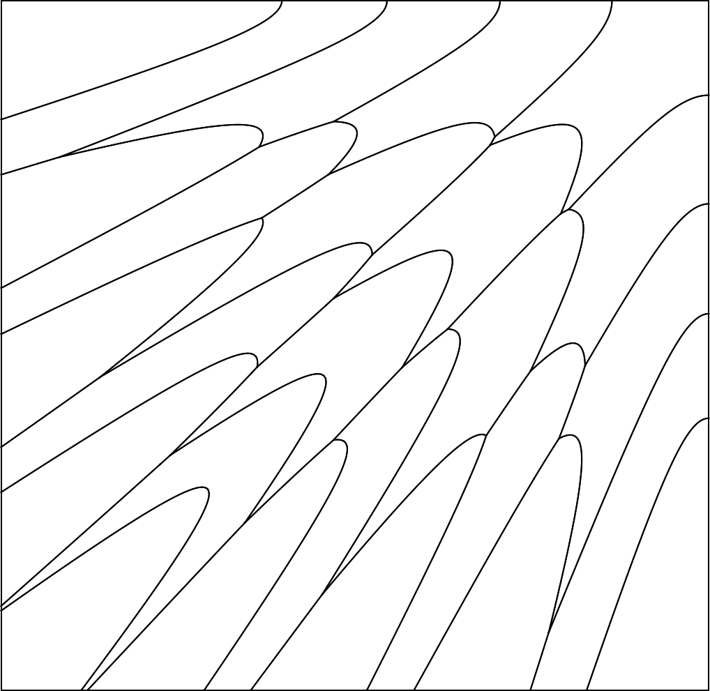
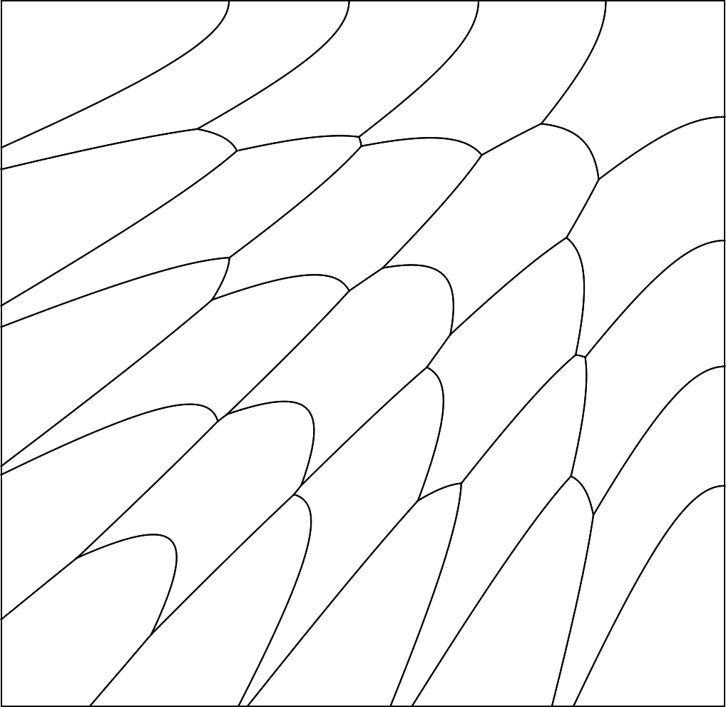
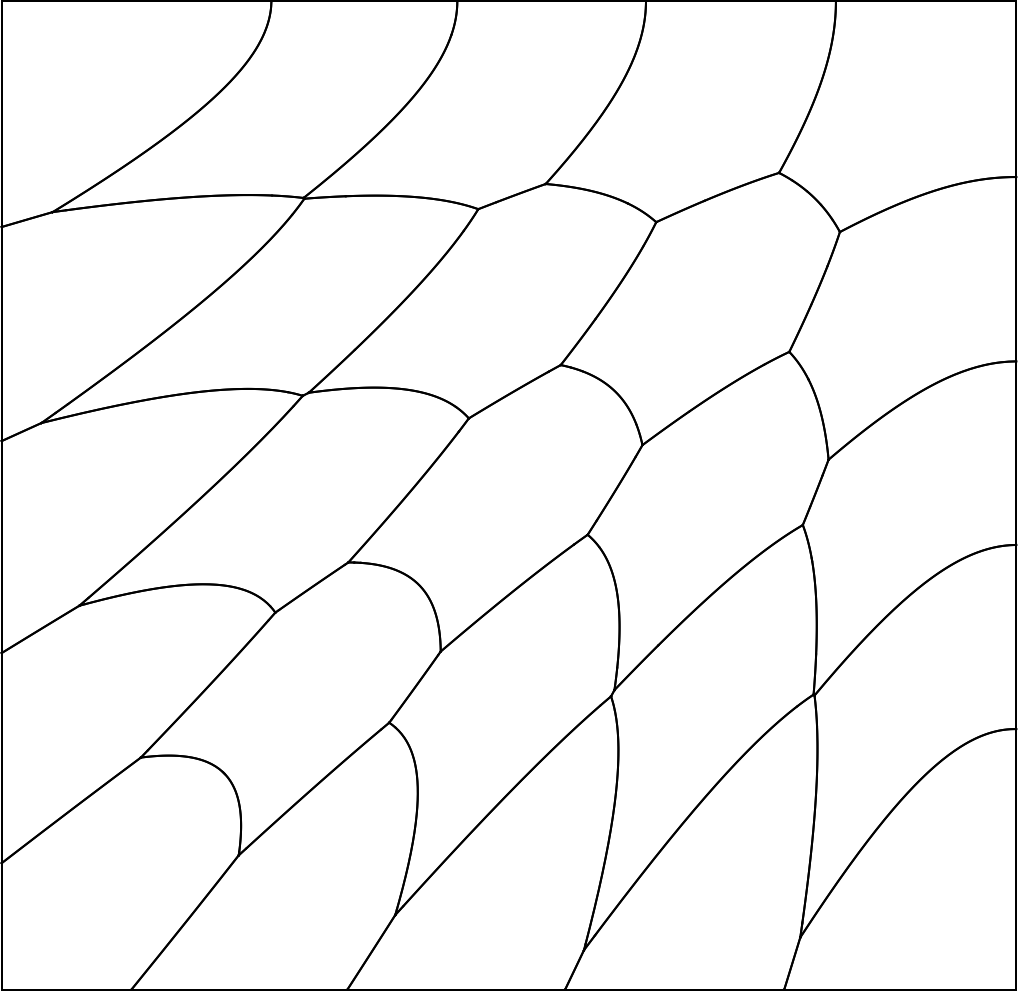
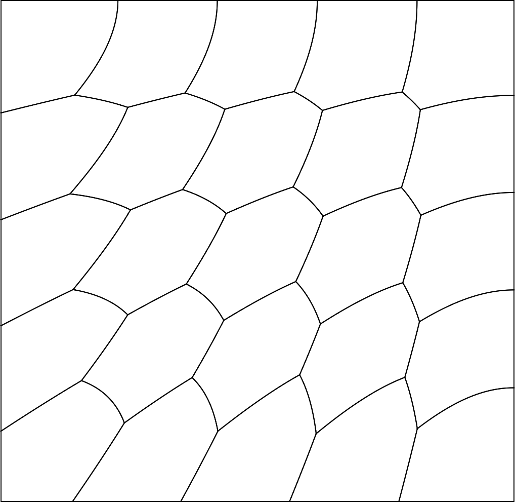
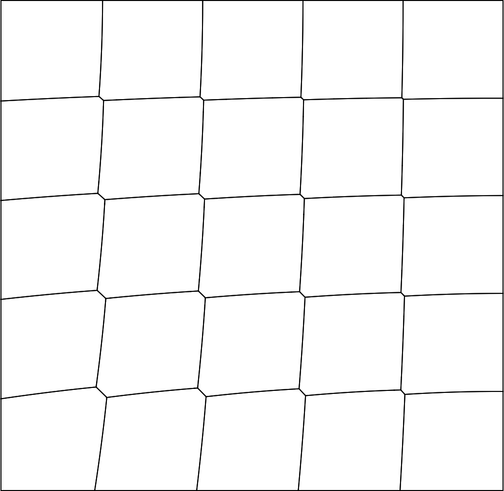
Computing the Laguerre cells associated to the near-field refractor metasurface problem is not an easy task, because these cells have curved boundaries (see Figure 1), are not convex, etc. In this section, we show that the Laguerre cells can be obtained by using power diagrams. The advantage of this formulation is that there are very efficient algorithms and software libraries available to construct 3D power diagrams, with near-linear complexity in $N$ for non-degenerate input.

Definition 4.2.

Let $Q=\{(q_{i},\omega_{i})\}_{1\leq i\leq N}$ be a weighted cloud point set, i.e., $q_{i}\in{\mathbb{R}}^{3}$ and $\omega_{i}\in{\mathbb{R}}$. Then for each $1\leq i\leq N$, the $i$-th power diagram of $Q$ is defined by

$$\text{Pow}_{i}(Q)=\left\{x\in{\mathbb{R}}^{3}:|x-q_{i}|^{2}+\omega_{i}\leq|x-q_{j}|^{2}+\omega_{j}\quad\forall j\in\{1,\cdots,N\}\right\}.$$

Let us define

$$H_{i}({\bf b})=\left\{X\in{\mathbb{R}}^{2}\times\{\alpha\}:|X-Y_{i}|+b_{i}\leq|X-Y_{j}|+b_{j},\quad\forall 1\leq j\leq N\right\},\quad 1\leq i\leq N,$$

with ${\bf b}=\left(b_{1},\cdots,b_{N}\right)$, $0<\alpha<\beta$, and the points $Y_{i}=(y_{i},\beta)$ lie in the horizontal plane ${\mathbb{R}}^{2}\times\{\beta\}$. From the definition of Laguerre cell in (3.1), we have

$$\text{Lag}_{i}({\bf b})=H_{i}({\bf b})\cap\Omega.$$

Proposition 4.3 (Point Source/Near-Field).

We assume the following condition

(4.2) $$\forall i,j\in\{1,\cdots,N\}\quad|b_{i}-b_{j}|<\sqrt{4(\alpha-\beta)^{2}+|y_{i}-y_{j}|^{2}}.$$

Then, for each $i\in\{1,\cdots,N\}$, one has

$$H_{i}({\bf b})=\text{P}_{{\mathbb{R}}^{2}\times\{\alpha\}}\left(\text{Pow}_{i}(Q)\cap\Sigma_{i}^{+}\right)$$

where $\text{P}_{{\mathbb{R}}^{2}\times\{\alpha\}}$ denotes the orthogonal projection onto ${\mathbb{R}}^{2}\times\{\alpha\}$, $Q=\{(q_{i},\omega_{i})\}_{i=1}^{N}$ is the weighted point cloud with $q_{i}=(y_{i},-b_{i})$ and $\omega_{i}=-2\,b_{i}^{2}$, and where $\Sigma_{i}^{+}$ is one sheet of a hyperboloid given by $\Sigma_{i}^{+}=\left\{\left(x,|X-Y_{i}|+b_{i}\right):X=(x,\alpha),x\in{\mathbb{R}}^{2}\right\}$. Therefore,

$$\text{Lag}_{i}({\bf b})=\text{P}_{{\mathbb{R}}^{2}\times\{\alpha\}}\left(\text{Pow}_{i}(Q)\cap\Sigma_{i}^{+}\cap\Omega\right).$$

In practice, condition (4.2) is not restrictive because to use the damped Newton algorithm from Section 4.1, one needs to assume that the Laguerre cells at the initialization vector ${\bf b}^{0}$ are non empty which by the corollary below implies (4.2).

Corollary 4.4.

If the vector ${\bf b}$ satisfies $\text{Lag}_{i}({\bf b})\neq\emptyset$ for each $1\leq i\leq N$, then

$$\text{Lag}_{i}({\bf b})=\text{P}_{{\mathbb{R}}^{2}\times\{\alpha\}}\left(\text{Pow}_{i}(Q)\cap\Sigma_{i}^{+}\cap\Omega\right),$$

for all $1\leq i\leq N$.

Proof.

Fix $1\leq i,j\leq N$ with $i\neq j$ and suppose that ${\bf b}=(b_{1},\cdots,b_{N})$ is such that $\text{Lag}_{i}({\bf b})\neq\emptyset$ and $\text{Lag}_{j}({\bf b})\neq\emptyset$ contain points $X_{i}$ and $X_{j}$ respectively. Then,

$$|X_{i}|+|X_{i}-Y_{i}|=c(X_{i},Y_{i})+b_{i}\leq c(X_{i},Y_{j})+b_{j}=|X_{i}|+|X_{i}-Y_{j}|+b_{j}.$$

Thus, $b_{i}-b_{j}\leq|Y_{i}-Y_{j}|=|y_{i}-y_{j}|$. By symmetry, we get

$$|b_{i}-b_{j}|\leq|y_{i}-y_{j}|<\sqrt{4(\alpha-\beta)^{2}+|y_{i}-y_{j}|^{2}}.\qed$$

Remark 4.5.

If $\alpha=\beta$, then the Laguerre diagram is known as Apollonius diagram where all the surfaces $\Sigma_{i}^{+}$ are half-cones. When $\alpha\neq\beta$, then each $\Sigma_{i}^{+}$ is not anymore a cone but a sheet of a hyperboloid.

Remark 4.6 (Initialization).

To apply the algorithm from Section 4.1, we need to find an initial vector ${\bf b}^{0}=(b_{1},\cdots,b_{N})$ for which the corresponding Laguerre cells are not empty. Taking ${\bf b}^{0}=0$ this is the case when

$$\text{P}_{{\mathbb{R}}^{2}\times\{\alpha\}}(Y_{i})\in\Omega,\forall i\in\{1,\cdots,N\}.$$

Indeed, if we denote by $X_{i}=(y_{i},\alpha)$ such a point, we see that $|X_{i}-Y_{i}|=|\beta-\alpha|\leq|X_{i}-Y_{j}|$ for any $j$, implying that $X_{i}\in\text{Lag}_{i}(0)$. For other options to choose the initialization vector see [Mey19, Sec. 2.3].

4.3. Proof of Proposition 4.3

Let us consider the hyperboloid of two sheets

$$\Sigma_{i}=\left\{(x,x_{3}):|X-Y_{i}|^{2}=(x_{3}-b_{i})^{2},X=(x,\alpha),x\in{\mathbb{R}}^{2}\right\}$$

with $Y_{i}=(y_{i},\beta)$, $\beta>\alpha$. The upper sheet of this hyperboloid is given parametrically by

$$\Sigma_{i}^{+}=\left\{\left(x,|X-Y_{i}|+b_{i}\right):X=(x,\alpha),x\in{\mathbb{R}}^{2}\right\}$$

and the lower sheet is given by

$$\Sigma_{i}^{-}=\left\{\left(x,-|X-Y_{i}|+b_{i}\right):X=(x,\alpha),x\in{\mathbb{R}}^{2}\right\}.$$

Clearly, $\Sigma_{i}^{-}$ and $\Sigma_{i}^{+}$ are symmetric with respect to the hyperplane $\{x_{3}=b_{i}\}$, and $\Sigma_{i}=\Sigma_{i}^{-}\cup\Sigma_{i}^{+}$.

We first need to determine the relative positions of the hyperboloids $\Sigma_{i}$ and $\Sigma_{j}$.

Lemma 4.7.

We have the following:

1. If $\Sigma_{i}^{+}\cap\Sigma_{j}^{-}=\emptyset$, then $\Sigma_{i}^{+}$ is strictly above $\Sigma_{j}^{-}$, i.e., for any $x\in{\mathbb{R}}^{2}$ such that $(x,x_{3}^{i})\in\Sigma_{i}^{+}$ and $(x,x_{3}^{j})\in\Sigma_{j}^{-}$, one has $x_{3}^{i}>x_{3}^{j}$.

2. $\sqrt{4(\alpha-\beta)^{2}+|y_{i}-y_{j}|^{2}}>b_{j}-b_{i}$ if and only if $\Sigma_{i}^{+}\cap\Sigma_{j}^{-}=\emptyset$.

3. If $\Sigma_{i}^{+}\cap\Sigma_{j}^{-}\neq\emptyset$, then $\Sigma_{i}^{+}$ is strictly below $\Sigma_{j}^{+}$, i.e., for any $x\in{\mathbb{R}}^{2}$ such that $(x,x_{3}^{i})\in\Sigma_{i}^{+}$ and $(x,x_{3}^{j})\in\Sigma_{j}^{+}$, one has $x_{3}^{i}<x_{3}^{j}$.

Proof.

(1) Since $\Sigma_{i}^{+}$ opens upwards and $\Sigma_{j}^{-}$ opens downwards, if they don’t intersect, it is clear that $\Sigma_{i}^{+}$ must be strictly above $\Sigma_{j}-$.

(2) We have $\Sigma_{i}^{+}\cap\Sigma_{j}^{-}\neq\emptyset$ iff there exists $X\in{\mathbb{R}}^{2}\times\{\alpha\}$ with

$$|X-Y_{i}|+|Y_{j}-X|=b_{j}-b_{i}.$$

On the other hand, for each $X\in{\mathbb{R}}^{2}\times\{\alpha\}$, one has

$$|X-Y_{i}|+|Y_{j}-X|\geq|X_{i,j}-Y_{i}|+|X_{i,j}-Y_{j}|=2\sqrt{(\alpha-\beta)^{2}+|y_{i}-y_{j}|^{2}/4},$$

where $X_{i,j}=((y_{i}+y_{j})/2,\alpha)$. Therefore, $\sqrt{4(\alpha-\beta)^{2}+|y_{i}-y_{j}|^{2}}>b_{j}-b_{i}$ implies $\Sigma_{i}^{+}\cap\Sigma_{j}^{-}=\emptyset$.

Vice versa, from Item (1), $|X-Y_{i}|+b_{i}>-|X-y_{j}|+b_{j}$ for each $X=(x,\alpha)$ and so $b_{j}-b_{i}$ satisfies the desired inequality.

(3) By contradiction. Suppose there are points $(x,x_{3}^{i})\in\Sigma_{i}^{+}$ and $(x,x_{3}^{j})\in\Sigma_{j}^{+}$ with $x_{3}^{i}\geq x_{3}^{j}$. If $X=(x,\alpha)$, then $|X-Y_{i}|+b_{i}=x_{3}^{i}\geq x^{3}_{j}=|X-Y_{j}|+b_{j},$ and so $b_{j}-b_{i}\leq|Y_{i}-Y_{j}|$ from triangle inequality. Now, $\sqrt{4(\alpha-\beta)^{2}+|y_{i}-y_{j}|^{2}}\leq b_{j}-b_{i}$ from (2). Since $|Y_{i}-Y_{j}|<\sqrt{4(\alpha-\beta)^{2}+|y_{i}-y_{j}|^{2}}$, we obtain a contradiction.

∎

The previous lemma leads to the following.

Lemma 4.8.

Fix $i,j$ and define the sets

$$L_{i,j}^{\leq}:=\left\{X\in{\mathbb{R}}^{2}\times\{\alpha\}:|X-Y_{i}|+b_{i}\leq|X-Y_{j}|+b_{j}\right\}\supset\text{Lag}_{i}({\bf b}),$$

$$H_{ij}^{\leq}:=\left\{x\in{\mathbb{R}}^{3}:|x-q_{i}|^{2}+\omega_{i}\leq|x-q_{j}|^{2}+\omega_{j}\right\},\quad\omega_{j}=-2\,b_{j}^{2};\quad q_{j}=(y_{j},-b_{j}).$$

We have:

1. If $\sqrt{4(\alpha-\beta)^{2}+|y_{i}-y_{j}|^{2}}>b_{j}-b_{i}$, then

   $$L_{i,j}^{\leq}=\text{P}_{{\mathbb{R}}^{2}\times\{\alpha\}}\left(H_{ij}^{\leq}\cap\Sigma_{i}^{+}\right)$$

2. If $\sqrt{4(\alpha-\beta)^{2}+|y_{i}-y_{j}|^{2}}\leq b_{j}-b_{i}$, then $L_{i,j}^{\leq}={\mathbb{R}}^{2}\times\{\alpha\}$.

Proof.

(1) Let $X=(x,\alpha)\in L_{i,j}^{\leq}$, and $x_{3}=|X-Y_{i}|+b_{i}$. By Lemma 4.7 (2) and (1), the point $(x,x_{3})\in\Sigma_{i}^{+}$ is above $\Sigma_{j}^{-}$, and so $x_{3}-b_{j}>-|Y_{j}-X|$. By definition of $L_{i,j}^{\leq}$, we also have $x_{3}-b_{j}\leq|Y_{j}-X|$, which implies

$$(x_{3}-b_{i})^{2}=|X-Y_{i}|^{2}\quad\mbox{and}\quad(x_{3}-b_{j})^{2}\leq|X-Y_{j}|^{2}.$$

Expanding these two equations, one gets

$$\left\{\begin{array}[]{l}x_{3}^{2}-2b_{i}x_{3}+b_{i}^{2}=|X|^{2}-2X\cdot Y_{i}+|Y_{i}|^{2}\\ x_{3}^{2}-2b_{j}x_{3}+b_{j}^{2}\leq|X|^{2}-2X\cdot Y_{j}+|Y_{j}|^{2}.\\ \end{array}\right.\\$$

Subtracting the first line from the second line yields

$$-2(x,x_{3})\cdot(y_{i},-b_{i})+|Y_{i}|^{2}-b_{i}^{2}\leq-2(x,x_{3})\cdot(y_{j},-b_{j})+|Y_{j}|^{2}-b_{j}^{2}$$

which can be rewritten as

$$|(x,x_{3})-(y_{i},-b_{i})|^{2}-2b_{i}^{2}\leq|(x,x_{3})-(y_{j},-b_{j})|^{2}-2b_{j}^{2}.$$

This means $(x,x_{3})\in H_{ij}^{\leq}$ and so $(x,x_{3})\in H_{ij}^{\leq}\cap\Sigma_{i}^{+}$. To show the opposite inclusion, let $(x,x_{3})\in H_{ij}^{\leq}\cap\Sigma_{i}^{+}$ and put $X=(x,\alpha)$. Then one has

$$\left\{\begin{array}[]{l}x_{3}=|X-Y_{i}|+b_{i}\\ |(x,x_{3})-(y_{i},-b_{i})|^{2}-2b_{i}^{2}\leq|(x,x_{3})-(y_{j},-b_{j})|^{2}-2b_{j}^{2}.\end{array}\right.\\$$

Reversing the previous calculation, one gets $(x_{3}-b_{j})^{2}\leq|X-Y_{j}|^{2}$. This obviously implies $-|X-Y_{j}|\leq x_{3}-b_{j}\leq|X-Y_{j}|$, which gives in particular that $X\in L_{i,j}^{\leq}$, completing the proof of (1).

(2) From Lemma 4.7 (2), $\Sigma_{i}^{+}\cap\Sigma_{j}^{-}\neq\emptyset$ and so from Item (3) in that lemma, $\Sigma_{i}^{+}$ is strictly below $\Sigma_{j}^{+}$. That is, $b_{i}+|X-Y_{i}|<b_{j}+|X-Y_{j}|$ for all $x\in{\mathbb{R}}^{2}$, $X=(x,\alpha)$. This means $L_{i,j}^{\leq}$ is the whole plane ${\mathbb{R}}^{2}\times\{\alpha\}$. ∎

Proof of Proposition 4.3.

Let $i\in\{1,\cdots,N\}$. From (4.2) we can apply Lemma 4.8(1) to obtain

$$H_{i}({\bf b})=\displaystyle\bigcap_{1\leq j\leq N}L_{i,j}^{\leq}=\bigcap_{1\leq j\leq N}\text{P}_{{\mathbb{R}}^{2}\times\{\alpha\}}\left(H_{ij}^{\leq}\cap\Sigma_{i}^{+}\right)=\text{P}_{{\mathbb{R}}^{2}\times\{\alpha\}}\left(\Sigma_{i}^{+}\cap\bigcap_{1\leq j\leq N}H_{ij}^{\leq}\right)$$

Since by definition $\text{Pow}_{i}(Q)=\bigcap_{1\leq j\leq N}H_{ij}^{\leq}$, the proposition follows. ∎

4.4. Numerical experiments

In all three numerical experiments, we assume that the source measure $\rho\equiv\frac{1}{4}$ is uniform over the square $\Omega=[-1,1]^{2}\times\{\alpha\}$, and we also assume that the metasurface is at height $\alpha=1$. The Laguerre cells are computed using Proposition 4.3, by intersecting 3D power cells with a quadric. To describe the algorithm, we use the notation from that proposition:

• First, we compute 3D the power diagram $(\text{Pow}_{i}(Q))_{1\leq i\leq N}$ using the CGAL library and we restrict each cell to the lifted domain $\Omega\times{\mathbb{R}}$ by computing the intersection $P_{i}=\text{Pow}_{i}(Q)\cap(\Omega\times{\mathbb{R}})$. In the implementation, we assume that $\Omega\subseteq{\mathbb{R}}^{2}$ is a convex polygon.

• For every pair $i\neq j\in\{1,\ldots,N\}$, we compute the curve $\gamma_{ij}$ corresponding to the projection on ${\mathbb{R}}^{2}\times\{\alpha\}$ of the facet $P_{i}\cap P_{j}$ with the quadric $\Sigma_{i}^{+}$,

  $$\gamma_{ij}=\text{P}_{{\mathbb{R}}^{2}\times\{\alpha\}}(P_{i}\cap P_{j}\cap\Sigma_{i}^{+}).$$

  In practice, we need to make this computation only if the power cells already have a non-empty interface, i.e. if $P_{i}\cap P_{j}\neq\emptyset$. We also note that by Proposition 4.3,

  $$\text{Lag}_{i}({\bf b})\cap\text{Lag}_{j}({\bf b})=\gamma_{ij}.$$

• We finally compute the intersection of each Laguerre cell with the boundary of the domain using the formula

  $$\gamma_{i,\infty}=\text{Lag}_{i}({\bf b})\cap\Omega=\text{P}_{{\mathbb{R}}^{2}\times\{\alpha\}}(\text{Pow}_{i}(Q)\cap\partial\Omega).$$

By construction, the boundary of the $i$th Laguerre cell is given by

$$\partial\text{Lag}_{i}({\bf b})=\gamma_{i,\infty}\cup\bigcup_{j\neq i}\gamma_{ij},$$

and the union is disjoint up to a finite set, which is negligible. We may then use this description of the boundary of the cell $\text{Lag}_{i}({\bf b})$ to compute the integral of $\rho$ over $\text{Lag}_{i}({\bf b})$ using divergence theorem

$$G_{i}({\bf b})=\int_{\text{Lag}_{i}({\bf b})}\rho(X)dX=\frac{1}{8}\int_{\partial\text{Lag}_{i}({\bf b})}X\cdot n_{i}(X)dX,$$

where $n_{i}$ denotes the exterior normal to $\text{Lag}_{i}({\bf b})$, and where the second integral is 1-D. The partial derivatives are computed using (3.4): for $i\neq j$ we have

$$\dfrac{\partial G_{i}}{\partial b_{j}}({\bf b})=\int_{\gamma_{ij}}\dfrac{1}{4}\dfrac{1}{\left|\nabla_{X}c(X,Y_{i})-\nabla_{X}c(X,Y_{j})\right|}\,dX,$$

where again the integrals are one dimensional. The code to compute the intersection between the power cell $\text{Pow}_{i}(Q)$ and the quadric $\Sigma_{i}^{+}$ and to perform the numerical integration is written in a combination of C++ and Python, and is available online, as well as the experiments presented below.

4.4.1. Effect of changes in $\beta-\alpha$ on the shape of $\text{Lag}_{i}({\bf b})$

In the first numerical experiment, we study the effect of the distance between the metasurface and the target, $\delta=\beta-\alpha$, on the shape of the Laguerre cells. We assume that the target is of the form

$$\nu=\frac{1}{N}\sum_{1\leq i\leq 25}\delta_{y_{i}},$$

where $N=25$ and $\{y_{1},\ldots,y_{N}\}$ is a uniform $5\times 5$ grid contained in the square $[0,1]^{2}$, and we solve the optimal transport problem between $\rho$ and $\nu$. Our goal in this first experiment is to visualize the effect of changes in $\delta$, the vertical distance between the source and the metasurface, on the shape of the solution. We initialize the damped Newton algorithm described in Section 4.1 with ${\bf b}^{0}=(0,\ldots,0)$. The associated Laguerre cells coincides with the Voronoi cells of the point cloud $\{Y_{1},\ldots,Y_{N}\}$, i.e.

$$\mathrm{Vor}_{i}=\{X\in{\mathbb{R}}^{2}\times\{\alpha\}\mid\forall j\in\{1,\ldots,N\},~{}|{X-Y_{i}}|\leq|{X-Y_{j}}|\}.$$

and is shown on the first row and column of Figure 1. We solve the near-field metasurface problem for several values of $\delta$, and we display the Laguerre cells of the solution. In particular, one can see that for $\delta=2$, the solution is very similar to the solution of the optimal transport problem for the “standard” quadratic cost.

4.4.2. Convergence speed

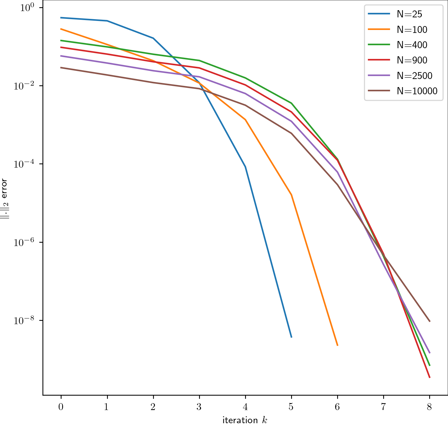
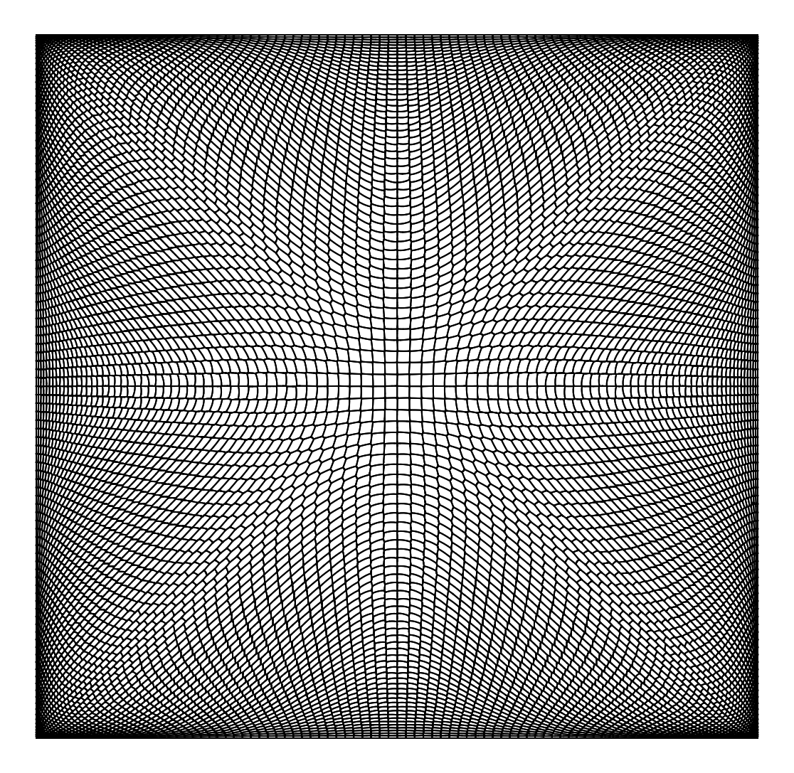
In our second numerical experiment, the target measure $\nu$ approximates the restriction of the Gaussian $e^{-2|{\cdot}|^{2}}$ to the unit square $[-1,1]^{2}\times\{\alpha\}$. More precisely, the measure $\nu$ is of the form

$$\nu=\frac{1}{N}\sum_{1\leq i\leq N}\nu_{i}\delta_{y_{i}},$$

where $N=n^{2}$ and $n\in\{5,10,20,30,40,50,100\}$. The points $\{y_{1},\ldots,y_{N}\}$ form a uniform $n\times n$ grid in the square $[-1,1]^{2}\times\{\alpha\}$. The mass $\nu_{i}$ of the Dirac $\delta_{y_{i}}$ is defined by evaluating a Gaussian at $y_{i}$:

$$\nu_{i}=e^{-2|{y_{i}}|^{2}}/\sum_{1\leq j\leq N}e^{-2|{y_{j}}|^{2}}.$$

Figure 3 displays the solution of this problem for $N=100^{2}$. Figure 2 displays the decrease of the numerical error along the iterations of the algorithm, defined as

$$\varepsilon_{k}=\left(\sum_{i}(H_{i}({\bf b}^{k})-\nu_{i})^{2}\right)^{1/2},$$

for several values of $N$. In particular, one can see from this figure that a numerical error of $10^{-8}$ is reached in less than 8 iterations, even for $N=10^{4}$.

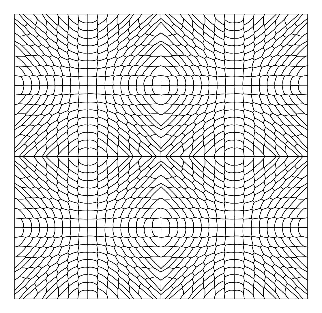
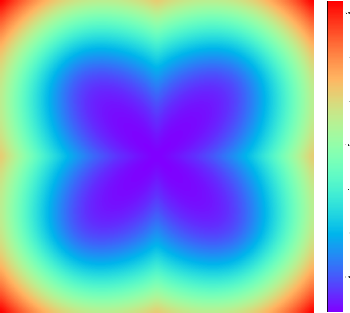
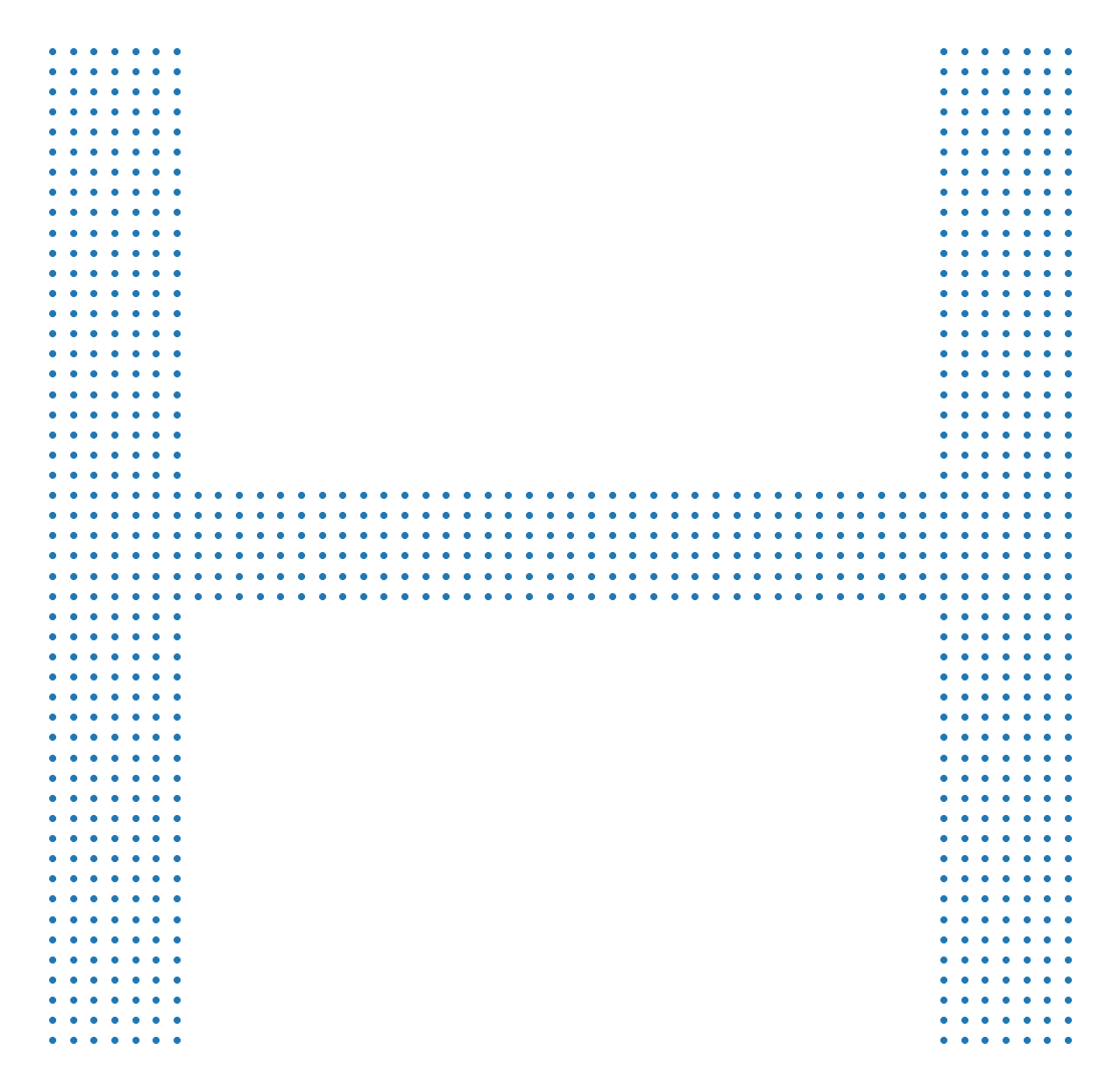
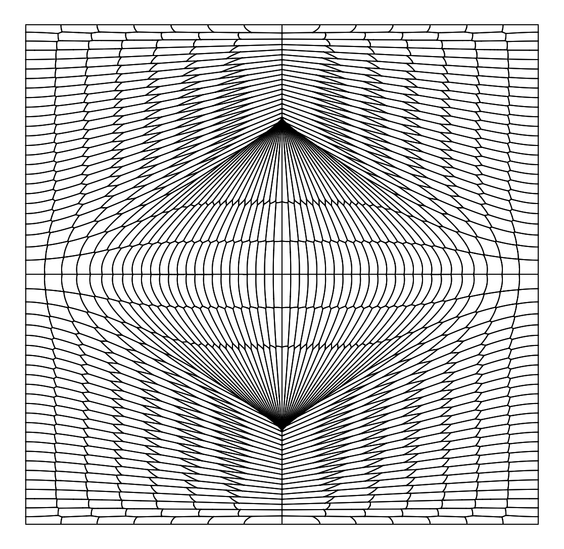
4.4.3. Visualization of the phase

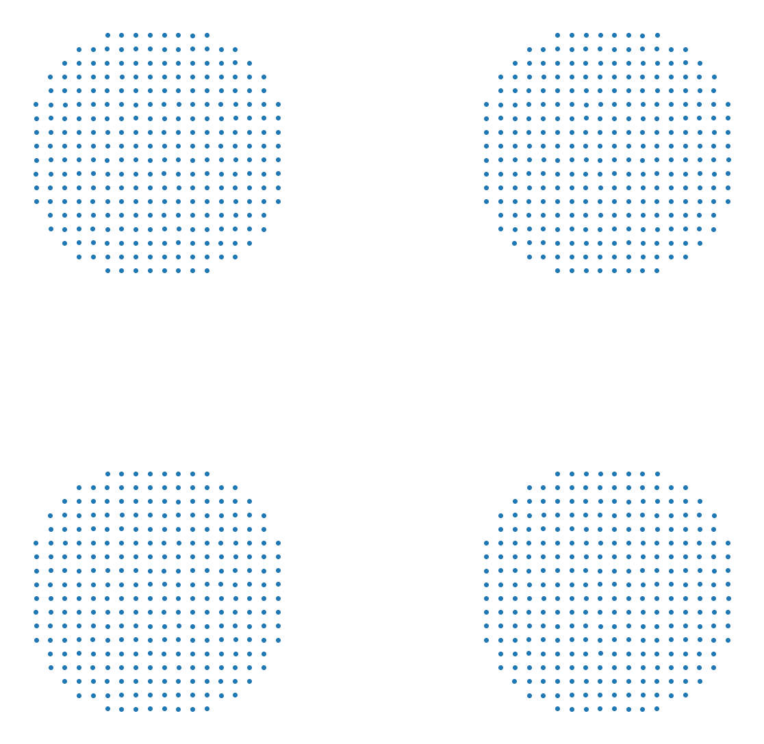
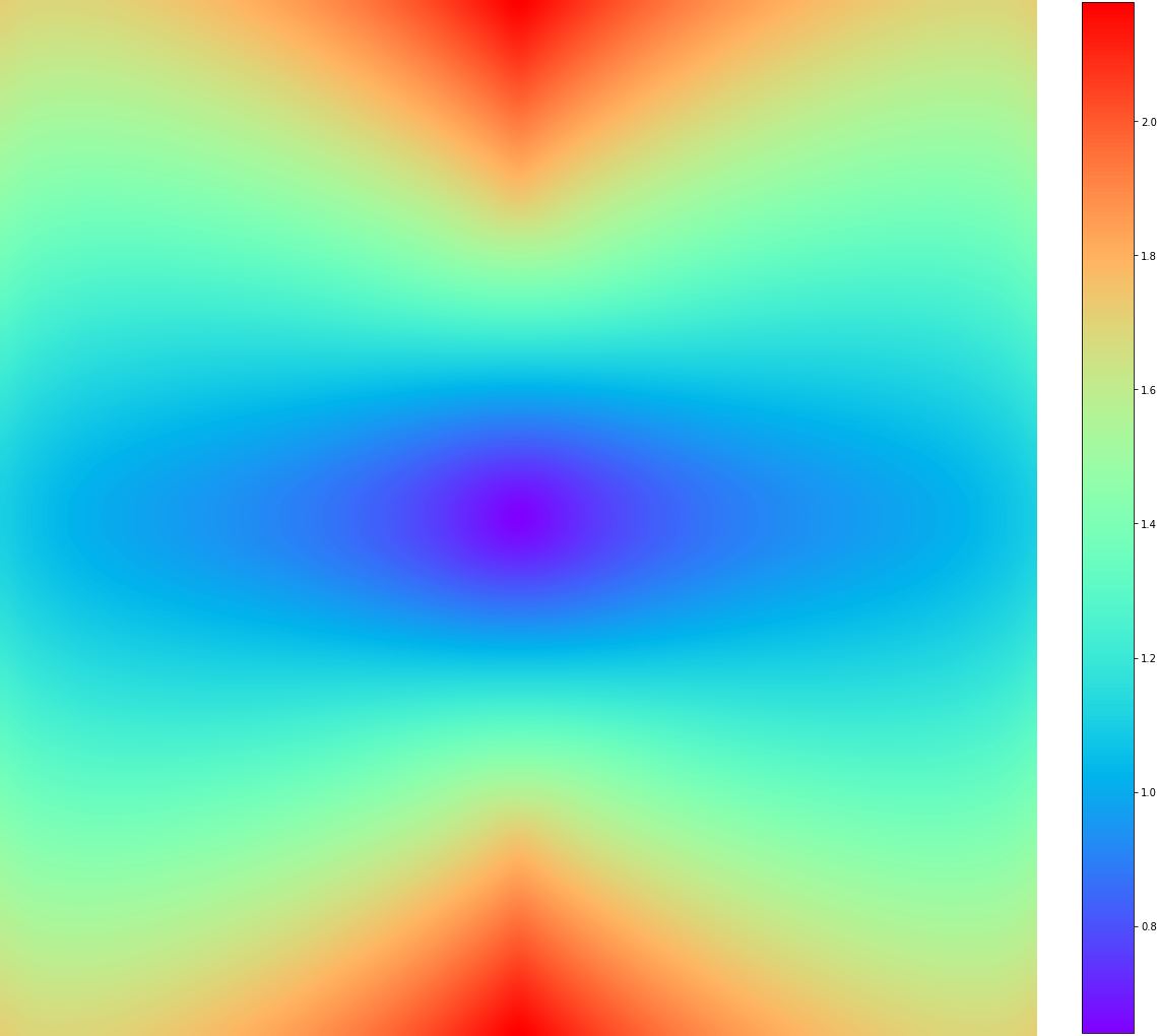
In this last numerical experiment, the target is uniform over four discretized disks (Figure 4, top row) or over a discretized letter H (Figure 4, bottom row), i.e. $\nu\equiv 4/N$ where $N$ is the number of points composing the discretized shapes. Figure 4 displays the Laguerre cells corresponding to the solution of the near-field metasurface problem. We also display the corresponding phase discontinuity $\phi$, which can be computed thanks to Theorem 2.3. On the “four disks” example, one may notice that the gradient of the phase discontinuity $\phi$ seems to exhibit a discontinuity on the “cross” $\{0\}\times[0,1]\times\{\alpha\}\cup[0,1]\times\{0\}\times\{\alpha\}$: this corresponds to a jump in the transport map which is necessary to cross the void between the four disks.

Figure 1. From left to right and top to bottom: The first image displays the Voronoi cells of $\{Y_{1},\ldots,Y_{N}\}$. Then, each image displays the Laguerre cells associated to the solutions of the near-field metasurface problem described in §4.4.1 for $\delta\in\{0.1,0.2,0.3,0.5,2\}$.

Figure 2. Convergence of the numerical error in terms of the iteration number for the near-field metasurface problem described in §4.4.2, for $N\in\{5,10,20,30,40,50,100\}^{2}$.

Figure 3. Laguerre diagram associated to the solution of the near-field metasurface problem described in §4.4.2, for $N=100^{2}$.

Figure 4. Near-field metasurface with a target measure supported over four discretized disks (top) or a discretized letter H (bottom): Support of the target measure (left), Laguerre cells associated to the solution (middle), and the corresponding phase discontinuity $\phi$ (right).

5. Refraction into the far field

We consider here the case when incident rays emanate in a collimated beam and the case when they emanate from a point source. Since the arguments to treat these problems are similar to the ones used in Section 2, we only indicate the modifications that are needed.

5.1. Collimated beam

Let $\Gamma$ be the horizontal plane $x_{3}=a$ in ${\mathbb{R}}^{3}$, ${\bf e}=(0,0,1)$. The phase discontinuity function $\phi(x)$ with $x=(x_{1},x_{2},x_{3})$ defined in a neighborhood of $\Gamma$ such that the metasurface $(\Gamma,\phi)$ refracts all vertical rays having direction ${\bf e}$ into a fixed unit direction ${\bf m}=\left(m_{1},m_{2},m_{3}\right)$, with $m_{3}>0$, is given by

$$\phi(x)={\bf v}\cdot x,\text{ with }{\bf v}=({\bf m}\cdot{\bf e})\,{\bf e}-{\bf m}=\left(-m_{1},-m_{2},0\right);$$

see [GS21, Theorem 4.1] for a proof in the more general case when ${\bf m}$ is a variable set of directions depending on $x$. Notice that if ${\bf m}=\left(m_{1},m_{2},m_{3}\right)$ and ${\bf m}^{\prime}=\left(m_{1}^{\prime},m_{2}^{\prime},m_{3}^{\prime}\right)$ are two unit vectors with $m_{3},m_{3}^{\prime}>0$ and $\left(m_{1},m_{2}\right)=\left(m_{1}^{\prime},m_{2}^{\prime}\right)$, then ${\bf m}={\bf m}^{\prime}$.

Each vector ${\bf m}=\left(m_{1},m_{2},m_{3}\right)\in S^{2}$ with $m_{3}>0$ can be identified with its projection $\left(m_{1},m_{2}\right)$ on the disk of radius one around $(0,0)$ where $m_{3}=\sqrt{1-m_{1}^{2}-m_{2}^{2}}$.

Fix a compact region $\Omega\subset\Gamma$ with points $x=(x_{1},x_{2},a)$ and a compact region $\Omega^{*}\subset S^{2}_{+}$.

Definition 5.1 (Admissible phase).

The function $\phi:\Omega\to{\mathbb{R}}$ is an admissible phase refracting $\Omega$ into $\Omega^{*}$ if for each $x_{0}\in\Omega$ there exists ${\bf m}\in\Omega^{*}$ and $b\in{\mathbb{R}}$ such that

$$\phi(x) \geq b+\left(({\bf m}\cdot{\bf e})\,{\bf e}-{\bf m}\right)\cdot x:=L({\bf m},b,x),\qquad\forall x\in\Omega,\text{ and}$$

$$\phi(x_{0}) =b+\left(({\bf m}\cdot{\bf e})\,{\bf e}-{\bf m}\right)\cdot x_{0}.$$

We say that $L({\bf m},b,x)$ is a supporting phase to $\phi$ at $x_{0}$.

Definition 5.2.

Given $x_{0}\in\Omega$ and $\phi$ an admissible phase, we define the set-valued mapping $\mathcal{N}_{\phi}:\Omega\to\mathcal{P}(\Omega^{*})$ given by

$$\mathcal{N}_{\phi}(x_{0})=\{m\in\Omega^{*}:\text{there exists $b\in{\mathbb{R}}$ such that $L({\bf m},b,x)$ is a supporting phase to $\phi$ at $x_{0}$}\};$$

and the inverse map

$$\left(\mathcal{N}_{\phi}\right)^{-1}(m)=\{x\in\Omega:m\in\mathcal{N}_{\phi}(x)\}.$$

Define the class

$$\mathcal{F}=\{\phi:\Omega\to{\mathbb{R}}:\text{$\phi$ is an admissible phase refracting $\Omega$ into $\Omega^{*}$}\}.$$

Given $f\in L^{1}(\Omega)$, non negative, assuming that $\partial\Omega$ has 2-dimensional Lebesgue measure zero, and given a Borel measure $\mu$ in $\Omega^{*}$ satisfying $\int_{\Omega}f(x)\,dx=\mu(\Omega^{*}),$ our problem is then to find $\phi\in\mathcal{F}$ solving

(5.1) $$\mathcal{M}_{\phi}(E):=\int_{(\mathcal{N}_{\phi})^{-1}(E)}f(x)\,dx=\mu(E)$$

for each Borel set $E\subset\Omega^{*}$. To show existence and uniqueness to this problem, we proceed as in Section 2 with the following changes. The class $\mathcal{F}$ satisfies the following properties that follow immediately from the definitions above

1. If $\phi_{1},\phi_{2}\in\mathcal{F}$, then $\phi_{1}\vee\phi_{2}=\max\{\phi_{1},\phi_{2}\}\in\mathcal{F}$,

2. if $\phi_{1}(x_{0})\geq\phi_{2}(x_{0})$, then $\mathcal{N}_{\phi_{1}}(x_{0})\subset\mathcal{N}_{\phi_{1}\vee\phi_{2}}(x_{0})$,

3. Given ${\bf m}\in\Omega^{*}$ the functions $L({\bf m},b,x)\in\mathcal{F}$, $b\in(-\infty,\infty)$, satisfy the following

   1. ${\bf m}\in\mathcal{N}_{L({\bf m},b,x)}(x)$ for all $x\in\Omega$,

   2. $L({\bf m},b,x)\leq L({\bf m},b^{\prime},x)$ for all $b\leq b^{\prime}$,

   3. for each ${\bf m}\in\Omega^{*}$, $L({\bf m},b,x)\to+\infty$ uniformly for $x\in\Omega$ as $b\to+\infty$,

   4. for each ${\bf m}\in\Omega^{*}$, $\max_{x\in\Omega}|L({\bf m},b^{\prime},x)-L({\bf m},b,x)|\to 0$ as $b^{\prime}\to b$.

Recalling the notation at the beginning of Section 2.3, we now let ${\mathcal{X}}=\Omega$ and ${\mathcal{Y}}=\Omega^{*}$, and with similar arguments but now using conditions $(A1)^{\prime}-(A3)^{\prime}$ instead of $(A1),(A2),(A3)^{\prime\prime}$, we get that $\mathcal{N}_{\phi}\in C_{s}(\Omega,\Omega^{*})$ for each $\phi\in\mathcal{F}$. Then to prove existence and uniqueness when $\mu=\sum_{i=1}^{N}g_{i}\,\delta_{{\bf m}_{i}}$, we use [GH14, Theorem 2.12], for which we only need to verify its hypotheses. In fact, we need to verify that there exist numbers $b_{1}^{0},\cdots,b_{N}^{0}$ such that the admissible phase $\phi_{0}(x)=\max_{1\leq i\leq N}L\left({\bf m}_{i},b_{i}^{0},x\right)$, for $x\in\Omega$, satisfies $\mathcal{M}_{\phi_{0}}({\bf m}_{j})\leq g_{j}$ for $2\leq j\leq N$. By continuity, given any $b_{1}^{0}$ we can pick $b_{2}^{0},\cdots,b_{N}^{0}$ tending to $-\infty$ such that $L\left({\bf m}_{i},b_{i}^{0},x\right)<L\left({\bf m}_{1},b_{1}^{0},x\right)$ for all $i\neq 1$ and $x\in\Omega$. Therefore, $\phi_{0}(x)=L\left({\bf m}_{1},b_{1}^{0},x\right)$. Since the points ${\bf m}_{i}=\left(m_{1}^{i},m_{2}^{i},m_{3}^{i}\right)\neq{\bf m}_{j}=\left(m_{1}^{j},m_{2}^{j},m_{3}^{j}\right)$ for $i\neq j$, the family of planes having equations $z=\alpha-m_{1}^{i}\,x_{1}-m_{2}^{i}\,x_{2}$ are never parallel. Consequently, $\mathcal{N}_{\phi_{0}}({\bf m}_{i})\subset\partial\Omega$ for $i\neq 1$ and so $\mathcal{M}_{\phi_{0}}({\bf m}_{i})=0$ for $i\neq 1$. The hypotheses in [GH14, Theorem 2.12] then hold in our case. In addition, from the conditions $(A1)^{\prime}-(A3)^{\prime}$ above we can apply [GH14, Theorem 2.12] to obtain the following.

Theorem 5.3.

Let ${\bf m}_{1},\cdots,{\bf m}_{N}$ be distinct points in $\Omega^{*}$, $g_{1},\cdots,g_{N}$ are positive numbers, and $f\in L^{1}(\Omega)$ with

(5.2) $$\int_{\overline{\Omega}}f(x)\,dx=\sum_{i=1}^{N}g_{i};$$

$\mu=\sum_{1}^{N}g_{i}\,\delta_{{\bf m}_{i}}$. Then given any $b_{1}\in{\mathbb{R}}$, there exist numbers $b_{2},\cdots,b_{N}$ such that the convex function

(5.3) $$\phi(x)=\max_{1\leq i\leq N}\{L({\bf m}_{i},b_{i},x)\}$$

solves (5.1).

Moreover, one can state a convergence result with linear speed, similar to Proposition 4.1, for the Damped Newton algorithm.

5.2. Point source far field

Suppose rays emanate from the origin $O$, $\Pi$ is the plane $x_{3}=a$ and ${\bf m}$ is a unit direction. Then the metasurface $(\Pi,\phi)$ refracting rays from $O$ into the direction ${\bf m}$ (with $\nabla\phi(x)\cdot e=0$, $e=(0,0,1)$, i.e., $\phi$ tangential to $\Pi$) is given by

(5.4) $$\phi(x)=|x|-{\bf m}\cdot x+C$$

where $x=(x_{1},x_{2},x_{3})$ and $C$ a constant, see [GPS17, Section 4.A]. Let $\Omega_{0},\Omega^{\prime}\subset S^{2}_{+}$ and let $\Omega=\{\lambda x:x\in\Omega_{0},\lambda x\in\Pi\}$.

Definition 5.4 (Admissible phase for the far field).

The function $\phi:\Omega\to{\mathbb{R}}$ is a far field admissible phase refracting $\Omega$ into $\Omega^{\prime}$ if for each $X_{0}\in\Omega$ there exists $b\in{\mathbb{R}}$ and $y\in\Omega^{\prime}$ such that

$$\phi(X)\geq|X|-y\cdot X+b\quad\forall X\in\Omega,\quad\phi(X_{0})=|X_{0}|-y\cdot X_{0}+b.$$

When this happens, we say that $|X|-y\cdot X+b$ supports $\phi$ at $X_{0}$.

In this case, the analysis about existence and uniqueness of solutions follows the lines already described and therefore we omit more details. It yields a theorem similar to Theorem 5.3 now in terms of the far field supporting phases $|X|-y\cdot X+b$.

We complete the paper mentioning that the phases for near field problem given by Definition 2.1 converge to the phases for far field problem in Definition 5.4 when the target $T$ goes to infinity along fixed directions as indicated in the following lemma.

Lemma 5.5.

We have the following convergence

$$|X|+|X-P|-\left(|P|+b\right)\to|X|-{\bf m}\cdot X-b$$

with ${\bf m}=P/|P|$ as $|P|\to\infty$ uniformly for $X\in K\subset{\mathbb{R}}^{3}$ compact and $b\in I$ a bounded interval.

Proof.

Set $\Delta=|X-P|+|P|$ and write

$$|X-P|-\left(|P|+b\right) =\dfrac{|X-P|^{2}-\left(|P|+b\right)^{2}}{\Delta+b}=\dfrac{|X|^{2}-2\left(X\cdot P+b\,|P|\right)-b^{2}}{\Delta+b}$$

$$=\dfrac{|X|^{2}}{\Delta+b}-\dfrac{2\,|P|\left(X\cdot{\bf m}+b\right)}{\Delta+b}-\dfrac{b^{2}}{\Delta+b}.$$

Since $\Delta=\left|X-|P|\,{\bf m}\right|+|P|=|P|\left(1+\left|\dfrac{X}{|P|}-{\bf m}\right|\right)$, we have

$$\dfrac{\Delta+b}{2|P|}=\dfrac{1+\left|\dfrac{X}{|P|}-{\bf m}\right|}{2}+\dfrac{b}{2|P|}\to 1$$

as $|P|\to\infty$, uniformly for $X$ in a compact set and $b$ in a bounded interval, the lemma follows. ∎

References

- [AGT16] F. Abedin, C. E. Gutiérrez, and G. Tralli. estimates for the parallel refractor. Nonlinear Analysis: Theory, Methods & Applications, 142:1–25, 2016.
- [BG-L18] S. R. Biswas, C. E. Gutiérrez, A. Nemilentsau, In-Ho Lee, Sang-Hyun Oh, P. Avouris, and T. Low. Tunable Graphene Metasurface Reflectarray for Cloaking, Illusion, and Focusing. Physical Review Applied 9, 034021 (2018)
- [CC21] Wei Ting Chen and Federico Capasso. Will flat optics appear in everyday life anytime soon? Appl. Phys. Lett. 118, 100503 (2021).
- [GH14] C. E. Gutiérrez and Qingbo Huang. The near field refractor. Annales de l’Institut Henri Poincaré (C) Analyse Non Linéaire, 31(4):655–684, July-August 2014.
- [GH09] C. E. Gutiérrez, and Qingbo Huang. The refractor problem in reshaping light beams. Archive for rational mechanics and analysis, 193(2):423–443, 2009.
- [GP18] C. E. Gutiérrez and L. Pallucchini. Reflection and refraction problems for metasurfaces related to Monge-Ampère equations. Journal Optical Society of America A, 35(9):1523–1531, 2018.
- [GPS17] C. E. Gutiérrez, L. Pallucchini, and E. Stachura. General refraction problems with phase discontinuities on nonflat metasurfaces. Journal Optical Society of America A, 34(7):1160–1172, 2017.
- [GS16] C. E. Gutiérrez and A. Sabra. Aspherical lens design and imaging. SIAM J. Imaging Sci., 9(1):386–411, 2016. ArXiv preprint http://arxiv.org/pdf/1507.08237.pdf.
- [GS18] C. E. Gutiérrez and A. Sabra. Freeform lens design for scattering data with general radiant fields. Arch. Rational Mech. Anal., 228:341–399, 2018.
- [GS21] C. E. Gutiérrez and A. Sabra. Chromatic aberration in metalenses. Advances in Applied Mathematics, 124:1090–2074, 2021. https://doi.org/10.1016/j.aam.2020.102134.
- [HJ85] R. A. Horn and C. R. Johnston. Matrix Analysis. Cambridge University Press, 1985.
- [KMT] J. Kitagawa, Q. Mérigot, B. Thibert. Convergence of a Newton algorithm for semi-discrete optimal transport. Journal of the European Mathematical Society, 21, 2603-2651, 2019.
- [LSW+19] R. J. Lin, V.-C. Su, S. Wang, M. K. Chen, T. L. Chung, Y. H. Chen, H. Y. Kuo, J-W. Chen, J. Chen, Y.-T. Huang, J.-H. Wang, C. H. Chu, P. C. Wu, T. Li, Z. Wang, S. Zhu, and D. P. Tsai. Achromatic metalens array for full-color light-field imaging. Nature Nanotechnology, 14:227–231, https://doi.org/10.1038/s41565-018-0347-0, 2019.
- [MT19] Q. Mérigot and B. Thibert. Optimal Transport: discretization and algorithms. In Handbook of Numerical Analysis, Vol 22, Geometric PDEs, pp 134-212, 2021. https://hal.archives-ouvertes.fr/hal-02494446
- [Mey19] Jocelyn Meyron. Initialization procedures for discrete and semi-discrete optimal transport. Computer-Aided Design, 115:13–22, 2019. https://doi.org/10.1016/j.cad.2019.05.037.
- [sci16] The runners-up. Science, 354(6319):1518–1523, 2016.