On the Globalization of ASPIN employing Trust-Region Control Strategies – Convergence Analysis and Numerical Examples

Abstract

The parallel solution of large scale non-linear programming problems, which arise for example from the discretization of non-linear partial differential equations, is a highly demanding task. Here, a novel solution strategy is presented, which is inherently parallel and globally convergent. Each global non-linear iteration step consists of asynchronous solutions of local non-linear programming problems followed by a global recombination step. The recombination step, which is the solution of a quadratic programming problem, is designed in a way such that it ensures global convergence. As it turns out, the new strategy can be considered as a globalized additively preconditioned inexact Newton (ASPIN) method [CaiKeyes00]. However, in our approach the influence of ASPIN’s non-linear preconditioner on the gradient is controlled in order to ensure a sufficient decrease condition. Two different control strategies are described and analyzed. Convergence to first-order critical points of our non-linear solution strategy is shown under standard trust-region assumptions. The strategy is investigated along difficult minimization problems arising from non-linear elasticity in $3D$ solved on a massively parallel computer with several thousand cores.

1 Introduction

The massive use of parallel computers with hundreds and thousands of processors enforces algorithms to be designed especially for parallel computing. This means that large scale problems must be divided into smaller subproblems in order to be solvable on modern super computers. Here, we consider a novel decomposition approach for solving the following smooth non-linear programming problem

$$u\in\mathbb{R}^{n}:J(u)=\min!,$$ (1)

where $J:\mathbb{R}^{n}\to\mathbb{R}$ is a continuously differentiable objective function.

Since the objective function in general might be non-convex, one has to employ a globalization strategy such as trust-region methods (for a broad introduction see [9]) or linesearch strategies (for an overview see [21]) in order to ensure the convergence to a local minimizer of Equation (1). An important feature of these strategies is that the way corrections are computed is arbitrary, as long as what is known as a sufficient decrease condition is satisfied. A straightforward approach for parallelizing these strategies is to parallelize the computation of the corrections and the assembling process.

As an alternative – and possibly in a more parallel spirit –, the global problem (1) can be solved by splitting it into local non-linear subproblems, which are then solved asynchronously and in parallel. In this field, several different classes of inherently parallel globalization strategies were developed, such as the parallel variable and gradient distribution [11, 19] and the additively preconditioned trust-region (APTS) and linesearch methods [13]. For a recent parallel method for constrained minimization problems see for example [18].

In [3], a non-linear left preconditioned solution strategy called additively preconditioned inexact Newton (ASPIN) method was presented. This method is designed for the solution of non-linear equations of the kind

$$u\in\mathbb{R}^{n}:F(u)=0,$$ (2)

where $F:\mathbb{R}^{n}\to\mathbb{R}^{n}$. Obviously, the first-order condition of Equation (1)

$$u\in\mathbb{R}^{n}:\nabla J(u)=0$$ (3)

is of the kind introduced in Equation (2). Although ASPIN is designed as an inherently parallel non-linear solution strategy, it does not claim to be a globalization strategy. It is particularly difficult to prove global convergence of this strategy, since the computation of the global correction is intertwined with the solution of the local non-linear programming problems, as we will see in Section 3. Thus, only local convergence results are available, i.e., it was shown that ASPIN solves Equation (2) if the initial iterate is sufficiently close to a local solution, see e.g. [3, 1]. Despite the lack of global convergence results, ASPIN has been successfully employed as a solution strategy for non-linear problems arising for instance in the field of fluid dynamics [5, 4].

Here, we propose a new family of non-linear and parallel solution strategies, which are globally convergent and which – near a minimizer – reduce to the ASPIN method. In this sense, the members of this family can be viewed as globalized ASPIN methods. As we show in our analysis, ASPIN’s Newton corrections can be considered to be the solutions of the first-order conditions of perturbed or non-linearly preconditioned quadratic programming problems. The arising sequence of quadratic programming problems then can be embedded into a trust-region framework, thus allowing for global convergence control. However, within the trust-region framework the influence of the non-linear preconditioning step has to be taken into account. Therefore, we accompany the trust-region control by a criterion for controlling the influence of the non-linear preconditioning on the quadratic programming problem.

This criterion is inspired from the analysis of trust-region methods with perturbed models, where inexactly computed gradients occur. In the literature, two different approaches can be found for handling the perturbation of the gradient. Usually, the perturbation is assumed to be bounded either by the norm of the exact gradient (cf., [22]) or by the trust-region radius itself (cf., [25, 8]). Here, we exploit the second approach and introduce a second, local trust-region radius. This second trust-region radius is then employed for controlling the parallel local solution phase. In particular, we present two different approaches, which lead to preconditioned gradients satisfying the control criterion: a modified, local trust-region method similar to the local solution phase of the APTS method [13] and a damping approach.

An important result of our analysis is that standard trust-region assumptions, which in particular do not include convexity assumptions, allow to prove convergence of the new “G-ASPIN” method, cf. Section 6. On the other hand, the numerical studies in Section 7 show that our globalized ASPIN method efficiently resolves local non-linearities and yields fast convergence for large-scale non-linear programming problems.

2 The Domain Decomposition Framework

Minimization problems of the kind (1) often arise from non-linear programming problems stated in a finite dimensional space $\mathcal{X}$, for instance a finite element space. Then a coordinate isomorphism $X:\mathbb{R}^{n}\to\mathcal{X}$ exists, which maps coefficient vectors from $\mathbb{R}^{n}$ to elements in $\mathcal{X}$. We assume that $\mathcal{X}$ is decomposed into $N$ subspaces $\mathcal{X}^{1},\ldots,\mathcal{X}^{N}$ and obtain that also $\mathbb{R}^{n}$ is decomposed into $N$ subspaces, which will be denoted by ${\cal S}^{k}\subseteq\mathbb{R}^{n}$ for $k=1,\ldots,N$.

In this case, we can define the prolongation operator $I^{k}:{\cal S}^{k}\to\mathbb{R}^{n}$ as

$$XI^{k}u^{k}=X^{k}u^{k}\qquad\text{ for all }u^{k}\in{\cal S}^{k}$$ (4)

where $X^{k}:{\cal S}^{k}\to\mathcal{X}^{k}$ is the subset coordinate isomorphism. As common for example also in multigrid literature, the restriction operator $R^{k}$ is given by $R^{k}=(I^{k})^{T}$.

The restriction operator, as a transfer operator, aims at transferring dual quantities, i.e., the residual, from $\mathbb{R}^{n}$ to ${\cal S}^{k}$. Furthermore, in non-linear domain decomposition methods, it is necessary to transfer also iterates from $\mathbb{R}^{n}$ to ${\cal S}^{k}$. To this end, we follow [16] and introduce a projection operator $P^{k}:\mathbb{R}^{n}\to{\cal S}^{k}$ for the projection of primal variables. For $u\in\mathbb{R}^{n}$, the projection $P^{k}u\in{\cal S}^{k}$ is defined as

$$\left\lVert X\left(I^{k}P^{k}u-u\right)\right\rVert_{\mathcal{X}}\leq\left\lVert X\left(I^{k}v^{k}-u\right)\right\rVert_{\mathcal{X}}\qquad\text{for all }v^{k}\in{\cal S}^{k}.$$ (5)

For further information, in particular, how to practically compute $P^{k}$, we refer to [13].

Finally, we remark that matrix and vector norms are meant to be $\|\cdot\|=\|\cdot\|_{2}$.

3 The ASPIN Method

In [3], X.-C. Cai and D.E. Keyes introduced the concept of preconditioned inexact Newton (PIN) methods and in particular ASPIN. The ASPIN method is an iterative method for the solution of problems of the kind (3). For a given iterate $u_{i}\in\mathbb{R}^{n}$, the new iterate $u_{i+1}$ is defined as

$$u_{i+1}=u_{i}+\alpha_{i}s_{i},$$ (6)

where $\alpha_{i}\in(0,1]$ is a damping parameter and $s_{i}\in\mathbb{R}^{n}$ is the correction in step $i$. The basic principle of ASPIN is to reformulate the computation of the original Newton step $s_{i}$

$$\nabla^{2}J(u_{i})s_{i}=-g_{i}$$ (7)

to the following step

$$C^{-1}_{i}\nabla^{2}J(u_{i})s_{i}=-g_{i}^{\text{ASPIN}},$$ (8)

where $g_{i}=\nabla J(u_{i})$ is the non-linear residual. The other two unknown quantities in Equation (8), that is the vector $g_{i}^{\text{ASPIN}}$ and the operator $C^{-1}_{i}$, will be explained in detail in the following paragraphs.

We start with the definition of the right-hand side of Equation (8). The vector $g_{i}^{\text{ASPIN}}$ is a substitution for the right-hand side $g_{i}$ of Equation (7). If we chose $g_{i}^{\text{ASPIN}}=C^{-1}_{i}g_{i}$, we would obtain a left preconditioned system. However, in the ASPIN method, $g_{i}^{\text{ASPIN}}$ is defined differently. It is the sum of local contributions $s^{k}\in{\cal S}^{k}$ prolongated to $\mathbb{R}^{n}$ via the prolongation operator $I^{k}$:

$$g_{i}^{\text{ASPIN}}=-\sum_{k}I^{k}s^{k}.$$ (9)

Here, each local contribution $s^{k}\in{\cal S}^{k}$ is the solution of a non-linear system of equations

$$\nabla H^{k}(P^{k}u_{i}+s^{k})=0\qquad\forall k\in\{1,\ldots,N\},$$ (10)

where $P^{k}$ is the projection operator defined in Equation (5) and $H^{k}$ is a local objective function. Here, instead of restricting the original objective function to the subdomain ${\cal S}^{k}$ in order to obtain $H^{k}$ as done in the original work [3], we advocate to employ the following, general objective function, cf. [12, 20],

$$H^{k}(P^{k}u_{i}+s^{k})=J^{k}(P^{k}u_{i}+s^{k})+\langle\delta g^{k},s^{k}\rangle,$$ (11)

where $\langle\cdot,\cdot\rangle$ is the Euclidean inner product, $J^{k}$ is some arbitrary, sufficiently smooth local objective function and $\delta g^{k}=R^{k}g_{i}-\nabla J^{k}(P^{k}u_{i})$ denotes the difference between the restricted global gradient $R^{k}g_{i}$ and the initial subset gradient $\nabla J^{k}(P^{k}u_{i})$. Here, as opposed for example to [12], we use different restriction operators for $u_{i}$ and $g_{i}$. Once a choice for the local objective functions $J^{k}$ is made, we thus have defined the right-hand side $g_{i}^{\text{ASPIN}}$ of Equation (8).

An important feature of the general objective function $H^{k}$ is that it is first-order consistent with the global objective function $J$ regardless of the definition of the global objective functions $J^{k}$. This means that the following asymptotic result holds

$$\nabla H^{k}(u^{k}+s^{k})\to R^{k}g_{i}\qquad\text{ if }\qquad P^{k}u_{i}+s^{k}\to P^{k}u_{i}.$$

It remains to define the global preconditioning matrix $C_{i}^{-1}$, which appears on the left-hand side of Equation (8). Following [3], in the ASPIN framework the matrix $C_{i}^{-1}$ is defined as (a general variant) of the additive Schwarz preconditioner

$$C_{i}^{-1}=\sum_{k}(C^{k})^{-1}=\sum_{k}\left[I^{k}\left(B^{k}(P^{k}u_{i})\right)^{-1}R^{k}\right],$$ (12)

where $B^{k}(P^{k}u_{i})$ are invertible approximations to $\nabla^{2}H^{k}(P^{k}u_{i})$.

4 A Short Survey of Trust-Region Methods

While the Newton and ASPIN methods presented in Section 3 can provide fast convergence to a first-order critical point in the vicinity of a solution under certain assumptions, for an arbitrary initial iterate $u_{0}$ the convergence of the method cannot be guaranteed, cf. [21, Section 3.3]. In this section, we therefore briefly present the trust-region framework, cf. [9], which will be coupled with the ASPIN approach in oder to obtain a solution approach that converges for arbitrary starting iterates and reduces to the fast ASPIN method in the vicinity of a solution.

Trust-region methods, also known as restricted step methods, are used to solve optimization problems of the kind (1) employing the following strategy. Within a subset of the region, the trust region, the objective function $J$ is approximated using a model function $\psi$, often a quadratic one. A new iterate is computed by solving an optimization problem using this model, which is supposed to be easier to solve than the original optimization problem. If the model describes the reduction in the objective function $J$ within the trust region sufficiently accurately, then the new iterate is accepted and the region is expanded, otherwise it is rejected and the trust region is contracted.

More precisely, for our setting, for a given iterate $u_{i}\in\mathbb{R}^{n}$ the trust-region model $m_{i}$ is a quadratic approximation to the function $J$ at the point $u_{i}$. It is given as $m_{i}:\mathbb{R}^{n}\to\mathbb{R}$ with

$$m_{i}(u_{i}+s)=m_{i}(u_{i})+\psi_{i}(s)\quad\text{for }s\in\mathbb{R}^{n},$$

where $m_{i}(u_{i})=J(u_{i})$ and $\psi_{i}:\mathbb{R}^{n}\to\mathbb{R}$ is defined as

$$\psi_{i}(s)=\langle g_{i},s\rangle+\frac{1}{2}\langle s,B_{i}s\rangle\quad\text{for }s\in\mathbb{R}^{n}.$$ (13)

Here, $g_{i}=\nabla J(u_{i})$ is the gradient and $B_{i}=B(u_{i})\in\mathbb{R}^{n\times n}$ is a symmetric approximation to the Hessian matrix $\nabla^{2}J(u_{i})$. We then have that for given $s\in\mathbb{R}^{n}$, the reduction in the model, the predicted reduction, is

$${\mathop{\mathrm{pred}}\nolimits}_{i}(s)=m_{i}(u_{i})-m_{i}(u_{i}+s)=-\psi_{i}(s).$$

The function $-\psi_{i}(s)$ is a first-order – if we choose $B_{i}=\nabla^{2}J(u_{i})$, a second-order – Taylor approximation to the actual reduction

$${\mathop{\mathrm{ared}}\nolimits}_{i}(s)=J(u_{i})-J(u_{i}+s).$$

Then, a trust-region correction $s_{i}\in\mathbb{R}^{n}$ minimizes the model in the trust region, and is defined as the solution of the following constrained, quadratic programming problem, called trust-region subproblem

$$s_{i}:=\operatorname*{argmin}_{s\in\mathbb{R}^{n},\,\left\lVert s\right\rVert\leq\Delta_{i}^{G}}m_{i}(u_{i}+s)=\operatorname*{argmin}_{s\in\mathbb{R}^{n},\,\left\lVert s\right\rVert\leq\Delta_{i}^{G}}\psi_{i}(s),$$ (14)

where $\Delta_{i}^{G}\in\mathbb{R}^{+}$ is called the trust-region radius. Problem (14) is not necessarily solved accurately, that is, $s_{i}$ is not necessarily an exact solution of Equation (14). It can rather be an approximation to the minimizer, as long as $s_{i}$ satisfies the following sufficient decrease condition

$$-\psi_{i}(s_{i})\geq\beta_{1}\min\left\{\|g_{i}\|^{2},\|g_{i}\|\Delta_{i}^{G}\right\},$$ (15)

where $\beta_{1}>0$ is an appropriately chosen constant. The two obvious choices for the step $s_{i}$ are the Cauchy point, that is the point minimizing the quadratic model in the steepest descent direction subject to the step being within the trust region, and the point that makes the model $\psi_{i}$ as small as possible within the trust region. In practice, any point lying between these two extremes should be acceptable [9]. Throughout this paper we assume that $\beta_{1}$ is chosen in such a way that also the worst of these possibilities, the Cauchy point, satisfies Condition (15), and that the correction $s_{i}$ is at least as good as the Cauchy point.

Remark 4.1.

Note that the solution of the trust-region subproblem is closely related to the Newton step (7). The vector $s_{i}$ is a global solution of the trust-region subproblem (14), if and only if $s_{i}$ is feasible and there is a scalar $\lambda\geq 0$ such that the following conditions are satisfied [21, Theorem 4.1]:

$$\left(B_{i}+\lambda I\right)s_{i} =-g_{i}$$

$$\lambda\left(\Delta_{i}^{G}-\left\lVert s_{i}\right\rVert\right) =0$$

$$\left(B_{i}+\lambda I\right)$$ is positive semidefinite.

In a second step, the decrease ratio $\rho_{i}$ is computed comparing the predicted with the actual reduction. It is defined as

$$\rho_{i}=\frac{{\mathop{\mathrm{ared}}\nolimits}_{i}(s_{i})}{{\mathop{\mathrm{pred}}\nolimits}_{i}(s_{i})},$$ (16)

and used to update the trust-region radius $\Delta_{i}^{G}$ and to accept or reject the correction. That is, one defines

$$u_{i+1}=\begin{cases}u_{i}+s_{i}&\text{if }\rho_{i}\geq\eta,\\ u_{i}&\text{otherwise,}\end{cases}$$ (17)

and

$$\Delta_{i+1}^{G}=\begin{cases}\gamma_{2}\Delta_{i}^{G}&\text{if\ }\rho_{i}\geq\eta,\\ \gamma_{1}\Delta_{i}^{G}&\text{otherwise,}\end{cases}$$ (18)

where $1>\eta>0$ and $\gamma_{2}>1>\gamma_{1}>0$ are constants assumed to be given a priori and fixed for the whole computation. These four steps are summed up in Algorithm 1.

The convergence analysis of trust-region methods can be carried out based on the following moderate assumptions, for details see [7, 9]. We state these assumptions here, as we will also base our following convergence analysis on them.

• For a given initial iterate $u_{0}\in\mathbb{R}^{n}$, we assume that the level set

  $$\mathcal{L}=\{u\in\mathbb{R}^{n}\mid J(u)\leq J(u_{0})\}$$

  is compact.

• We assume that $J$ is continuously differentiable on $\mathcal{L}$, and that the norms of the gradients are bounded by a constant $C_{g}>0$, i.e., $\|\nabla J(u)\|\leq C_{g}$ for all $u\in\mathcal{L}$.

• There exists a constant $C_{B}>0$ such that for all iterates $u\in\mathcal{L}$ and for each symmetric matrix $B(u)$ employed in Equation (13) the inequality $\|B(u)\|\leq C_{B}$ is satisfied.

Algorithm 1 Trust-Region Algorithm

1:

2: $J:\mathbb{R}^{n}\to\mathbb{R}$, $u_{0}\in\mathbb{R}^{n}$, $\Delta_{0}^{G}\in\mathbb{R}^{+}$, $\gamma_{1}$, $\eta\in(0,1)$, $\gamma_{2}>1$, $m\in\mathbb{N}\cup\{\infty\}$

3: Iterate $u_{m}$

4:

5:for $i\leftarrow 0,1,\ldots,m-1$ do

6:     Generate $\psi_{i}$ using Equation (13).

7:     Solve Problem (14) approximately such that (15) holds, and obtain $s_{i}\in\mathbb{R}^{n}$.

8:     Compute $\rho_{i}$ according to Equation (16).

9:     if $\rho_{i}\geq\eta$ then

10:         $u_{i+1}\leftarrow u_{i}+s_{i}$

11:     else

12:         $u_{i+1}\leftarrow u_{i}$

13:     end if

14:     Compute $\Delta_{i+1}^{G}$ according to Equation (18).

15:end for

16:return $u_{m}$

5 A Globalized ASPIN Framework

If the global Newton step is solved in direction of the preconditioned ASPIN gradient, the resulting step does not necessarily lead to a sufficient decrease in the objective function, and the method does not necessarily converge for starting vectors far away from first-order critical points. In the next step, we thus combine the trust-region method with the ASPIN ideas in order to define a global, parallel solution method for non-linear optimization problems. That is, we want in particular to answer the question how to compute global corrections $s_{i}$ based on the local corrections $s^{k}$ from Equation (10) such that the resulting algorithm is a globalization strategy.

For that purpose, we modify the trust-region algorithm, Algorithm 1. In particular, we make the following changes:

• In Problem (14), we exchange the quadratic model function $\psi_{i}$ by a modified version $\tilde{\psi}_{i}$, the preconditioned quadratic model. It additionally depends on the product of the modified ASPIN gradient and the inverse of the non-linear Schwarz preconditioner $C_{i}\cdot g_{i}^{\text{ASPIN}}$. We have to introduce strategies in order to control this perturbation.

• As common in trust-region strategies, the modified quadratic function $\tilde{\psi}_{i}$ will also be used to approximate the actual reduction. Therefore, the definition of the decrease ratio $\rho_{i}$ is adapted.

• Furthermore, we modify the sufficient decrease condition in Equation (15), in order to incorporate the additional quantities.

The following sections then deal with how to exactly make these changes such that the resulting algorithm converges for arbitrary starting vectors and employs ASPIN inspired strategies.

5.1 The Preconditioned Quadratic Model

In this section, we explain how we compute global corrections $s_{i}$ based on the local ASPIN steps $s^{k}$. For that purpose, we modify the quadratic model $\psi_{i}$ from Equation (13) in order to include the local ASPIN corrections defined in Equation (10) and the additive Schwarz preconditioner $C_{i}^{-1}$ defined in Equation (12). That is, we introduce the following, preconditioned quadratic programming problem

$$s_{i}:=\operatorname*{argmin}_{s\in\mathbb{R}^{n},\,\left\lVert s\right\rVert\leq\Delta_{i}^{G}}\widetilde{\psi}_{i}(s)$$ (19)

where we employ the following preconditioned quadratic model

$$\widetilde{\psi}_{i}(s)=\frac{1}{2}\langle s,B_{i}s\rangle+\langle\tilde{g}_{i},s\rangle.$$ (20)

The matrix $B_{i}=B(u_{i})$ is, as before, a symmetric approximation to the Hessian $\nabla^{2}J\left(u_{i}\right)$. The vector $\tilde{g}_{i}\in\mathbb{R}^{n}$ will be referred to as the preconditioned gradient. Its definition is based on the original gradient $g_{i}=\nabla J\left(u_{i}\right)$ and on the product of ASPIN related quantities $C_{i}\cdot g_{i}^{\text{ASPIN}}$. That is, it can be defined as

$$\tilde{g}_{i}=h(g_{i},C_{i}\cdot g_{i}^{\text{ASPIN}}),$$

where the function $h:\mathbb{R}^{n}\times\mathbb{R}^{n}\to\mathbb{R}^{n}$ combines the original gradient and ASPIN’s gradient in a suitable way, such that the conditions specified in Section 5.2 are fulfilled. These conditions are needed in order to ensure that the modified model $\widetilde{\psi}_{i}$ is a reasonably good approximation to the actual reduction ${\mathop{\mathrm{ared}}\nolimits}_{i}$. Two different approaches for actually implementing $h$, i.e., for computing $\tilde{g}_{i}$, will be presented in Section 5.4.1 and Section 5.4.2.

We make two remarks in order to ease the understanding of the definition of the modified model and its relation to the original ASPIN method. First, the modified quadratic model $\widetilde{\psi}_{i}$ gives rise to an ASPIN step under certain conditions. In fact, by the result cited in Remark 4.1, if the minimizer $s_{i}$ of Equation (19) lies in the interior of the trust region, that is, if $\left\lVert s_{i}\right\rVert<\Delta_{i}^{G}$, and if $B_{i}$ is a positive semi-definite matrix, $s_{i}$ is the solution of the linear systems of equations

$$B_{i}s_{i}=-\tilde{g}_{i}.$$

If furthermore $\tilde{g}_{i}=C_{i}\cdot g_{i}^{\text{ASPIN}}$ and assuming that $C_{i}^{-1}$ exists, this system can be reformulated as

$$C_{i}^{-1}B_{i}s=-g_{i}^{\text{ASPIN}},$$

which is the original ASPIN step (8) using an approximated Hessian matrix $B_{i}\approx\nabla^{2}J\left(u_{i}\right)$.

Second, we remark that we multiplied $C_{i}$ with $g_{i}^{\text{ASPIN}}$ in Equation (20) instead of using $C_{i}^{-1}$ separately as in the original ASPIN method. The reason for this is that in this way we are able to control the perturbation by just imposing a condition on the gradient, as we have included all the ASPIN related quantities in the modified gradient in Equation (20). Note however that the computation of $C_{i}$ might be expensive, depending on the chosen domain decomposition and on the matrices $B^{k}(P^{k}u_{i})$. In the following cases, the vector $C_{i}\cdot g_{i}^{\text{ASPIN}}$ can efficiently be computed:

• If a non-overlapping domain decomposition is employed, we obtain a non-overlapping block structure of $\sum_{k}C^{k}$ which gives rise to

  $$C_{i}=\sum_{k}C^{k}=\sum_{k}\left(I^{k}B^{k}(P^{k}u_{i})R^{k}\right).$$

  Note that by “non-overlapping” we here mean that no two subdomains share any degrees of freedom, not even on the interface.

• As long as $(C_{i})^{-1}$ is a sparse matrix, one might employ a preconditioned Krylov method in order to compute $C_{i}g_{i}^{\text{ASPIN}}$.

5.2 Assumptions on the Preconditioned Gradient

In order for the trust-region method employing the preconditioned quadratic model $\widetilde{\psi}_{i}$ to converge – or to be able to prove convergence – it is necessary to control the behavior of the preconditioned gradient $\tilde{g}_{i}$. In particular, we assume that the preconditioned gradient satisfies

$$\|\tilde{g}_{i}-g_{i}\|\leq\Delta_{i}^{L}.$$ (21)

Here $\Delta_{i}^{L}>0$ is a second trust-region radius used to control the (local) perturbation in the gradient. Note that this is in contrast to [25, 8], where just one trust-region radius is employed.

Condition (21) plays a crucial role for the analysis of the non-linearly left preconditioned trust-region algorithm in Section 6. In fact, this property will enable us to control the perturbation in case that the preconditioned gradient does not yield a sufficient decrease. In particular, we have the following first-order consistency relationship

$$\Delta^{L}_{i}\to 0\qquad\Rightarrow\qquad\tilde{g}_{i}\to g_{i}.$$

In Sections 5.4.1 and 5.4.2 we will consider simple and implementable strategies to compute a perturbed gradient $\tilde{g}_{i}$ which satisfies Equation (21), while using the local ASPIN corrections whenever suitable.

5.3 Trust-Region Update and Sufficient Decrease Conditions

In order to show convergence, we will assume that an extended sufficient decrease condition of the following kind holds:

$$-\widetilde{\psi}_{i}(s_{i}) \geq\beta_{1}\min\left\{\|\tilde{g}_{i}\|^{2},\|\tilde{g}_{i}\|\Delta_{i}^{G}\right\}$$ (22a)

$$\geq\beta_{2}\min\left\{\|g_{i}\|^{2},\|g_{i}\|\Delta_{i}^{G}\right\},$$ (22b)

where $\beta_{1}>\beta_{2}>0$. The first inequality (22a) can in general be satisfied by computing the Cauchy point, cf. the remark after Equation (15). On the other hand, for arbitrary local corrections $s^{k}$, Condition (22b) generally does not hold. We will comment on the actual computation of this extended Cauchy condition in Section 7. Therefore, as we have seen, we will handle two trust-region radii, $\Delta_{i}^{G}$ and $\Delta^{L}_{i}$, where the update for $\Delta^{L}_{i}$ is based on (22b), that is

$$\beta_{1}\min\left\{\|\tilde{g}_{i}\|^{2},\|\tilde{g}_{i}\|\Delta_{i}^{G}\right\}\\ \geq\beta_{2}\min\left\{\|g_{i}\|^{2},\|g_{i}\|\Delta_{i}^{G}\right\}.$$

In particular, we define an intermediate radius as

$$\tilde{\Delta}^{L}_{i+1}=\begin{cases}\gamma_{2}\Delta^{L}_{i}&\text{ if \eqref{eqn:modifiedSuffDecrease2} holds }\\ \gamma_{1}\Delta^{L}_{i}&\text{ otherwise,}\end{cases}$$ (23)

where $\gamma_{1}\in(0,1)$ and $\gamma_{2}>1$. Having the intermediate radius $\tilde{\Delta}_{i+1}^{L}$, the new local radius $\Delta^{L}_{i+1}$ is given as

$$\Delta^{L}_{i+1}=\min\left\{\Delta^{G}_{i},\tilde{\Delta}^{L}_{i+1}\right\}.$$ (24)

On the other hand, $\Delta_{i}^{G}$ is updated employing the following equation

$$\Delta^{G}_{i+1}=\begin{cases}\gamma_{2}\Delta^{G}_{i}&\text{ if }\tilde{\rho}_{i}\geq\eta\text{ and \eqref{eqn:modifiedSuffDecrease2} hold}\\ \Delta^{G}_{i}&\text{ if }\tilde{\rho}_{i}\geq\eta\text{ holds}\\ \gamma_{1}\Delta^{G}_{i}&\text{ otherwise,}\end{cases}$$ (25)

where

$$\tilde{\rho}_{i}=\frac{{\mathop{\mathrm{ared}}\nolimits}_{i}(s_{i})}{-\widetilde{\psi}_{i}(s_{i})}$$ (26)

is the modified version of the decrease ratio in Equation (16) and $\eta\in(0,1)$. The global corrections will only be applied if both the sufficient decrease condition in Equation (22b) and $\tilde{\rho}_{i}\geq\eta$ hold, i.e.,

$$u_{i+1}=\begin{cases}u_{i}+s_{i}&\text{ if }\tilde{\rho}_{i}\geq\eta\text{ and \eqref{eqn:modifiedSuffDecrease2} hold,}\\ u_{i}&\text{ otherwise.}\end{cases}$$ (27)

A feature of the presented algorithm is that we stall the solution process in the global context, as long as $\tilde{g}_{i}$ does not satisfy Condition (22b). This approach is reasonable, since we want to distinguish between two different error sources:

• the approximation strength of the trust-region model as a Taylor approximation to the actual decrease, and

• the perturbation of the employed preconditioned gradient $\tilde{g}_{i}$ in the preconditioned model.

This means that if it is certain that the local solution process does not yield gradients $\tilde{g}_{i}$ which satisfy Inequality (22b), the $\Delta_{i}^{L}$ will be reduced which yields $\tilde{g}_{i}\to g_{i}$. If the Taylor approximation is poor, we reduce both $\Delta_{i}^{G}$ and $\Delta_{i}^{L}$ in order to increase $\tilde{\rho}_{i}$. Summing up these steps yields Algorithm 2.

Algorithm 2 Globalized ASPIN Strategy

1:

2: $u_{0}\in\mathbb{R}^{n}$, $J:\mathbb{R}^{n}\to\mathbb{R}$, ${\cal S}_{1},\ldots,{\cal S}_{N}\subset\mathbb{R}^{n}$, $\Delta^{L}_{0}$, $\Delta^{G}_{0}$, $\gamma_{1},\eta\in(0,1)$, $\gamma_{2}>1$

3: Final iterate $u_{i}$

4:

5:$i\leftarrow 0$

6:while not converged or maximum number of iterations not reached do

7:      On each subdomain ${\cal S}^{k}$ compute a local ASPIN correction $s^{k}$ as defined in Equation (10).

8:      Compute $\tilde{g}_{i}$ based on the subspace corrections $s^{k}$, such that it satisfies Equation (21) (cf., Sections 5.4.2 and 5.4.1).

9:     Solve Equation (19) in order to obtain a global correction $s_{i}$ satisfying (22a).

10:     Compute $\Delta^{L}_{i+1}$ and $\Delta^{G}_{i+1}$ according to equations (23) and (25).

11:     Update $u_{i+1}$ by means of Equation (27).

12:     $i\leftarrow i+1$

13:end while

14:return $u_{i}$

Remark 5.1.

As a crucial ingredient for the analysis of trust-region methods one exploits that for successful steps

$${\mathop{\mathrm{ared}}\nolimits}(s_{i})\geq\eta\;{\mathop{\mathrm{pred}}\nolimits}(s_{i})\geq\beta_{2}\min\left\{\|g_{i}\|^{2},\|g_{i}\|\Delta_{i}^{G}\right\}$$

holds. In our context, we do not employ the quadratic programming problem in Equation (14) for computing trust-region corrections, but the perturbed one in Equation (19). This gives rise to a perturbed result for successful steps, i.e.,

$${\mathop{\mathrm{ared}}\nolimits}(s_{i})\geq-\eta\tilde{\psi}_{i}(s_{i})\geq\beta_{1}\min\left\{\|\tilde{g}_{i}\|^{2},\|\tilde{g}_{i}\|\Delta_{i}^{G}\right\}.$$

As pointed out before, the Cauchy point satisfies this condition. Then, the conditions (22a) and (22b) give for successful steps

$${\mathop{\mathrm{ared}}\nolimits}(s_{i})\geq-\eta\tilde{\psi}_{i}(s_{i})\geq\beta_{2}\min\left\{\|g_{i}\|^{2},\|g_{i}\|\Delta_{i}^{G}\right\}.$$

5.4 Particular Strategies for the Computation of the Preconditioned Gradient

In Section 5.2, we have stated particular assumptions on the preconditioned gradient. Now, we will introduce two approaches, a trust-region and a damping approach, in order to combine the asynchronously computed subspace corrections to a preconditioned gradient which satisfies Equation (21). Prior to the presentation of the approaches in Sections 5.4.1 and 5.4.2, we remark that if $\Delta_{i}^{L}$ and $\Delta_{i}^{G}$ are sufficiently large, if all corrections computed in Equation (19) are accepted and lie in the interior of the trust region, and if the approximation to the Hessian is positive semidefinite, our globalized ASPIN strategy reduces to the ASPIN method presented in Section 3, cf. the remark in Section 5.1.

5.4.1 A Trust-Region Approach

Here, we derive an approach to directly control the perturbation of the gradient on the subsets by stating a constraint on the length of the local corrections $s^{k}$. For this approach, the local solution process, that is, the computation of the vectors $s^{k}$ in Equation (10), is assumed to start from

$$P^{k}u_{i}-\left(B^{k}(P^{k}u_{i})\right)^{-1}\nabla H^{k}(P^{k}u_{i})\in{\cal S}^{k},$$ (28)

where the projected global iterate $P^{k}u_{i}$ serves, as before, as the initial iterate on the subset. Therefore, after projecting the current global iterate to the subset, the first Newton step will be computed and fully accepted by definition of the initial iterate.

We note that for the definition of the perturbed model $\widetilde{\psi}_{i}$, we used $C_{i}$ instead of $C_{i}^{-1}$ and thus – in case of a non-overlapping decomposition – only had to assume that $B^{k}(P^{k}u_{i})$ exists, which is weaker than assuming that $B^{k}(P^{k}u_{i})^{-1}$ exists. However, for the computation of Equation (28) in the trust-region approach presented in this section, we have to assume that also the inverse exists. This is for instance the case if $B^{k}$ is defined by the BFGS method, cf. [21].

We assume that the local computation, which is the application of a limited number of trust-region steps, then produces the subset correction

$$s^{k}=u^{k}_{f}-P^{k}u_{i},$$

where $u^{k}_{f}\in{\cal S}^{k}$ denotes the final iterate of the subset computation.

Furthermore, in order to satisfy Equation (21), we assume that

$$\left\lVert s^{k}+\left(B^{k}(P^{k}u_{i})\right)^{-1}\nabla H^{k}(P^{k}u_{i})\right\rVert\leq\omega\Delta_{i}^{L}$$ (29)

holds, where

$$0<\omega\leq\frac{N}{\|C_{i}\|}\Delta_{i}^{L}.$$

This means, that the local trust-region steps $s^{k}$ are not allowed to move further away from the initial Newton step than $\omega\Delta_{i}^{L}$.

In order to compute a correction which satisfies Equation (29), a modified version of Algorithm 1 can be employed. The necessary change is small. Here, we follow the local trust-region approach in [12] and modify the trust-region update as follows. In the $l$-th iteration, we compute the $l$-th local trust-region step $s^{k}_{l}$ on ${\cal S}^{k}$. We employ Equation (18) to compute an intermediate local radius $\widetilde{\Delta}^{k}_{l+1}$ for the next iteration on ${\cal S}^{k}$. Then, we choose the actual trust-region radius for the next trust-region step as

$$\Delta^{k}_{l+1}=\min\left\{\widetilde{\Delta}^{k}_{l+1},\Delta^{L}_{i}-\|s^{k}_{l}-\left(B^{k}(P^{k}u_{i})\right)^{-1}\nabla H^{k}(P^{k}u_{i})\|\right\}.$$

As shown, e.g., in [12, Lemma 2.1], this local trust-region algorithm computes a local correction $s^{k}=-\left(B^{k}(P^{k}u_{i})\right)^{-1}\nabla H^{k}(P^{k}u_{i})+\sum_{l=1}^{n_{L}}s^{k}_{l}$ satisfying Equation (29). Here, $n_{L}\in\mathbb{N}$ denotes the number of local trust-region steps.

Now, we define the preconditioned gradient in Equation (20) as

$$\tilde{g}_{i}=-C_{i}\cdot\sum_{k}I^{k}s^{k},$$ (30)

where each subset correction $s^{k}$ is given by

$$s^{k}=u^{k}_{f}-P^{k}u_{i}=-\left(B^{k}(P^{k}u_{i})\right)^{-1}\nabla H^{k}(P^{k}u_{i})+\sum_{i=1}^{n_{L}}s^{k}_{i}.$$ (31)

As pointed out, this trust-region approach under certain conditions gives rise to an ASPIN Newton step, cf. Equation (8). Furthermore, the following lemma shows that the additional trust-region constraint yields that Assumption (21) will be satisfied by the computed corrections.

Lemma 5.2.

Let assumptions (A${}_{\text{tr}}$1), (A${}_{\text{tr}}$2) and (A${}_{\text{tr}}$3) hold. Then the preconditioned gradient, computed as the trust-region update step (30), satisfies Equation (21).

Proof.

We consider the preconditioned gradient $\tilde{g}_{i}$ given by Equation (30). Due to the definition of the local correction in Equation (31), it is natural to split it as follows

$$s^{k}=-\left(B^{k}(P^{k}u_{i})\right)^{-1}\nabla H^{k}(P^{k}u_{i})+\delta s^{k},$$

where we abbreviate $\delta s^{k}=\sum_{i=1}^{n_{L}}s^{k}_{i}$.

Furthermore, by Equation (11) we have that $\nabla H^{k}(P^{k}u_{i})=R^{k}g_{i}$. This gives rise to

$$\tilde{g}_{i} =C_{i}\cdot\sum_{k}\left(\left[I^{k}\left(B^{k}\right)^{-1}R^{k}\right]g_{i}-I^{k}\delta s^{k}\right)$$ (32a)

$$=C_{i}\cdot(C_{i})^{-1}g_{i}-C_{i}\sum_{k}I^{k}\delta s^{k})$$ (32b)

$$=g_{i}-C_{i}\cdot\sum_{k}I^{k}\delta s^{k}.$$ (32c)

Exploiting Equation (29) yields $\|\delta s^{k}\|\leq\omega\Delta_{i}^{L}$. Thus, due to the assumption $0<\omega\leq\frac{N}{\|C_{i}\|}\Delta_{i}^{L}$, we obtain that

$$\|g_{i}-\tilde{g}_{i}\|=\|g_{i}-\left(g_{i}-C_{i}\cdot\sum_{k}I^{k}\delta s^{k}\right)\|\leq N\|C_{i}\|\omega\Delta_{i}^{L}\leq\Delta_{i}^{L}.$$

∎

5.4.2 A Linear Recombination Approach

In this section, we consider a damping approach in order to satisfy Assumption (21). The damping parameter $\alpha_{i}\in[0,1]$ is employed to linearly combine the current gradient with the local corrections. This approach has the advantage that the local solution process does not have to accept an initial Newton step as in 28, which might perhaps not exist or spoil the non-linear solution process. We thus do not state assumptions on the local solution process, but define the preconditioned gradient as

$$\tilde{g}_{i}=\alpha_{i}g_{i}-(1-\alpha_{i})\cdot C_{i}\cdot\sum_{k}I^{k}s^{k},$$ (33)

where $C_{i}$ is the inverse of the additive Schwarz preconditioner as defined in Equation (12). However, note that – as we pointed out in Section 5.1 – the computational cost for $C_{i}$ and thus the preconditioned gradient $\tilde{g}_{i}$ depends on the employed domain decomposition.

In order to compute a damping parameter $\alpha_{i}$ which satisfies Equation (21), we estimate

$$\|g_{i}-\tilde{g}_{i}\|=\left\|g_{i}-\left(\alpha_{i}g_{i}-(1-\alpha_{i})\cdot C_{i}\cdot\sum_{k}I^{k}s^{k}\right)\right\|$$

as follows

$$\|g_{i}-\tilde{g}_{i}\|\leq(1-\alpha_{i})\left(\left\|g_{i}\right\|+\left\|C_{i}\cdot\sum_{k}I^{k}s^{k}\right\|\right).$$

Therefore, if $\alpha_{i}$ satisfies the inequality

$$(1-\alpha_{i})\left(\|g_{i}\|+\|C_{i}\cdot\sum_{k}I^{k}s^{k}\|\right)\leq\Delta_{i}^{L},$$

$\tilde{g}_{i}$ satisfies Equation (21). Thus, since $\alpha_{i}\in[0,1]$, we obtain that each $\tilde{g}_{i}$ given by Equation (33) with

$$\alpha_{i}=\min\left\{1,\max\left\{0,1-\frac{\Delta_{i}^{L}}{\|g_{i}\|+\|C_{i}\cdot\sum_{k}I^{k}s^{k}\|}\right\}\right\}$$

satisfies Equation (21).

Basically this update means that as long as $\Delta_{i}^{L}$ is sufficiently large we have $\tilde{g}_{i}=g_{i}^{\text{ASPIN}}$. But, if it turns out that a sufficient decrease cannot be achieved or if the approximation strength of the preconditioned model is too small, and thus $\Delta_{i}^{L}$ is reduced, the original gradient is taken more and more into account. Furthermore, let us remark that the computation of $\alpha_{i}$ only depends on computable and known quantities.

6 Convergence of the Nonlinearly Left Preconditioned Trust-Region Strategy

In the present section, we analyze the convergence properties of Algorithm 2. In particular, we will show that this algorithm generates a sequence of iterates converging to first-order critical points under the same assumptions as used in Section 4.

Note that in contrast to [25], we do not assume that $\|\tilde{g}_{i}-g_{i}\|\to 0$ but employ the modified sufficient decrease condition Equation (22). Furthermore, in contrast to [15], we do not state further assumptions on the local objective functions $H^{k}$ and the local solution process. As we will see, this is not necessary since Assumption (29) is sufficiently strong to ensure convergence to critical points. On the other hand, let us remark that the proof of Theorem 6.4 will be carried out by contradiction, i.e., by assuming that $\|g_{i}\|\geq\varepsilon>0$. Therefore, in the following lemma we show that in this case, for sufficiently small $\Delta_{i}^{L}$ or $\Delta_{i}^{G}$, Assumption (22b) holds.

Lemma 6.1.

Assume that assumptions (A${}_{\text{tr}}$1), (A${}_{\text{tr}}$2), (A${}_{\text{tr}}$3) hold. Furthermore, assume that there exists an $\varepsilon>0$ such that $\|g_{i}\|\geq\varepsilon$ and that either $\Delta_{i}^{L}$ or $\Delta_{i}^{G}$ is sufficiently small. Then every correction $s_{i}$ computed in Algorithm 2 satisfies Equation (22b).

Proof.

Throughout the proof of this lemma, we assume that $\Delta_{i}^{L}$ is sufficiently small. If instead $\Delta_{i}^{G}$ is sufficiently small, $\Delta_{i}^{L}$ will also be sufficiently small by (24) and (25).

Due to Assumption (21), we have that

$$\Delta_{i}^{L}\geq\|g_{i}-\tilde{g}_{i}\|\geq\|g_{i}\|-\|\tilde{g}_{i}\|.$$

Thus, we obtain $\|\tilde{g}_{i}\|\geq\|g_{i}\|-\Delta_{i}^{L}$ and if we assume that $\Delta_{i}^{L}$ is sufficiently small, we obtain

$$\|\tilde{g}_{i}\|\geq\|g_{i}\|-\Delta_{i}^{L}\geq 0.$$ (34)

Now we investigate Equation (22b), i.e.,

$$\beta_{1}\min\{\|\tilde{g}_{i}\|^{2},\|\tilde{g}_{i}\|\Delta_{i}^{G}\}\geq\beta_{2}\min\{\|g_{i}\|^{2},\|g_{i}\|\Delta_{i}^{G}\},$$

and determine $\Delta_{i}^{L}$ controlling the difference between $g_{i}$ and $\tilde{g}_{i}$ such that this inequality holds. To this end, we make the following case differentiation:

1. Assume that $\left\lVert\tilde{g}_{i}\right\rVert\leq\Delta_{i}^{G}$ and $\left\lVert g_{i}\right\rVert\leq\Delta_{i}^{G}$.

Then Equation (22b) is equivalent to

$$\beta_{1}\left\lVert\tilde{g}_{i}\right\rVert^{2}\geq\beta_{2}\left\lVert g_{i}\right\rVert^{2}.$$

Using Equation (34), in order for Equation (22b) to hold, it is thus sufficient to find a parameter $\Delta_{i}^{L}$, such that

$$\beta_{1}\left(\left\lVert g_{i}\right\rVert-\Delta_{i}^{L}\right)^{2}\geq\beta_{2}\left\lVert g_{i}\right\rVert^{2}$$

holds. In order to determine such $\Delta_{i}^{L}$, we solve

$$\Delta\in\mathbb{R}:\beta_{2}\|g_{i}\|^{2}=\beta_{1}(\|g_{i}\|-\Delta)^{2}$$

and obtain

$$\Delta=\left(1\pm\sqrt{\frac{\beta_{2}}{\beta_{1}}}\right)\|g_{i}\|.$$

Thus Equation (22b) holds in this case if $0<\Delta_{i}^{L}\leq\left(1-\sqrt{\frac{\beta_{2}}{\beta_{1}}}\right)\left\lVert g_{i}\right\rVert$.

2. Assume that $\left\lVert\tilde{g}_{i}\right\rVert\geq\Delta_{i}^{G}$ and $\left\lVert g_{i}\right\rVert\geq\Delta_{i}^{G}$.

Then Equation (22b) is equivalent to

$$\beta_{1}\left\lVert\tilde{g}_{i}\right\rVert\Delta_{i}^{G}\geq\beta_{2}\left\lVert g_{i}\right\rVert\Delta_{i}^{G}.$$

Using Equation (34), in order for Equation (22b) to hold, it is thus sufficient to find a parameter $\Delta_{i}^{L}$, such that

$$\beta_{1}\left(\left\lVert g_{i}\right\rVert-\Delta_{i}^{L}\right)\geq\beta_{2}\left\lVert g_{i}\right\rVert$$

holds, where we additionally divided both sides of the inequality by $\Delta_{i}^{G}>0$. Consequently, Equation (22b) holds if

$$0<\Delta_{i}^{L}\leq\left(1-\frac{\beta_{2}}{\beta_{1}}\right)\|g_{i}\|,$$

where $\left(1-\frac{\beta_{2}}{\beta_{1}}\right)\in(0,1)$.

3a. Assume that $\left\lVert\tilde{g}_{i}\right\rVert<\Delta_{i}^{G}$ and $\left\lVert g_{i}\right\rVert>\Delta_{i}^{G}$.

We remark that this state can be considered as an intermediate state, since for $\Delta_{i}^{G}\to 0$ or just for $\Delta_{i}^{L}\to 0$ we obtain $\tilde{g}_{i}\to g_{i}$ where $\|g_{i}\|\geq\varepsilon$ and eventually

$$\Delta_{i}^{G}\leq\left\lVert\tilde{g}_{i}\right\rVert$$

and we are in Case 2. Note that this reasoning is feasible, since $u_{i}$ is only updated, and thus $g_{i}$ is only changed, if Equation (22b) holds, cf. (27).

3b. Assume that $\left\lVert\tilde{g}_{i}\right\rVert>\Delta_{i}^{G}$ and $\left\lVert g_{i}\right\rVert<\Delta_{i}^{G}$.

This is the second intermediate state. Here, as well, we have for $\Delta_{i}^{L}\to 0$ that $\tilde{g}_{i}\to g_{i}$ and thus that Case 2 eventually holds, if $\Delta_{i}^{G}$ is fixed. If $\Delta_{i}^{G}\to 0$, we will eventually reach either Case 3a or Case 1.

As Cases 3a and 3b show, either Case 1 or Case 2 holds if $\Delta_{i}^{L}$ or $\Delta_{i}^{G}\geq\Delta_{i}^{L}$ become sufficiently small. Then, we have that there exists some $\Delta_{i}^{L}>0$ (independent from $\Delta_{i}^{G}$) which satisfies Equation (22b). This proves the proposition.

∎

Remark 6.2.

We remark that in the intermediate cases 3a and b of the previous proof, we are not able to compute $\Delta_{i}^{L}$ employing the same trick as for the first two cases. In Case 3a, by solving

$$\Delta\in\mathbb{R}:\beta_{2}\|g_{i}\|\Delta_{i}^{G}=\beta_{1}(\|g_{i}\|-\Delta)^{2},$$

we obtain that

$$\|g_{i}\|-\left(\|g_{i}\|^{2}+\frac{\beta_{2}}{\beta_{1}}\|g_{i}\|\Delta_{i}^{G}\right)^{\frac{1}{2}}\leq\Delta_{i}^{L}\leq\|g_{i}\|+\left(\|g_{i}\|^{2}+\frac{\beta_{2}}{\beta_{1}}\|g_{i}\|\Delta_{i}^{G}\right)^{\frac{1}{2}}.$$

This contradicts $\Delta_{i}^{L}\leq\Delta_{i}^{G}$ from Equation (24) and $\|g_{i}\|-\Delta_{i}^{G}\geq 0$.

In Case 3b, by solving

$$\Delta\in\mathbb{R}:\beta_{1}(\|g_{i}\|-\Delta)\Delta_{i}^{G}=\beta_{2}\|g_{i}\|^{2},$$

we obtain that

$$-\frac{\beta_{2}}{\beta_{1}\Delta_{i}^{G}}\|g_{i}\|^{2}+\|g_{i}\|\geq\Delta_{i}^{L},$$

which in general contradicts $\Delta_{i}^{L}\in\mathbb{R}^{+}$.

The previous lemma shows that a sufficient decrease in the objective function is possible, if the perturbation in the quadratic model becomes small enough. Now, we exploit a quite similar argumentation and the mean value theorem to show that the quadratic approximation $\tilde{\psi}_{i}$ to the actual decrease becomes asymptotically exact.

Lemma 6.3.

Let assumptions (A${}_{\text{tr}}$1), (A${}_{\text{tr}}$2) and (A${}_{\text{tr}}$3) hold. Suppose, moreover, that there exists an $\varepsilon>0$ such that $\|g_{i}\|\geq\varepsilon>0$ and that $\Delta^{G}_{i}$ is sufficiently small. Then the decrease ratio defined by Equation (26) satisfies

$$\tilde{\rho}_{i}\geq\eta.$$

Proof.

Exploiting (A${}_{\text{tr}}$1), (A${}_{\text{tr}}$2) and the mean value theorem yields

$$J(u_{i}+s_{i})-J(u_{i})=\langle\overline{g}_{i},s_{i}\rangle$$

with $\overline{g}_{i}=\nabla J(u_{i}+\tau s_{i})$ with $\tau\in(0,1)$. Using the definitions of the decrease ratio and $\widetilde{\psi}_{i}$, as well as (A${}_{\text{tr}}$2) and (A${}_{\text{tr}}$3) yields

$$|\widetilde{\psi}_{i}(s_{i})||\tilde{\rho}_{i}-1|= \left\lvert J(u_{i}+s_{i})-J(u_{i})-\langle\tilde{g}_{i},s_{i}\rangle-\tfrac{1}{2}\langle s_{i},B_{i}s_{i}\rangle\right\rvert$$ (35)

$$\leq \tfrac{1}{2}\left\lvert\langle s_{i},B_{i}s_{i}\rangle\right\rvert+\left\lvert\langle\overline{g}_{i}-\tilde{g}_{i},s_{i}\rangle\right\rvert$$

$$\leq \tfrac{1}{2}C_{B}\|s_{i}\|^{2}+\|\overline{g}_{i}-\tilde{g}_{i}\|\|s_{i}\|$$

$$\leq \tfrac{1}{2}C_{B}(\Delta^{G}_{i})^{2}+\|\overline{g}_{i}-\tilde{g}_{i}\|\Delta^{G}_{i}.$$

Due to Equation (21) and Equation (24), we have in particular

$$\left\lVert\overline{g}_{i}-\tilde{g}_{i}\right\rVert=\left\lVert\overline{g}_{i}-g_{i}+g_{i}-\tilde{g}_{i}\right\rVert\leq\|\overline{g}_{i}-g_{i}\|+\Delta_{i}^{L}\leq\|\overline{g}_{i}-g_{i}\|+\Delta_{i}^{G}.$$ (36)

Following Lemma 6.1, if $\Delta^{G}_{i}$ and thus $\Delta_{i}^{L}$ are sufficiently small, Equation (22) yields

$$-\widetilde{\psi}_{i}(s_{i})\geq\beta_{1}\min\left\{\|\tilde{g}_{i}\|^{2},\|\tilde{g}_{i}\|\Delta_{i}^{G}\right\}\geq\beta_{2}\min\left\{\|g_{i}\|^{2},\|g_{i}\|\Delta_{i}^{G}\right\}>0.$$ (37)

Combining the previous results, we now show that $\left\lvert\tilde{\rho}_{i}-1\right\rvert\to 0$ for $\Delta_{i}^{G}\to 0$. With $\varepsilon>0$ from the assumptions of the lemma, we obtain that

$$\beta_{2}\varepsilon|\tilde{\rho}_{i}-1|= (\Delta_{i}^{G})^{-1}\beta_{2}\varepsilon\min\left\{\varepsilon,\Delta^{G}_{i}\right\}\left\lvert\tilde{\rho}_{i}-1\right\rvert \Delta_{i}^{G}$$ if is sufficiently small

$$\leq (\Delta_{i}^{G})^{-1}\beta_{2}\min\left\{\left\lVert g_{i}\right\rVert^{2},\left\lVert g_{i}\right\rVert\Delta^{G}_{i}\right\}\left\lvert\tilde{\rho}_{i}-1\right\rvert \left\lVert g_{i}\right\rVert\geq\varepsilon$$ as by assumption

$$\leq (\Delta^{G}_{i})^{-1}\left\lvert\tilde{\psi}_{i}(s_{i})\right\rvert\left\lvert\tilde{\rho}_{i}-1\right\rvert$$ by Equation (37)

$$\leq \frac{C_{B}}{2}\Delta^{G}_{i}+\|\overline{g}_{i}-\tilde{g}_{i}\|$$ by Equation (35)

$$\leq \frac{C_{B}}{2}\Delta^{G}_{i}+\|\overline{g}_{i}-g_{i}\|+\Delta^{G}_{i}$$ by Equation (36).

We conclude that if $\Delta^{G}_{i}$ converges to zero, the right-hand side of this inequality goes to zero as well. This is due to the fact that for $\Delta^{G}_{i}\to 0$ also $\|s_{i}\|\to 0$ and $(u_{i})_{i}$ converges in $\mathcal{L}$. Thus, $\left\lvert\tilde{\rho}_{i}-1\right\rvert$ is bounded from above by a term that converges to zero for $\Delta_{i}^{G}\to 0$. Therefore, if $\Delta^{G}_{i}$ is sufficiently small, we obtain that

$$\tilde{\rho}_{i}\geq\eta$$

holds. ∎

One observation in the proof of the previous lemma is that the perturbation of the gradient can be estimated by $\mathcal{O}(\Delta_{i}^{G})$, cf. for instance [8]. We conclude from Lemma 6.3, that the smaller the trust-region radius $\Delta_{i}^{G}$ gets, the more accurate the preconditioned model becomes. This is the final step for proving convergence of our globalized ASPIN method, Algorithm 2 in the following theorem.

Theorem 6.4.

Let assumptions (A${}_{\text{tr}}$1), (A${}_{\text{tr}}$2) and (A${}_{\text{tr}}$3) hold. In this case, we obtain that the sequence of iterates generated by Algorithm 2 has the property

$$\liminf_{i\to\infty}\|g_{i}\|=0.$$

Proof.

Assume that the proposition does not hold, i.e., there exists an $\varepsilon>0$ and an index $\nu_{0}$ such that $\|g_{i}\|>\varepsilon$ for all $i\geq\nu_{0}$. We will show that if this is the case, the sequence of trust-region radii converges to zero.

If there are only finitely many successful corrections, the update criteria (25) and (24) directly imply that $\Delta^{L}_{i}\to 0$. Then also $\Delta_{i}^{G}\to 0$, since the case that only $\Delta_{i}^{L}$ is reduced in each iteration and $\Delta_{i}^{G}$ stays constant does not take place. In fact, if Assumption (22b) subsequently does not hold we obtain $\Delta^{L}_{i}\to 0$. Then Lemma 6.1 gives that Equation (22b) will (after finitely many steps) hold, too. Since we have only finitely many successful iterations, we obtain $\Delta^{G}_{i}\to 0$.

If there are infinitely many successful corrections, we have for every successful correction due to Equation (22) and $\tilde{\rho}_{i}>\eta$ that

$$J(u_{i})-J(u_{i+1})\geq\eta\beta_{2}\varepsilon\min\{\varepsilon,\Delta_{i}^{G}\}.$$

Since by (A${}_{\text{tr}}$1) the levelset $\mathcal{L}$ is compact, the sequence $\left(J(u_{k})\right)_{k}$ is non-increasing and bounded from below, and thus a Cauchy sequence. We obtain consequently

$$J(u_{i})-J(u_{i+1})\to 0,$$

which implies $\Delta^{G}_{i}\to 0$.

Then we can use Lemmas 6.1 and 6.3 and obtain that eventually, for sufficiently small $\Delta^{L}_{i}$ and $\Delta^{G}_{i}$, every correction is successful. This contradicts $\Delta^{L}_{i},\Delta^{G}_{i}\to 0$ and proves the proposition. ∎

Theorem 6.5.

Let assumptions (A${}_{\text{tr}}$1), (A${}_{\text{tr}}$2) and (A${}_{\text{tr}}$3) hold. Then the sequence of iterates generated by Algorithm 2 converges to a first-order critical point, i.e.,

$$\lim_{i\to\infty}\|g_{i}\|=0.$$

Proof.

This proof follows exactly the same reasoning as the proof of [26, Theorem 6.6].

∎

7 Numerical Examples

We employ the globalized ASPIN strategy for the solution of optimization problems arising from the field of non-linear elasticity. In our applications, we are interested in the computation of energy optimal displacements, where we follow [6] and employ the following polyconvex stored energy function

$$W(\boldsymbol{x},\boldsymbol{C})=3(a+b)+(2a+4b)\cdot\text{tr}\boldsymbol{E}+2b\cdot(\text{tr}\boldsymbol{E})^{2}-2b\cdot\text{tr}(\boldsymbol{E}^{2})+\Gamma(\text{det}(\nabla\boldsymbol{\varphi}))$$ (38)

for $\boldsymbol{x}\in\Omega\subset\mathbb{R}^{d}$, $d=2,3$. Here, $\boldsymbol{C}=\boldsymbol{C}(\boldsymbol{u})=(I+\nabla\boldsymbol{u})^{T}(I+\nabla\boldsymbol{u})$ is the right Cauchy-Green strain tensor, $\boldsymbol{E}=\boldsymbol{E}(\boldsymbol{u})=\frac{1}{2}(\boldsymbol{C}(\boldsymbol{u})-I)$ is the Green-St. Venant strain tensor, $\nabla\boldsymbol{\varphi}=\text{Id}+\nabla\boldsymbol{u}$ is the deformation tensor and $\Gamma(\delta)=c\delta^{2}-d\log\delta$ is a logarithmic barrier function. For our examples, the constants are chosen as follows:

$$a=\mu+\frac{1}{2}\Gamma^{\prime}(1)\text{, }b=-\frac{\mu}{2}-\frac{1}{2}\Gamma^{\prime}(1)\text{, }c=-\frac{\lambda}{4}-\mu\text{ and }d=\frac{3\lambda}{4}+\mu,$$ (39)

where $\lambda$ and $\mu$ are the Lamé constants.

A particular and important property of this class of stored energy functions is that (depending on the choice of $B_{i}$) assumptions (A${}_{\text{tr}}$1)-(A${}_{\text{tr}}$3) hold, cf. [13]. Therefore, by Theorem 6.5, the globalized ASPIN strategy, Algorithm 2, provably computes a first-order critical point of

$$\boldsymbol{u}\in S_{h}:J(\boldsymbol{u})=\int_{\Omega}W(\boldsymbol{x},\boldsymbol{C})+f\cdot\boldsymbol{u}d\boldsymbol{x}+\int_{\Gamma_{N}}\boldsymbol{p}\cdot\boldsymbol{u}da=\min!$$

for given Dirichlet values at $\Gamma_{D}\subseteq\partial\Omega$, Neumann boundary conditions on $\boldsymbol{p}\in[C(\Gamma_{N})]^{3}$, where $\Gamma_{N}=(\partial\Omega\setminus\Gamma_{D})$, and volume forces $\boldsymbol{f}\in[C(\Omega)]^{3}$. Here, the space of linear finite elements is denoted by $S_{h}$.

7.1 Implementational Aspects and Runtime Comparisons

The algorithmic framework presented in this article was implemented in ObsLib++, a framework for the solution of constrained optimization problems arising from the finite element discretization of elastic PDEs [17, 14]. ObsLib++ employs, as a grid manager, the parallelized unstructured grid manager UG [2], which was extended in order to allow for asynchronously applied trust-region and linesearch methods [13].

7.1.1 Evaluating the Extended Sufficient Decrease Condition

In our implementation, the evaluation of the modified sufficient decrease condition (22) is a two-step process. First, we compute the Cauchy point $\tilde{s}_{i}^{C}$ for $\widetilde{\psi}_{i}$. Following the argumentation in [9], if (A${}_{\text{tr}}$1), (A${}_{\text{tr}}$3) hold for a quadratic model and if $\tilde{g}_{i}\not=0$, a Cauchy point induces a sufficient decrease of a quadratic model with a constant $\tilde{\beta}_{1}=\tilde{\beta}_{1}(C_{B})>0$, that is

$$-\widetilde{\psi}_{i}\left(\tilde{s}_{i}^{C}\right)\geq\tilde{\beta}_{1}\min\left\{\left\lVert\tilde{g}_{i}\right\rVert^{2},\left\lVert\tilde{g_{i}}\right\rVert\Delta_{i}^{G}\right\}.$$

Therefore, if the correction vector $s_{i}$ satisfies

$$-\widetilde{\psi}_{i}(s_{i})\geq-c_{1}\widetilde{\psi}_{i}(\tilde{s}_{i}^{C})$$

for $c_{1}>0$, we know that $s_{i}$ satisfies Equation (22a) with $\beta_{1}=c_{1}\tilde{\beta}_{1}$.

In the second step, we compute the Cauchy point $s_{i}^{C}$ for $\psi_{i}$. Here, we have that $s_{i}^{C}$ satisfies the the second equation in the sufficient decrease condition (15) with a constant $\tilde{\beta}_{2}=\tilde{\beta}_{2}(C_{B})>0$, that is

$$-\psi_{i}(s_{i}^{C})\geq\tilde{\beta}_{2}\min\left\{\left\lVert g_{i}\right\rVert^{2},\left\lVert{g_{i}}\right\rVert\Delta_{i}^{G}\right\}.$$

Therefore, if $\tilde{g}_{i}\not=0$ and if

$$-c_{1}\widetilde{\psi}_{i}(\tilde{}s_{i}^{C})\geq-c_{2}\psi_{i}(s_{i}^{C})$$ (40)

for $c_{2}>0$, $\tilde{}s_{i}^{C}$ satisfies Equation (22) with the constant $\beta_{2}=c_{2}\tilde{\beta}_{2}$.

Fig. 1: Numerical results of the example from Section 7.2 with 100,800 unknowns, where the initial geometry is deformed according to the solution of Equation (1) (upper figures). Lower figure: the initial geometry. Colors denote the von-Mises stresses.

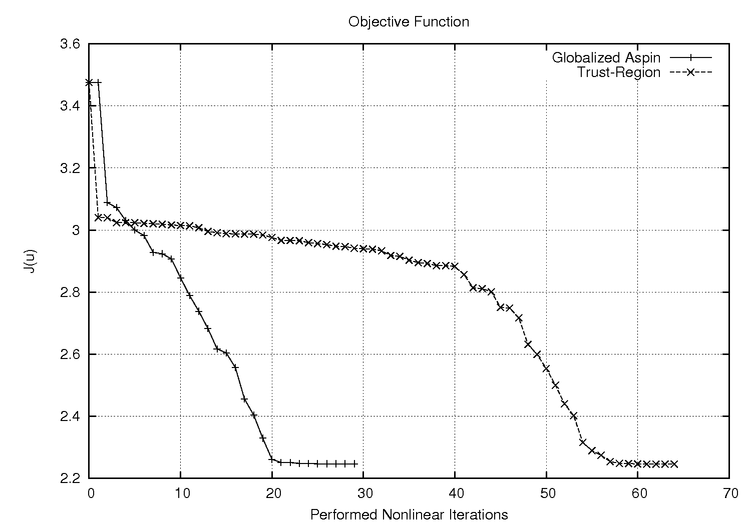
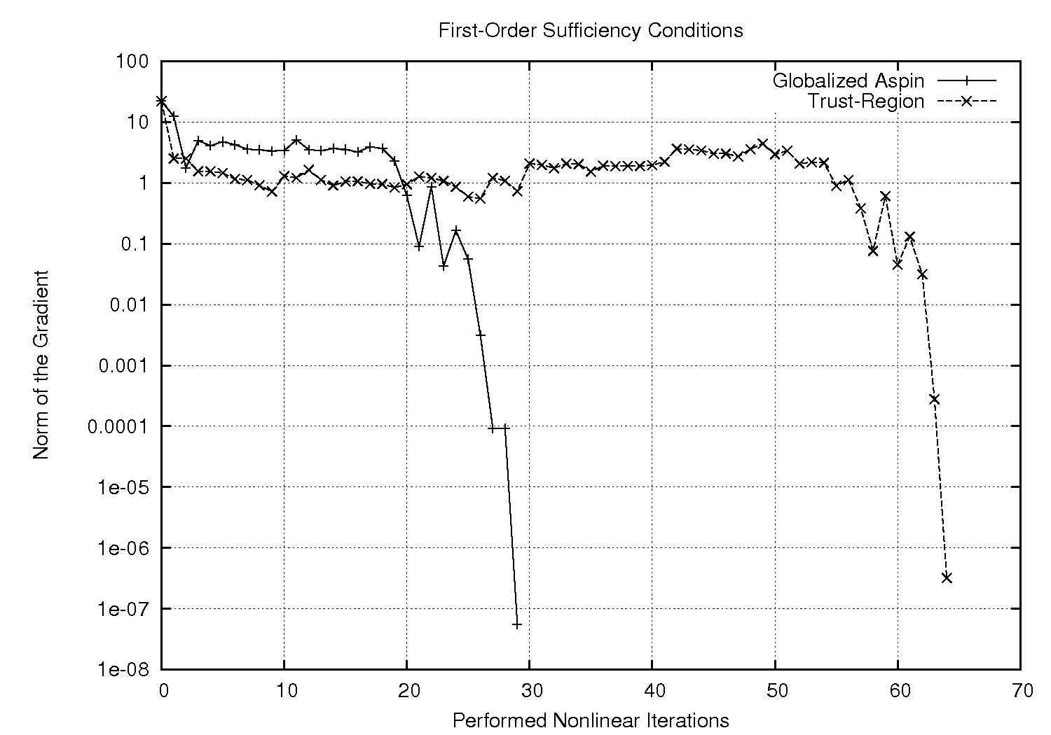
Computation on 240 Processors: Trust-Region vs. Globalized ASPIN

 
 
Computation on 1920 Processors: Trust-Region vs. Globalized ASPIN

 
 
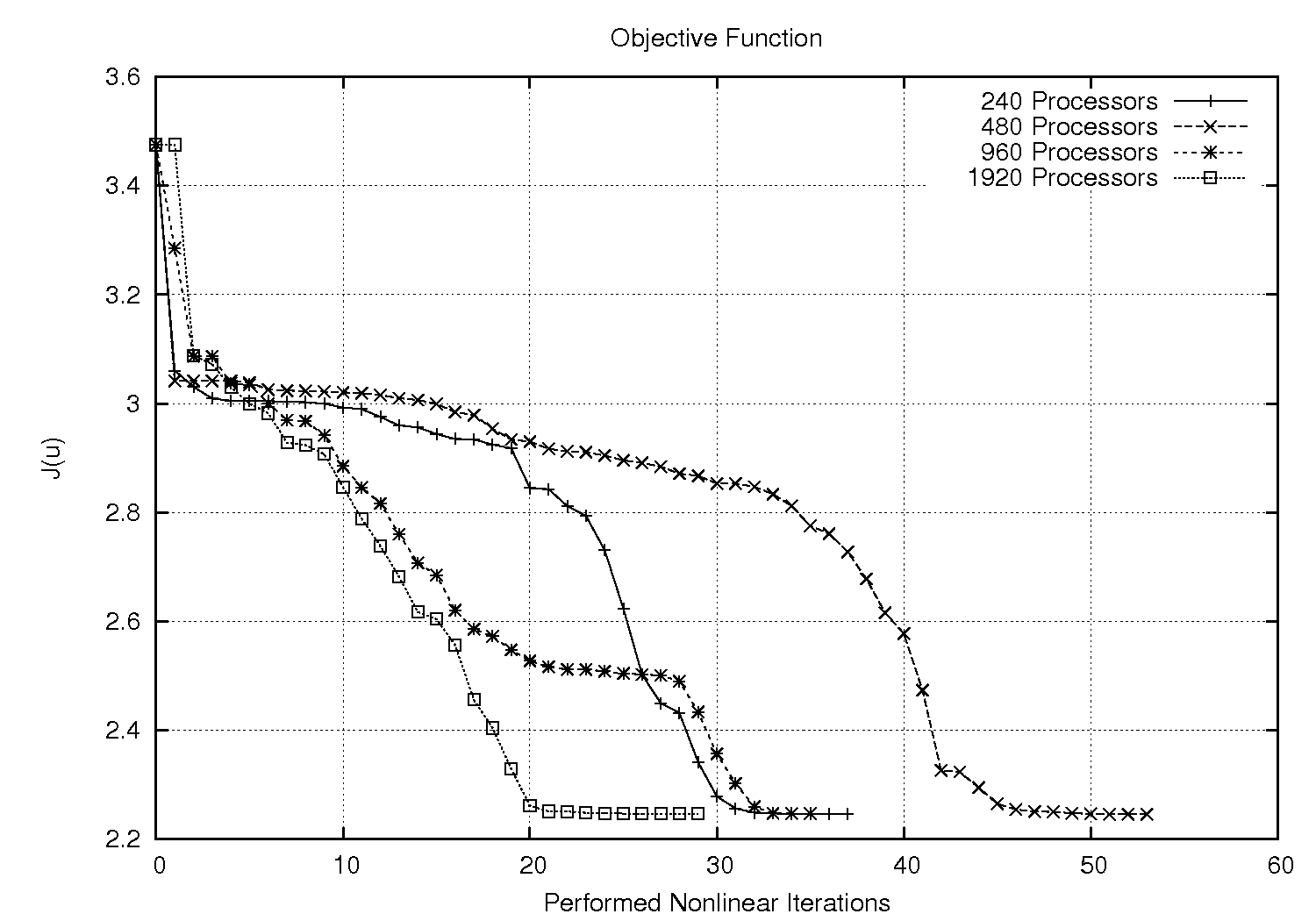
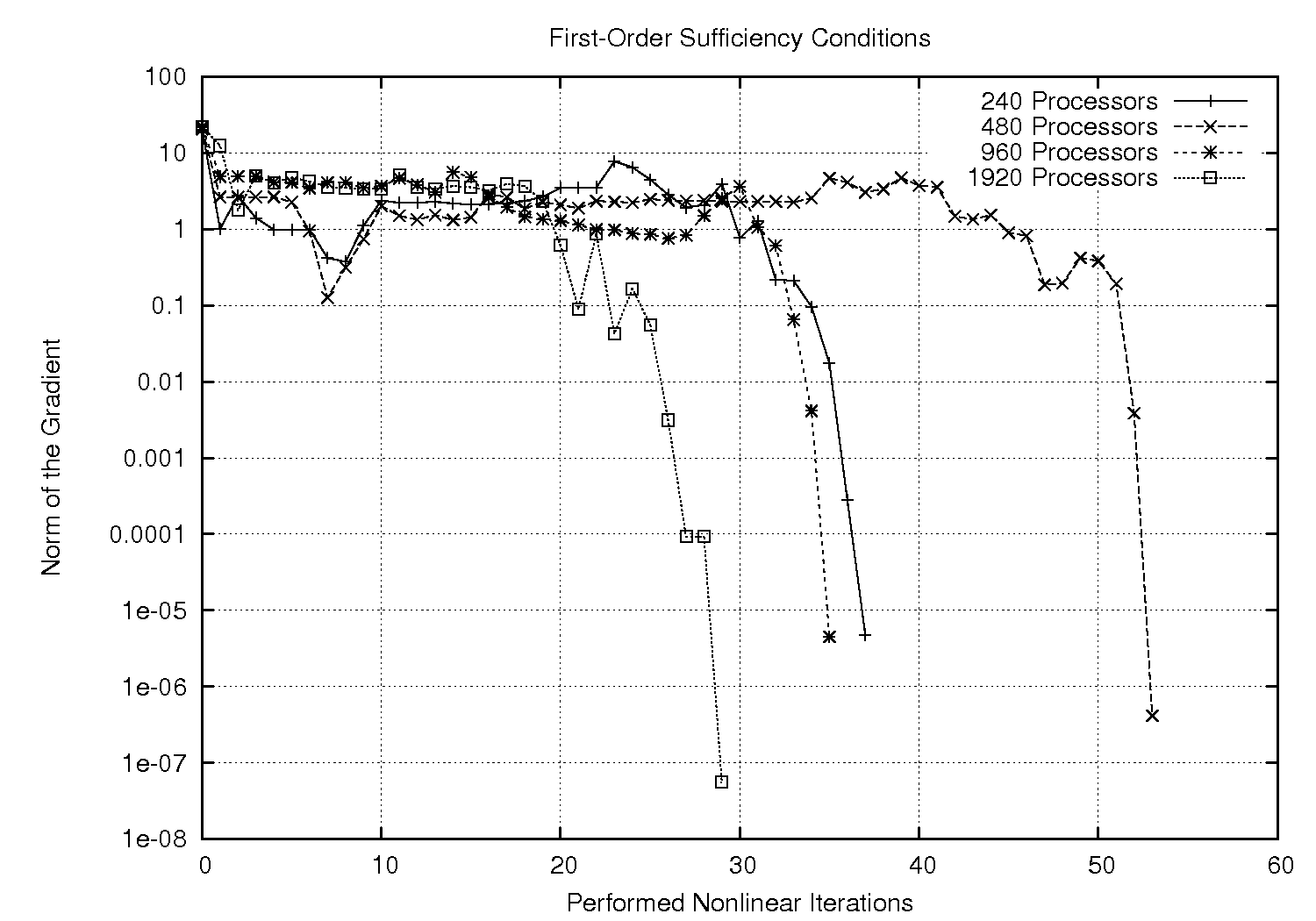
Comparison Globalized ASPIN with different Processor Numbers

Fig. 2: The first-order sufficiency conditions and the values of the objective function after each non-linear iteration for the solution of the example from Section 7.2 with 100,800 unknowns. Computation was carried out on $240$, $480$, $960$, $1920$ processors. Here, we compare a trust-region method with the globalized ASPIN approach, where both methods converge to exactly the same solution.

	Trust-Region	Globalized ASPIN
Overall Time	3293.95	2166.99
Linear Solver for global trust-region problem	3292.67	2042.96
Linear Solver in local solution phase	—	7.61
Assembling	12.71	68.09

Table 1: Computation times (in seconds) needed to solve Problem (1) on $240$ processors. Problem settings are described in Section 7.2.

	Trust-Region	Globalized ASPIN
Overall Time	2711.17	1238.76
Linear Solver for global trust-region problem	2722.98	1220.27
Linear Solver in local solution phase	—	0.66
Assembling	4.91	12.40

Table 2: Computation times (in seconds) needed to solve Problem (1) on $1920$ processors. Problem settings are described in Section 7.2.

	240 cores	480 cores	960 cores	1920 cores
Overall Time	2166.99	2044.14	1102.32	1238.76
Linear Solver global TR problem	2042.96	1918.69	1058.14	1220.27
Linear Solver local	7.61	6.65	1.77	0.66
Assembling	68.09	71.49	23.77	12.40
Nonlinear Iterations	37	53	35	29

Table 3: Computation times (in seconds) needed to solve Problem (1) with different numbers of processors. Problem settings are described in Section 7.2. The poor scaling from $960$ to $1920$ cores is due to the small local problem size. On the other hand, the poor scaling between $240$ and $480$ cores can be explained by an increased number of non-linear iterations.

7.1.2 Local Solution and Recombination

For the computation of $\tilde{g}_{i}$, we employ the linear recombination approach from Section 5.4.2. As we pointed out, it is therefore not important which method we use for the local computations on the subsets. In our implementation, we employ a trust-region approach. This trust-region method either stops the local computation if the norm of the local gradient is lower than $10^{-9}$ or after 20 trust-region iterations.

7.1.3 Nonlinear Solution Process

The numerical results of the following sections compare the runtime and convergence of the presented globalized ASPIN strategy to a trust-region strategy without the preconditioning step. Both globalization strategies employ a parallelized Steihaug Toint conjugate gradient method [23, 24] for the solution of the arising trust-region subproblems, which employs a multigrid method as a smoother. In order to be able to prove a sufficient decrease, we only accept the computed trust-region steps, if their predicted reduction is better than the one of the respective Cauchy step.

Alternatively, one might employ a Lanczos method (for broad survey see [9]) for the solution of the arising quadratic programming problems.

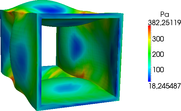
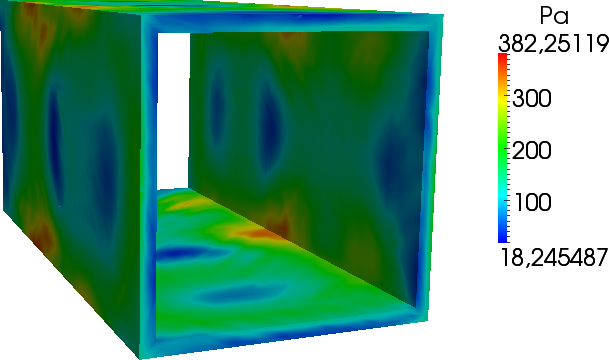
7.2 Deformation of a Hollow Brick

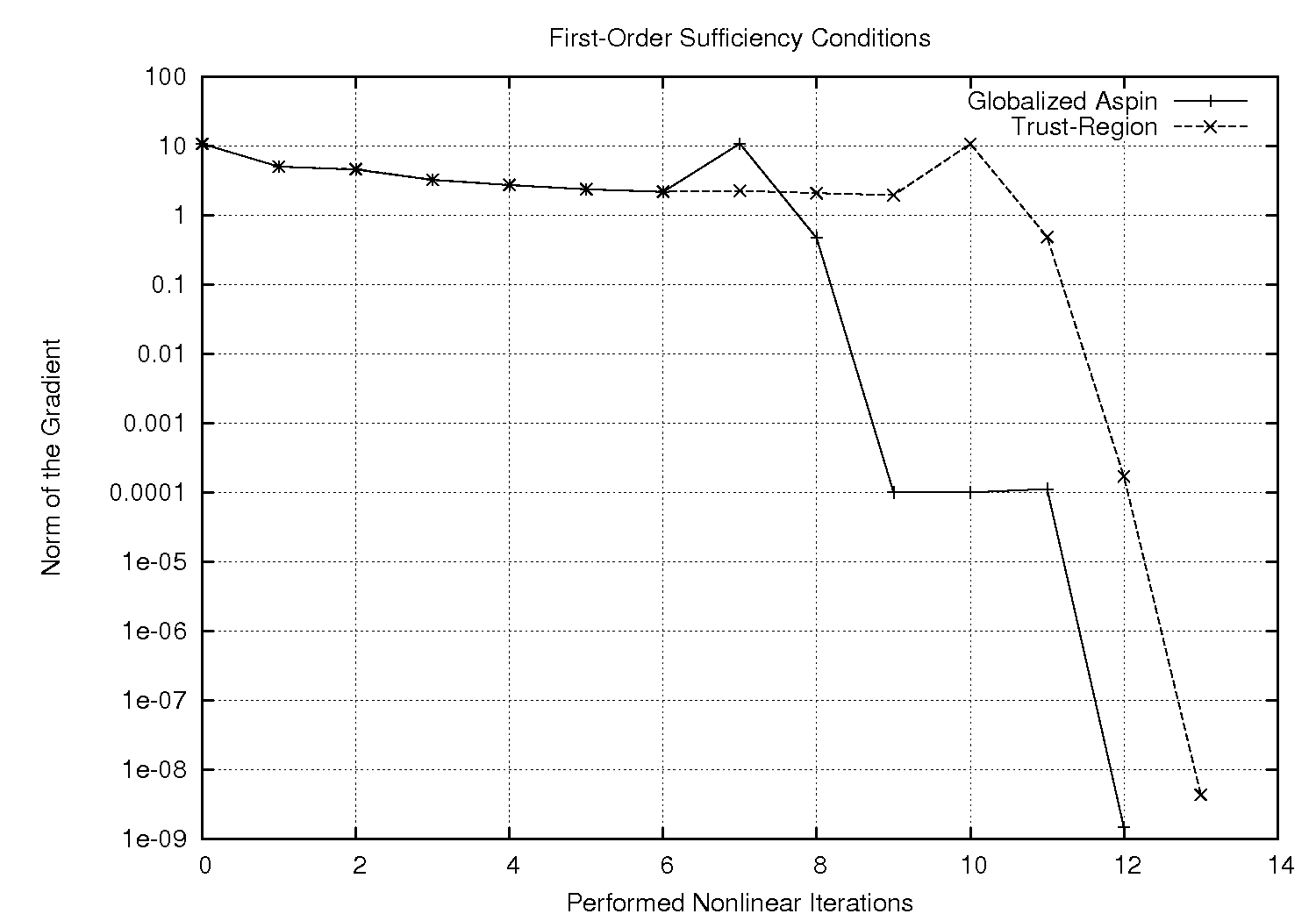
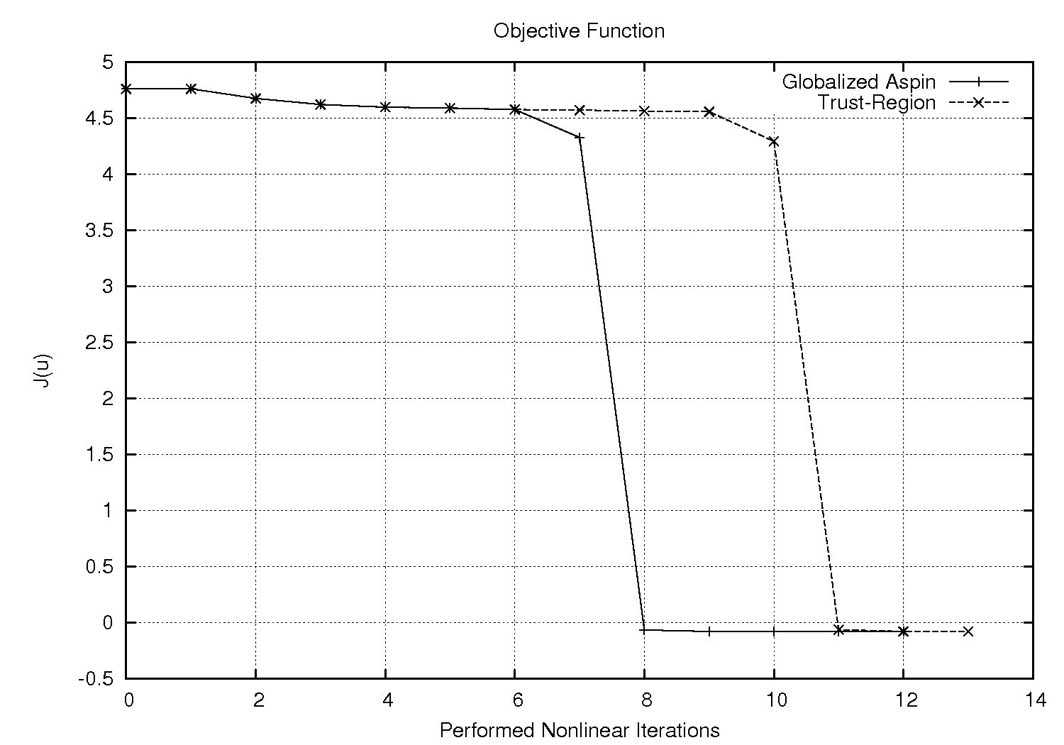
In this section, we present computational results showing the efficiency of the new approach for non-linear programming problems in non-linear elasticity. As a reference application, we consider the compression of a brick as shown in Figure 1. The brick itself is a hollow geometry with dimension $(1.0,1.0,2.0)$ and is compressed by $10.0\%$. The chosen material parameters are $E=3000$Pa and $\nu=0.3$.

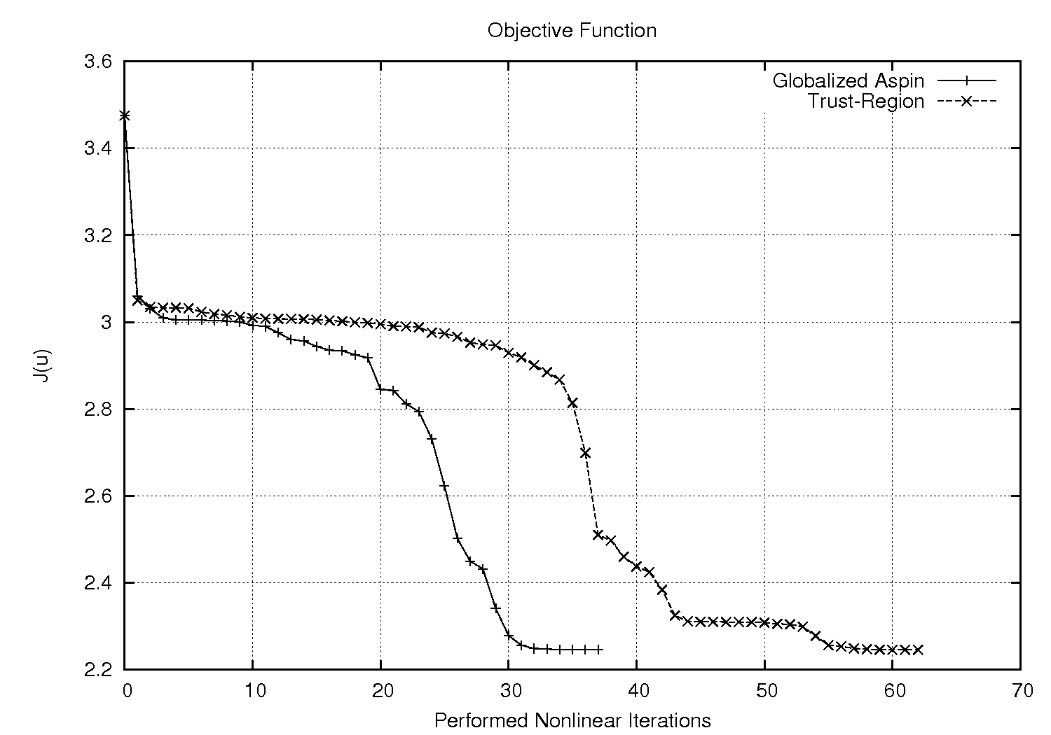
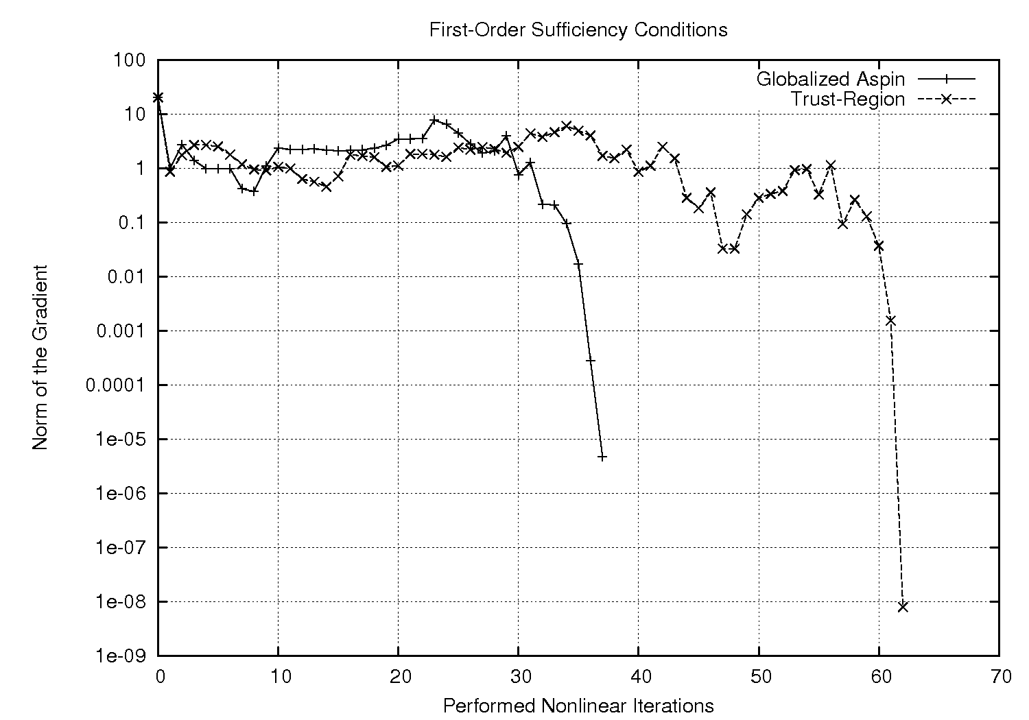
The solution of the resulting minimization problem is shown in Figure 1, the values of the objective function and the gradients are given in Figure 2. Moreover, computation times of the respective strategies are given in Tables 1, 2 and 3.

Note that in Figure 2, the number of non-linear iterations needed to reach a specific reduction in the objective function $J$ sometimes decreases substantially, when the number of processors is increased. This would not be the expected behavior usual for parallel Schwarz methods for linear problems. However, we here are not dealing with a parallelization of the Newton method, but our method is a non-linear, parallel solver, whose behavior changes, when we employ a different domain decomposition, as different and more quadratic models are employed.

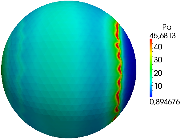
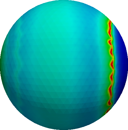
7.3 Deformation of a Hollow Sphere

As second application, we consider the very slight compression of a sphere, as shown in Figure 3. The sphere is a hollow geometry with inner radius $0.4$ and outer radius $0.5$. The chosen material parameters are $E=3000$Pa and $\nu=0.3$. In this second example, the sphere is fixed at one side, i.e., we apply $0$ displacements at the Dirichlet boundary. On the opposite side of the geometry, we apply constant forces, i.e., $(40,\ldots,40)^{T}$ as Neumann values.

Fig. 3: Numerical result of the example from Section 7.2 with 828,864 unknowns, where the initial geometry is deformed according to the solution of Equation (1) (left figure). Right figure: the initial geometry, which is – beside the stresses – only slightly different from the deformed configuration.

Computation on 32 cores
 
Computation on 64 cores

Fig. 4: The first-order sufficiency conditions and the values of the objective function after each non-linear iteration for the solution of the example from Section 7.2 with 828,864 unknowns. Computation was carried out on 32 and 64 processors. Here, we compare a trust-region method with the globalized ASPIN approach, where both methods converge to exactly the same solution.

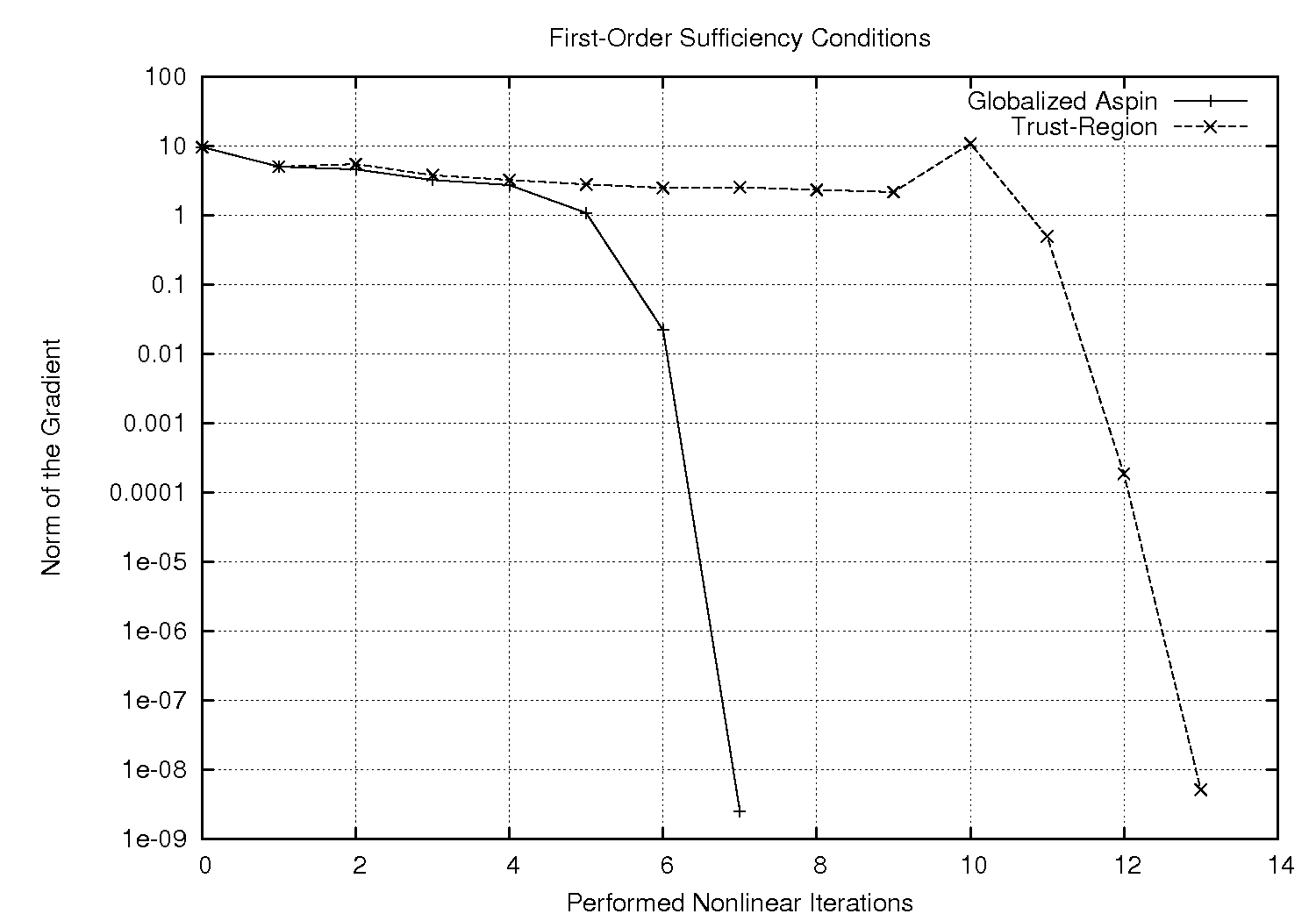
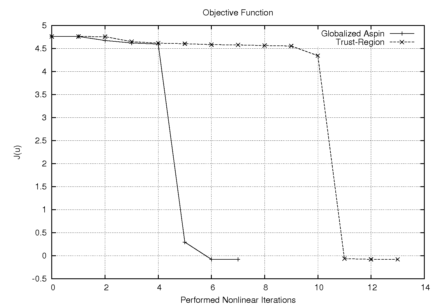
The solution of the resulting minimization problem is shown in Figure 3, the values of the objective function and the gradients are given in Figure 4. Moreover, computation times of the respective strategies are given in Table 4. Note that also in this case, all computations end in the same minimum.

Computation on 32 cores
Trust-Region Globalized ASPIN Overall Time 3323.96 2576.61 Linear Solver for global trust-region problem 3211.49 1796.65 Linear Solver in local solution phase — 442.23 Assembling 70.39 299.05  
 
 
Computation on 64 cores
Trust-Region Globalized ASPIN Overall Time 1805.94 2211.23 Linear Solver for global trust-region problem 1748.03 1653.55 Linear Solver in local solution phase — 224.55 Assembling 38.80 204.65 .

Table 4: Computation times (in seconds) needed to solve problem Equation (1) on 64 processors. Problem settings are described in Section 7.3

8 Conclusions

In this article, we presented and analyzed a globalization strategy which extends the ASPIN method presented in [3]. The key idea of this globalization approach is to consider ASPIN’s non-linearly preconditioned Newton step as the first-order conditions of a particular quadratic programming problem, which we refer to as preconditioned quadratic model.

Due to the interpretation of this preconditioned model as a perturbed model, one can enforce convergence of the method by employing a trust-region algorithm on the one hand and by controlling the perturbation, on the other. Approaches for controlling perturbations were introduced for instance in [25, 22, 8, 10], where the focus is on numerical differentiation and the solution of constrained non-linear programming problems. Here, however, the perturbation results from the fact that the gradient is based on the sum of local correction vectors for related, local non-linear programming problems. A particular feature of the current algorithm is that it exploits (massive) parallelism by solving these local non-linear programming problems asynchronously and in parallel. In this context, we introduced another trust-region radius, whose purpose is to control the perturbation of the preconditioned gradient. We introduced two strategies to compute the preconditioned gradients, which satisfy this perturbation constraint. Furthermore, our numerical results reveal the stability of the novel method and, in comparison to the trust-region method, a significant speed-up.

References

- [1] J. Arnal, V. Migallòn, J. Penadès, and D. B. Szyld. Newton additive and multiplicative Schwarz iterative methods. IMA Journal of Numerical Analysis, 28(3):143–161, 2008.
- [2] P. Bastian, K. Birken, K. Johannsen, S.Lang, N. Neuß, H. Rentz-Reichert, and C.Wieners. UG – a flexible software toolbox for solving partial differential equations. Computing and Visualization in Science, 1:27–40, 1997.
- [3] X-C. Cai and D. E. Keyes. Nonlinearly preconditioned inexact Newton algorithms. SIAM J. Sci. Comput., 24(1):183–200, 2002.
- [4] X.-C. Cai, D. E. Keyes, and L. Marcinkowski. Nonlinear additive Schwarz preconditioners and application in computational fluid dynamics. Int. J. Numer. Methods Fluids, 40(12):1463–1470, 2002.
- [5] X.-C. Cai, D. E. Keyes, and D. Young. A nonlinear additive Schwarz preconditioned inexact Newton method for shocked duct flows. Debit, N. (ed.) et al., Domain decomposition methods in science and engineering. Papers of the thirteenth international conference on domain decomposition methods, Lyon, France, October 9–12, 2000. Barcelona: International Center for Numerical Methods in Engineering (CIMNE). Theory Eng. Appl. Comput. Methods, 345-352 (2002)., 2002.
- [6] P. G. Ciarlet. Mathematical elasticity, volume I: Three-dimensional elasticity. Studies in Mathematics and its Applications, 20(186):715–716, 1988.
- [7] T. F. Coleman and Y. Li. An interior trust region approach for nonlinear minimization subject to bounds. SIAM J. Optim., 6:418–445, May 1996.
- [8] A. R. Conn, N. Gould, A. Sartenaer, and Ph. L. Toint. Global convergence of a class of trust region algorithms for optimization using inexact projections on convex constraints. SIAM Journal on Optimization, 3(1):164–221, 1993.
- [9] A. R. Conn, N. I. M. Gould, and Ph. L. Toint. Trust-region methods. Society for Industrial and Applied Mathematics, Philadelphia, PA, USA, 2000.
- [10] U. Felgenhauer. Algorithmic stability analysis for certain trust region methods. Number 195 in Lecture Notes in Pure and Applied Mathematics. Marcel Dekker, New York, Basel, 1997.
- [11] M. C. Ferris and O. L. Mangasarian. Parallel variable distribution. SIAM J. Optim., 4(4):815–832, 1994.
- [12] S. Gratton, A. Sartenaer, and P. L. Toint. Recursive trust-region methods for multiscale nonlinear optimization. SIAM Journal on Optimization, 19(1):414–444, 2008.
- [13] C. Groß. A Unifying Theory for Nonlinear Additively and Multiplicatively Preconditioned Globalization Strategies Convergence Results and Examples From the Field of Nonlinear Elastostatics and Elastodynamics. PhD thesis, Bonn International Graduate School, University of Bonn, 07 2009. Online-Publikationen an deutschen Hochschulen, Bonn, Univ., Diss., 2009, URN: urn:nbn:de:hbz:5N-18682.
- [14] C. Groß and R. Krause. Import of geometries and extended informations into obslib++ using the exodus ii and exodus parameter file formats. Technical Report 712, Institute for Numerical Simulation, University of Bonn, Germany, January 2008.
- [15] C. Groß and R. Krause. A new class of non–linear additively preconditioned trust–region strategies: Convergence results and applications to non-linear mechanics. INS preprint 904, Institute for Numerical Simulation, University of Bonn, 03 2009.
- [16] C. Groß and R. Krause. On the convergence of recursive trust–region methods for multiscale non-linear optimization and applications to non-linear mechanics. SIAM J. Numer. Anal., 47(4):3044–3069, 09 2009.
- [17] R. Krause. Obslib++, an object oriented toolbox for constrained minimization problems. Technical report, Institute for Numerical Simulation, University of Bonn, 2006.
- [18] R. Krause, A. Rigazzi, and J. Steiner. A parallel multigrid method for constrained minimization problems and its application to friction, contact, and obstacle problems. Computing and Visualization in Science, 2015. to appear.
- [19] O.L. Mangasarian. Parallel gradient distribution in unconstrained optimization. SIAM J. Control Optimization, 33(6):1916–1925, 1995.
- [20] Stephen G. Nash. A multigrid approach to discretized optimization problems. Optimization Methods and Software, 14(1-2):99–116, 2000.
- [21] J. Nocedal and S. Wright. Numerical Optimization. Springer Series in Operations Research and Financial Engineering. Springer, 2nd edition, 2006.
- [22] R.G.Carter. Numerical experience with a class of algorithms for nonlinear optimization using inexact function and gradient information. SIAM Journal on Scientific and Statistical Computing, 14(2):368–388, 1993.
- [23] Trond Steihaug. The conjugate gradient method and trust regions in large scale optimization. SIAM Journal on Numerical Analysis, 20(3):626–637, 1983.
- [24] Ph. L. Toint. Towards an efficient sparsity exploiting Newton method for minimization. Sparse matrices and their uses, page 1981, 1981.
- [25] Ph. L. Toint. Global convergence of a class of trust-region methods for nonconvex minimization in Hilbert space. IMA J. Numer. Anal., 8(2):231–252, 1988.
- [26] M. Ulbrich, S. Ulbrich, and M. Heinkenschloss. Global convergence of trust-region interior-point algorithms for infinite-dimensional nonconvex minimization subject to pointwise bounds. SIAM Journal on Control and Optimization, 37(3):731–764, 1999.